ANL-HEP-PR-04-88 CERN-TH/2004-208 CU-TP-1119 EFI-04-32 FERMILAB-PUB-04/226-T Warped Fermions and Precision Tests

Abstract

We analyze the behavior of Standard Model matter propagating in a slice of AdS₅ in the presence of infrared-brane kinetic terms. Brane kinetic terms are naturally generated through radiative corrections and can also be present at tree level. The effect of the brane kinetic terms is to expell the heavy KK modes from the infrared-brane, and hence to reduce their coupling to the localized Higgs field. In a previous work we showed that sizable gauge kinetic terms can allow KK mode masses as low as a few TeV, compatible with present precision measurements. We study here the effect of fermion brane kinetic terms and show that they ameliorate the behavior of the theory for third generation fermions localized away from the infrared brane, reduce the contribution of the third generation quarks to the oblique correction parameters and mantain a good fit to the precision electroweak data for values of the KK masses of the order of the weak scale.

1 Introduction

The hierarchy between the apparent Planck scale and electroweak scale is very mysterious, and leads us to believe that the Standard Model (SM) is most likely only an effective theory which breaks down at the electroweak scale. This belief in fact drives much of the present activity in particle physics, both to propose alternatives for physics beyond the SM and to explore their consequences. One of the more intriguing possibilities is the Randall-Sundrum (RS) model [1]. This model invokes a warped metric (of curvature $k$) to explain how the two scales can coexist quite naturally: the Planck scale $M_{P}$ is the fundamental scale of the bulk as a whole, and is the apparent scale for gravity as a result of the graviton wave function having most of its support at the point where the warp factor is largest. The Higgs potential, however, is naturally at the weak scale as a result of it living on the other side of the extra dimension where the warp factor renders the natural scale of order $M_{P}e^{-kL}\sim 1$ TeV. This fixes the size of the extra dimension such that $kL\sim 30$.

The RS hierarchy solution requires only that the Higgs be confined to the IR boundary at $y=L$ ($y$ is the coordinate in the compact dimension). It does not require that the rest of the SM fields be with the Higgs on the IR boundary. A particularly attractive extension has gauge fields and fermions in the bulk [2]-[5], allowing one to address grand unification, absence of TeV-scale FCNC effects, and perhaps even the observed flavor structure for the SM fermions itself. The AdS/CFT connection allows such theories an alternate interpretation as a nearly conformal 4d theory, with conformal breaking at the TeV scale [6].

Having promoted the SM gauge fields and fermions to extra-dimensional fields, the possibility arises that there will be brane interactions which mimic their 5d kinetic terms [7]-[10]. These terms appear as irrelevant operators in the 5d theory, but as all interactions are already irrelevant, they should be considered a generic feature of any effective theory for extra dimensions. A specific UV completion could in principle predict their size, but in the absence of one, they are part of the most general extra-dimensional model which one may consider. Further, as is usually the case with any term not forbidden by a symmetry, they will be generated radiatively even if the underlying physics renders them small at tree level. These terms are of particular importance on the IR brane of a warped theory, where the warping enhances their impact, and it is therefore important to study their physical effects.

The theory with gauge fields in the bulk can potentially feel strong bounds from precision electroweak (EW) data [11]-[17]. The issue is that the localized Higgs VEV can induce substantial mixing between the ordinary $W$ and $Z$ bosons with their KK brethren, distorting their properties at a level in disagreement with precision data. In the most simple theories, bounds on the order of 20 TeV can be derived, rendering the theory impossible to discover at future colliders and re-introducing fine-tuning in the Higgs potential at a level of $10^{-3}$.

Some of these constraints may be ameliorated by including brane kinetic terms for the gauge bosons [16] or by imposing a custodial $SU(2)$ symmetry [18]. Still others could be improved by moving the fermions away from the IR brane. However, one quickly runs into a problem with this second solution: the large top mass indicates that the top is strongly coupled to the Higgs, and in fact the Kaluza-Klein (KK) modes are even more strongly coupled than the zero mode. If the top lies far from the IR brane, the KK modes become so strongly coupled that the theory quickly loses a perturbative description. Thus, there is a kind of “tug of war” between the requirements of small EW corrections and a perturbative top Yukawa interaction.

A separate issue related to the geometrical picture of fermion flavor arises from non-universal couplings which distinguish the bottom quark. The small masses of the first and second generation fermions motivate their being located close to the Planck brane, whereas the large top mass requires that the top-quark (including left-handed top, and thus also left-handed bottom) be located close to the TeV brane. This leads to a non-oblique correction to the $Z$-$b_{L}$-$\overline{b}_{L}$ vertex which ruins the observed agreement of the predicted $R_{b}$ with its measured value and can induce flavor-changing neutral currents at an unacceptable level.

In this article we explore a new class of brane kinetic terms, those relevant for the fermion fields. As argued above, they are present in any self-consistent description of the extra dimension anyway, and they further have great potential to relax some of the EW precision bounds. In particular, since they expell the KK modes of the fermions from the IR brane, they allow for a wider region of localized top quarks without the strong coupling problems alluded to above. This in itself allows one to consider regions of parameters where the couplings of the SM fermions to the gauge KK modes are strongly suppressed or may altogether vanish. As a result, contributions to the $S$ parameter and possible additional four fermion interactions can be made small, which can lead to a much more comfortable situation from the perspective of the EW fit. They also suppress some contributions to the $T$ parameter from KK modes of top, and thus are directly helpful in their own right. There are still potentially large contributions to the $T$ parameter coming from the nonuniversal modification of the $W$ and $Z$ gauge boson wavefunctions, that arises from the mixing with their KK modes through the localized Higgs. As mentioned above, these effects can be suppressed either by including brane kinetic terms for the gauge fields, or by imposing a custodial symmetry. The net result is that in the presence of fermion brane kinetic terms the EW fit allows lower KK mode masses than in a theory without the fermion brane kinetic terms, and thus more opportunity to observe KK modes at future colliders and less EW fine-tuning in the Higgs potential.

This article is organized as follows. In Section 2 we introduce brane kinetic terms for the even components of bulk fermions, and derive the spectrum and wave functions. In Section 3 we examine the role such terms play in strong coupling limits for fields coupled to the IR brane. We find that even for moderate values of the infrared brane kinetic term coefficient, the constraint from the top quark mass on the fifth dimensional Yukawa coupling is significantly relaxed. In Section 4 we examine the implications for the EW fit. Finally, in Section 5 we conclude.

2 5D Lagrangian and KK Decomposition

We begin by setting up notation, and deriving the KK decomposition for a bulk fermion, including brane kinetic terms. The background metric can be written as

$$ds^{2}=G_{MN}dx^{M}dx^{N}=e^{-2\sigma}\eta_{\mu\nu}dx^{\mu}dx^{\nu}+dy^{2}~{},$$ (1)

with $\eta_{\mu\nu}=\mbox{diag}(-1,+1,+1,+1)$, $\sigma(y)=k|y|$ and $0\leq y\leq L$. We use upper case roman letters for the 5d Lorentz indices, and lower case greek letters for the 4d ones. The Higgs field is localized on the $y=L$ brane (IR brane) where the fundamental scale is red-shifted to TeV values, thus solving the hierarchy problem. We assume that both the standard model gauge bosons and fermions live in the bulk, together with gravity.

The lagrangian for a freely gravitating fermion, including brane localized kinetic terms, can be written as

$$S=-\int d^{4}x\,\int_{0}^{L}dy\,\sqrt{-G}\,\{i\bar{\Psi}\Gamma^{A}e_{A}^{M}D_{M}\Psi+iM(y)\bar{\Psi}\Psi+2\alpha_{f}\delta(y-L)i\bar{\Psi}_{L}\gamma^{a}e_{a}^{\mu}\partial_{\mu}\Psi_{L}\}~{}.$$ (2)

We use ($\Gamma$, $\gamma$) for (5d,4d) $\gamma$-matrices and ($A$, $a$) for the (5d,4d) tangent-space Lorentz indices. $G$ represents the determinant of the (5d) metric, $e$ is the vielbein, $D_{M}$ is the covariant derivative, including the spin connection, and $\alpha_{f}$ is the coefficient of the brane localized kinetic term. Note that $\alpha_{f}$ has dimension of ${\rm mass}^{-1}$. The $\delta$-function is normalized so that $\int_{0}^{L}2\delta(y)dy=1$.

The boundary conditions at $y=0,L$ are chosen so that the low-energy theory is chiral [3]. For definiteness, in the above case only the left-handed component $\Psi_{L}$ has a zero mode. The mass function is $M(y)=c_{f}\sigma^{\prime}$ (i.e., it is an odd mass term), where the dimensionless bulk mass parameter $c_{f}$ essentially determines the localization of the massless (zero) mode.

The above action is not the most general one at the quadratic level. We are only including brane terms on the IR brane, and then only so for the even chirality and involving $\partial_{\mu}$ as opposed to $\partial_{5}$. The first choice is purely for phenomenological purposes, since the UV brane kinetic terms are irrelevant for the KK mode spectrum. One way to understand this is that the wave function of KK modes whose masses are $\sim O({\rm TeV})$ are localized near the IR brane and are therefore relatively insensitive to the UV brane terms. We will briefly consider the effect of UV brane terms on the EW fit in Sec. 4.2 below.

The second choice, adding kinetic terms only for the even field components, can be thought of as a prescription for some of the UV physics. In the absence of localized kinetic terms, the even fields ($\Psi_{L}$) will couple to the brane whereas the odd fields ($\Psi_{R}$) will not (the odd wave functions vanish on the brane as a result of the odd boundary conditions), and therefore operators like $i\bar{\Psi}_{R}\gamma^{a}e_{a}^{\mu}\partial_{\mu}\Psi_{R}$ vanish on the brane. Furthermore, if this term is absent, it will not be perturbatively generated, and thus this situation is technically natural.

One may still consider the nonvanishing operator $i(\bar{\Psi}_{L}\partial_{5}\Psi_{R}+\partial_{5}\bar{\Psi}_{R}\Psi_{L})$ localized on the brane, although its interpretation requires a careful regularization of the brane thickness. From a practical point of view, the choice of Eq. (2) is convenient because it insures that the $\Psi_{L}$ wave functions are continuous on the brane, and thus their couplings to brane fields are well-defined in the infinitely narrow brane approximation.

2.1 KK Decomposition

We expand the fermion field in KK modes as

$$\Psi_{L,R}(x,y)=e^{3\sigma/2}\sum_{n}\psi^{n}_{L,R}(x)f_{L,R}^{n}(y)~{},$$ (9)

where the KK mode wavefunctions, $f^{n}_{L,R}$, satisfy the set of coupled equations

$$\left[\partial_{5}+(c_{f}-1/2)\sigma^{\prime}\right]f_{L}^{n} = e^{\sigma}m_{n}f_{R}^{n}~{},$$ (10)

$$\left[-\partial_{5}+(c_{f}+1/2)\sigma^{\prime}\right]f_{R}^{n} = e^{\sigma}m_{n}f_{L}^{n}\left[1+2\alpha_{f}\delta(y-L)\right]~{},$$ (11)

and $m_{n}$ are the KK masses. In order to have canonically normalized kinetic terms in the 4d KK description, we choose the wavefunctions $f_{L,R}$ to satisfy the following orthonormality relations

$$\int_{0}^{L}dy\left[1+2\alpha_{f}\delta(y-L)\right]f^{n}_{L}f^{m}_{L} = \delta_{mn}$$

$$\int_{0}^{L}dyf^{n}_{R}f^{m}_{R} = \delta_{mn}~{}.$$ (12)

The appropriately normalized zero-mode wavefunction is

$$f_{L}^{0}(y) = \sqrt{\frac{k(1-2c_{f})}{e^{(1-2c_{f})kL}\left[1+(1-2c_{f})\alpha_{f}k\right]-1}}e^{(1/2-c_{f})\sigma}~{},$$ (13)

and the odd tower, by construction, does not contain a zero-mode. To solve for the massive KK mode wavefunctions we use Eq. (10) to find $f_{R}^{n}$,

$$f_{R}^{n}=\frac{e^{-\sigma}}{m_{n}}\left[\partial_{5}+(c_{f}-1/2)\sigma^{\prime}\right]f_{L}^{n}~{},$$ (14)

and replacing in Eq. (11) we have a second order differential equation for $f_{L}^{n}$:

$$\left[-\partial_{5}^{2}+2\sigma^{\prime}\partial_{5}-\left(1-\left(c_{f}+1/2\right)^{2}\right)(\sigma^{\prime})^{2}-(c_{f}-1/2)\sigma{{}^{\prime\prime}}\right]f_{L}^{n}=e^{2\sigma}m_{n}^{2}\left[1+2\alpha_{f}\delta(y-L)\right]f_{L}^{n}~{}.$$ (15)

Using $\sigma^{\prime\prime}=2k\left[\delta(y)-\delta(y-L)\right]$, we see that we have the boundary conditions

$$\left.\rule{0.0pt}{14.22636pt}\partial_{5}f_{L}^{n}\right|_{y=0} = \left.\left(\frac{1}{2}-c_{f}\right)kf_{L}^{n}\right|_{y=0}~{},$$ (16)

$$\left.\rule{0.0pt}{14.22636pt}\partial_{5}f_{L}^{n}\right|_{y=L} = \left[\left(\frac{1}{2}-c_{f}\right)k+\left.\rule{0.0pt}{14.22636pt}\alpha_{f}m_{n}^{2}e^{2kL}\right]f_{L}^{n}\right|_{y=L}~{}.$$ (17)

The solution to Eq. (15) in the bulk is

$$f^{n}_{L}(y)=A_{n}e^{\sigma}\left[J_{|c_{f}+1/2|}\left(\frac{m_{n}}{k}e^{\sigma}\right)+b_{n}J_{-|c_{f}+1/2|}\left(\frac{m_{n}}{k}e^{\sigma}\right)\right]~{},$$ (18)

where $A_{n}$ is fixed by the normalization condition Eq. (12), while the boundary conditions, Eqs. (16) and (17), determine $b_{n}$ and the KK spectrum by

$$b_{n} = -\frac{(c_{f}+1/2)J_{|c_{f}+1/2|}\left(\frac{m_{n}}{k}\right)+\frac{m_{n}}{k}J^{\prime}_{|c_{f}+1/2|}\left(\frac{m_{n}}{k}\right)}{(c_{f}+1/2)J_{-|c_{f}+1/2|}\left(\frac{m_{n}}{k}\right)+\frac{m_{n}}{k}J^{\prime}_{-|c_{f}+1/2|}\left(\frac{m_{n}}{k}\right)}$$ (19)

$$= -\frac{(c_{f}+1/2-\tilde{\alpha}_{f}\frac{m_{n}^{2}}{\tilde{k}})J_{|c_{f}+1/2|}\left(\frac{m_{n}}{\tilde{k}}\right)+\frac{m_{n}}{\tilde{k}}J^{\prime}_{|c_{f}+1/2|}\left(\frac{m_{n}}{\tilde{k}}\right)}{(c_{f}+1/2-\tilde{\alpha}_{f}\frac{m_{n}^{2}}{\tilde{k}})J_{-|c_{f}+1/2|}\left(\frac{m_{n}}{\tilde{k}}\right)+\frac{m_{n}}{\tilde{k}}J^{\prime}_{-|c_{f}+1/2|}\left(\frac{m_{n}}{\tilde{k}}\right)}~{},$$

where we defined $\tilde{k}=ke^{-kL}\sim O({\rm TeV})$ and $\tilde{\alpha}_{f}=\alpha_{f}e^{kL}\sim O({\rm TeV}^{-1})$. Note that like any other IR brane term, the localized fermion kinetic term is warped, and as a term with inverse mass dimension, the warping increases its importance at low energies. As usual, the consistency of the boundary conditions is what determines the mass eigenvalues $m_{n}$.

We can obtain approximate expressions for the wavefunctions of the lowest lying KK modes ($m_{n}\ll k$). When $c_{f}>\frac{1}{2}(1+1/kL)$, the eigenvalue equation reduces to $b_{n}={\cal{O}}(m_{n}/k)^{2c_{f}-1}\ll 1$, i.e.

$$J_{c_{f}-1/2}(x_{n})\approx\alpha_{f}kx_{n}J_{c_{f}+1/2}(x_{n})~{},$$ (20)

where $m_{n}\equiv x_{n}\tilde{k}$, and the wavefunctions become

$$f^{n}_{L}(y) \approx A_{n}e^{ky}J_{c_{f}+1/2}(x_{n}e^{-k(L-y)})~{},$$

$$A_{n} = \frac{e^{-kL}}{J_{c_{f}+1/2}(x_{n})}\sqrt{\frac{2k}{1+(1-2c_{f})\alpha_{f}k+\alpha_{f}^{2}k^{2}x_{n}^{2}}}~{}.$$ (21)

In this case, when the localized kinetic term is large, $\alpha_{f}k\gg 1$, one of the modes becomes light with $m\simeq\sqrt{(2c_{f}+1)/(\alpha_{f}k)}\,\tilde{k}$.

When $c_{f}<\frac{1}{2}(1-1/kL)$, the eigenvalue equation reduces to

$$J_{1/2-c_{f}}(x_{n})\approx-\alpha_{f}kx_{n}J_{-c_{f}-1/2}(x_{n})~{},$$ (22)

and the wavefunctions are now given by

$$f^{n}_{L}(y) \approx A_{n}e^{ky}J_{-c_{f}-1/2}(x_{n}e^{-k(L-y)})~{},$$

$$A_{n} = \frac{e^{-kL}}{J_{-c_{f}-1/2}(x_{n})}\sqrt{\frac{2k}{1+(1-2c_{f})\alpha_{f}k+\alpha_{f}^{2}k^{2}x_{n}^{2}}}~{}.$$ (23)

In this case there is no light mode.

For $c_{f}=1/2$, the wavefunctions read

$$f^{n}_{L}(y)=A_{n}e^{\sigma}\left[J_{1}\left(\frac{m_{n}}{k}e^{\sigma}\right)+b_{n}Y_{1}\left(\frac{m_{n}}{k}e^{\sigma}\right)\right]~{},$$ (24)

and the eigenvalues are now given by

$$b_{n} = -\frac{J_{0}\left(\frac{m_{n}}{k}\right)}{Y_{0}\left(\frac{m_{n}}{k}\right)}$$ (25)

$$= -\frac{J_{0}\left(\frac{m_{n}}{k}e^{kL}\right)-m_{n}\,\tilde{\alpha}_{f}J_{1}\left(\frac{m_{n}}{k}e^{kL}\right)}{Y_{0}\left(\frac{m_{n}}{k}e^{kL}\right)-m_{n}\,\tilde{\alpha}_{f}Y_{1}\left(\frac{m_{n}}{k}e^{kL}\right)}~{}.$$

The normalization factor, $A_{n}$, is not particularly simple and should be calculated from Eq. (12).

2.2 Mixed Position/Momentum Space Propagator

When computing loops or performing sums over all KK modes in the tower, the explicit decomposition is not the most convenient way to proceed. It is simpler to employ the propagator in mixed position/momentum space which implicitly includes the sum over all of the KK modes. Thus, in this section we compute the fermion propagator which shall be of use in Section 3 in estimating how strong a brane coupling involving the fermion can be made before the theory loses predictivity.

To be definite, we calculate the propagator by assuming that the boundary conditions are such that the zero mode is left-handed. The defining equation for the fermion propagator in the presence of a brane localized kinetic term for the left-handed components, as in Eq. (2), is then

$$i\left(\Gamma^{A}{e_{\!A}}^{\!M}D_{M}+M\right)G(X,X^{\prime})+2\delta(L-y)\alpha_{f}i\Gamma^{a}{e_{\!a}}^{\!\mu}P_{L}\partial_{\mu}G(X,X^{\prime})=\frac{i}{\sqrt{-G}}\delta^{(5)}(X-X^{\prime})~{},$$ (26)

where $M=c_{f}\sigma^{\prime}$ is the $Z_{2}$-odd bulk mass that determines the localization of the zero-mode, and $X=(x^{\mu},y)$. We Fourier transform Eq. (26) along the four noncompact coordinates and define the propagators for the various chiralities by $G_{LL}\equiv P_{L}GP_{R}=\langle\Psi_{L}\overline{\Psi_{L}}\rangle$, $G_{RL}\equiv P_{R}GP_{R}=\langle\Psi_{R}\overline{\Psi_{L}}\rangle$, etc., where $\Psi$ is a generic 5D fermion and $P_{L,R}$ are the left- and right-handed chirality projectors.

Since only the KK tower that contains a zero-mode couples to the brane, we concentrate on the propagator for the left handed components, $G_{LL}$. We may isolate it by first projecting onto Eq. (26) by $P_{L}$ from the left and by $P_{R}$ from the right to obtain

$$G_{RL}=-i\frac{e^{-\sigma}}{\not{\!p}}\left[\partial_{y}-(2-c_{f})\sigma^{\prime}\right]G_{LL}~{}.$$ (27)

Repeating the same projection after applying the operator $i\left(\Gamma^{A}{e_{\!A}}^{\!M}D_{M}-M\right)$ to Eq. (26) gives a second equation that relates $G_{LL}$ and $G_{RL}$, and using Eq. (27) to eliminate $G_{RL}$ we obtain a second order differential equation for $G_{LL}$:

$$\left\{\partial_{y}^{2}-\sigma^{\prime}\partial_{y}-c_{f}(c_{f}+1){\sigma^{\prime}}^{2}+c_{f}\sigma^{\prime\prime}-e^{2\sigma}p^{2}\left[1+2\delta(L-y)\alpha_{f}\right]\right\}G^{p}_{+}(y,y^{\prime})=-e^{3\sigma}\delta(y-y^{\prime})~{},$$ (28)

where we defined $G_{+}$ by $G_{LL}=iP_{L}\not{\!p}\,e^{2\sigma}G_{+}$, and the subscript “$+$” refers to our choice of $Z_{2}$-even boundary conditions for the left-handed spinor components. Note that due to the metric signature in Eq. (1), $p^{2}<0$ in the on-shell region and the solution to Eq. (26) can be directly interpreted as the Euclidean space propagator. The boundary conditions to be applied on $G_{+}$ are

$$\left.\rule{0.0pt}{11.38109pt}\partial_{5}G_{+}\right|_{y=0} = \left.\rule{0.0pt}{11.38109pt}-c_{f}kG_{+}\right|_{y=0}~{},$$

$$\left.\rule{0.0pt}{11.38109pt}\partial_{5}G_{+}\right|_{y=L} = \left.\rule{0.0pt}{11.38109pt}-c_{f}kG_{+}\right|_{y=L}-\left.\rule{0.0pt}{11.38109pt}\alpha_{f}p^{2}e^{2kL}G_{+}\right|_{y=L}~{},$$ (29)

and the explicit solution is

$$e^{2\sigma(y)}G_{+}^{p}(y,y^{\prime}) = -\frac{e^{\frac{5}{2}k(y+y^{\prime})}}{k(AD-BC)}\left[AK_{c_{f}+1/2}\left(\frac{p}{k}e^{ky_{<}}\right)+BI_{c_{f}+1/2}\left(\frac{p}{k}e^{ky_{<}}\right)\right]\times$$ (30)

$$\hskip 85.35826pt\left[CK_{c_{f}+1/2}\left(\frac{p}{k}e^{ky_{>}}\right)+DI_{c_{f}+1/2}\left(\frac{p}{k}e^{ky_{>}}\right)\right]~{},$$

where $K_{\beta}$, $I_{\beta}$ are modified Bessel functions of order $\beta$, $y_{<(>)}$ are the smallest (largest) of $y$, $y^{\prime}$ and

$$A = I_{c_{f}-1/2}\left(\frac{p}{k}\right)\hskip 34.14322ptC=I_{c_{f}-1/2}\left(\frac{p}{k}e^{kL}\right)+p\,e^{kL}\alpha_{f}I_{c_{f}+1/2}\left(\frac{p}{k}e^{kL}\right)$$

$$B = K_{c_{f}-1/2}\left(\frac{p}{k}\right)\hskip 28.45274ptD=K_{c_{f}-1/2}\left(\frac{p}{k}e^{kL}\right)-p\,e^{kL}\alpha_{f}K_{c_{f}+1/2}\left(\frac{p}{k}e^{kL}\right)~{}.$$ (31)

We note that if the boundary conditions are such that the zero-mode is right-handed, the propagator for the even components is given by $G_{RR}=iP_{R}\not{\!p}\,e^{2\sigma}G_{+}$, with $G_{+}$ given by Eqs. (30) and (2.2).

3 Strong Coupling Estimates

It is interesting to consider the effect of the IR localized kinetic term on higher order corrections to various observables. In particular, since the heavy KK modes are localized close to the IR brane, corrections that involve brane localized couplings can be quite important. In fact, in the absence of localized kinetic terms one generally encounters enhancement factors $\sqrt{2kL}$ associated with every localized coupling that involves heavy KK modes. This, combined with sums over the modes inside loops which often diverge, may cast doubt on the applicability of a perturbative analysis. The main effect of the localized kinetic term is to repel the heavy mode wavefunctions from the brane and therefore one might expect that the strong coupling effects associated with the KK modes will be alleviated.

An associated point which is relevant for the phenomenology of the scenario we are considering has to do with the localization of the standard model fermion zero modes in the extra dimension, i.e. the choice of the $c$-parameters. In particular, without the brane localized kinetic terms the top wavefunctions need to be localized close to the IR brane ($c_{f}\ll 1/2$) to reproduce the large top mass without having to introduce too large a 5D Yukawa coupling. The presence of a top brane localized kinetic term and the associated softening of its KK tower couplings can relax such a constraint, and have an impact on the bounds derived from electroweak precision measurements.

Figure 1: Tree level and one-loop contributions to the 5-dimensional top Yukawa coupling, $\lambda_{5}$. At strong coupling the two contributions are comparable.

With this motivation in mind, we turn to estimate the strong coupling bounds coming from the higher dimensional theory on Yukawa couplings, e.g.

$$\int d^{4}x\int_{0}^{L}dy\sqrt{-G}2\delta(L-y)\lambda_{5}H\bar{Q}t~{}.$$ (32)

To define the strong coupling value of $\lambda_{5}$ we require that all loops involving this coupling contribute equally to observables. The presence of both the nontrivial warping and brane kinetic terms change the NDA estimate of [19]. We may estimate this value by calculating the one loop contribution to $\lambda_{5}$ itself and requiring that it be as large as the tree-level value (see Fig. 1). The one loop vertex correction to $\lambda_{5}$ involves a summation over the KK modes defined in the previous section. An efficient way to sum the KK contributions, which also renders the physics more transparent, is to calculate the loop directly in the five-dimensional theory using the mixed position/momentum space propagator presented in Sec. 2.2.

Omitting the external propagators and working at zero external momentum, the loop diagram of Fig. 1 is,

$$\left(\lambda_{5}e^{-4kL}\right)^{3}\int\frac{d^{4}p}{(2\pi)^{4}}\frac{e^{2kL}}{p^{2}}G_{t_{R}t_{R}}^{p}(L,L)G_{Q_{L}Q_{L}}^{p}(L,L)~{},$$ (33)

where the Higgs propagator contains a factor of $e^{2kL}$ due to not being canonically normalized. We note that for $p\gg ke^{-kL}$,

$$e^{2kL}G_{+}^{p}(L,L)\approx\frac{e^{4kL}}{p+e^{kL}\alpha_{f}p^{2}}~{},$$ (34)

and as a result the $p$ integration in Eq. (33) is logarithmically divergent just as it would have been in a four dimensional theory. We can easily estimate the dominant contribution by cutting the integration off at $\tilde{\Lambda}\equiv e^{-kL}\Lambda$, where $\Lambda\sim{\cal{O}}(M_{P})$, (and assuming $\alpha_{Q}=\alpha_{t}=\alpha$),

$$e^{-10kL}P_{R}\frac{\lambda_{5}^{3}}{8\pi^{2}}\int^{\tilde{\Lambda}}_{\tilde{k}}p^{3}dp\left[\frac{e^{4kL}}{p+e^{kL}\alpha p^{2}}\right]\left[\frac{e^{4kL}}{p+e^{kL}\alpha p^{2}}\right]$$ (35)

$$= e^{-4kL}P_{R}\frac{\lambda_{5}^{3}}{8\pi^{2}}\frac{1}{\alpha^{2}}\left\{\log\left[\frac{1+e^{kL}\alpha\tilde{\Lambda}}{1+\alpha k}\right]-\frac{e^{kL}\alpha\left(\tilde{\Lambda}-\tilde{k}\right)}{(1+e^{kL}\alpha\tilde{\Lambda})(1+\alpha k)}\right\}~{}.$$

For our estimates we assume for simplicity that the $Q_{L}$ and $t_{R}$ brane kinetic terms are of the same order. We obtain that the above one-loop contribution is smaller than the tree level piece, $e^{-4kL}\lambda_{5}$, when

$${\lambda}_{5}\begin{array}[]{c}\,\sim\vspace{-21pt}\\ <\end{array}\frac{\sqrt{8}\pi{\alpha}}{\sqrt{\log[{\Lambda}/{k}]}}~{},$$ (36)

which is a good approximation for $k\alpha\begin{array}[]{c}\sim\vspace{-21pt}\\ >\end{array}$ a few.

This result has interesting implications for the localization of the top wavefunctions in the extra dimension. The effective four-dimensional top Yukawa coupling is

$$\lambda_{t}=a_{Q}a_{t}\frac{{\lambda}_{5}}{L}~{},$$ (37)

where the parameters

$$a_{f}=\sqrt{\frac{(1-2c_{f})kLe^{(1-2c_{f})kL}}{e^{(1-2c_{f})kL}[1+(1-2c_{f})\alpha_{f}k]-1}}\,\approx\left\{\begin{array}[]{ll}\sqrt{(2c_{f}-1)kL}\,e^{-(c_{f}-1/2)kL}&\vspace{4.5mm}\hskip 14.22636pt\;\;c_{f}-1/2\begin{array}[]{c}\sim\vspace{-21pt}\\ >\end{array}1/2kL\\ \sqrt{\frac{L}{L+\alpha_{f}}}&\vspace{3mm}\hskip 14.22636pt\;\;c_{f}=1/2\\ \sqrt{\frac{(1-2c_{f})kL}{1+(1-2c_{f})\alpha_{f}k}}&\hskip 14.22636pt\;\;1/2-c_{f}\begin{array}[]{c}\sim\vspace{-21pt}\\ >\end{array}1/2kL\end{array}\right.$$ (38)

are determined by the localization of the zero mode. For later application we note that one may take $c_{Q}=1/2$, $c_{t}=0$, without reaching the strong coupling regime, provided $\alpha k$ satisfies

$$\lambda_{t} < \frac{\sqrt{8}\pi k\alpha}{\sqrt{\log\left[{\Lambda}/{k}\right]}\sqrt{k(L+\alpha)(1+k\alpha)}}~{}.$$ (39)

For $\lambda_{t}\sim 1$, this is indeed satisfied for ${\alpha}k\begin{array}[]{c}\sim\vspace{-21pt}\\ >\end{array}$ a few.

4 Low-energy implications

We now consider the effect of fermion brane localized kinetic terms on the EW fit in the Randall-Sundrum scenario with gauge and fermion fields in the bulk. We also include moderate IR localized gauge kinetic terms since they can have an important impact on the bounds on the KK spectrum of this class of theories, as was shown in [20].

Another important source of model dependence is related to the localization in the extra dimension of the fermion zero modes, to be identified with the SM fields, which is controlled by $c_{f}$. Since the KK modes of the gauge fields tend to be localized towards the IR brane, the couplings of the SM fermions to the gauge field KK modes depend strongly on the corresponding values of $c_{f}$. This implies that, for KK masses of order a few TeV, we should either have $c_{f}\begin{array}[]{c}\sim\vspace{-21pt}\\ >\end{array}1/2$ (where such couplings become largely insensitive to the precise value of $c_{f}$), or choose similar values of $c_{f}\begin{array}[]{c}\,\sim\vspace{-21pt}\\ <\end{array}1/2$, in order to avoid dangerous flavor changing neutral current effects.

An attractive idea is that the actual quark and lepton mass hierarchies, as well as the observed mixing angles, are a consequence of the fermion localization in the extra dimension. In such a scenario, the first two generations are localized closer to the UV brane ($c_{f}\begin{array}[]{c}\sim\vspace{-21pt}\\ >\end{array}1/2$) to account for the smallness of their masses compared to the electroweak scale. The third generation, however, requires $c_{f}\begin{array}[]{c}\,\sim\vspace{-21pt}\\ <\end{array}1/2$ to account for the large top mass. An important result from the previous section is that in the presence of moderate localized kinetic terms for the top system, it is possible to have $c_{t_{L}}=1/2$, while the right-handed top is localized closer to the IR brane (with $c_{t_{R}}\sim 0$), without encountering strong coupling effects due to their KK towers. Thus, an attractive scenario emerges where all the fermion fields have $c_{f}\approx 1/2$ (except for $t_{R}$) and the quark and lepton mass hierarchies are understood geometrically. Here we concentrate on the EW constraints on such a scenario, since the constraints on models with fermions localized close to the IR brane (that do not explain the fermion mass hierarchies) have been explored elsewere [16, 20]. As a first approximation, we consider the EW fit when all fermions have $c_{f}=1/2$ (except for $t_{R}$) and similar brane localized kinetic terms so that the main effect of the new physics is well approximated by the oblique parameters [21] $S$, $T$, and $U$. In the more realistic scenario discussed above, one should consider the additional bounds coming from the flavor nonuniversality, but such effects should be small for $c_{f}\begin{array}[]{c}\sim\vspace{-21pt}\\ >\end{array}1/2$, and the complete analysis is beyond the scope of this work.

4.1 KK Fermion Contributions

We start by considering the low-energy consequences from integrating out the fermion KK modes. These are loop-level effects, that can nevertheless be important when the KK fermions couple significantly to the Higgs. The most important effect is a contribution to the $\rho$ parameter from KK top loops. Treating the Higgs VEV perturbatively, the lowest order contributions arise from diagrams such as those shown in Fig. 2. In the absence of fermion brane kinetic terms, the localized Higgs couplings, which induce mixing among the KK modes, are independent of the KK level. As a result the sum over the KK towers lead to logarithmic and quadratic divergences for the two diagrams in the figure, respectively.

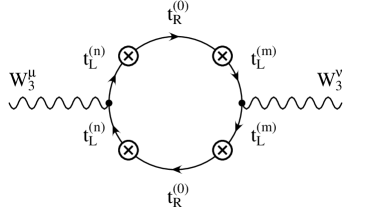
Figure 2: Representative lowest order contributions to the $T$ parameter from fermionic KK loop diagrams. The crosses represent insertions of the Higgs VEV. The corresponding $W^{+}$-$W^{-}$ graphs are neglected in the limit $m_{t}\gg m_{b}$.

In the presence of brane kinetic terms, both diagrams become finite due to the decoupling of the heavier KK modes. From Eqs. (21) and (23) we see that, for $c_{f}\neq 1/2$, for example, the couplings are given by

$$\lambda_{t_{L}^{(n)},t_{R}^{(0)}}\equiv\lambda_{n0}=\sqrt{\frac{2kL}{1+(1-2c_{Q})\alpha_{Q}k+\alpha_{Q}^{2}k^{2}x_{Q^{n}}^{2}}}\,a_{t}\frac{\lambda_{5}}{L}~{},$$ (40)

when a single KK mode and a zero mode are involved [$a_{t}$ is defined in Eq. (38)], and

$$\lambda_{t_{L}^{(n)},t_{R}^{(m)}}\equiv\lambda_{nm}=\sqrt{\frac{2kL}{1+(1-2c_{Q})\alpha_{Q}k+\alpha_{Q}^{2}k^{2}x_{Q^{n}}^{2}}}\sqrt{\frac{2kL}{1+(1-2c_{t})\alpha_{t}k+\alpha_{t}^{2}k^{2}x_{t^{m}}^{2}}}\,\frac{\lambda_{5}}{L}~{},$$ (41)

for the couplings among KK modes. Imposing that the the top mass be reproduced determines $\lambda_{5}/L$ from Eq. (37). We see that indeed the heavier KK modes couple more weakly to the brane. When $c_{f}=1/2$ one should use the general expressions for the KK mode wavefunctions, Eq. (24), although the approximate expressions, Eqs. (40) and (41), in the limit $c_{f}\rightarrow 1/2$ give a very good approximation to the $c_{f}=1/2$ case (within a few percent).

For $\alpha_{Q}k\sim\alpha_{t}k$ of order a few, the decoupling of the higher KK modes is very efficient and the contribution from the first KK level is an excellent approximation to the full tower. In addition, for $c_{Q}=1/2$, $c_{t}=0$ and $\alpha_{Q,t}k\sim$ a few, the diagram with $t_{R}$ zero modes dominates over that with $t_{R}$ KK modes. Thus, we may approximate the complete fermionic contribution to $\Delta T$ as,

$$\Delta T_{t}\approx\left(\frac{\lambda_{10}}{\lambda_{t}}\right)^{2}\left(\frac{m_{t}}{m^{(1)}_{t_{L}}}\right)^{2}\left[\frac{N_{c}}{16\pi s^{2}c^{2}}\left(\frac{m_{t}}{m_{Z}}\right)^{2}\right]\left\{\frac{4}{3}\left(\frac{\lambda_{10}}{\lambda_{t}}\right)^{2}+4\left[2\log\left(\frac{m^{(1)}_{t_{L}}}{m_{t}}\right)-\frac{3}{2}\right]\right\}~{},$$ (42)

where the term in square brackets is the SM top contribution, which is of order one. The terms in the curly brackets are the expressions for graphs containing two $t_{L}^{(1)}$ and one $t_{L}^{(1)}$ lines, respectively. This expression is a good approximation to the entire KK fermionic contribution for $\alpha k\begin{array}[]{c}\sim\vspace{-21pt}\\ >\end{array}3$. For smaller $\alpha$, there are relevant contributions from the $t_{R}$ KK modes. For the choice $\alpha_{Q}k=\alpha_{t}k=5$, $kL=30$, we find $\lambda_{t_{L}^{(1)},t_{R}^{(0)}}=2.37\,\lambda_{t}$ and $m^{(1)}_{t_{L}}=0.67\,\tilde{k}$. Taking, for example, $\tilde{k}=5~{}\textrm{TeV}$, results in $\Delta T\sim 0.25$. We note that the relevant coupling at the second KK level is $\lambda_{t_{L}^{(2)},t_{R}^{(0)}}=0.42\,\lambda_{t}$, while $m^{(2)}_{t_{L}}=3.94\,\tilde{k}$, from which it is easy to check that its effect is completely negligible. We conclude that the fermion localized kinetic terms are very efficient in suppressing these loop contributions to $T$, even for $c_{Q}=1/2$.

4.2 KK Gauge Boson Contributions

Integrating out the KK gauge bosons leads to important tree-level corrections to the weak gauge boson masses as well as to the couplings among the gauge fields and the quarks and leptons. These corrections arise from the fermion couplings to the KK gauge bosons and as a result of the mixing of the zero-mode weak gauge bosons with their KK modes, induced by the presence of the localized Higgs fields, as indicated in Fig. 3.

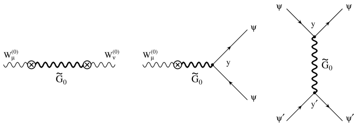
Figure 3: Tree-level contributions to the weak gauge boson masses, the gauge-fermion couplings, and four fermion operators, arising from the KK gauge bosons. $\widetilde{G}_{0}$ stands for the KK propagator at zero momentum, and the crosses represent insertions of the Higgs VEV squared (at $y=L$) whereas the small filled circles are insertions of the bulk $W$-$f$-$\overline{f}$ vertex, integrated over $y$.

Such effects can be efficiently handled with the aid of the propagator for the massive KK gauge fields, as explained in Ref. [20]. The KK summation can be done automatically by working in mixed position and 4D momentum space. Denoting this propagator by $\widetilde{G}_{p}(y,y^{\prime})$, where $p$ is the 4D momentum, the dominant low-energy corrections are all determined by the KK gauge propagator evaluated at zero momentum and the fermion zero-mode wavefunctions. In detail, the leading corrections may be computed in terms of $\widetilde{G}_{0}^{3}(L,L)$, $\widetilde{G}_{0}^{B}(L,L)$, and the quantities

$$G_{f}^{i} \equiv \int_{0}^{L}dy\widetilde{G}_{0}^{i}(L,y)|f^{(0)}(y)|^{2}\;\left(1+2\alpha_{f}\delta(y-L)\right)$$

$$G_{ff}^{i} \equiv \int_{0}^{L}dydy^{\prime}|f^{(0)}(y)|^{2}\widetilde{G}_{0}^{i}(y,y^{\prime})|f^{(0)}(y^{\prime})|^{2}~{}\;\left(1+2\alpha_{f}\delta(y-L)\right)\;\left(1+2\alpha_{f}\delta(y^{\prime}-L)\right),$$ (43)

where the superscript $i=3,B$ in the above quantities refer to the $W^{3}$ and $B$ gauge bosons of $SU(2)\times U(1)$, respectively, and $f^{(0)}(y)$ is the appropriate fermion zero-mode wavefunction, given in Eq. (13). The terms proportional to $\delta(y-L)$ represent the effects induced by the presence of the gauge-covariant brane kinetic terms of the fermions.

Observe that while the quantities $G_{f}$ and $G_{ff}$ serve to determine the corrections to the effective couplings of the zero-mode fermions to the weak gauge bosons and the induced four fermion operators, respectively, the corrections to the gauge boson masses are just a function of $\widetilde{G}_{0}(L,L)$. For instance, the $Z$ and $W$ masses are given by

$$m_{Z}^{2}=\frac{e^{2}\tilde{v}^{2}}{2s^{2}c^{2}}\left\{1+\frac{\tilde{v}^{2}}{2}[\widetilde{G}^{3}_{0}(L,L)+\widetilde{G}^{B}_{0}(L,L)]+{\cal{O}}(\frac{v^{4}}{k^{4}})\right\}~{}.$$ (44)

$$m_{W}^{2}=\frac{e^{2}\tilde{v}^{2}}{2s^{2}}\left\{1+\frac{\tilde{v}^{2}}{2}\widetilde{G}^{3}_{0}(L,L)+{\cal{O}}(\frac{v^{4}}{k^{4}})\right\}~{}.$$ (45)

In the above $\tilde{v}=ve^{-kL}\simeq 174~{}\textrm{GeV}$ is the Higgs field vacuum expectation value, and $s$ and $c$ represent the sine and the cosine of the tree-level weak mixing angle, $c=g/\sqrt{g^{2}+g^{\prime 2}}$ and $s=g^{\prime}/\sqrt{g^{2}+g^{\prime 2}}$.

Finally, the Fermi constant is given by

$$2\sqrt{2}G_{F}=\frac{1}{\tilde{v}^{2}}\left[1+\frac{\tilde{v}^{2}}{2}\left(2G_{f}^{3}-\widetilde{G}_{0}^{3}(L,L)-G_{ff}^{3}\right)+{\cal{O}}(\frac{v^{4}}{k^{4}})\right]~{},$$ (46)

where the $G_{ff}$ term represents non-oblique corrections.

In the cases we are going to analyze, with universal $c_{f}$ and $\alpha_{f}$ parameters, the only relevant non-oblique corrections to $m_{W}$ and the $Z$-pole observables come indirectly through the Fermi constant $G_{F}$. In this case, one can define effective precision electroweak parameters which determine $m_{W}$, as well as all Z-pole observables. Following Refs. [16, 20], and considering the expression of $G_{F}$, Eq. (46), it is possible to define these effective parameters $S_{\rm{eff}}$, $T_{\rm{eff}}$ and $U_{\rm{eff}}$, which are given by,

$$\alpha_{\rm em}S_{\rm{eff}} \approx 2\tilde{v}^{2}[s^{2}G_{f}^{3}+c^{2}G_{f}^{B}]+{\cal{O}}(\frac{v^{4}}{k^{4}})~{},$$

$$\alpha_{\rm em}T_{\rm{eff}} \approx \frac{\tilde{v}^{2}}{2}[2G_{f}^{B}-\widetilde{G}_{0}^{B}(L,L)+G^{3}_{ff}]+{\cal{O}}(\frac{v^{4}}{k^{4}})~{},$$ (47)

$$\alpha_{\rm em}U_{\rm{eff}} \approx -2s^{2}\tilde{v}^{2}G^{3}_{ff}+{\cal{O}}(\frac{v^{4}}{k^{4}})~{},$$

It is straightforward to find the explicit expression for $G_{f}$, $G_{ff}$ and $\widetilde{G}_{0}(L,L)$ in terms of the fundamental parameters of the theory. In the following, for simplicity, we ignore the UV brane kinetic terms. We comment on their effects below. In this case, one finds

$$\widetilde{G}_{0}(L,L)=-\frac{e^{2kL}g^{2}}{k^{2}}\frac{2k^{2}L^{2}-2kL+1}{4k(L+r_{IR})}~{}.$$ (48)

For further details of the calculation of the KK gauge propagator, $\widetilde{G}_{p}(y,y^{\prime})$, and its use to obtain the low-energy effective theory, refer to [16, 20].

The expressions for $G_{f}$ and $G_{ff}$ depend on the parameters $c_{f}$ and $\alpha_{f}$ through the fermion zero-mode wavefunctions, Eq. (13). The exact analytic expressions can be obtained in a straightforward manner, although the general results have a somewhat complicated dependence on $c_{f}$. However, in the case of interest here, where $c_{f}\begin{array}[]{c}\sim\vspace{-21pt}\\ >\end{array}1/2$, the expressions simplify considerably, up to exponentially small terms. We find

$\bullet$ For $c_{f}-\frac{1}{2}>1/2kL$:

$$G_{f} = \frac{e^{2kL}g^{2}}{k^{2}}\frac{kL-1-kr_{IR}+2k^{2}r_{IR}L}{4k(L+r_{IR})}~{},$$ (49)

$$G_{ff} = -\frac{e^{2kL}g^{2}}{k^{2}}\frac{2k^{2}r_{IR}^{2}+2kr_{IR}+1}{4k(L+r_{IR})}~{},$$ (50)

where $g$ is the (zeroth order) zero-mode gauge coupling. Note that the results in Eqs. (49) and (50) are independent of $c_{f}$ and $\alpha_{f}$.

$\bullet$ For $c_{f}=\frac{1}{2}$:

$$G_{f} = \frac{e^{2kL}g^{2}}{k}\frac{(2k^{2}L^{2}-2kL+1)(r_{IR}-\alpha_{f})}{4k^{2}(L+r_{IR})(L+\alpha_{f})}~{},$$ (51)

$$G_{ff} = -e^{2kL}g^{2}\frac{(2k^{2}L^{2}-2kL+1)(r_{IR}-\alpha_{f})^{2}}{4k^{3}(L+r_{IR})(L+\alpha_{f})^{2}}~{}.$$ (52)

Note that, in this case, $G_{f}$ may have either sign depending on the relative size of the gauge and fermion kinetic terms, $r_{IR}$ and $\alpha_{f}$. Also note that Eqs. (51) and (52) vanish when $r_{IR}=\alpha_{f}$. This is a consequence of the fact that, in this case, the fermion (see Eq. (12) for $f_{L}^{n}$) and gauge orthogonality conditions are identical, and the fact that for $c_{f}=1/2$ the fermion zero-mode wavefunction is flat and therefore proportional to the gauge zero mode wavefunction. Thus, the coupling of the zero-mode fermions to the higher KK gauge modes vanishes identically in this limit. This same fact was recently observed in warped extra-dimensional Higgsless models [22].

The precision electroweak observables depend on the relative size of the parameters $G_{f}$, $G_{ff}$ and $\widetilde{G}_{0}(L,L)$. In the limit of large values of $\alpha_{f}\gg L$, and for $c_{f}\leq 1/2$, the values of $G_{f}$, $G_{ff}$ tend to $\widetilde{G}_{0}(L,L)$. This result coincides with the one associated with fermions localized in the infrared brane. What happens in this case is that the physics is governed by the effects induced by the four dimensional brane kinetic terms, and propagation in the bulk becomes unimportant. The case of fermions localized in the infrared brane was already analyzed in [11, 15, 16].

Assuming that all quark and lepton bulk mass parameters, other than the right-handed top quark one, take values $c_{f}\simeq 1/2$ and that there is a common brane kinetic term coefficient $\alpha_{f}\equiv\alpha$, simple analytical expressions for $T_{\rm eff}$, $S_{\rm eff}$ and $U_{\rm eff}$ may be obtained:

$$T_{\rm eff}\simeq\frac{\pi}{c^{2}}\left(\frac{\tilde{v}}{\tilde{k}}\right)^{2}\left[\frac{k(L+2r_{IR}-\alpha)}{(1+r_{IR}/L)(1+\alpha/L)}\right]-\frac{U_{\rm eff}}{4s^{2}},$$ (53)

$$S_{\rm eff}\simeq 8\pi\left(\frac{\tilde{v}}{\tilde{k}}\right)^{2}\left[\frac{k(r_{IR}-\alpha)}{(1+r_{IR}/L)(1+\alpha/L)}\right],$$ (54)

$$U_{\rm eff}\simeq\frac{S_{\rm eff}}{2}\left[\frac{r_{IR}/L-\alpha/L}{1+\alpha/L}\right],$$ (55)

where, taking into account that $kL\simeq 30$, we have ignored terms of order $1/(kL)$. For moderate values of $k\alpha,kr_{IR}\ll kL$, the non-oblique corrections to the precision electroweak observables become small and, in particular, $U_{\rm eff}$, Eq. (55), become much smaller than $S_{\rm eff}$ and can be safely neglected in the description of the new physics corrections to the precision electroweak observables.

It is also useful to have an analytical approximation for the top-quark KK mode contribution to the parameter $T_{\rm eff}$, valid in the limits in which $m_{KK}/\widetilde{k}\begin{array}[]{c}\,\sim\vspace{-21pt}\\ <\end{array}1$ and $\alpha k\begin{array}[]{c}\sim\vspace{-21pt}\\ >\end{array}1$. In order to do this we computed the mass of the first KK mode of the left-handed top quark, for $c_{f}=1/2$, as a function of the brane kinetic term coefficient $\alpha$ (The same expression is valid for the mass of the first gauge field KK mass as a function of $r_{IR}$).

$$m^{(1)}_{t_{L}}\simeq ke^{-kL}\sqrt{8\frac{(1+\alpha/L)}{(1+4k\alpha)}}$$ (56)

while

$$\frac{\lambda_{t_{L}^{(1)},t_{R}^{(0)}}}{\lambda_{t}}\simeq 2\;\sqrt{\frac{kL}{1+4k\alpha}}.$$ (57)

Therefore, Eq. (42) reduces to

$$\Delta T_{t}\approx\left(\frac{kL}{1+\alpha/L}\right)\frac{m_{t}^{2}}{\widetilde{k}^{2}}\left[\frac{N_{c}}{16\pi s^{2}c^{2}}\left(\frac{m_{t}}{m_{Z}}\right)^{2}\right]\left\{\frac{8kL}{3(1+4k\alpha)}+2\log\left(\frac{8\tilde{k}^{2}(1+\alpha/L)}{m_{t}^{2}(1+4k\alpha)}\right)-3\right\}~{},$$ (58)

where, as before, the term in the square brackets is the SM contribution to $\Delta T$ from top, and is approximately equal to 1.2.

Up to now, we have neglected the effect of UV brane localized kinetic terms. We now briefly comment on their effects. Gauge and fermion localized UV kinetic terms have a mild impact on the spectrum. The effect of the UV terms in the KK masses amounts to replace $L$ by $L+\alpha_{UV}$ in Eq. (56) (or equivalently by $L+r_{UV}$ for the gauge boson KK masses). The main effect of UV kinetic terms is to shift the contribution of gauge and fermion KK modes to precision electroweak observables by quantities of order $r_{UV}/L$ ( or $\alpha_{UV}/L$). Hence, provided they are smaller than $L$, the inclusion of $r_{UV}$ and $\alpha_{UV}$ do not change the values of $\tilde{k}$ and the KK gauge boson and fermion masses consistent with experimental data in a significant way.

For completeness, we present the expressions of $\widetilde{G}_{0}(L,L)$ and $G_{f}$ for non-vanishing values of the UV kinetic terms. Keeping only dominant terms, for $kr_{IR}$ of order a few, $\widetilde{G}_{0}(L,L)$ reads [20],

$$\widetilde{G}_{0}(L,L)\simeq-\frac{g^{2}}{2\tilde{k}^{2}}\;\frac{k^{2}(L+r_{UV})^{2}}{k(L+r_{IR}+r_{UV})}~{}.$$ (59)

As anticipated, the comparison of this expression with the one presented in Eq. (48) shows corrections of order $r_{UV}/L$. Note that $\widetilde{G}_{0}(LL)$ is independent of the details associated with the fermion sector, and that it only affects the effective $T$ parameter. On the other hand, the size of $G_{f}$ and $G_{ff}$ are controlled by the IR parameters, $r_{IR}$ and $\alpha_{f}$, and receive corrections from $r_{UV}$ (gauge) and $\alpha_{UV}$ (fermion) kinetic terms of order $r_{UV}/L$ and $\alpha_{UV}/L$, respectively, but with a less straightforward dependence than the $\widetilde{G}_{0}(L,L)$ one. For instance, in the case $c_{f}=1/2$ and for $kr_{IR},k\alpha_{f}$ of order a few, the dominant contribution to $G_{f}$ reads

$$G_{f} \simeq \frac{g^{2}}{\tilde{k}^{2}}\;\frac{k(L+r_{UV})[r_{IR}(L+\alpha_{UV})-\alpha_{f}(L+r_{UV})]}{2(L+r_{IR}+r_{UV})(L+\alpha_{f}+\alpha_{UV})}~{},$$ (60)

Notice that the orthogonality condition, that ensures the cancellation of $G_{f}$, is fulfilled for $r_{IR}=\alpha_{f}$ and $r_{UV}=\alpha_{UV}$.

Finally, let us mention that for $k\alpha_{f}$ of order a few the expression of $\lambda_{t_{L}^{(1)},t_{R}^{(0)}}/\lambda_{t}$ for non-vanishing values of $\alpha_{UV}$ may be obtained by changing $L$ by $L+\alpha_{UV}$ in Eq. (57). Moreover, the contributions of $G_{ff}$ to $T$ and $U$ remain very small provided $k\,r_{IR}$ and $k\alpha_{IR}$ are less than order a few, even if $r_{UV}$, $\alpha_{UV}$ are as large as order $L$.

Sizable UV localized gauge kinetic terms appear, for instance, in the unification scenario analyzed in Ref. [20], where $r_{IR}^{B}+r_{UV}^{B}\simeq-(r_{IR}^{3}+r_{UV}^{3})\simeq L/3$. In this particular case, for moderate values of the IR kinetic terms, $kr_{IR}\begin{array}[]{c}\,\sim\vspace{-21pt}\\ <\end{array}2$ (taking $r_{IR}^{B}=r_{IR}^{3}=r_{IR}$), and $\alpha_{UV}=0$, one obtains corrections of about 30 percent to the gauge boson contributions to the $T$ parameter, while the correction to the $S$ parameter are smaller than 10 percent. One would then find corrections of about 10–15 percent for the values of $\tilde{k}$ consistent with the electroweak observables. Since the relation between the KK masses and $\tilde{k}$ is quite insensitive to the UV localized terms, this translates directly into a 10–15 percent correction to the KK masses. This should be compared with the effects induced by IR kinetic terms, that modify the relation between the lightest KK masses and $\tilde{k}$ in a much more crucial way, and control the value of the effective $S$ parameter, as well as the top-quark KK mode contributions to the $T$ parameter. Therefore, for simplicity, in the following section we shall restrict ourselves to the case of vanishing values of the UV kinetic terms.

4.3 Electroweak Fit

In this section, we will consider the case in which the values of $\alpha\,k$ and $r_{IR}k$ are of order of a few, and hence for vanishing values of the UV kinetic terms Eqs. (42), (53), (54) and (55) provide a good description to the dominant fermion and gauge boson contributions to the precision electroweak data. In this case, the model under consideration falls under the general class of theories in which there are only small corrections to the parameter $U$, while the corrections to $S$ and $T$ are sizable and of the order of the corrections associated with a heavy Higgs boson. One can therefore extract the allowed values of $S$ and $T$, by making a fit to the electroweak precision data under the assumption that all new physics contributions can be parametrized by these two parameters.

While making a fit to the electroweak data, one must choose a reference value for the Higgs boson mass, $m_{H_{\rm ref}}$, for which the SM gives $S=T=0$. One then obtains a countour in the $S$, $T$ plane indicating the allowed new physics contributions to the $S$ and $T$ parameters for that particular value of that Higgs mass. Had one chosen a different reference value for the Higgs mass, $m_{H}$, the allowed new physics contribution to $S$ and $T$ would be shifted by an amount equal (but of opposite sign) to the contribution to $S$ and $T$ obtained by the change of the Higgs mass from $m_{H_{\rm ref}}$ to $m_{H}$. This Higgs boson contribution to $S$ and $T$ is given by

$$S_{H}=\frac{1}{12\pi}\ln\left(\frac{m_{H}^{2}}{m_{H_{\rm ref}}^{2}}\right)\,,$$

$$T_{H}=-\frac{3}{16\pi c^{2}}\ln\left(\frac{m_{H}^{2}}{m_{H_{\rm ref}}^{2}}\right)\,.$$ (61)

We are interested in setting constraints on the masses of the fermion and gauge boson KK excitations, for arbitrary values of the Higgs boson mass. The LEP electroweak working group has recently extracted the allowed values of the $S$ and $T$ parameters coming from a fit to the electroweak precision data [23]. For a reference value of the Higgs boson mass $m_{H_{\rm ref}}=$ 150 GeV, they obtained

$$S\simeq 0.04\pm 0.10\,,$$

$$T\simeq 0.12\pm 0.10\,,$$ (62)

with $85\%$ correlation between the two parameters. Based on this information, in Fig. 4 we obtain the $95\%$ confidence level allowed region for the $S$ and $T$ parameters for three different values of the Higgs bosons mass $m_{H}=115,300$ and 800 GeV, respectively. Also shown in the Figure are the KK mode contributions to the $S$ and $T$ parameters for different values of $\alpha$ and $\tilde{k}$, for a value of the gauge field brane kinetic term $kr_{IR}\simeq 5$. We see that generically, a heavier Higgs boson mass allows for lower values of $\tilde{k}$, due to compensation between contributions to $T$ from the Higgs and the extra dimensional contributions. Values of $\tilde{k}$ as low as 4.5 TeV are consistent with experimental data. Note that for $\alpha k\sim r_{IR}k\sim 5$, the mass of the first KK modes are about $2/3\times\tilde{k}$, whereas for $\alpha k\sim 10$ the fermion first KK mode mass is approximately $1/2\times\tilde{k}$. Hence for these particular values of the IR kinetic terms, the lightest KK gauge boson and fermions masses may be as low as about 3 TeV and 2.3 TeV, respectively.

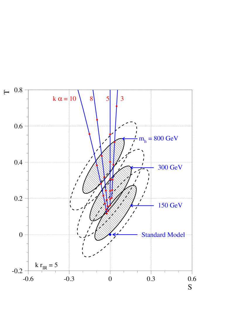
Figure 4: 95% and 68% allowed regions in the $S$-$T$ plane, for $kr_{IR}=5$, $r_{UV}^{3}=r_{UV}^{B}=0$, and different values of the Higgs boson mass. Also shown in the Figure is the KK mode contributions to the $S$ and $T$ parameters for different values of $\alpha$ and $\tilde{k}$, starting (at the lower end of each fixed $\alpha$ line) with $\tilde{k}=10$ TeV and decreasing in steps of 1 TeV for each dot.

5 Conclusions

Extra dimensional models provide an alternative solution to the gauge hierarchy problem. Among the different realizations of this idea, the Randall Sundrum model is perhaps the most attractive one. In particular the Randall Sundrum model with fermions and gauge bosons propagating in the bulk allows to address the question of unification of couplings and sets the framework for a possible understanding of flavor coming from the localization of the fermions in the bulk of the extra dimensional space.

In this article we have studied the impact of localized brane kinetic terms for the fermions in this scenario. The infrared brane kinetic terms repell the wavefunction of the heavy KK modes from the infrared brane where the Higgs field is localized and allows to solve the strong coupling problem of the top Yukawa sector and to minimize potentially dangerous flavor-violating effects. It is interesting to see that despite its underlying non-renormalizability, the extra dimensional theory already contains in itself a mechanism to suppress power-law corrections to brane couplings.

In the same spirit, a fermion brane kinetic term further renders the potential quadratically divergent contributions to the $T$ parameter finite and reduces the impact of the extra dimensional effects on the precision electroweak parameters. This allows all of the left-handed fermions to have bulk masses with $c\begin{array}[]{c}\sim\vspace{-21pt}\\ >\end{array}1/2$, and allows one to realize the attractive scenario in which the SM flavor hierarchies are (at least in part) generated by extra-dimensional geometry. Previous attempts have had larger corrections to the $Z$ coupling to bottom quarks, in contradiction with high precision measurements. In the end, KK masses as low as a few TeV are permitted, which could be discovered at the LHC.

Acknowledgements
 
Work at ANL is supported in part by the US DOE, Div. of HEP, Contract W-31-109-ENG-38. Fermilab is operated by Universities Research Association Inc. under contract no. DE-AC02-76CH02000 with the DOE. A. D.  is supported by NSF Grants P420D3620414350 and P420D3620434350 and also wants to thank the Theory Division of Fermilab and IFT Madrid for the kind invitation.

References

- [1] L. Randall and R. Sundrum, Phys. Rev. Lett. 83, 3370 (1999) [arXiv:hep-ph/9905221].
- [2] A. Pomarol, Phys. Rev. Lett. 85, 4004 (2000) [arXiv:hep-ph/0005293]. L. Randall and M. D. Schwartz, JHEP 0111, 003 (2001) [arXiv:hep-th/0108114]; Phys. Rev. Lett. 88, 081801 (2002) [arXiv:hep-th/0108115]; K. w. Choi, H. D. Kim and Y. W. Kim, JHEP 0211, 033 (2002) [arXiv:hep-ph/0202257]; JHEP 0303, 034 (2003) [arXiv:hep-ph/0207013]; W. D. Goldberger and I. Z. Rothstein, Phys. Rev. Lett. 89 (2002) 131601 [arXiv:hep-th/0204160]; Phys. Rev. D 68 (2003) 125011 [arXiv:hep-th/0208060]; Phys. Rev. D 68 (2003) 125012 [arXiv:hep-ph/0303158]; K. Agashe, A. Delgado and R. Sundrum, Nucl. Phys. B 643, 172 (2002) [arXiv:hep-ph/0206099]; R. Contino, P. Creminelli and E. Trincherini, JHEP 0210, 029 (2002) [arXiv:hep-th/0208002]; A. Falkowski and H. D. Kim, JHEP 0208, 052 (2002) [arXiv:hep-ph/0208058]; K. w. Choi and I. W. Kim, Phys. Rev. D 67, 045005 (2003) [arXiv:hep-th/0208071]; L. Randall, Y. Shadmi and N. Weiner, JHEP 0301, 055 (2003) [arXiv:hep-th/0208120]; A. Lewandowski, M. J. May and R. Sundrum, Phys. Rev. D 67, 024036 (2003) [arXiv:hep-th/0209050]; K. Agashe and A. Delgado, Phys. Rev. D 67, 046003 (2003) [arXiv:hep-th/0209212].
- [3] T. Gherghetta and A. Pomarol, Nucl. Phys. B 586, 141 (2000) [arXiv:hep-ph/0003129].
- [4] K. Agashe, A. Delgado and R. Sundrum, Annals Phys. 304, 145 (2003) [arXiv:hep-ph/0212028].
- [5] S. J. Huber, C. A. Lee and Q. Shafi, Phys. Lett. B 531, 112 (2002) [arXiv:hep-ph/0111465].
- [6] H. Verlinde, Nucl. Phys. B 580, 264 (2000); J. Maldacena, unpublished remarks; E. Witten, ITP Santa Barbara conference ‘New Dimensions in Field Theory and String Theory’, http://www.itp.ucsb.edu/online/susy_c99/discussion; S. Gubser, Phys. Rev. D 63, 084017 (2001); E. Verlinde and H. Verlinde, JHEP 0005, 034 (2000); N. Arkani-Hamed, M. Porrati and L. Randall, JHEP 0108, 017 (2001); R. Rattazzi and A. Zaffaroni, JHEP 0104, 021 (2001); M. Perez-Victoria, JHEP 0105, 064 (2001).
- [7] H. Georgi, A. K. Grant and G. Hailu, Phys. Lett. B 506, 207 (2001) [arXiv:hep-ph/0012379].
- [8] E. Pontón and E. Poppitz, JHEP 0106, 019 (2001) [arXiv:hep-ph/0105021].
- [9] M. Carena, T. M. P. Tait and C. E. M. Wagner, Acta Physica Polonica, B33, 2355 (2002) arXiv:hep-ph/0207056.
- [10] F. del Aguila, M. Perez-Victoria and J. Santiago, JHEP 0302, 051 (2003) [arXiv:hep-th/0302023].
- [11] C. Csaki, J. Erlich and J. Terning, Phys. Rev. D 66, 064021 (2002) [arXiv:hep-ph/0203034].
- [12] J. L. Hewett, F. J. Petriello and T. G. Rizzo, JHEP 0209, 030 (2002) [arXiv:hep-ph/0203091].
- [13] C. D. Carone, Phys. Rev. D 61, 015008 (2000) [arXiv:hep-ph/9907362]; A. Delgado, A. Pomarol and M. Quiros, JHEP 0001, 030 (2000) [arXiv:hep-ph/9911252]; D. E. Kaplan and T. M. Tait, JHEP 0111, 051 (2001) [arXiv:hep-ph/0110126]; S. J. Huber, arXiv:hep-ph/0303183. See also Ref. [12].
- [14] G. Burdman, Phys. Rev. D 66, 076003 (2002) [arXiv:hep-ph/0205329].
- [15] H. Davoudiasl, J. L. Hewett and T. G. Rizzo, arXiv:hep-ph/0212279.
- [16] M. Carena, E. Pontón, T. M. Tait and C. E. Wagner, arXiv:hep-ph/0212307.
- [17] K. Agashe, G. Perez and A. Soni, arXiv:hep-ph/0406101; arXiv:hep-ph/0408134.
- [18] K. Agashe, A. Delgado, M. J. May and R. Sundrum, JHEP 0308, 050 (2003) [arXiv:hep-ph/0308036].
- [19] Z. Chacko, M. A. Luty and E. Pontón, JHEP 0007, 036 (2000) [arXiv:hep-ph/9909248].
- [20] M. Carena, A. Delgado, E. Pontón, T. M. P. Tait and C. E. M. Wagner, Phys. Rev. D 68, 035010 (2003) [arXiv:hep-ph/0305188].
- [21] M. E. Peskin and T. Takeuchi, Phys. Rev. D 46, 381 (1992).
- [22] G. Cacciapaglia, C. Csaki, C. Grojean and J. Terning, arXiv:hep-ph/0409126.
- [23] http://lephiggs.web.cern.ch/LEPEWWG/.