MULTIPARTICLE PRODUCTION PROCESSES
FROM THE NONEXTENSIVE POINT OF VIEW

Abstract

We look at multiparticle production processes from the nonextensive point of view. Nonextensivity means here the systematic deviations in exponential formulas provided by the usual statistical approach for description of some observables like transverse momenta or rapidity distributions. We show that they can be accounted for my means of single parameter $q$ with $|q-1|$ being the measure of nonextensivity. The whole discussion will be based on the information theoretical approach to multiparticle processes proposed by us some time ago.

1 Introduction

The multiparticle production processes are usually approached first by means of statistical models [1] in order to make quick estimations of such parameters as ”temperature” $T$ or ”chemical potential” $\mu$. The quotation marks reflect the controversy in what concerns the applicability of such terms in the realm of hadronic production. Actually, as has been pointed long time ago [2], the fact that out of $N$ measured particles we usually observe only one of them is enough to make the relevant distribution (in transverse momentum $p_{T}$ or in rapidity $y$) being exponential:

$$f(X)\sim\exp\left[-\frac{X}{\Lambda}\right].$$ (1)

This is because the remain $N-1$ particles act as a ”heath bath” to the observed one and their action can be therefore summarized by a single parameter $\Lambda$. Identification of $\Lambda$ with temperature $T$ means that we assume that our system is in thermal equilibrium. However, in reality such ”heath bath” is not infinite and not homogenous (i.e., it can contain domains which differ between themselves). In such case single parameter $\Lambda$ is not sufficient to summarily describe its influence on the particle under consideration. One can regard it as being $X$-dependent and use the first two terms of its expansion around some value $X_{0}$ (instead of only $X_{0}$): $\Lambda\simeq\Lambda_{0}+a\cdot(X-X_{0})$. In this case distribution (1) becomes

$$f_{q}(X)\sim\exp_{q}\left[-\frac{X}{\Lambda_{0}}\right]\stackrel{{\scriptstyle def}}{{=}}\left[1-(1-q)\frac{X-X_{0}}{\Lambda_{0}}\right]^{\frac{1}{1-q}}\qquad{\rm where}\qquad q=1+a.$$ (2)

In case when $X$ is energy $E$ and $\Lambda$ is temperature $T$ the coefficient $a$ is just the reverse heat capacity, $a=1/C_{V}$ [3]. Such phenomenon is called nonextensivity and with $q$ being the nonextensivity parameter. Notice that for $q\rightarrow 1$ (or for $a\rightarrow 0$) $f_{q}(X)$ becomes $f(X)$.

In next Section we shall look at this problem from the information theory of view using Shannon and Tsallis information entropies. Confrontation with experimental data will be provided in Section 3. Section 4 will contain summary and conclusions.

2 Information theory and multiparticle production processes

Let us consider situation, which happens quite often in physics realm. Suppose that experimentalist provided us with some new data. Immediately these data are subject of interest to a number of theoretical groups, each of them quickly proposing their own distinctive and unique (in what concerns assumptions and physical concepts) explanation. Albeit disagreeing on physical concepts they are all fairly successful in what concerns fitting data at hand. The natural question which arises is: which of the proposed models is the right one? The answer is: to some extend - all of them! This is because experimental data are providing only limited amount of information and all models are simply able to reproduce it. To quantify this reasoning one has to define the notion of information and to do this, one has to resort to Information Theory (IT). It is based on Shannon information entropy

$$S=-\sum_{i}\,p_{i}\,\ln p_{i}\,,$$ (3)

where $p_{i}$ denotes probability distribution of interest. Notice that the least possible information, corresponding to the equal probability distribution of $N$ states (i.e., $p_{i}=1/N$), results in maximal entropy, $S=\ln N$. The opposite situation, when only one state is relevant, i.e., $p_{k}=1$ and $p_{i\neq k}=0$, results in the minimal entropy, $S=0$. Usually one always has some a priori information on experiment, like conservation laws and results of measurements, which is represented by a set of known numbers, $\langle R_{k}\rangle$. One is then seeking probability distribution $\{p_{i}\}$ such that:

• it tells us the truth, the whole truth about our experiment, what means that, in addition to be normalized, $\sum_{i}p_{i}=1$, it reproduces the known results, i.e.,

  $$\sum_{i}\,p_{i}\,R_{k}(x_{i})\,=\,\langle R_{k}\rangle\,;$$ (4)

• it tells us nothing but the truth about our experiment, i.e., it conveys the least information (only the information contain in this experiment).

To find such $\{p_{i}\}$ one has to maximize Shannon entropy under the above constraints (therefore this approach is also known as MaxEnt method). The resultant distribution has familiar exponential shape

$$p_{i}\,=\,\frac{1}{Z}\,\cdot\exp\left[-\sum_{k}\lambda_{k}\cdot R_{k}(x_{i})\right]\,.$$ (5)

Although it looks identical to the ”thermal-like” (Boltzmann-Gibbs) formula (1) there are no free parameters here because $Z$ is just normalization constant assuring that $\sum p_{i}=1$ and $\lambda_{k}$ are the corresponding lagrange multipliers to be calculated from the constraint equations (4).

It is worth to mention at this point [4] that the most probable multiplicity distribution $P(n)$ in the case when we know only the mean multiplicity $\langle n\rangle$ and that all particles are distinguishable is geometrical distribution $P(n)=\langle n\rangle^{n}/(1+\langle n\rangle)^{(n+1)}$ (which is broad in the sense that its dispersion is $D(n)\sim\langle n\rangle$). Additional knowledge that all these particles are indistinguishable converts the above $P(n)$ into Poissonian form, $P(n)=\exp(-\langle n\rangle)/n!$, which is the narrow one in the sense that now its dispersion is $D(n)\sim\sqrt{\langle n\rangle}$. In between is situation in which we know that particles are grouped in $k$ equally strongly emitting sources, in which case one gets Negative Binomial distribution [7] $P(n)=\Gamma(k+n)/\left[\Gamma(n+1)\Gamma(k)\right]\cdot\left(\frac{k}{\langle n\rangle}\right)^{k}/\left[1+\frac{k}{\langle n\rangle}\right]^{k+n}$.

The other noticeably example concerns the use of IT to find the minimal set of assumptions needed to explain all multiparticle production data of that time [8]. It turned out that all competing models like: multi-Regge, uncorrelated jet, thermodynamical, hydrodynamical etc., shared (in explicit or implicit manner), two basic assumptions:

• that only part $W=K\cdot\sqrt{s}$ ($0<K<1$) of the initially allowed energy $\sqrt{s}$ is used for production of observed secondaries (located in the center part of the phase space); in this way inelasticity $K$ found its justification [11], it turns out that $K\sim 0.5$;

• that transverse momenta of produced particles are limited and the resulting phase space is effectively one-dimensional (dominance of the longitudinal phase space).

All other assumptions specific for a given model turned out to be just spurious.

Suppose now that some new data occur which disagree with the previously established form of $\{p_{i}\}$. In IT approach it simply signals additional information to be accounted for. This can be done either by adding a new constraint (resulting in new $\lambda_{k+1}$) or by checking whether one should not use $\exp_{q}(...)$ rather than $\exp(...)$. This brings to IT the notion of nonextensivity introduced before and is connected with freedom in choosing the form of information entropy. The point is that there are systems which experience long range correlations, memory effects, which phase space has fractal character or which exhibit some intrinsic dynamical fluctuations of the otherwise intensive parameters (making them extensive ones, like $T$ in the example above). Such systems are truly small because the range of changes is of the order of their size. In this case the Shannon entropy (3) is no longer good measure of information and should be replaced by some other measure. Out of infinitely many possibilities [9, 10] we shall choose Tsallis entropy defined as

$$S_{q}\,=\,-\frac{1}{1-q}\sum_{i}\,\left(1-p_{i}^{q}\right),$$ (6)

which, as can be easily shown, goes over to Shannon form (3) for $q\rightarrow 1$. To get the $\{p_{i}\}$ one proceeds in the same way as before but modifying the constraint equation in the following way,

$$\sum_{i}\,\left[p_{i}\right]^{q}\,R_{k}(x_{i})\,=\,\langle R^{(q)}_{k}\rangle.$$ (7)

This leads to formally the same formula for $p_{i}=p^{(q)}_{i}$ as in eq. (5) but with $Z\rightarrow Z_{q}$ and $\exp(...)\rightarrow\exp_{q}(...)_{q}$. (For our purpose this method is sufficient and there is no need to use the more sophisticated approach exploring the so called escort probabilities formalism, see [11]). Because such entropy is nonextensive, i.e., $S_{q(A+B)}=S_{qA}+S_{qB}+(1-q)S_{qA}\cdot S_{qB}$ (see [9] for more details), the whole approach takes name nonextensive (Tsallis) statistics. Nonextensivity parameter $q$ accounts summarily for the all possible sources of nonextensivity mentioned before, however, here we shall be interested here only in intrinsic fluctuations present in the system. This is because in this case, as was demonstrated in [12], parameter $q$ is measure of such fluctuations, namely for system described by eq. (2) one has that

$$q\,=\,1\,\pm\,\left[\left\langle\left(1/\Lambda\right)^{2}\right\rangle\,-\,\left\langle 1/\Lambda\right\rangle^{2}\right]/\left\langle 1/\Lambda\right\rangle^{2}.$$ (8)

In what follows we shall argue that multiparticle production data on both transverse momentum $p_{T}$ and rapidity $y$ distributions can be interpreted as showing effects of such fluctuations.

3 Confrontation with experimental data

One should stress that what we present here is not a model but only least biased and most probable (from the point of view of information theory) distributions describing available data and accounting for constraints emerging either from the conservation laws or from some dynamical input (which in this way is subjected to confrontation with data). Suppose that we have mass $M$, which hadronizes into $N$ secondaries and hadronization is taking place in $1-$dimensional longitudinal phase space. Dynamics is hidden here in the fact that decay is into $N$ particles and that transverse momenta of particles are limited so one can use their transverse mass $\mu_{T}$ (suppose that we are not interested for a moment in details of the transverse momentum distribution). Once this is settled IT gives us clear prescription what to do:

• Look for single particle distribution in longitudinal phase space taken as $y-$space and written as suitable probability distribution,

  $$f_{N}(y)\,=\,\frac{1}{N}\cdot\frac{dN}{dy}\,=\,\frac{1}{\sigma_{N}N}\int d^{2}p_{T}\frac{Ed\sigma}{d^{3}p}.$$ (9)

• Maximize the following entropy functional

  $$S\,=\,-\int^{Y_{M}}_{-Y_{M}}dy\,f_{N}(y)\cdot\ln\left[f_{N}(y)\right],$$ (10)

  under conditions that $f_{N}(y)$ is properly normalized and that one conserves energy (because of the symmetry of our problem the momentum will be satisfied automatically; no more information will be used):

  $$\int^{Y_{M}}_{-Y_{M}}\!\!\!f_{N}(y)=1\quad{\rm and}\quad\int^{Y_{M}}_{-Y_{M}}\!\!\!dyE\cdot f_{N}(y)=\mu_{t}\int^{Y_{M}}_{-Y_{M}}\!\!\!dyf_{N}(y)\cosh y=\frac{M}{N}.$$ (11)

As result one obtains that the most probable (and least biased) rapidity distribution is

$$f_{N}(y)\,=\,\frac{1}{Z}\cdot\exp\left[-\beta\cdot\cosh y\right]\quad{\rm where}\quad Z=\int^{Y_{M}}_{-Y_{M}}\!\!\!dy\exp\left[-\beta\cdot\cosh y\right]$$ (12)

and where $\beta=\beta(M,N)$ is obtained by solving eq. (11). The $y-$space is limited to

$$y\in(-Y_{M},Y_{M}),\quad Y_{M}=\ln\left\{\frac{M^{\prime}\mu_{t}}{2\mu_{T}}\left[1+\left(1-\frac{4\mu_{T}^{2}}{M^{\prime 2}}\right)^{1/2}\right]\right\},~{}~{}M^{\prime}=M-(N-2)\mu_{T}.$$

The following points should be remembered:

• For $N=2$ both particles must be at the ends of the phase space, i.e., $f_{2}(y)=\frac{1}{2}\left[\delta(y-Y_{M})+\delta(y+Y_{M})\right]$, therefore formally $\beta(M,2)=-\infty$.

• Between $N=2$ and $N\simeq N_{0}=2\ln N_{max}$ (where $N_{max}=M/\mu_{T}$) $\beta$ is negative and approaches zero only for $N=N_{0}$. Therefore only for $N=N_{0}$ we have $f_{N}(y)=const$, i.e., the famous Feynman scaling.

• For $N>N_{0}$ additional particles have to be located near the middle of phase space to in order to minimize energy cost of their production. As result $\beta>0$ now, in fact (see [4] for details) for some ranges of $<E>=M/N$ quantity $\bar{\beta}=\beta<E>$ remains approximately constant. Needles to say that for $N\rightarrow N_{max}$ all particles have to stay as much as possible at the center and therefore $\beta(M,N\rightarrow N_{max})\rightarrow+\infty$ whereas $f_{N\rightarrow N_{max}}(y)\rightarrow\delta(y)$.

Figure 1: Left panel: examples of rapidity distributions for different nonextensivities. Right panel: the energy dependence of the NB parameter $1/k$ (line) together with results for the nonextensivity $|q-1|$ obtained when fitting $pp$ and $\bar{p}p$ data at different energies (points) - see the top-left panel of Fig. 2.

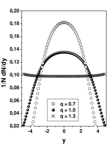
For nonextensive approach the only changes to be performed is to replace $\exp(...)$ by $\exp_{q}(...)_{q}$ in the way explained before. In addition $N_{0}\rightarrow N^{(q)}_{0}=\left(2\ln N_{max}\right)^{q}$. The changes in the shapes of $f_{q}(y)$ function for different values of $q$ are shown in Fig. 1. Notice that for $q>1$ one enhances tails of distribution and at the same time reduced its height. For $q1$ the effect is opposite (in this case there is kinematical constraint on the allowed phase space, namely it must conform to the condition that $1-(1-q)\beta_{q}\mu_{T}\cosh y\geq 0$. In fact in [15] we have found that we can fit reasonably well data on $\bar{p}p$ [16] with $q$ being the only parameter. Resultant $q<1$, which was cutting off the available phase space was there playing effectively the role of inelasticity of reaction mentioned before.

Figure 2: The most characteristic examples of comparison with data on rapidity distributions for different reactions. Top-left panel: the best fits to $pp$ and $\bar{p}p$ data [16] using nonextensive approach (cf. [11]). The resulting values of the $q$ parameters are shown above in Fig. 1. Top-right panel: fits to NA49 data for negatively charged pions produced in central $PbPb$ collisions at different energies [18] (cf. [5]). The best fit for $17.3$ GeV is, however, for two extensive sources located at $y=\pm\Delta y=0.83$ in rapidity (total inelasticity in this case is $K=0.58$). Bottom-left panel: fits to PHOBOS data for the most central $Au+Au$ collisions [19] (cf., [20]). Bottom-right panel: rapidity spectra measured in $e^{+}e^{-}$ annihilations at $91.2$ GeV [21] (dotted line is for $K_{q}=1$ and $q=1$ whereas full line is our fit with $K_{q}=1$ and $q=0.6$, see [20, 22]).

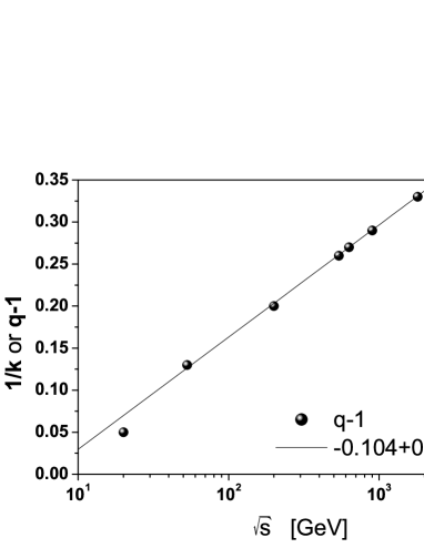
We repeated attempt to fit $\bar{p}p$ (and this time also $pp$) data [16] again but this time accountig properly for inelasticity (which was now free parameter to be deduced from data) and also for other possible fluctuations which hadronizing process offers us and which were represented by parameter $q$. We shall not discuss here the inelasticity issue (see [11] for details and further references) but concentrate on the $q$ parameter. In Fig. 1 we show the values of this parameter obtained for different energies compared with the values of the parameter $k$ of Negative Binomial distribution (NB) taken for different energies from existing data [17]. The agreement is perfect what prompted us to argue that parameter $q$ is accounting for a new bit of information, so far unaccounted for, namely that in addition to the mean multiplicity which was our input parameter there are other data [17] showing the whole multiplicity distributions, in particular showing their NB character. Actually this conjecture is supported by the observation [7] that NB can be obtained from Poisson distribution once one allows for fluctuations in its mean value $\bar{n}$ proceeding according to gamma distribution, namely

$$P(n)\,=\,\int_{0}^{\infty}d\bar{n}\frac{e^{-\bar{n}}\bar{n}^{n}}{n!}\cdot\frac{\gamma^{k}\bar{n}^{k-1}e^{-\gamma\bar{n}}}{\Gamma(k)}=\frac{\Gamma(k+n)}{\Gamma(1+n)\Gamma(k)}\cdot\frac{\gamma^{k}}{(\gamma+1)^{k+n}}$$ (13)

where $\gamma=\frac{k}{\langle\bar{n}\rangle}$ and $\frac{1}{k}=\frac{\sigma^{2}(n_{ch})}{\langle n_{ch}\rangle^{2}}-\frac{1}{\langle n_{ch}\rangle}$. Assuming now that these fluctuations contribute to nonextensivity defined by the parameter $q$, i.e., that $D(\bar{n})=q-1$ one gets that

$$q\,=\,1\,+\,\frac{1}{k},$$ (14)

what we do observe (cf. also [23]).

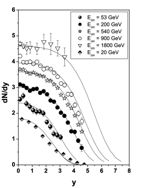
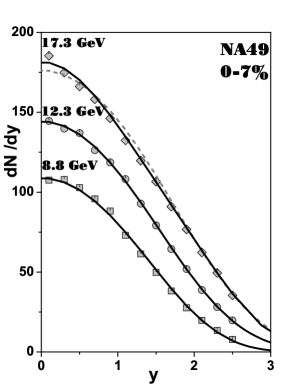
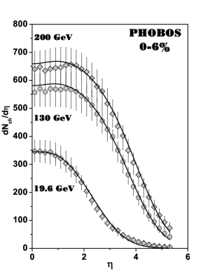
The next two panels show comparison with $AA$ data taking at SPS (NA49) and RHIC (PHOBOS) energies. The NA49 data can be fitted with $q=1.2$, $1.16$ and $1.04$ going from top to bottom and so far we do not have plausible explanation for these number. However, it should be stressed that at highest energy two component extensive source is preferable. The PHOBOS data with $q=1.27$, $1.26$ and $1.29$ going from top to bottom. Extensive fits do not work here at all. The example of $e^{+}e^{-}$ data clearly show that in this case there is some new information we did not accounted for. In this case the whole energy must be used but only $q<1$ fit (cutting-off a part of phase space) can be regarded as a fair one. But even then we cannot obtain minimum at $y=0$. It looks like we have two sources here separated in rapidity (two jets of QCD analysis) but of no statistical origin (rather connected with cascading) [22].

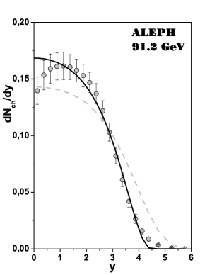
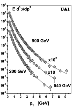
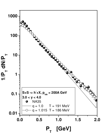
Let us now proceed to examples of $p_{T}$ distributions, see Fig. 3. Both $\bar{p}p$ data at high energies and nuclear data at lower energies are shown. They all can be fitted only with $q>1$ (for details see [5] and [26]. The characteristic feature is that now values of $q$ are much smaller than those obtained fitting data in longitudinal phase space. We shall not pursuit this problem here referring to discussion in [5]. Instead we shall concentrate on the nuclear data (right panel) and stress here that these data can, in our opinion, be connected with fluctuations of temperature mentioned at the beginning. In fact the $q=1.015$ obtained here fluctuation of $T$ of the order $\Delta T/T\simeq 0.12$, which do not vanish with increasing multiplicity [12]. In fact they are fluctuations existing in small parts of the hadronic system with respect to the whole system rather than of the event-by-event type, for which $\Delta T/T\sim 0.06/\sqrt{N}\rightarrow 0$ for large $N$. Such fluctuations are potentially very interesting because they provide a direct measure of the total heat capacity of the system, $C$, because

$$\frac{\sigma^{2}(\beta)}{\langle\beta\rangle^{2}}\stackrel{{\scriptstyle def}}{{=}}\frac{1}{C}=q-1.$$ (15)

In fact, because $C$ grows with the volume $V$ of reaction we expect that $q(hadronic)>q(nuclear)$ which seems to be indeed observed (cf., for example, Fig. 3).

Figure 3: Transverse momentum spectra showing nonextensive character. Left panel: fits to $p_{T}$ spectra from UA1 experiment on $\bar{p}p$ collisions [24]. Here $q=1.11$, $1.105$ and $1.095$ for energies decreasing from $900$ to $200$ GeV, respectively (cf., [11]). Right panel: fit to $p_{T}$ spectra from $S+S$ collisions [25] (cf., [26]). Notice that in this case $q=1.015$ only, i.e., it is smaller less than for $\bar{p}p$ case, see eq. (15).

4 Summary and conclusions

We have demonstrated that large amount of data on multiparticle production can be quite adequately described by using tools from information theory, especially when allowing for its nonextensive realization based on Tsallis entropy. We have argued that nonextensivity parameter $q$ entering here can, in addition to the temperature parameter $T$ of the usual statistical approaches, provide us valuable information on dynamical fluctuations present in the hadronizing systems. Such information can be very useful when searching for phase transition phenomena, which should be accompanied by some special fluctuations of nonmonotonic character. It is therefore worth to end with saying that some interesting fluctuations of this sort seems to be already seen and investigated [27]. All that calls for some more systematic effort to describe existing data in terms of $(T,q)$ for different configurations and energies in order to find possible regularities in their system and energy dependencies and possible correlations between them.

References

- [1] Cf., for example: F. Becattini, Nucl. Phys. A702 (2002) 336; W. Broniowski and W. Florkowski, Acta Phys. Polon. B35 (2004) 779 and references therein.
- [2] L. Van Hove, Z. Phys. C21 (1985) 93 and C27 (1985) 135.
- [3] M.P. Almeida, Physica A325 (2003) 426.
- [4] G. Wilk and Z. Włodarczyk, Phys. Rev. D43 (1991) 794.
- [5] F.S. Navarra, O.V. Utyuzh, G. Wilk and Z. Włodarczyk, Physica A340 (2004) 467.
- [6] A.M. Teweldeberhan, H.G. Miller and R. Tegen, Int. J. Mod. Phys. E12 (2003) 395.
- [7] P. Carruthers and C.C. Shih, Int. J. Mod. Phys. A4 (1989) 5587.
- [8] Y.-A. Chao, Nucl. Phys. B40 (1972) 475.
- [9] C. Tsallis, in Nonextensive Statistical Mechanics and its Applications, S.Abe and Y.Okamoto (Eds.), Lecture Notes in Physics LPN560, Springer (2000) and Physica A340 (2004) 1 and references therein.
- [10] F. Topsœ, Physica A340 (2004) 11.
- [11] F.S. Navarra, O.V. Utyuzh, G. Wilk and Z. Włodarczyk, Phys. Rev. D67 (2003) 114002.
- [12] G. Wilk and Z. Włodarczyk, Phys. Rev. Lett. 84 (2000) 2770; Chaos, Solitons, Fractals 13 (2002) 581 and Physica A305 (2002) 227.
- [13] C. Beck and E.G.D. Cohen, Physica A322 (2003) 267.
- [14] C. Beck, Physica A286 (200) 164.
- [15] F.S. Navarra, O.V. Utyuzh, G. Wilk and Z. Włodarczyk, Nuvo Cim. C24 (2001) 725.
- [16] R. Baltrusaitis et al. (UA5), Phys. Rev. Lett. 52 (1993) 1380; F. Abe et al. (Tevatron), Phys. Rev. D41 (1990) 2330; C. De Marzo et al., Phys. Rev. D26 (1982) 1019 and D29 (1984) 2476.
- [17] C. Geich-Gimbel, Int. J. Mod. Phys. A4 (1989) 1527.
- [18] S.V. Afanasjev et al. (NA49 Collab.), Phys. Rev. C66 (2002) 054902.
- [19] B.B. Beck et al., Phys. Rev. Lett. 91 (2003) 052303.
- [20] F.S. Navarra, O.V. Utyuzh, G. Wilk and Z. Włodarczyk, Physica A344 (2004) 568.
- [21] R. Barate et al. (ALEPH Collab.), Phys. Rep. 294 (1998) 1.
- [22] F.S. Navarra, O.V. Utyuzh, G. Wilk and Z. Włodarczyk, Single particle spectra from Information Theory point of view, hep-ph/0312166; to be published in Nukleonika (2004).
- [23] M. Rybczyński, Z. Włodarczyk and G. Wilk, Nucl. Phys. (Proc. Suppl.) B122 (2003) 325.
- [24] C. Albajar et al. (UA1 Collab.), Nucl. Phys. B335 (1990) 261.
- [25] T. Alber et al., (NA35 Collab.), Eur. Phys. J. C2 (1988)239.
- [26] O.V. Utyuzh, G. Wilk and Z. Włodarczyk, J. Phys. G26 (2000) L39.
- [27] M. Rybczyński, Z. Włodarczyk and G. Wilk, Acta Phys. Polon. B35 (2004) 819.