hep-ph/0410340

Summary of the Activities of the Working Group I
on High Energy and Collider Physics

Naba K. Mondal, Saurabh D. Rindani, Pankaj Agrawal, Kaustubh Agashe, B. Ananthanarayan, Ketevi Assamagan, Alfred Bartl, Subhendu Chakrabarti, Utpal Chattopadhyay, Debajyoti Choudhury, Eung-Jin Chun, Prasanta K. Das, Siba P. Das, Amitava Datta, Sukanta Dutta, Jeff Forshaw, Dilip K. Ghosh, Rohini M. Godbole, Monoranjan Guchait, Partha Konar, Manas Maity, Kajari Mazumdar, Biswarup Mukhopadhyaya, Meenakshi Narain, Santosh K. Rai, Sreerup Raychaudhuri, D.P. Roy, Seema Sharma, Ritesh K. Singh

Abstract

This is a summary of the projects undertaken by the Working Group I on High Energy Collider Physics at the Eighth Workshop on High Energy Physics Phenomenology (WHEPP8) held at the Indian Institute of Technology, Mumbai, January 5-16, 2004. The topics covered are (i) Higgs searches (ii) supersymmetry searches (iii) extra dimensions and (iv) linear collider.

The projects undertaken in the Working Group I on High Energy and Collider Physics can be classified into the categories (i) Higgs searches (ii) supersymmetry searches (iii) extra dimensions and (iv) linear collider. The reports on the projects are given below under these headings.

1 Higgs searches

1.1 Potential of Associated Higgs Production in LHC through $\tau$-pair mode

Participants: P.Agrawal and K.Mazumdar

At LHC, the Standard Model Higgs production in association with W-boson, $pp\rightarrow~{}WH$ is very interesting, though in general the total production rate is dominated by gluon-gluon fusion process. There is a strong indication that the Higgs boson is not very heavy and the experimental search for Higgs mass, $m_{H}\leq 150$ GeV/c² is comparatively more difficult. In any case it is desirable to study all possibilities for detection of Higgs boson in this mass range to strengthen the significance of discovery via ‘golden’ modes. This has motivated us to probe less studied modes of Higgs boson decays via WH production. Once the Higgs boson is discovered at LHC these final states will have to be studied for confirmation anyway.

The LHC experiments, both CMS and ATLAS, have special trigger algorithm at the first level (LEVEL 1) based on calorimetric information for selecting hadronic decays of $\tau$ in the final state  [1]. The $tau$-decay modes of Supersymmetric Higgs bosons have been particularly studied for this purpose. The narrowness of a jet as in the case of hadronic tau decays has been utilised in discrimenating the transverse profile of jets. The tracker information is used at a later stage for decision at a higher level and hence leptonic decays of $\tau$ cannot be used for trigger. Of course the leptonic decays of W-boson (only electron and muon final states) can be chosen for trigger in inclusive isolated electron/muon mode. But the background is likely to be overwhelming in that case. Hence we try the possibility of triggering the signal with the taus from the Higgs decay. This situation can be effectively utilised for the decay mode $H\rightarrow\tau^{+}\tau^{-}$ in the Higgs boson mass range $m_{H}\leq 140$ GeV/c² where the branching ratio is not too small, though below 10%.

According to the ’trigger menu’ of CMS experiment there are two possibilities for events with at least one $\tau$ in the final state. For 95% efficiency of signal selection (SUSY Higgs decay to tau final state) the kinematic thresholds are as follows.
1.Inclusive $\tau$-jet with jet transverse energy $\geq$ 86 GeV.
2. Double $\tau$-jets with the transverse energy of each jet $\geq$ 59 GeV.
It remains to be checked through simulation the efficiency in the signal channel after these requirements. We need to study the spectrum of transverse momenta of the tau-jets for this.

Assuming that a reasonable fraction of events survive the trigger condition, we need to reconstruct the events. Since the tau decays will inherently be accompanied by missing energy due to the neutrinos, we choose to select the hadronic decays of W-boson. The W mass can be reconstructed from the jets not identified as tau-tagged. Since the taus are highly boosted, the neutrinos are expected to be almost collinear with the direction of missing transverse energy. The mass of the Higgs boson can be reconstructed from this missing transverse energy and the visible momenta of the tau jets.

The main SM background to this channel is WZ production with $Z\rightarrow\tau^{+}\tau^{-}$ and $W\rightarrow$ 2-jets. Discarding events for which the tau-pair invariant mass is within the Z-mass window, a good fraction of the background can be removed. We plan to make a study after detector simulation to evaluate the signal-to- background ratio. But the Higgs boson being a scalar as opposed to Z, some angular correlations between the tau-jets can be utilised. This may not be as easy as in the case with leptons of course and we plan to make a simulation study of this.

1.2 Probing the light Higgs window via charged Higgs decay at LHC in CP violating MSSM

Participants: K. Assamagan, Dilip Kumar Ghosh, Rohini M. Godbole and D.P. Roy

It is well known that all the observed CP violation in High Energy Physics can be accommodated in the CKM picture in terms of a single CP-violating phase. Unfortunately this amount of CP violation in the quark sector, is not sufficient to explain quantitatively the observed Baryon Asymmetry in the Universe. CP violation in the Higgs sector is a popular extension of the Standard Model, which can cure this deficiency. Of course, CP violation in the Higgs sector is possible only in Multi-Higgs doublet models, such as a general two Higgs doublet model (2HDM) or the MSSM. MSSM with complex phases in the $\mu$ term and soft trilinear SUSY breaking parameters $A_{t}$ (and $A_{b}$), can have CP violation in the Higgs sector even with a CP-conserving tree level scalar potential. In the presence of these phases, due to the CP-violating interactions of the Higgs boson with top and bottom squarks, the one loop corrected scalar potential will in general have nonzero off-diagonal entries mixing the CP–even (S) and CP–odd (P) states, ${\cal M}^{2}_{SP}$, in the $3\times 3$ neutral Higgs mass-squared matrix. After diagonalizing this one-loop corrected scalar potential one will then, in general, have three neutral Higgs boson eigenstates, denoted by $H_{1},H_{2}$ and $H_{3}$ in ascending order of masses, with mixed CP parities [2, 3, 4, 5, 6, 7]. Sizeable scalar-pseudoscalar mixing is possible for large $\mid\mu\mid$ and $\mid A_{t}\mid(>M_{SUSY})$. Such CP-violating phases can cause the Higgs couplings to fermions and gauge bosons to change significantly from their values at the tree-level [3, 5, 6].

Recently the OPAL Collaboration [8] has reported their results for the Higgs boson searches in the CP-violating MSSM Higgs sector using the parameters defined in the CPX scenario [6] using the CP-SuperH [9] as well as the FeynHiggs 2.0 [10]. They have provided exclusion regions in the $M_{H_{1}}-\tan\beta$ plane for different values of the CP-violating phases, assuming ${\rm arg}A_{t}={\rm arg}A_{b}={\rm arg}M_{\tilde{g}}=\Phi_{\rm CP}$, with $\Phi_{\rm CP}=90^{o},60^{o},30^{o}$ and $0^{o}$. The values of the various parameters in the CPX scenario are chosen so as to showcase the effects of CP violation in the Higgs sector of the MSSM. Combining the results of Higgs searches from ALEPH, DELPHI, L3 and OPAL, the authors in Ref.[11] have also provided exclusion regions in the $M_{H_{1}}-\tan\beta$ plane as well as $M_{H^{+}}-\tan\beta$ plane for the above set of parameters.

Both these analyses show that for phases $\Phi_{\rm CP}=90^{o}$ and $60^{o}$, LEP cannot exclude presence of a light Higgs boson for $\tan\beta\sim 4-5,M_{H^{\pm}}\sim 125-140$ GeV, $M_{H_{1}}\stackrel{{\scriptstyle<}}{{{}_{\sim}}}60$ GeV and $\tan\beta\sim 2-3,M_{H^{\pm}}\sim 105-130GeV,M_{H_{1}}\stackrel{{\scriptstyle<}}{{{}_{\sim}}}40$ GeV respectively. This happens mainly due to the reduced $H_{1}ZZ$ coupling, as the lightest Higgs $H_{1}$ is mostly a pseudoscalar. In the same region the $H_{1}t\bar{t}$ coupling is suppressed as well. As a result this particular region in the parameter space can not be probed at the Tevatron where the associated production, $W/ZH_{1}$ mode is the most promising one; nor can it be probed at the LHC as the reduced $t\bar{t}H_{1}$ coupling suppresses the inclusive production mode and the associated production modes $W/ZH_{1}$ and $t\bar{t}H_{1}$, are suppressed as well.

It is interesting to note that in the same parameter space where $H_{1}ZZ$ coupling is suppressed, $H^{+}W^{-}H_{1}$ coupling is enhanced because these two sets of couplings satisfy a sum-rule [9]. We have found that in these regions of parameter space, $H^{\pm}\to H_{1}W^{\pm}$ has a very large $(\sim 100\%)$ branching ratio. This feature motivated us to study the possibility of probing such a light Higgs scenario in CP-violating MSSM Higgs model through the process $pp\to t\bar{t}\to(bW^{\pm})(bH^{\mp})\to(b\ell\nu)(bH_{1}W)\to(b\ell\nu)(bb\bar{b})(jj)$ at LHC. Thus signal will consist of 3 or more b-tagged and 2 untagged jets along with a hard lepton and missing $p_{T}$. Similar studies have been done in the context of charged Higgs search in NMSSSM model [12].

We report results obtained from a parton level Monte Carlo. We merge two partons into a single jet if the separation $\Delta R=\sqrt{\left(\Delta\phi\right)^{2}+\left(\Delta\eta\right)^{2}}<0.4$. As a basic selection criteria we require:

1. $\mid\eta\mid<2.5$ for all jets and leptons, where $\eta$ denotes pseudo-rapidity,

2. $p_{T}$ of the hardest three jets to be higher than 30 GeV,

3. $p_{T}$ of all the other jets, lepton, as well as the missing $p_{T}$ to be larger than 20 GeV,

4. A minimum separation of $\Delta R=0.4$ between the lepton and jets as well as each pair of jets,

5. Three or more tagged $b$-jets in the final state assuming a $b$-tagging efficiency of $50\%$.

Figure 1: Variation of signal cross-section with $M_{H^{+}}$ $(a)$ and $M_{H_{1}}$ $(b)$ for the CP-violating phase $\Phi_{CP}=60^{o}$.

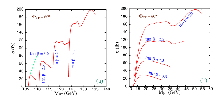
In Figure 1 we show the variation of signal cross-section with $M_{H^{+}}$ and $M_{H_{1}}$ for the CP-violating phase $\Phi_{\rm CP}=60^{o}$. We have used the CP-SuperH program [9] to calculate the masses and the couplings of the Higgses in the CPX scenario. The cross-section shown in the figure includes neither the $b$–tagging efficiency for the three and more jets (5/16), nor the $K$–factor corresponding to the NLO QCD corrections for the $t\bar{t}$ production $(\sim 1.4$–$1.5)$. Hence the numbers in the figure need to be scaled down by roughly a factor of two to get the signal cross-section. From Figure 1 one can see that the signal cross-section decreases with increase in $\tan\beta$. This can be explained by the fact that $H^{+}\to H_{1}W^{+}$ as well as $t\to bH^{+}$ branching ratio decreases with the increase in $\tan\beta$. The $t\to bH^{+}$ branching ratio does increase after showing a dip around $\tan\beta\sim 5-6$. However, we are not interested in such a high value of $\tan\beta$ in the present investigation as the loss of light Higgs signal due to $\not C\!\!P\hskip 2.84544pt$ in the Higgs sector is not significant for these higher values of $\tan\beta$.

Note that the signal events will be very striking due to the clustering of the $b\bar{b}$, $b\bar{b}W$ invariant masses at values corresponding to $M_{H_{1}}$ and $M_{H^{+}}$ respectively. Also the signal events will have simultaneous clustering of $b\bar{b}bW$ invariant mass around $m_{t}$.

         

Figure 2: Clustering of the $b\bar{b}$, $b\bar{b}W$ and $\bar{b}bbW$ invariant masses around $M_{H_{1}}$, $M_{H^{+}}$ and $m_{t}$. The parameters chosen for the signal are : CP-violating phase $\Phi_{CP}=60^{o}$, $\tan\beta=3$ and $M_{H^{+}}=107$ GeV.

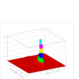
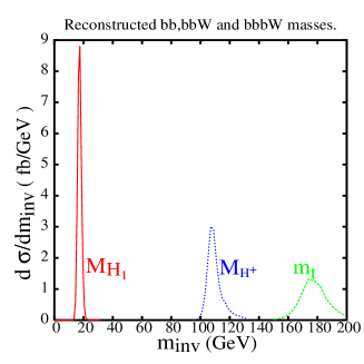
In Figure 2 we show in the left panel the 3-dimensional plot for the correlation between $m_{b\bar{b}}$ and $m_{b\bar{b}W}$ invariant mass distribution for $\Phi_{CP}=60^{o},\tan\beta=3$ and $M_{H^{+}}=107$ GeV. The light Higgs mass corresponding to this set of input parameter is 16.78 GeV. It is clear from Figure 2 that there is clustering at $M_{H_{1}}\equiv m_{b\bar{b}}$ and $M_{H^{+}}\equiv m_{b\bar{b}W}$. The right panel of the figure shows the same, in terms of cross-section distribution in $b\bar{b}$, $\bar{b}bW$ and $\bar{b}bbW$ invariant masses for the signal. This makes it very clear that the detectability of the signal is clearly controlled only by the signal size. It is clear from Figure 1 that indeed the signal size is healthy over the regions of interest in the parameter space. The clustering feature can be used to distinguish the signal over the standard model background. Thus using this process one can cover, at the LHC, a region of the parameter space in $\not C\!\!P\hskip 2.84544pt$ MSSM in the $\tan\beta-M_{H_{1}}$, plane which can not be excluded by LEP-2, where the Tevatron has no reach and which the LHC also can not probe if one does not use the process under discussion [13]. Of course, in view of the jetty final state, a more rigorous experimental simulation, including detector effects and hadronisation, will be useful to add further to the strength of our observation. Such a simulation is in progress and the results will be presented elsewhere.

2 Supersymmetry searches

2.1 Fermion polarization in sfermion decays as a probe of CP phases in the MSSM

Participants: Thomas Gajdosik, Rohini M. Godbole and Sabine Kraml

Introduction CP violation is one feature of the SM that still defies a fundamental theoretical understanding, even though all the observed CP violation in High Energy Physics can be accommodated in the CKM picture in terms of a single CP-violating phase. However, this amount of CP violation in the quark sector is not sufficient to explain quantitatively the observed Baryon Asymmetry in the Universe. CP violation in the Higgs sector is a popular extension of the Standard Model, which might cure this deficiency. MSSM with complex phases in the $\mu$ term and soft trilinear SUSY breaking parameters $A_{t}$ (and $A_{b}$), can affect the Higgs sector  [14, 15] through loop corrections. One can then have CP-violating effects even with a CP-conserving tree level scalar potential. It is still possible to be consistent with the non-observation of the electron EDMs (eEDM). This makes the MSSM with CP-violating phases a very attractive proposition. It has therefore been the subject of many recent investigations, studying the implications of these phases on neutralino/chargino production and decay [16], on the third generation of sfermions [17] as well as the neutral [15, 18] and charged [19] Higgs sector. In these studies, the gaugino mass parmaeter $M_{1}$ is also taken to be complex in addition to the nonzero phases mentioned above. It is interesting to note that CP-even observables such as masses, branching ratios, cross sections, etc., often afford more precise probes of these phases, thanks to the larger magnitudes of the effects as compared to the CP-odd/T-odd observables. The latter, however, are the only ones that can offer direct evidence of CP violation [16]. A recent summary of the progress in the area can be found in [20, 21] and references therein.

In this project, we address the issue of probes of these phases through a study of the third generation sfermions. A recent study in this context, in the $\tilde{t},\tilde{b}$ sector in the second of Ref. [17], demonstrates that it may be possible to determine the real and imaginary parts of $A_{t}(A_{\tau})$ to a precision of 2–3% (10–20 % for low $\tan\beta$ and 3–7% at large $\tan\beta$) from a fit of the MSSM Lagrange parameters to masses, cross sections and branching ratios at a future LC. In this project [21] we have explored the the longitudinal polarization of fermions produced in sfermion decays, i.e. $\tilde{f}\rightarrow f\tilde{\chi}^{0}$ and $\tilde{f}\rightarrow f^{\prime}\tilde{\chi}^{\pm}$ with $f(\tilde{f})$ a third generation (s)quark or (s)lepton, as a probe of CP phases.

The average polarization of fermions produced in sfermion decays carries information on the $\tilde{f}_{L}$–$\tilde{f}_{R}$ mixing as well as on the gaugino–higgsino mixing [22]. The polarizations that can be measured are those of top and tau; both can be inferred from the decay product(lepton angle and/or pion energy) distributions. The use of polarization of the decay fermions for studies of MSSM parameter determination was first pointed out and demonstrated in Ref. [22, 23]. An extension of these ideas for the CP-violating case and the phase dependence of the longitudinal fermion polarization had been mentioned in the studies of [20]. We provide, in this note, a detailed discussion of the sensitivity of the fermion polarization to the CP-violating phases in the MSSM.

Fermion polarization in $\tilde{f}\rightarrow f\tilde{\chi}^{0}$ decays

The sfermion interaction with neutralinos is ($i=1,2$; $n=1,...,4$)

$${\cal L}_{f\tilde{f}\tilde{\chi}^{0}} = g\,\bar{f}\,(a^{\,\tilde{f}}_{in}P_{R}+b^{\,\tilde{f}}_{in}P_{L})\,\tilde{\chi}^{0}_{n}\,\tilde{f}_{i}+{\rm h.c.}$$ (1)

Thus $a^{\,\tilde{f}}_{in}(b^{\,\tilde{f}}_{in})$ determine the amplitude for the production of $f_{L}(f_{R})$ in the decay $\tilde{f}_{i}\rightarrow f\tilde{\chi}^{0}_{n}$. The gaugino interaction conserves the helicity of the sfermion while the higgsino interaction flips it. In the limit $m_{f}\ll m_{\tilde{f}_{i}}$, the average polarization of the fermion coming from the above decay can therefore be calculated as [22]

$${\cal P}_{f}=\frac{Br(\tilde{f}_{i}\rightarrow\tilde{\chi}^{0}_{n}f_{R})-Br(\tilde{f}_{i}\rightarrow\tilde{\chi}^{0}_{n}f_{L})}{Br(\tilde{f}_{i}\rightarrow\tilde{\chi}^{0}_{n}f_{R})+Br(\tilde{f}_{i}\rightarrow\tilde{\chi}^{0}_{n}f_{L})}=\frac{|b_{in}^{\tilde{f}}|^{2}-|a_{in}^{\,\tilde{f}}|^{2}}{|b_{in}^{\tilde{f}}|^{2}+|a_{in}^{\,\tilde{f}}|^{2}}\,.$$ (2)

We obtain for the $\tilde{f}_{1}\rightarrow f\tilde{\chi}^{0}_{n}$ decay (omitting the overall factor $g^{2}$ and dropping the sfermion and neutralino indices for simplicity):

$$|b_{1n}|^{2}-|a_{1n}|^{2} = |h_{L}\cos\theta\,e^{-i\varphi}+f_{R}\sin\theta|^{2}-|f_{L}\cos\theta\,e^{-i\varphi}+h_{L}^{*}\sin\theta|^{2}$$ (3)

$$= (|h_{L}|^{2}-|f_{L}|^{2})\cos^{2}\theta-(|h_{L}|^{2}-|f_{R}|^{2})\sin^{2}\theta$$

$$+\,\sin 2\theta\,\big{[}\,{\cal R}e\,(f_{R}-f_{L})\,({\cal R}e\,h_{L}\cos\varphi+{\cal I}m\,h_{L}\sin\varphi)$$

$$\hskip 39.83385pt+\,{\cal I}m\,(f_{R}+f_{L})\,({\cal I}m\,h_{L}\cos\varphi-{\cal R}e\,h_{L}\sin\varphi)\,\big{]},$$

where $\theta,\varphi$ are the sfermion mixing angle and phase, and $f_{L},f_{R}$ and $h_{L},h_{R}$ are the gaugino and higgsino couplings of the left- and right-chiral sfermions respectively and contain the dependence on the phases in the gaugino–higgsino sector, $\phi_{1},\phi_{\mu}$. We see that the phase dependence of ${\cal P}_{f}$ is the largest for maximal sfermion mixing ($\theta_{\tilde{f}}=3\pi/4$) and if the neutralino has both sizeable gaugino and higgsino components. It is, moreover, enhanced if the Yukawa coupling $h_{f}$ is large. Furthermore, ${\cal P}_{f}$ is sensitive to CP violation even if just one phase, in either the neutralino or the sfermion sector, is non-zero. In particular, if only $A_{f}$ and thus only the sfermion mixing matrix has a non-zero phase, the phase-dependent term becomes

$$|b_{1n}|^{2}-|a_{1n}|^{2}\>\stackrel{{\scriptstyle\phi_{1}=\phi_{\mu}=0}}{{\sim}}\>h_{L}(f_{L}-f_{R})\sin 2\theta\cos\varphi\,.$$ (4)

The polarization ${\cal P}_{\!f}$, eq. (2), depends only on couplings but not on masses. For the numerical analysis we therefore use $M_{1}$, $M_{2}$, $\mu$, $\tan\beta$, $\theta_{\tilde{f}}$ and $\varphi_{\!\tilde{f}}$ as input parameters, assuming $\phi_{\mu}\approx 0$ to satisfy EDM constraints more easily: assuming cancellations for the 1-loop contributions and the CP-odd Higgs mass parameter $m_{A}>300$ GeV, 1-loop and 2-loop contributions to the electron EDM (eEDM), as well as their sum, stay below the experimental limit [24, 21] In order not to vary too many parameters, we use, moreover, the GUT relation $|M_{1}|=\frac{5}{3}\tan^{2}\theta_{W}M_{2}$ and choose $\tan\beta=10$ and $\theta_{\tilde{t}}=\theta_{\tilde{\tau}}=130^{\circ}$; i.e., large but not maximal mixing. The free parameters in this analysis are thus $M_{2}$, $|\mu|$, and the phases $\phi_{1}$, $\varphi_{\!\tilde{f}}$.

Figure 3: Average polarization of the tau lepton coming from $\tilde{\tau}_{1}\rightarrow\tau\tilde{\chi}^{0}_{1}$ decays in a) as a function of $M_{2}$ , in b) as a function of $|\mu|$. The full, dashed, dotted, dash-dotted, and dash-dot-dotted lines are for $(\phi_{1},\,\varphi_{\tilde{\tau}})=(0,\,0)$, $(0,\,\frac{\pi}{2})$, $(\frac{\pi}{2},0)$, $(\frac{\pi}{2},\,\frac{\pi}{2})$, and $(\frac{\pi}{2},\,-\frac{\pi}{2})$, respectively. $M_{2}$ and $\mu$ are taken to be real.

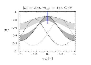
Figure 3 shows the average tau polarization in $\tilde{\tau}_{1}\rightarrow\tau\tilde{\chi}^{0}_{1}$ decays as functions of $M_{2}$ and $|\mu|$, for values consistent with the LEP constraints, for $\tan\beta=10$, $\theta_{\tilde{\tau}}=130^{\circ}$ and various choices of $\phi_{1}$ and $\varphi_{\tilde{\tau}}$. We find that the ${\cal P}_{\!\tau}$ is quite sensitive to CP phases for $|\mu|<M_{2}$, when $\tilde{\chi}^{0}_{1}$ has a sizeable higgsino component. Similarly the average top polarization in $\tilde{t}_{1}\rightarrow t\tilde{\chi}^{0}_{1}$ decays can be studied. We find that not only does it have a strong dependence on the CP phases if the neutralino has a sizeable higgsino component, but it is also significant when $|\mu|\sim M_{2}$, due to the much larger value of $m_{t}$ compared to $m_{\tau}$. Since at a future $e^{+}e^{-}$ linear collider (LC), one expects to be able to measure the tau polarization to about 3–5% and the top polarization to about 10% [25], the effects of CP-violating phases may well be visible in ${\cal P}_{\!t}$ and/or ${\cal P}_{\!\tau}$, provided $\mu$ is not too large.

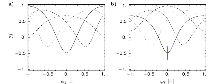
The phase dependence is further studied in Figure 4 where we show ${\cal P}_{\!t}$ as a function of $\phi_{1}$, for $M_{2}=380$ GeV, $|\mu|=125$ GeV and $\varphi_{\tilde{t}}=0$, $\frac{\pi}{2}$, $-\frac{\pi}{2}$ and $\pi$. Since for fixed $M_{2}$ and $|\mu|$ the $\tilde{\chi}^{0}_{1}$ mass changes with $\phi_{1}$, we show in addition in Fig. 4b ${\cal P}_{\!t}$ as a function of $\varphi_{\tilde{t}}$ for various values of $\phi_{1}$, with $|\mu|=125$ GeV and $M_{2}$ adjusted such that $m_{\tilde{\chi}^{0}_{1}}=100$ GeV. We thus see that if the neutralino mass parameters, $\tan\beta$ and $\theta_{\tilde{t}}$ are known, ${\cal P}_{\!t}$ can hence be used as a sensitive probe of these phases (although additional information will be necessary to resolve ambiguities and actually determine the various phases). The influence of uncertainties in the knowledge of the SUSY model parameters, can be studied by choosing the case of $M_{2}=380$ GeV, $|\mu|=125$ GeV and vanishing phases as reference point and assume that the following precisions can be achieved: $\delta M_{1}=\delta M_{2}=\delta\mu=0.5\%$, $\delta\tan\beta=1$, $\delta\theta_{\tilde{t}}=3.5^{\circ}$, and $\delta\phi_{1}=\delta\phi_{\mu}=0.1$. Varying the parameters within this range around the reference point and adding experimental resolution $\delta{\cal P}_{\!t}^{exp}\simeq 0.1$ in quadrature gives ${\cal P}_{\!t}=-0.48\pm 0.22$ at $\varphi_{\tilde{t}}=0$, indicated as an error bar in Fig. 4b. The figure shows that in this scenario ${\cal P}_{\!t}$ would be sensitive to $|\varphi_{\tilde{t}}|\;\raisebox{-3.87495pt}{$\textstyle\stackrel{{\scriptstyle\textstyle>}}{{\sim}}$}\;0.15\pi$. If more accurate measurements of the SUSY parameters should be available such that $\delta{\cal P}_{\!t}^{par}$ would be negligible compared to the experimental resolution of ${\cal P}_{\!t}$, then it would be possible to derive information on $A_{t}$ using the ${\cal P}_{\!t}$ measurement.

Figure 4: Average polarization of the top quark coming from $\tilde{t}_{1}\rightarrow t\tilde{\chi}^{0}_{1}$ decays for $\theta_{\tilde{t}}=130^{\circ}$, and $\tan\beta=10$: in a) as a function of $\phi_{1}$ for $M_{2}=225$ GeV and $|\mu|=200$ GeV; in b) as a function of $\varphi_{\tilde{t}}$ for $|\mu|=200$ GeV and $M_{2}$ adjusted such that $m_{\tilde{\chi}^{0}_{1}}=100$ GeV. The full, dashed, dotted, and dash-dotted lines are for $\varphi_{\tilde{t}}$ ($\phi_{1}$) $=0,{\textstyle\frac{\pi}{2}},-{\textstyle\frac{\pi}{2}},\pi$ in a (b). The error on ${\cal P}_{\!t}$ indicated by the vertical bar in b) has been estimated as described in the text.

Fermion polarization in $\tilde{f}\rightarrow f^{\prime}\tilde{\chi}^{\pm}$ decays

Analogous to the decay into a neutralino, eq. (2), the average polarization of the fermion coming from the $\tilde{f}_{i}\rightarrow f^{\prime}\tilde{\chi}^{\pm}_{j}$ decay ($i,j=1,2$) can be calculated once we know the $\tilde{f}_{i}f^{\prime}\tilde{\chi}^{\pm}_{j}$ coupling. These can be read off from the interaction Lagrangian:

$${\cal L}_{f^{\prime}\!\tilde{f}\tilde{\chi}^{\pm}} = g\,\bar{u}\,(l_{ij}^{\,\tilde{d}}\,P_{R}+k_{ij}^{\,\tilde{d}}\,P_{L})\,\tilde{\chi}^{+}_{j}\,\tilde{d}_{i}+g\,\bar{d}\,(l_{ij}^{\,\tilde{u}}\,P_{R}+k_{ij}^{\,\tilde{u}}\,P_{L})\,\tilde{\chi}^{+c}_{j}\,\tilde{u}_{i}+{\rm h.c.}$$ (5)

where $u$ ($\tilde{u}$) stands for up-type (s)quark and (s)neutrinos, and $d$ ($\tilde{d}$) stands for down-type (s)quark and charged (s)leptons. The average polarization is then given by

$${{\cal P}_{\!f}}^{\prime}=\frac{Br\,(\tilde{f}_{i}\rightarrow\tilde{\chi}^{\pm}_{j}f_{R}^{\prime})-Br\,(\tilde{f}_{i}\rightarrow\tilde{\chi}^{\pm}_{j}f_{L}^{\prime})}{Br\,(\tilde{f}_{i}\rightarrow\tilde{\chi}^{\pm}_{j}f_{R}^{\prime})+Br\,(\tilde{f}_{i}\rightarrow\tilde{\chi}^{\pm}_{j}f_{L}^{\prime})}=\frac{|k_{ij}^{\tilde{f}}|^{2}-|l_{ij}^{\,\tilde{f}}|^{2}}{|k_{ij}^{\tilde{f}}|^{2}+|l_{ij}^{\,\tilde{f}}|^{2}}\,.$$ (6)

Since only top and tau polarizations are measurable, we studied $\tilde{b}\rightarrow t\tilde{\chi}^{-}$ and $\tilde{\nu}_{\tau}\rightarrow\tau\tilde{\chi}^{+}$ decays. The latter case is especially simple because ${{\cal P}_{\!\tau}}^{\prime}$ depends only on the parameters of the chargino sector: A measurement of ${{\cal P}_{\!\tau}}^{\prime}$ may hence be useful to supplement the chargino parameter determination. However, only for the decay into the heavier chargino, the effect of a non-zero phase may be sizeable. Recall that unless huge cancellations are invoked, $\phi_{\mu}$ is severely restricted by the non-observation of the eEDM. Moreover, the measurement of $({{\cal P}_{\!\tau}}^{\prime})_{2}$ will be diluted by $\tilde{\nu}_{\tau}\rightarrow\tau\tilde{\chi}^{+}_{1}$ .

The top polarization in $\tilde{b}\rightarrow t\tilde{\chi}^{-}$ decays is more promising. Again we find that the phase dependence of ${{\cal P}_{\!t}}^{\prime}$ is proportional to $h_{b}\sin 2\theta_{\tilde{b}}$ and the amount of gaugino–higgsino mixing of the charginos; it will therefore be largest for $|M_{2}|\sim|\mu|$, $\theta_{\tilde{b}}=3\pi/4$ and large $\tan\beta$. Again, there is a non-zero effect even if there is just one phase in either the sbottom or chargino sector. Note, however, that the only CP phase in the chargino sector is $\phi_{\mu}$, which also enters the sfermion mass matrices. As a result, depending on values of $A_{b},\tan\beta$ and $\mu$, $\varphi_{\tilde{b}}$ and $\phi_{\mu}$ get related. For the sake of a general discussion of the phase dependence of ${{\cal P}_{\!t}}^{\prime}$ (and since $A_{b}$ is still a free parameter), we nevertheless use $\phi_{\mu}$ and $\varphi_{\tilde{b}}$ as independent input parameters. If $\phi_{\mu}$ and $\varphi_{\tilde{b}}$ have the same sign, the difference in ${{\cal P}_{\!t}}^{\prime}$ from the case of vanishing phases is larger than if they have opposite signs. In particular, we find ${{\cal P}_{\!t}}^{\prime}(\phi_{\mu}=-\varphi_{\tilde{b}})\sim{{\cal P}_{\!t}}^{\prime}(\phi_{\mu}=\varphi_{\tilde{b}}=0)$ over large regions of the parameter space. With an experimental resolution of the top polarization of about 10% this implies that in many cases $\varphi_{\tilde{b}}\sim-\phi_{\mu}$ cannot be distinguished from $\varphi_{\tilde{b}}=\phi_{\mu}=0$ by measurement of ${{\cal P}_{\!t}}^{\prime}$.

As an example of the phase dependence of the polarization ${{\cal P}_{\!t}}^{\prime}$ we show some of our results in Fig. 5

Figure 5: Average polarization of the top quark coming from $\tilde{b}_{1}\rightarrow t\tilde{\chi}^{-}_{1}$ decays as a function of $\varphi_{\tilde{b}}$, The full, dashed and dotted lines are for $\phi_{\mu}=0$, $\frac{\pi}{2}$ and $-\frac{\pi}{2}$, respectively, while for the dash-dotted lines $\phi_{\mu}=-\varphi_{\tilde{b}}$. The grey bands show the range of ${{\cal P}_{\!t}}^{\prime}$ due to varying $m_{b}$ within 2.5–4.5 GeV for the cases $\phi_{\mu}=0$ and $\phi_{\mu}=-\varphi_{\tilde{b}}$. The error bars show the estimated errors on ${{\cal P}_{\!t}}^{\prime}$ as described in the text.

which shows ${{\cal P}_{\!t}}^{\prime}$ as a function of $\varphi_{\tilde{b}}$, for $|\mu|=200$ GeV, $\tan\beta=10$, $\theta_{\tilde{b}}=140^{\circ}$, and various values of $\phi_{\mu}$. $M_{2}$ is chosen such that $m_{\tilde{\chi}^{\pm}_{1}}=155$ GeV (i.e. $M_{2}=225$ GeV for $\phi_{\mu}=0$). The range obtained by varying $m_{b}$ within 2.5–4.5 GeV is shown as grey bands for two of the curves, for $\phi_{\mu}=0$ and $\phi_{\mu}=-\varphi_{\tilde{b}}$. We estimate the effect of an imperfect knowledge of the model parameters in the same way as in the previous section. For $M_{2}=225\pm 1.125$ GeV, $|\mu|=200\pm 1$ GeV, $\tan\beta=10\pm 1$, $\theta_{\tilde{b}}=140\pm 3.4^{\circ}$ and $\phi_{\mu}=0\pm 0.1$, we get ${{\cal P}_{\!t}}^{\prime}=0.89\pm 0.06$ at $\varphi_{\tilde{b}}=0$. Varying in addition $m_{b}=2.5$–4.5 GeV gives ${{\cal P}_{\!t}}^{\prime}=0.89^{+0.06}_{-0.16}$. Adding a 10% measurement error on ${{\cal P}_{\!t}}^{\prime}$ in quadrature, we end up with ${\delta{\cal P}_{\!t}}^{\prime}=0.12$ ($0.19$) without (with) the $m_{b}$ effect. These are shown as error bars in Fig. 5. We see that the case of $\varphi_{\tilde{b}}=-\phi_{\mu}$ cannot be distinguished from $\varphi_{\tilde{b}}=\phi_{\mu}=0$ in this scenario. However, ${{\cal P}_{\!t}}^{\prime}$ turns out to be quite a sensitive probe of $\delta_{\phi}=\varphi_{\tilde{b}}+\phi_{\mu}$, i.e. the deviation from the ‘natural’ alignment $\varphi_{\tilde{b}}=-\phi_{\mu}$. In the example of Fig. 5, $|\delta_{\phi}|\;\raisebox{-3.87495pt}{$\textstyle\stackrel{{\scriptstyle\textstyle>}}{{\sim}}$}\;0.24\pi$ $(0.31\pi)$ can be resolved if $h_{b}$ is (not) known precisely, quite independently of $\phi_{\mu}$. Observing such a $\delta_{\phi}$ also implies a bound on $|A_{b}|$ of $|A_{b}|>1363$ $(1678)$ GeV. If the precision on $M_{2}$ and $|\mu|$ is 0.1% and $\tan\beta=10\pm 0.1$, we get $({\delta{\cal P}_{\!t}}^{\prime})^{par}=0.03$ at $\varphi_{\tilde{b}}=0$, so that the error is dominated by the experimental uncertainty. However, the resultant improvement in the sensitivity is limited to $|\delta_{\phi}|\;\raisebox{-3.87495pt}{$\textstyle\stackrel{{\scriptstyle\textstyle>}}{{\sim}}$}\;0.22\pi$ and $|A_{b}|>1294$ GeV.

Summary

We have investigated the sensitivity of the longitudinal polarization of fermions (top and tau) produced in sfermion decays to CP-violating phases in the MSSM. We have found that both ${\cal P}_{\!t}$ and ${\cal P}_{\!\tau}$ can vary over a large range depending on $\phi_{1}$ and $\varphi_{\tilde{t},\tilde{\tau}}$ (and also $\phi_{\mu}$, though we did not discuss this case explicitly) and may thus be used as sensitive probes of these phases. To this aim, however, the neutralino mass parameters, $\tan\beta$ and the sfermion mixing angles need to be known with high precision. Given the complexity of the problem, a combined fit of all available data seems to be the most convenient method for the extraction of the MSSM parameters. For the decays into charginos, the tau polarization in $\tilde{\nu}_{\tau}\rightarrow\tau\tilde{\chi}^{+}$ decays depends only little on $\phi_{\mu}$. ${{\cal P}_{\!\tau}}^{\prime}$ is hence not a promising quantity to study CP phases, but may be useful for (consistency) tests of the gaugino–higgsino mixing. The top polarization in $\tilde{b}\rightarrow t\tilde{\chi}^{-}$ decays, on the other hand, can be useful to probe $\phi_{\mu}$, $\varphi_{\tilde{b}}$ and/or $\delta_{\phi}=\phi_{\mu}+\varphi_{\tilde{b}}$ in some regions of the parameter space. The measurement of ${{\cal P}_{\!t}}^{\prime}$, revealing phases or being consistent with vanishing phases, may also constrain $|A_{b}|$. For a more detailed report of our investigations see [21].

2.2 Probing Non-universal Gaugino masses: Prospects at the Tevatron

Participants: Subhendu Chakrabarti, Amitava Datta and N. K. Mondal

Experiments at Fermilab Tevatron Run I [26] have obtained important bounds on the chargino-neutralino sector of the Minimal Supersymmetric extension of the Standard model using the clean trilepton signal. However, the analyses used the universal gaugino mass hypothesis at the GUT scale($M_{G}$) motivated by the minimal supergravity model(mSUGRA). On the other hand it is well known that even within the supergravity framework, non-universal gaugino masses may naturally arise if non-minimal gauge kinetic functions [27] are allowed. Specific values of gaugino masses at $M_{G}$ are somewhat model dependent. The main purpose of this work is to use the data from Tevatron Run I experiments to explore the possibility of constraining the chargino-neutralino sector of the MSSM without assuming gaugino mass universality. Rather than restricting ourselves to specific models, we shall focus our attention on the following generic hierarchies among the soft breaking parameters $M_{2}$ (the SU(2) gaugino mass parameter), $M_{1}$ ( the U(1) gaugino mass parameter) and the Higgsino mass parameter($\mu$) at the weak scale. Each pattern leads to a qualitatively different signal. We believe that this classification would lead to a systematic analysis of Run II data without assuming gaugino mass unification.

A) If $M_{1}<M_{2}<<\mu$, the clean trilepton signal trigerred by the decays ${\widetilde{\chi}_{1}}^{\pm}\rightarrow l^{\pm}\nu\widetilde{\chi}_{1}^{0}$ and $\widetilde{\chi}_{2}^{0}\rightarrow l^{+}l^{-}\widetilde{\chi}_{1}^{0}$ (l = e or $\mu$ ) is the dominant one. Here ${\widetilde{\chi}_{1}}^{\pm},\widetilde{\chi}_{1}^{0}$ and $\widetilde{\chi}_{2}^{0}$ are the lighter chargino (wino like), the lightest neutralino (bino like), assumed to be the lightest supersymmetric particle (LSP), and the second lightest neutralino (wino like) respectively. For $M_{2}\approx 2\times M_{1}$, one regains the spectrum in the popular mSUGRA model with radiative electroweak symmetry breaking, which usually guarantees relatively large $\mu$. If $M_{2}\approx\mu$ both ${\widetilde{\chi}_{1}}^{\pm}$ and $\widetilde{\chi}_{2}^{0}$ have strong higgsino components, but the trilepton signal may still be sizeable.

B) If $M_{1}<\mu\mathrel{\hbox to0.0pt{\raise 2.15277pt\hbox{$<$}\hss}{\lower 2.15277pt\hbox{$\sim$}}}M_{2}$, the $\widetilde{\chi}_{1}^{0}$ is bino like, the $\widetilde{\chi}_{2}^{0}$ has a strong higgsino component and the ${\widetilde{\chi}_{1}}^{\pm}$ is wino like. In this scenario the loop induced decay $\widetilde{\chi}_{2}^{0}\rightarrow\gamma\widetilde{\chi}_{1}^{0}$ occurs with a large branching ratio(BR), spoiling the trilepton signal. The signature of ${\widetilde{\chi}_{1}}^{\pm}-\widetilde{\chi}_{2}^{0}$ production is a $\gamma$ accompanied by standard model particles and large missing transverse energy.

C) If $M_{2}<M_{1}<<\mu$, the ${\widetilde{\chi}_{1}}^{\pm}$ and the $\widetilde{\chi}_{1}^{0}$ are wino like and approximately degenerate. Here spectrum is similar to the one predicted by the AMSB model. Since the chargino decays almost invsibly, special search strategies are called for[28].

D) If $\mu<<M_{1},M_{2}$, the ${\widetilde{\chi}_{1}}^{\pm},\widetilde{\chi}_{1}^{0}$ and $\widetilde{\chi}_{2}^{0}$ are approximately degenerate and higgsino like. As in C) special strategies for invisible/nearly invisible particles should be employed.

In this working group report we shall focus on scenario A). The trilepton signal has the added advantage that it is independent of the gluino mass $m(\mbox{$\widetilde{g}$})$ and hence independent of additional assumptions about the SU(3) gaugino sector.

The important parameters for the production of a ${\widetilde{\chi}_{1}}^{\pm}$ - $\widetilde{\chi}_{2}^{0}$ pair at the Tevatron are $M_{2},\mu$ , tan$\beta$ and the masses of the L type squarks belonging to the first generation $m_{\widetilde{q}_{L}}$, where q = u,d . The squark masses in question can safely be assumed to be degenerate, as is guaranteed by the $SU(2)_{L}$ symmetry, barring small calculable corrections due to SU(2) breaking D-terms. The parameter $M_{1}$ hardly affects the production cross section in scenario A) as will be shown below.

It may be noted that the bulk of the LEP constraints on the electroweak gaugino sector arise due to negative results from chargino search. The chargino pair production cross section at LEP is strongly suppressed for small sneutrino masses. The most conservative limits are, therefore, obtained for relatively light sleptons and sneutrinos.

Although the production cross section at Tevatron is independent of slepton/sneutrino masses, the leptonic BR’s of ${\widetilde{\chi}_{1}}^{\pm}$ and $\widetilde{\chi}_{2}^{0}$ depends on these masses. Since the BR’s in question are relatively small for heavy slepton/sneutrinos, the conservative limits correspond to such choices. Hence the information from Tevatron and LEP play complementary roles.

Using the event generator PYTHIA [29] and the kinematical cuts used in the CDF paper [26], we have simulated the trilepton signal for RUN I without assuming gaugino mass unification. For the purpose of illustration we present a subset of our results in table 1. The details will be presented else where[30].

Table 1:

$m_{{\widetilde{\chi}_{1}}^{\pm}}$(GeV)	$m_{\widetilde{\chi}_{1}^{0}}(GeV)$	$\sigma_{p}(pb)$	$BR$	$efficiency$
77.23	50.85	5.41	0.0127	0.035
76.25	38.0	5.77	0.0128	0.076
77.02	31.0	5.54	0.0129	0.081

For the calculations in table 1 we have set $\mu$ = - 400 GeV, tan $\beta$ = -6.0 and $\mbox{$m_{\mbox{$\widetilde{q}$}}$}=m_{\widetilde{\ell}}$ = 1.5 TeV. $m_{{\widetilde{\chi}_{1}}^{\pm}}$ is approximately fixed at a specific value using the parameter $M_{2}$ while the LSP mass is varied using the parameter $M_{1}$. The production cross section is denoted by $\sigma_{p}$ while BR is the branching ratio of the produced pair to decay into the clean trilepton channel.

We have restricted ourselves to a relatively low value of tan $\beta$ since large values of this parameter lead to light $\tau$ - sleptons and the final state is dominated by $\tau$ leptons instead of e or $\mu$. It follows from table 1 that for a given chargino mass the production cross section and the trilepton BR remains constant to a very good approximation for different choices of $M_{1}$ (or the $\widetilde{\chi}_{1}^{0}$ mass). The efficiency of the kinematical cuts on the other hand increases with lowering of $M_{1}$. Thus a lower limit on the mass of $\widetilde{\chi}_{1}^{0}$ as a function of the $m_{{\widetilde{\chi}_{1}}^{\pm}}$ is expected from the non-observation of any signal at Run I.

This limit may have important bearings on the viability of the LSP as the dark matter candidate. The current lower limit on $m_{\widetilde{\chi}_{1}^{0}}$ from LEP [31] crucially hinges on the gaugino mass unification hypothesis since it essestially originates from the chargino mass limit. Thus it is worthwhile to reexamine the limit without assuming gaugino mass unification. The indirect limit on $m_{\widetilde{\chi}_{1}^{0}}$ without gaugino mass unification is as low as 6 GeV [32]. It will also be interesting to see howfar this limit can be strengthened by data from direct searches at Run I and Run II.

3 Extra dimensions

3.1 Collider signals for Randall-Sundrum model (RS1) with SM gauge and fermion fields in the bulk

Participants: K. Agashe, K. Assamagan, J. Forshaw and R.M. Godbole

This work is based on the model in [33] to which the reader is referred for further details and for references.

Consider the Randall-Sundrum (RS1) model which is a compact slice of AdS₅,

$$ds^{2} = e^{-2k|\theta|r_{c}}\eta^{\mu\nu}dx_{\mu}dx_{\nu}+r_{c}^{2}d\theta^{2},\;-\pi\leq\theta\leq\pi,$$ (7)

where the extra-dimensional interval is realized as an orbifolded circle of radius $r_{c}$. The two orbifold fixed points, $\theta=0,\pi$, correspond to the “UV” (or “Planck) and “IR” (or “TeV”) branes respectively. In warped spacetimes the relationship between 5D mass scales and 4D mass scales (in an effective 4D description) depends on location in the extra dimension through the warp factor, $e^{-k|\theta|r_{c}}$. This allows large 4D mass hierarchies to naturally arise without large hierarchies in the defining 5D theory, whose mass parameters are taken to be of order the observed Planck scale, $M_{Pl}\sim 10^{18}$ GeV. For example, the 4D massless graviton mode is localized near the UV brane while Higgs physics is taken to be localized on the IR brane. In the 4D effective theory one then finds

$${\rm Weak~{}Scale}\sim M_{Pl}e^{-k\pi r_{c}}.$$ (8)

A modestly large radius, i.e., $k\pi r_{c}\sim\log\left(M_{Pl}/\hbox{TeV}\right)\sim 30$, can then accommodate a TeV-size weak scale. Kaluza-Klein (KK) graviton resonances have $\sim ke^{-k\pi r_{c}}$, i.e., TeV-scale masses since their wave functions are also localized near the IR brane.

In the original RS1 model, it was assumed that the entire SM (including gauge and fermion fields) resides on the TeV brane. Thus, the effective UV cut-off for the gauge, fermion and Higgs fields, and hence the scale suppressing higher-dimensional operators, is $\sim$ TeV. However, bounds from electroweak precision data on this cut-off are $\sim 5-10$ TeV, whereas those from flavor changing neutral currents (FCNC’s) (for example, $K-\bar{K}$ mixing) are $\sim 1000$ TeV. Thus, to stabilize the electroweak scale requires fine-tuning, i.e., even though RS1 explains the big hierarchy between Planck and electroweak scale, it has a “little” hierarchy problem.

A solution to this problem is to move the SM gauge and fermion fields into the bulk. Let us begin with how bulk fermions enable us to evade flavor constraints. The localization of the wave function of the massless chiral mode of a $5D$ fermion (identified with the SM fermion) is controlled by the $c$-parameter. In the warped scenario, for $c>1/2$ ($c<1/2$) the zero mode is localized near the Planck (TeV) brane, whereas for $c=1/2$, the wave function is flat. So, we choose $c>1/2$ for light fermions so that the effective UV cut-off $\gg$ TeV and thus FCNC’s are suppressed. Also this naturally results in a small $4D$ Yukawa coupling to the Higgs on TeV brane without any hierarchies in the fundamental $5D$ Yukawa couplings. Left-handed top and bottom quarks are close to $c=1/2$ (but $<1/2$) – we can show $c_{L}\sim 1/2$ is necessary to be consistent with $Z\rightarrow\bar{b}_{L}b_{L}$ for KK masses $\sim$ few TeV – whereas right-handed top quark is localized near the TeV brane to get $O(1)$ top Yukawa coupling. Furthermore, few ($3-4$) TeV KK masses are consistent with electroweak data ($S$ and $T$ parameters) provided we enhance the electroweak gauge symmetry in the bulk to $SU(2)_{L}\times SU(2)_{R}\times U(1)_{B-L}$, thereby providing a custodial isospin symmetry sufficient to suppress excessive contributions to the $T$ parameter.

We can show that in such a set-up (with bulk gauge fields) high-scale unification can be accommodated which is an added motivation for its consideration.

In this project, our goal is to identify/study collider signals for this model. We can show that the Higgs couplings to electroweak gauge KK modes are enhanced (compared to that of zero-modes, i.e., SM gauge couplings) by $\sim\sqrt{k\pi r_{c}}\sim 5-6$ since the Higgs is localized on the TeV brane and the wave functions of the gauge KK mode are also peaked near the TeV brane. Thus, longitudinal $W,Z$ (eaten Higgs component) fusion into electroweak gauge KK modes (with masses $\sim$ few TeV) is enhanced. In turn, these KK modes have sizable decay widths to longitudinal $W/Z$’s:

$$W_{long.}\;Z_{long.}\;(W_{long.}\;W_{long.}) \stackrel{{\scriptstyle g\sqrt{k\pi r_{c}}}}{{\longrightarrow}} W^{\pm\;(n)},Z^{(n)},\tilde{W}^{\pm\;(n)},Z^{\prime\;(n)}$$ (9)

$$\stackrel{{\scriptstyle g\sqrt{k\pi r_{c}}}}{{\longrightarrow}} W_{long.}\;Z_{long.}\;(W_{long.}\;W_{long.})$$

(here the subscript $(n)$ denotes a KK mode).

Note that the rise with energy of the $W_{long},Z_{long}$ cross section is softened by Higgs exchange, considerably below the energies of these resonances in longitudinal $W/Z$ scattering.

As per the AdS/CFT correspondence, this RS model is dual to a strongly coupled large-$N$ $4D$ conformal field theory (CFT) with $SU(3)_{c}\times SU(2)_{L}\times SU(2)_{R}\times U(1)_{B-L}$ global symmetry whose $SU(3)_{c}\times SU(2)_{L}\times U(1)_{Y}$ subgroup is gauged. A Higgs on the TeV brane corresponds to a composite of the CFT responsible for spontaneous breaking of $SU(2)_{L}\times SU(2)_{R}$ symmetry. That is, this model is dual to a particular type of a composite Higgs model. The electroweak gauge KK modes are techni-$\rho$’s in the dual interpretation. Thus, the enhanced coupling of Higgs to electroweak gauge KK modes was expected from their CFT dual interpretation as strongly coupled composites.

This is similar to technicolor models where one might anticipate a signal at the LHC in longitudinal $W/Z$ scattering for $\sim 2$ TeV techni-$\rho$’s. This process is illustrated in Figure 6. Whether there exists an observable signal for $3$ TeV gauge KK modes requires a calculation of the cross-section and a simulation of the process and associated backgrounds, which is in progress. In particular, one needs to determine whether the strong coupling to these new particles can compensate the suppression in rate due to the largeness of the resonant mass.

There are also possible signals with final states involving either two, three or four top quarks which are also illustrated in Figure 6. All three channels benefit from the fact that $t_{R}$ is strongly coupled, i.e. $\sqrt{k\pi r_{c}}$-enhanced, to the gluon and/or $W_{R}$ KK modes since its wave function is localized near TeV brane. The final channel illustrated in Figure 6 benefits from an enhanced Higgs-$t_{R}$-$b^{(n)}_{L}$ coupling $\sim\lambda_{t}f(c_{L})\sim\sqrt{10}$ (where $f(c_{L})\approx\sqrt{2/(1-2c_{L})}$ and $c\sim 0.4$ for $(t,b)_{L}$) which leads to $b_{L}^{(n)}$ production via longitudinal $W-t_{R}$ fusion. Such studies are underway.

,     ,

,      ,

Figure 6: Possible production mechanisms for KK states at the LHC

4 Linear collider

4.1 Transverse beam polarization and CP-violating triple-gauge-boson couplings in $e^{+}e^{-}\rightarrow\gamma Z$

Participants: B. Ananthanarayan, A. Bartl, Saurabh D. Rindani, Ritesh K. Singh

The project was to study the benefits from significant transverse polarization at the Linear Collider through the window of CP violation. Two of the members of the collaboration had recently studied the possibility of observing CP violation in the reaction $e^{+}e^{-}\rightarrow t\bar{t}$. It had been concluded in that study that CP violation only from (pseudo-)scalar (S) or tensor (T) type interactions due to beyond the standard model physics could be probed in the reaction when no final state polarization is observed, in the presence of transverse beam polarization. This result was obtained by generalizing certain results due to Dass and Ross from the 1970’s.

Discussions at WHEPP8 took place around the works cited above. It was realized that in a reaction involving self-conjugate neutral particles in the final state, transverse beam polarization could assist in probing CP violation that arose not necessarily from S and T currents. This stems from the fact that in the latter reaction, the matrix elements for the reaction receive contribution from the $t$ and $u$ channels. As a result, one project that was isolated was to carry out a full generalization of the results of Dass and Ross that were pertinent to $s-$channel reactions, to those which involve $t$ and $u$ channels.

As a first step therefore, one wished to study specific examples. For instance, the members of the collaboration wished to study the reaction $e^{+}e^{-}\rightarrow\gamma Z$ as an example. In particular, all beyond the standard model physics was assumed to arise from anomalous triple-gauge-boson couplings. The task was to compute the differential cross-section for the process in the presence of anomalous couplings and transverse beam polarization, and then to construct suitable CP-odd asymmetries. A numerical study was proposed to place suitable confidence limits on the anomalous couplings for realistic polarization and integrated luminosity at a design LC energy of $\sqrt{s}=500$ GeV.

After WHEPP8 the members of the collaboration carried out the project and the results are published in [34]. Two of the members of the collaboration have also considered more recently the most general gauge-invariant and chirality-conserving interactions that would contribute to CP violation in $e^{+}e^{-}\rightarrow\gamma Z$ [35].

Another possible example that was considered by the members of the collaboration was a reaction with a slepton pair in the final state. Work is yet to begin on this.

4.2 Decay lepton angular distribution in top production –
decoupling from anomalous $tbW$ vertex

Participants: Rohini M. Godbole, Manas Maity, Saurabh D. Rindani, Ritesh K. Singh

The project was to study the (in)dependence of decay lepton angular distribution, on any anomalous coupling in top-decay vertex, for different production processes of the top-quark. It is known in literature that the angular distribution of decay lepton, in pair production of top-quarks, is independent of the anomalous $tbW$ coupling to linear order. This result is independent of the initial state and hence valid for all colliders. Thus decay lepton angular distribution provides, at all colliders, a pure probe of possible anomalous interaction in the pair production of top-quarks, uncontaminated by any new physics in decay of top-quark. This result, though very attractive and useful, lacks a fundamental understanding. At WHEPP-8, we discussed possible approaches to understand the above said decoupling and explore the possibilities of extending this “decoupling theorem” to processes involving single top production and top pair production in $2\rightarrow 3$ processes. If the decoupling is observed in $2\rightarrow 3$, it possibly can be extended to $2\rightarrow n$ processes of top production.

4.3 Graviton Resonances in ${e^{+}e^{-}\rightarrow\mu^{+}\mu^{-}}$ with
beamstrahlung and ISR

Participants: Rohini M. Godbole, Santosh Kumar Rai and Sreerup Raychaudhuri

The next generation of high-energy $e^{+}e^{-}$ colliders [36, 37] will necessarily be Linear Colliders to avoid losses due to synchrotron radiation. However, as a linear collider will have single-pass colliding beams, the bunches constituting a beam would have to be focused to very small dimensions to get an adequate luminosity. This is an essential part of the design of all the proposed machines. The high density of charged particles at the interaction point would necessarily be accompanied by strong electromagnetic fields. The interactions of beam particles with the accelerating field generates the so-called initial state radiation (ISR), while their interactions with the fields generated by the other beam also generates radiation, usually dubbed Beamstrahlung[38].

Traditionally, ISR and Beamstrahlung have been considered nuisances which cause energy loss and disrupt the beam collimation. The energy-spread due to these radiative effects has led to a requirement of realistic simulations for physics processes which would require the knowledge of the energy spectrum of the colliding beams at the interaction point. The beam designs being considered are usually such that these effects are minimized.

In this note we argue that instead of just being a nuisance which we have to live with, photon radiation from initial states can actually be of great use in probing new physics scenarios under certain circumstances. As a matter of fact tagging with ISR photons has been used effectively in the LEP experiments, to search for final states which do not leave too much visible energy in the detectors; for example, a $\tilde{\chi}^{+}\tilde{\chi}^{-}$ (chargino) pair with $\tilde{\chi}^{+}$ and the LSP $\tilde{\chi}^{0}_{1}$ being almost degenerate[39]. Here, we look at a different aspect and usage of these radiative effects. To illustrate it we look at one of the simplest processes at an $e^{+}e^{-}$ collider, viz.

$$e^{+}~{}e^{-}\rightarrow X^{*}\rightarrow\mu^{+}~{}\mu^{-}$$

where $X$ can be either a massive scalar, vector or tensor. In the Standard Model, $X=\gamma,Z$. For any heavy particle $X$, there will be resonances in the $s$-channel process, observable as peaks in the invariant mass $M_{\mu^{+}\mu^{-}}$ distribution. At LEP, for example, this process was used to measure the $Z$-resonance line shape. In this note, we focus our attention on tensor particle resonances, the tensors being the massive Kaluza-Klein gravitons as predicted in the well-known braneworld model of Randall and Sundrum[40].

The central point in our argument is that it is very likely that the next generation linear colliders would run at one (or a few) fixed value(s) of centre-of-mass energy. For example, Tesla[36] is planned to run at $\sqrt{s}=500$ GeV and 800 GeV. However, the predicted massive graviton excitations of the Randall-Sundrum (RS) model may not lie very close to these energy values. Consequently, the new physics effect due to exchange of RS gravitons will be off-resonance and hence strongly suppressed. However, a spread in beam-energy would cause some of the events to take place at an effective (lower) centre-of-mass energy around the resonance(s) and hence provide an enhancement in the cross-section. A similar effect, for example, was observed in $Z$-resonances at LEP-1.5 and dubbed the ‘return to the $Z$-peak’. We, therefore, investigate ‘return to the graviton peak’ in the process $e^{+}~{}e^{-}\rightarrow\mu^{+}~{}\mu^{-}$.

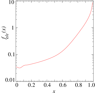
In our analysis of radiative effects we use the structure function formalism for ISR and Beamstrahlung developed in Refs.[41, 42]. Specifically, we use the expression for the electron spectrum function presented in [42]. Figure 7 shows the electron energy spectrum for the given design parameters for the linear collider at TESLA [36] running at $\sqrt{s}=800$ GeV. It is worth noting that the large spread in the distribution function is more due to Beamstrahlung than to ISR effects.[42]

Figure 7: Illustrating the effective electron luminosity at Tesla-800 as a function of $x=E_{e}/E_{\rm beam}$, the energy fraction of the electron after radiating a photon. The Beamstrahlung parameter is $\Upsilon=0.09$.

In the two-brane model of Randall and Sundrum, the Standard Model is augmented by a set of Kaluza-Klein excitations of the graviton, which behave like massive spin-2 fields with masses $M_{n}=x_{n}m_{0}$, where the $x_{n}$ are the zeroes of the Bessel function of order unity, $n$ is a non-negative integer and $m_{0}$ is an unknown mass scale close to the electroweak scale. Search possibilities for these gravitons at future $e^{+}e^{-}$ colliders, have been studied in the literature [43]. Experimental data from the Drell-Yan process at the Tevatron constrain $m_{0}$ to be more-or-less above 130 GeV[44]. Another undetermined parameter of the theory is the curvature of the fifth dimension, expressed as a fraction of the Planck mass $c_{0}={\cal K}/M_{P}$. Feynman rules for the Randall-Sundrum graviton excitations can then be read-off from the well-known Feynman rules given in Ref.[45] by making the simple substitution $\kappa\rightarrow 4\sqrt{2}\pi c_{0}/m_{0}$. Noting that the massive graviton states exchanged in the $s$-channel can lead to Breit-Wigner resonances, it is now a straightforward matter to calculate the cross-section for the process $e^{+}~{}e^{-}\rightarrow\mu^{+}~{}\mu^{-}$ and implement it in a simple Monte Carlo event generator.

Our numerical analysis has been performed for values $m_{0}=150$ GeV and $c_{0}=0.01$, which implies that the lightest ($n=1$) massive excitation has mass $M_{1}=574.5$ GeV, putting it well beyond the present reach of Run-II data at the Tevatron[44]. With this choice, however, the next excitation is predicted to have mass $M_{2}>1$ TeV, which puts it well beyond the reach of Tesla-800. We expect, therefore, to detect one, and only one, resonance. The value of $c_{0}$ has been chosen at the lower end of the possible range, since this leads to a longer lifetime for the Kaluza-Klein state and hence a sharper resonance in the cross-section. Following standard practice for linear collider studies, we eliminate most of the backgrounds from beam-beam interactions and two-photon processes by imposing an angular cut $10^{0}<\theta_{\mu^{\pm}}<170^{0}$ on the final-state muons. Some of our results are illustrated in Figure 8, which shows the binwise distribution of invariant mass $M_{\mu^{+}\mu^{-}}$ of the (observable) final state. In Figure 2($a$), we have plotted the distribution predicted in the Standard Model (SM). Figure 2($b$) shows the excess over the SM prediction expected in the Randall-Sundrum model and Figure 2($c$) shows the signal-to-background ratio.

Figure 8: Invariant mass distribution with (outlined histogram) and without (filled histogram) radiative effects. The figures show (a) the bin-wise cross-section $\sigma_{SM}$ for the SM background,  (b) the bin-wise excess cross-section $\sigma-\sigma_{SM}$ predicted in the RS model and  (c) the signal-to-background ratio $\sigma/\sigma_{SM}$.

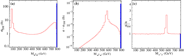
At a linear collider with fixed center-of-mass energies, all the events for the above process should be concentrated in a single invariant mass bin at $M_{\mu^{+}\mu^{-}}\sim\sqrt{s}$ in the lab frame. In Figure 2 these correspond to the solid (blue) bins in the $M_{\mu^{+}\mu^{-}}$ distribution. Comparison of Figures 2($a$) and 2($b$) show that the expected signal is very small indeed, about 1 in $10^{4}$. Consequently the ratio exhibited in Figure 2($c$) is almost precisely unity. This is because our parameter choice leads to a graviton of mass 574.5 GeV, and decay width of a few GeV, which is far away from the centre-of-mass energy $\sqrt{s}=800$ GeV.

The outlined (red) histograms in Figure 2 show the invariant mass distribution when radiative effects are included. It is immediately apparent that the invariant mass and hence the effective centre-of-mass energy $\sqrt{s^{\prime}}=M_{\mu^{+}\mu^{-}}$ is spread out from the beam energy $\sqrt{s}$. In ($a$), we can see a distinct peak at the lower end which represents ‘return to the $Z$-peak’. The cross-section for this peak is not as high as one might expect for a narrow resonance like the $Z$ because this corresponds to an extremely large value for the energy fraction $x$ taken away by the photon, for which the luminosity is extremely small. The shape of the rest of the histogram is simply a reflection of the electron luminosity shown in Figure 1. A similar phenomenon happens in ($b$) due to the large spread in the energy of the colliding beams. Here the radiative return to the resonant KK-graviton is quite apparent. In fact, excitation of the graviton resonance leads to a greatly enhanced cross-section, as this graph shows. The outlined (red) histogram in ($c$), shows the signal-to-background ratio. This ratio removes the $Z$-peak and clearly throws into prominence the graviton resonance, presenting us with a clear signal for a new resonant particle. To confirm that it is indeed a graviton, one must run various tests, such as plotting the angular distribution. These will be discussed in a forthcoming publication[46]. Note also that the method can be used with effect only for final states not involving strongly interacting particles, as two-photon processes can give rise to a substantial two-jet production for invariant masses quite a bit smaller than the nominal centre of mass energy of the collider [42].

It is thus clear that ISR and Beamstrahlung can play a non-trivial role in the identification of new physics effects. This is a positive feature of these radiative phenomena, which has not often been considered, and the main purpose of this work is to emphasize this aspect.

4.4 Probing R-parity Violating Models of Neutrino Mass at the Linear Collider

Participants: A.Bartl, S. P. Das, A. Datta, R. M. Godbole and D. P. Roy

The observation of neutrino oscillations and the measurement of oscillation parameters by the SUPERK collaboration [47] and others[48, 49] have established that at least two of the neutrino masses are non-zero albeit their magnitudes are several orders of magnitude smaller than that of the other fermions.

A natural explanation of the smallness of the neutrino masses is perhaps the most challenging task of current high energy physics. The see-saw mechanism [50] is certainly the most popular model. However, the simplest version of this model - a supersymmetric grand unified theory (SUSYGUT) of the grand desert type, which can also explain coupling constant unification[51], has practically no other crucial prediction for TeV scale physics. If an intermediate scale is allowed then both SUSY and non-SUSY GUTs, the latter being plagued by the notorious fine tuning problem, may serve the purpose. But there is no compelling reason within the framework of these models either for new physics at the TeV scale.

In contrast within the framework of R-parity violating (RPV) SUSY Majorana masses of the neutrinos can be generated both at the tree level and at the one loop level quite naturally. More importantly the physics of this mechanism is entirely governed by TeV scale physics (sparticle masses and couplings) which can in principle be verified at the next round of collider experiments.

Neutrino masses within the framework of RPV SUSY have been studied by several groups[52]. Such masses may arise both at the tree level as well as at the one loop level. As an example, we refer to [53], where upper bounds on RPV bilinear and trilinear terms were derived ( see tables III - VIII of [53] )using some simplifying assumptions about the R-parity-conserving (RPC) sector(see below).

In this working group project we try to further sharpen these predictions. We obtain several combinations of lepton number violating trilinear ($\lambda_{ijk},\lambda^{\prime}_{ijk}$, i,j,k = 1,2,3) and bilinear ($\mu_{i}$, i=1,2,3) couplings which are consistent with the current ranges of the oscillation parameters [54].

The squared mass differences of different neutrinos are defined as:

$$\Delta m^{2}_{sun}\equiv|\Delta m^{2}_{12}|,~{}~{}~{}~{}~{}~{}~{}\Delta m^{2}_{atm}\equiv|\Delta m^{2}_{23}|~{}~{}~{}.$$ (10)

where $\Delta m^{2}_{12}=m_{2}^{2}-m_{1}^{2}>0$ and $\Delta m^{2}_{23}=m_{3}^{2}-m_{2}^{2}$ assuming $m_{1}^{2}<m_{2}^{2}<m_{3}^{2}$.

The limits on them are

$$5\times 10^{-5}<\Delta m^{2}_{sun}(eV^{2})<10\times 10^{-5}$$

and

$$1\times 10^{-3}<\Delta m^{2}_{atm}(eV^{2})<4\times 10^{-3}.$$

Similarly the mixing angle constraints are

$$0.29<\tan^{2}\theta_{12}<0.82,$$

$$0.45<\tan^{2}\theta_{23}<2.3,$$

$$0.0<\tan^{2}\theta_{13}<0.05,$$

for solar, atmospheric and CHOOZ data [54] .

Since our results are basically illustrative, we employed the same simplifying assumptions as in [53].

• All masses and mass parameters in the RPC sector of the MSSM are $\approx$ 100 GeV.

• tan $\beta$ = 2

This leads to the following tree level and loop level mass matrices [53]:

$${\cal{M}}^{\mathrm{tree}}_{\nu_{ij}}=C\mu_{i}\mu_{j},$$ (11)

$${\cal{M}}^{\mathrm{loop}}_{\nu}=\!\!\left(\begin{array}[]{lll}K_{1}\lambda^{2}_{133}+K_{2}\lambda^{\prime 2}_{133}&K_{1}\lambda_{133}\lambda_{233}+K_{2}\lambda^{\prime}_{133}\lambda^{\prime}_{233}&K_{2}\lambda^{\prime}_{133}\lambda^{\prime}_{333}\\ K_{1}\lambda_{133}\lambda_{233}+K_{2}\lambda^{\prime}_{133}\lambda^{\prime}_{233}&K_{1}\lambda^{2}_{233}+K_{2}\lambda^{\prime 2}_{233}&K_{2}\lambda^{\prime}_{233}\lambda^{\prime}_{333}\\ K_{2}\lambda^{\prime}_{133}\lambda^{\prime}_{333}&K_{2}\lambda^{\prime}_{233}\lambda^{\prime}_{333}&K_{2}\lambda^{\prime 2}_{333}\end{array}\right),$$ (15)

where the constants are given by C $\approx$ 5.3 $\times$ $10^{-3}$ $GeV^{-1}$, $K_{1}$ $\approx$ 1.8 $\times$ $10^{-4}$ $GeV$ and $K_{2}$ $\approx$ 4.7 $\times$ $10^{-3}$ $GeV$. In [53] several scenarios were considered with five non-zero RPV couplings (see table III of [53]). For the purpose of illustration we consider scenario 1 where the non-vanishing parameters are the three $\mu$’s, $\lambda_{133}$ and $\lambda_{233}$.

Now we try to fit the above oscillation parameters by varying the above five parameters randomly subject to the existing bounds ( see table V of [53]; we have considered the MSW large mixing angle solution only). By generating 10000 sets of parameters we have obtained only 3 solutions in ( see, table 2 ). It is gratifying to note that even the rather loose constraints on the oscillation parameters currently available are sufficiently restrictive to yield a remarkably small set of solutions.

Table 2: Allowed RPV parameters consistent with the Neutrino data in [54]

Solution No.	$\mu_{1}(GeV)$	$\mu_{2}(GeV)$	$\mu_{3}(GeV)$	$\lambda_{133}$	$\lambda_{233}$
I	$1.1E-05$	$5.9E-05$	$8.2E-05$	$1.5E-04$	$1.9E-04$
II	$4.4E-06$	$6.5E-05$	$8.0E-05$	$1.4E-04$	$2.1E-04$
III	$8.0E-06$	$4.3E-05$	$7.9E-05$	$1.6E-04$	$2.1E-04$

Although $\tilde{\chi}_{1}^{0}$ (LSP) decay is generic in RPV models, the above examples illustrate that the branching ratios and the life time of the LSP, which we assume to be the lightest neutralino, will have very specific patterns if the oscillation constraints are imposed. In the scenario under consideration the allowed decay modes are:

$$(a)\tilde{\chi}_{1}^{0}\rightarrow e\tau\not\!\!{E_{T}},(b)\tilde{\chi}_{1}^{0}\rightarrow\mu\tau\not\!\!{E_{T}}~{}~{}and~{}~{}(c)\tilde{\chi}_{1}^{0}\rightarrow\tau\tau\not\!\!{E_{T}},$$ (16)

where the missing energy ($\not\!\!{E_{T}}$) is carried by the neutrinos. Charge conjugate modes are included in our analysis.

In Table 3 we have presented some LSP decay characteristics calculated by CompHEP[55] using the first two solutions in Table 2. We find that in order to distinguish solutions number I from II , the BR(a),(b) and the decay length have to be measured with accuracy better than 17.4%, 8.5% and 5.6% respectively.

Table 3: Lightest Neutralino decay branching ratios and decay lengths for the first two scenario of Table 2.

Solution. No.	BR	Decay length ( c $\times\tau$ in cm )
I	(a) 0.186
	(b) 0.323	35.82
	(c) 0.491
II	(a)0.156
	(b)0.352	37.66
	(c)0.492

Although our calculations were based on very specific assumptions there are reasons to believe that the restricted nature of the predictions of this model will continue to hold even without these assumptions. Improvement in the precision of the magnitudes of the oscillation parameters in the future long base line experiments will impose even tighter constraints on model parameters. For example, we have tested that the ranges of oscillation parameters in [53] (see Table I) based on old data lead to many more solutions.

Moreover measurements of superparticle masses, couplings and some of the Branching Ratios (BRs) will be available [56] from LHC within the first few years of its running, if SUSY exists. This may enable one to fix the constants C, $K_{1}$ and $K_{2}$ within reasonable ranges without additional assumptions. Precision measurements of LSP decay properties to verify the RPV models of neutrino mass seem to be a challenging, but perhaps feasible, task for the next linear collider (LC).

It is interesting to analyze the possible information one may seek at the Linear Collider to be able to do this job. In case it is the RPV version of SUSY that is realized in nature, even the LHC will offer a rather good measurement of the mass of the LSP, particularly if the $\lambda,\lambda^{{}^{\prime}}$ RPV couplings are the dominant ones. The LC will on the other hand will offer a chance for accurate measurement of the LSP mass as well as its life time provided the RPV couplings are large and the LSP has macroscopic decay length. We see from Table II, that for the particular solutions path lengths of a few cms. are possible for the LSP. Studies of possible accuracies of such measurement need to be performed. It will be possible to measure the mass of the decaying LSP at an LC using either the kinematic end point measurements and/or through the threshold scans. Very preliminary studies [57] of the possibilities of the mass measurements of the LSP in the production of $\tilde{\chi}_{1}^{0}\tilde{\chi}_{2}^{0},\tilde{\chi}_{1}^{+}\tilde{\chi}_{1}^{-}$, followed by the decay of the $\tilde{\chi}_{2}^{0},\tilde{\chi}_{1}^{\pm}$ and the LSP in the end exist. These studies need to be refined. Further, the LSP decay may also depend on the masses of the third generation sparticles and mixing, precision information for which may also be available only from the LC. These features as well as the possible interplay between the LHC and the LC to pin down RPV SUSY as the origin of neutrino mass need to be studied. Finally we note that if the $\lambda^{{}^{\prime}}$ couplings are indeed ${\cal O}(10^{-4})$ as required by models of $\nu$ mass [53], lighter top squark decays may provide additional evidence in favour of these models [58]

References

- [1] CMS Collaboration, The Data Acquisition and High-Level Trigger Project, Technical Design Report, CERN/LHCC 2002-26, CMS TDR 6.2, 2002.
- [2] A. Pilaftsis, Phys. Rev. D 58 (1998) 096010; Phys. Lett. B 435 (1998) 88.
- [3] A. Pilaftsis and C. E. Wagner, Nucl. Phys. B 553 (1999) 3.
- [4] D. A. Demir, Phys. Rev. D 60 (1999) 055006.
- [5] S. Y. Choi, M. Drees and J. S. Lee, Phys. Lett. B 481 (2000) 57.
- [6] M. Carena, J. Ellis, A. Pilaftsis and C. E. Wagner, Nucl. Phys. B 586 (2000) 92.
- [7] G. L. Kane and L. -T. Wang, Phys. Lett. B 488 (2000) 383.
- [8] OPAL Collaboration, hep-ex/0406057.
- [9] J. S. Lee, A. Pilaftsis, M. Carena, S. Y. Choi, M. Drees, J. R. Ellis and C. E. M. Wagner, Comput. Phys. Commun. 156 (2004) 283, [arXiv:hep-ph/0307377].
- [10] S. Heinemeyer, Eur. Phys. J. C 22 (2001) 521, [arXiv:hep-ph/0108059]; M. Frank, S. Heinemeyer, W. Hollik and G. Weiglein, arXiv:hep-ph/0212037.
- [11] M. Carena, J. Ellis, S. Mrenna, A. Pilaftsis and C. E. Wagner, Nucl. Phys. B 659 (2003) 145.
- [12] M. Drees, E. Ma, P. N. Pandita, D. P. Roy and S. K. Vempati, Phys. Lett. B 433 (1998) 346, [arXiv:hep-ph/9805242]; M. Drees, M. Guchait and D.P. Roy, Phys. Lett. B 471 (1999) 39.
- [13] M. Schumacher, Talk presented at the meeting on ’CP violation and Nonstandard Higgs Physics’, held at CERN, May 14-15,2004, http://agenda.cern.ch/fullAgenda.php?ida=a041761.
- [14] A. Dedes and S. Moretti, Phys. Rev. Lett. 84 (2000) 22, [arXiv:hep-ph/9908516]; Nucl. Phys. B 576 (2000) 29, [arXiv:hep-ph/990941]; S. Y. Choi, K. Hagiwara and J. S. Lee, Phys. Lett. B 529 (2002) 212 [arXiv:hep-ph/0110138];
- [15] M. Carena, J. Ellis, S. Mrenna, A. Pilaftsis and C. E. Wagner, Nucl. Phys. B 659 (2003) 145.
- [16] See, for some recent work, A. Bartl, H. Fraas, O. Kittel and W. Majerotto, arXiv:hep-ph/0402016, S. Y. Choi, M. Drees and B. Gaissmaier, arXiv:hep-ph/0403054.
- [17] See, for some recent work, A. Bartl, S. Hesselbach, K. Hidaka, T. Kernreiter and W. Porod, Phys. Lett. B 573 (2003) 153 [arXiv:hep-ph/0307317]; A. Bartl, S. Hesselbach, K. Hidaka, T. Kernreiter and W. Porod, arXiv:hep-ph/0311338.
- [18] F. Borzumati, J. S. Lee and W. Y. Song, arXiv:hep-ph/0401024.
- [19] E. Christova, H. Eberl, W. Majerotto and S. Kraml, Nucl. Phys. B 639 (2002) 263, Erratum-ibid. B 647 (2002) 359 [arXiv:hep-ph/0205227];
- [20] S. Heselbach, Talk presented at the International Linear Collider Workshop, 2004, Paris.
- [21] T. Gajdosik, Rohini M. Godbole and S. Kraml, arXiv-ph/0405167.
- [22] M. M. Nojiri, Phys. Rev. D 51 (1995) 6281 [arXiv:hep-ph/9412374].
- [23] M. M. Nojiri, K. Fujii and T. Tsukamoto, Phys. Rev. D 54, 6756 (1996) [arXiv:hep-ph/9606370].
- [24] D. Chang, W. Y. Keung and A. Pilaftsis, Phys. Rev. Lett. 82, 900 (1999) [Erratum-ibid. 83, 3972 (1999)] [arXiv:hep-ph/9811202].
- [25] E. Boos, H. U. Martyn, G. Moortgat-Pick, M. Sachwitz, A. Sherstnev and P. M. Zerwas, Eur. Phys. J. C 30 (2003) 395 [arXiv:hep-ph/0303110].
- [26] CDF collaboration (F. Abe et al.) Phys. Rev. Lett. 80, 5275 (1998)
- [27] See,e.g., J. Amundson et al hep-ph/9609374 and references there in.
- [28] J. L. Feng et al. Phys. Rev. Lett. 83, 1731 (1999)
- [29] T. Sjostrand et al. Comp. Phys. Comm. 135, 238 (2001),
- [30] Subhendu Chakrabarti, Amitava Datta and N. K. Mondal in preparation.
- [31] LEP SUSY working group, http://lepsusy.web.cern.ch/lepsusy/.
- [32] G. Belanger et al. J. High Energy Phys. 0403, 012 (2004)
- [33] K. Agashe, A. Delgado, M. J. May and R. Sundrum, JHEP 0308, 050 (2003) [arXiv:hep-ph/0308036].
- [34] B. Ananthanarayan, Saurabh D. Rindani, Ritesh K. Singh and A. Bartl, Phys. Lett. B 593, 95 (2004).
- [35] B. Ananthanarayan and Saurabh D. Rindani, hep-ph/0410084.
- [36] J.A. Aguilar-Saavedra et al. (2001), TESLA Technical Design Report, Part III, Physics in an Linear Collider, hep-ph/0106315, http://tesla.desy.de/tdr/
- [37] K. Abe et al., (2001), ACFA LC Working Group Collaboration, Particle Physics Experiments at JLC, hep-ph/0109166; T. Abe et al., (American Linear Collider Working Group), Linear Collider Resource Book for Snowmass 2001, hep-ex/0106055–058.
- [38] R. Blankenbecler and S. D. Drell, Phys. Rev. D36 (1987) 277; M. Jacob and T. T. Wu, Phys. Lett. B197 (1987) 253. M. Bell and J. S. Bell, Part. Accel. 22, 301 (1988).
- [39] C. H. Chen, M. Drees and J. F. Gunion, Phys. Rev. Lett. 76, 2002 (1996) (Erratum-ibid.82:3192,1999) [arXiv:hep-ph/9512230].
- [40] L. Randall and R. Sundrum, Phys. Rev. Lett. 83, 3370 (1999).
- [41] P. Chen, Phys. Rev. D46, 1186, (1992).
- [42] M. Drees and R.M. Godbole, Zeit. Phys. C59, 591 (1993) and references therein.
- [43] See for example, S.K. Rai and S. Raychaudhuri, JHEP 0310, 020 (2003).
- [44] S. Rolli (CDF Collaboration) e-print: hep-ex/0305027.
-
[45]
T. Han, J.D. Lykken and R.J. Zhang, Phys. Rev. D59 105006 (1999);
G.F. Giudice, R. Rattazzi and J.D. Wells, Nucl. Phys. B544, 3 (1998);
H. Davoudiasl, J.L. Hewett and T.G. Rizzo, Phys. Rev. Lett. 84, 2080 (2000). - [46] R.M. Godbole, S.K. Rai and S. Raychaudhuri, in preparation.
- [47] Y. Fukuda et al. [Super-Kamiokande Collaboration] Phys. Rev. Lett. 85, 3999 (00).
- [48] B. T. Cleveland et al. , Astrophysical. Jour. 496, 505 (98); W. Hampel et al. [GALLEX Collaboration], Phys. Lett. B 447, 127 (99); M. Apollonio et al. [CHOOZ Collaboration], Phys. Lett. B 466, 415 (99); M. Altmann et al. [GNO Collaboration], Phys. Lett. B 490, 16 (00); Q. R. Ahmad et al. [SNO Collaboration], Phys. Rev. Lett. 87, 071301 (01); J. N. Abdurashitov et al. [SAGE Collaboration]; J. Exp. Theor. Phys. 95 (02) 181; S. Fukuda et al. [Super-Kamiokande Collaboration], Phys. Lett. B 539, 179 (02); ibid, Phys. Rev. Lett. 89, 011301 (02); K. Eguchi et al. [KamLAND Collaboration], Phys. Rev. Lett. 90, 021802 (03); M. C. Gonzalez-Garcia, review talk given at 10th International Conference on Supersymmety and Unification of Fundamental Interactions (SUSY02), Hamburg, Germany, 17-23 June 2002, eprint hep-ph/0211054.
- [49] See, for example, A. Bandyopadhyay et al. hep-ph/0406328; for a recent review see, M. Maltoni et al. hep-ph/0405172.
- [50] M. Gell-Mann, P. Ramond, and R. Slansky in Sanibel Talk, CALT-68-709, Feb 1979, and in Supergravity (North Holland, Amsterdam 1979). T. Yanagida, Proceedings of the Workshop on Unified Theory and Baryon Number of the Universe, KEK, Japan, 1979.
- [51] U. Amaldi, W. de Boer and H. Furstenau Phys. Lett. B 260, 447 (91).
- [52] R. Hempfling, Nucl. Phys. B 478, 3 (96); H.-P. Nilles and N. Polonsky, Nucl. Phys. B 484, 33 (97); P. Binétruy, E. Dudas, S. Lavignac and C. Savoy, Phys. Lett. B 422, 171 (98); D. E. Kaplan and A. E. Nelson, J. High Energy Phys. 0001, 033 (00); E. J. Chun and S. K. Kang, Phys. Rev. D 61, 075012 (00); M. Hirsch et al. Phys. Rev. D 62, 113008 (00), F. Borzumati and J. S. Lee, Phys. Rev. D 66, 115012 (02).
- [53] A. Abada and M. Losada, Phys. Lett. B 492, 310 (00).
- [54] G. Altarelli and F. Feruglio, hep-ph/0306265.
- [55] A. Pukhov et al. hep-ph/9908288 .
[56]
See, Detector and Physics Performance TDR,
CERN/LHCC/99-15,
ATLAS TDR 15, (1999) [ATLAS Collaboration]; URL: http://atlas.web.cern.ch/Atlas/GROUPS/PHYSICS/TDR/access.html. - [57] D. K. Ghosh, R. M. Godbole and S. Raychaudhuri (1999) hep-ph/9904233, pp 43, unpublished; D. K. Ghosh, R. M. Godbole and S. Raychaudhuri (2000) LC-TH-2000-051 In *2nd ECFA/DESY Study 1998-2001* pp. 1213-1227.
- [58] S. P. Das, A. Datta and M. Guchait, Phys. Rev. D 70, 015009 (04).