Multiple exchanges in lepton pair production in high–energy heavy ion collisions

Abstract

Abstract

The recent analysis of nuclear distortions in DIS off nuclei revealed a breaking of the conventional hard factorization for multijet observable. The related pQCD analysis of distortion effects for jet production in nucleus-nucleus collisions is as yet lacking. As a testing ground for such an analysis we consider the Abelian problem of higher order Coulomb distortions of the spectrum of lepton pairs produced in peripheral nuclear collisions. We report an explicit calculation of the contribution to the lepton pair production in the collision of two photons from one nucleus with two photons from the other nucleus, $2\gamma+2\gamma\to\mathrm{l}^{+}\mathrm{l}^{-}$. The dependence of this amplitude on the transverse momenta has a highly nontrivial form the origin of which can be traced to the mismatch of the conservation of the Sudakov components for the momentum of leptons in the Coulomb field of the oppositely moving nuclei. The result suggests that the familiar eikonalization of Coulomb distortions breaks down for the oppositely moving Coulomb centers, which is bad news from the point of view of extensions to the pQCD treatment of jet production in nuclear collisions. On the other hand, we notice that the amplitude for the $2\gamma+2\gamma\to\mathrm{l}^{+}\mathrm{l}^{-}$ process has a logarithmic enhancement for the lepton pairs with large transverse momentum, which is absent for $n\gamma+m\gamma\to\mathrm{l}^{+}\mathrm{l}^{-}$ processes with $m,n>2$.

We discuss the general structure of multiple exchanges and show how to deal with higher order terms which cannot be eikonalized.

I Introduction

The exact theory of Coulomb distortions of the spectrum of ultrarelativistic lepton pairs photoproduced in the Coulomb field of the nucleus has been developed by Bethe and Maximon BM . It is based on the description of leptons by exact solutions of the Dirac equation in the Coulomb field (see e.g., the textbook LL ). In the Feynman diagram language one has to sum multiphoton exchanges between produced electrons and positrons and the target nucleus. For ultrarelativistic leptons this reduces to the eikonal factors in the impact parameter representation. In the momentum space the same eikonal form leads to simple recurrence relations between the $(n+1)$ and $n$–photon exchange amplitudes IM , the incoming photon can be either real or virtual. There are two fundamental points behind these simple results:

• The lightcone momenta of ultrarelativistic leptons are conserved in multiple scattering process (i.e., if the nucleus moves along the $n_{-}$ lightcone and the produced leptons move along the $n_{+}$ lightcone, then the $p_{+}$ components of the lepton momenta are conserved).

• The s–channel helicity of leptons is conserved in high energy QED (see the textbook LL ). It is the last property by which distortions reduce to a simple eikonal factor.

The same properties allow one to cast the pair production cross section in the dipole representation GG . They have also been behind the color dipole pQCD analysis of nuclear distortions and the derivation of nonlinear $k_{\perp}$–factorization for multijet hard processes in DIS off nuclei NSZZ .

As was shown in NSZZ2004 , in certain cases of practical interest the so–called abelianization takes place. Specifically, the hard dijet production in hadron–nucleus collision is dominated by a hard collision of an isolated parton from the beam hadron simultaneously with many gluons from the nucleus which belong to different nucleons of a target nucleus. None the less, at least for the single–particle spectra, the interaction with a large number of nuclear gluons can be reduced to that with a single gluon from the collective gluon field of a nucleus, i. e., the nonlinear $k_{\perp}$–factorization reduces to the linear one and in terms of the collective glue one only needs to evaluate the familiar Born cross sections. The extension of nonlinear $k_{\perp}$–factorization for hard processes from hadron–nucleus collisions to collisions of ultrarelativistic nuclei is a formidable task which has not been properly addressed so far. The lightcone QED and QCD share many properties, and here we address a much simpler, Abelian, problem of Coulomb distortions of lepton pairs produced in peripheral collisions of relativistic nuclei.

The process of lepton pair production in the Coulomb fields of two colliding ultrarelativistic heavy ions was intensively investigated in the past years BML ; SW ; ERG ; ISS ; LM ; BGKN1 ; BGKN2 ; GK . Such activity is mainly connected with new possibilities opened with operation of such facilities as RHIC and LHC. Despite the high activity in this area the issue of correct allowance for final state interaction of produced leptons with the colliding ion Coulomb fields is lacking yet. The main results obtained so far in this direction are the following:

• The produced lepton pair interacts with the Coulomb fields of the ion and the corresponding corrections have a noticeable impact on the cross section of the process under consideration at finite energies ISS .

• The perturbation series corresponding to multiple interaction of a produced pair with Coulomb fields can be summed and the result can be cast in the eikonal–like form GK , if one restricts ourself to terms growing with energy in the cross section BGKN1 . In QED such an approximation can be considered as satisfactory one, but it does not work in QCD and the problem of higher order corrections in pair production demands further investigation.

In our paper BGKN1 , we cited the amplitude $M^{(2)}_{(2)}$ which is irrelevant in leading and next-to leading logarithmic approximations in QED. Nevertheless, the knowledge of such a kind contributions becomes important for similar processes in QCD with multigluon exchanges between the color constituents of each of the colliding hadrons and the created quark–antiquark pair. Thus, the main motivation of the present paper is a further investigation of multiple exchanges and their impact on the lepton pair yield in the ultrarelativistic heavy ion collisions, an issue which is useful not only in understanding the electromagnetic processes, but has a wide application in QCD.

We did not consider the case when one of the ions radiates a single photon and other one radiates an arbitrary number of photons absorbed by a created pair GK . The photon exchanges between the ions also were not taken into account BGKN2 .

Our paper is organized as follows. In Sec.II, we consider the case when each of the colliding ions radiated two photons which created the lepton pair. We derived the relevant amplitude $M_{(2)}^{(2)}$ using the powerful Sudakov technique well suited for calculations of the processes at high energies.

In Sec.III, we studied the wide–angle limit in pair production kinematics corresponding to the case of large transverse momenta of pair components. In these limits the results are much more transparent than in the general case, as can be seen from the form of the differential cross section which is also presented.

In Sec.IV, we discuss the generalization of the process under consideration to the case, when the number of exchanged photons by each ion exceeds two.

II The lepton pair production

We are interested in the process of lepton pair production in the collision of two relativistic nuclei $A$, $B$ with charge numbers $Z_{1},Z_{2}$

$$A(p_{1})+B(p_{2})\to\mathrm{l}^{-}(q_{-})+\mathrm{l}^{+}(q_{+})+A(p^{\prime}_{1})+B(p^{\prime}_{2}),$$ (1)

with kinematical invariants

$$s=(p_{1}+p_{2})^{2},\quad q_{1}^{2}=(p_{1}-p_{1}^{\prime})^{2},\quad q_{2}^{2}=(p_{2}-p_{2}^{\prime})^{2}$$

$$s_{1}=(q_{+}+q_{-})^{2},\quad p_{1}^{2}=p_{1}^{\prime 2}=M_{1}^{2},\quad p_{2}^{2}=p_{2}^{\prime 2}=M_{2}^{2},\quad q_{\pm}^{2}=m^{2}.$$ (2)

We are interested in peripheral kinematics, i. e.,

$$s\gg M_{1}^{2},\,M_{2}^{2},\,|q_{1}^{2}|,\,|q_{2}^{2}|,\gg m^{2}$$ (3)

which corresponds to small scattering angles of ions $A$ and $B$.

It is convenient to use the Sudakov parameterization for all 4–momenta entering the process (1)

$$q_{1}=a_{1}\tilde{p}_{2}+b_{1}\tilde{p}_{1}+q_{1\bot},\quad q_{2}=a_{2}\tilde{p}_{2}+b_{2}\tilde{p}_{1}+q_{2\bot},$$

$$k_{1}=\alpha_{1}\tilde{p}_{2}+\beta_{1}\tilde{p}_{1}+k_{1\bot},\quad k_{2}=\alpha_{2}\tilde{p}_{2}+\beta_{2}\tilde{p}_{1}+k_{2\bot},$$

$$q_{\pm}=\alpha_{\pm}\tilde{p}_{2}+\beta_{\pm}\tilde{p}_{1}+q_{\pm\bot},$$ (4)

with lightcone 4–vectors $\tilde{p}_{1,2}$ obeying the conditions

$$\tilde{p}_{1}^{2}=\tilde{p}_{2}^{2}=0,\quad\tilde{p}_{1,2}.q_{\bot}=0,\quad 2\tilde{p}_{1}.\tilde{p}_{2}=s.$$

II.1 The pair production by 4–photons

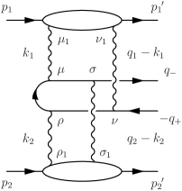
Fig. 1: Typical Feynman diagram for the amplitude $M_{(2)}^{(2)}$

Let us consider the creation of the lepton pair by four virtual photons (Fig. 1). The photons with momenta $k_{1}$, $q_{1}-k_{1}$ (in the latter article, referred to as photons $1$ and $2$) are emitted by the ion A and the photons with momenta $k_{2}$, $q_{2}-k_{2}$ (referred as the photons $3$ and $4$) by the ion B. The main contribution to the cross section gives the following regions of the Sudakov variables:

$$\alpha_{1}\ll\beta_{1}\sim b_{1},\quad\beta_{+}+\beta_{-}=b_{1},$$

$$\beta_{2}\ll\alpha_{2}\sim a_{2},\quad\alpha_{+}+\alpha_{-}=a_{2},$$ (5)

$$|a_{1}|\ll a_{2},\quad|b_{2}|\ll b_{1},\quad q_{i\bot}=\mbox{\boldmath$q$}_{i},\quad\mbox{\boldmath$q$}_{1}+\mbox{\boldmath$q$}_{2}=\mbox{\boldmath$q$}_{+}+\mbox{\boldmath$q$}_{-},$$

$$\alpha_{\pm}=\frac{\mbox{\boldmath$q$}_{\pm}^{2}}{s\beta_{\pm}},\quad\mbox{\boldmath$q$}_{\pm}^{2}\gg m^{2}.$$

Hereinafter $\mbox{\boldmath$q$}_{i}$ denotes the 2–dimensional transverse part of any considered momenta. For definitness, we suggest $\beta_{+},\>\beta_{-}>0$, which corresponds to the situation when the pair moves along the ion $A$ (the momentum $p_{1}$). Bearing in mind a possible extension to pQCD we neglect the lepton masses whenever appropriate.

The contribution to the matrix element of such a set of Feynman diagrams (FD) reads

$$M^{(2)}_{(2)}=\mathrm{i}s\frac{(Z_{1}Z_{2})^{2}(4\pi\alpha)^{4}}{(2\pi)^{8}}\int\frac{\mathrm{d}^{4}k_{1}\mathrm{d}^{4}k_{2}}{k_{1}^{2}k_{2}^{2}(q_{1}-k_{1})^{2}(q_{2}-k_{2})^{2}}\\ \times\frac{1}{s}\bar{u}^{\eta}(p_{1}^{\prime})O_{1}^{\mu_{1}\nu_{1}}u^{\eta}(p_{1})\bar{u}^{\lambda}(p_{2}^{\prime})O_{2}^{\rho_{1}\sigma_{1}}u^{\lambda}(p_{2})\bar{u}(q_{-})T^{\mu\nu\rho\sigma}v(q_{+})g_{\mu\mu_{1}}g_{\nu\nu_{1}}g_{\rho\rho_{1}}g_{\sigma\sigma_{1}}.$$ (6)

To see the proportionality of the matrix element (6) to invariant energy $s$, we use the Gribov representation for virtual photon Green functions

$$g_{\mu\mu_{1}}g_{\nu\nu_{1}}g_{\rho\rho_{1}}g_{\sigma\sigma_{1}}\approx\Big{(}\frac{2}{s}\Big{)}^{4}p_{1\mu}p_{1\nu}p_{1\rho_{1}}p_{1\sigma_{1}}p_{2\mu_{1}}p_{2\nu_{1}}p_{2\rho}p_{2\sigma}.$$ (7)

Numerators of Green functions of the nuclei $A$ can be written as $s^{2}N_{1}$ with $N_{1}=\bar{u}^{\eta}(p_{1}^{\prime})\hat{p}_{2}u^{\eta}(p_{1})/s$, $\sum\limits_{\eta}|N_{1}|^{2}=2$ and a similar expression takes place for the nuclei $B$. The denominators of virtual photon Green functions in the considered kinematics depend only on transverse components of the corresponding 4-vectors, thus

$$k_{1}^{2}k_{2}^{2}(q_{1}-k_{1})^{2}(q_{2}-k_{2})^{2}=\mbox{\boldmath$k$}_{1}^{2}\mbox{\boldmath$k$}_{2}^{2}(\mbox{\boldmath$q$}_{1}-\mbox{\boldmath$k$}_{1})^{2}(\mbox{\boldmath$q$}_{2}-\mbox{\boldmath$k$}_{2})^{2}.$$

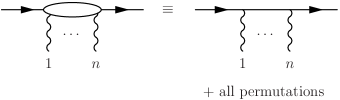
Fig. 2: The notation for the permutations of $n$ virtual photons emitted by the heavy ion.

There are 24 FD contributing to $M^{(2)}_{(2)}$. Instead of them it is convenient to consider $24\ast 2\ast 2=96$ FD which take as well the permutations of emission and absorption points of exchanged photons to the nuclei (Fig. 2). Then the result must be divided by $(2!)^{2}$. This trick Gribov:1970ik provides the convergence of integrals over $\beta_{2}$

$$\frac{1}{2\pi\mathrm{i}}\int\limits_{-\infty}^{\infty}\mathrm{d}\beta_{2}\bigg{[}\frac{s}{s\beta_{2}-c+\mathrm{i}0}+\frac{s}{-s\beta_{2}-d+\mathrm{i}0}\bigg{]}=-1,$$ (8)

and a similar integral over the variable $\alpha_{1}$. After all operations we can write the matrix element in the form

$$M_{(2)}^{(2)}=\mathrm{i}s\frac{(16\pi\alpha^{2}Z_{1}Z_{2})^{2}N_{1}N_{2}}{(2!)^{2}}\int\frac{\mathrm{d}^{2}\mbox{\boldmath$k$}_{1}\mathrm{d}^{2}\mbox{\boldmath$k$}_{2}}{\pi^{2}}\frac{\bar{u}(q_{-})Rv(q_{+})}{\mbox{\boldmath$k$}_{1}^{2}\mbox{\boldmath$k$}_{2}^{2}(\mbox{\boldmath$q$}_{1}-\mbox{\boldmath$k$}_{1})^{2}(\mbox{\boldmath$q$}_{2}-\mbox{\boldmath$k$}_{2})^{2}},$$ (9)

with

$$R=\frac{1}{s}\int\frac{\mathrm{d}\beta_{1}\mathrm{d}\alpha_{2}}{(2\pi\mathrm{i})^{2}}p_{1\mu}p_{1\nu}p_{2\rho}p_{2\sigma}T^{\mu\nu\rho\sigma}.$$

II.2 The classification of diagrams

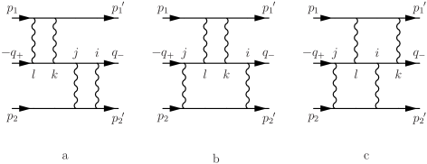
Fig. 3: The set of basic Feynman diagrams for the amplitude $M_{(2)}^{(2)}$.

It is convenient to classify FD by order of exchanged photons absorbed by the lepton world line (Fig. 3). We mark them as $R_{ijkl}$, $R=\sum R_{ijkl}$ with different integers $i,j,k,l$ from one to four, counting from a negative lepton emission point.

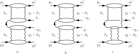
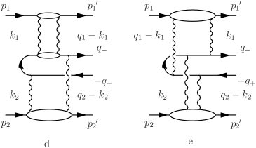
Fig. 4: The Feynman diagrams for the amplitude $M_{(2)}^{(2)}$.

a) Consider first the set of 4 FD (Fig. 4a) named $R_{1234}$, $R_{2134}$, $R_{1243}$, $R_{2143}$ in which the interactions with two nuclei are ordered consecutively against the lepton line direction. The sum of relevant contributions provides the convergence of $\beta_{1},\alpha_{2}$ integrations. After a standard calculation one obtains for this set

$$R_{1234}+R_{2134}+R_{1243}+R_{2143}=\frac{\beta_{-}\hat{p}_{1}(\hat{q}_{-}-\hat{q}_{1})_{\bot}}{\beta_{+}\mbox{\boldmath$q$}_{-}^{2}+\beta_{-}(\mbox{\boldmath$q$}_{-}-\mbox{\boldmath$q$}_{1})^{2}}\frac{\hat{p}_{2}}{s}=-B\frac{\hat{p}_{2}}{s},$$

$$B=\frac{\hat{q}_{-\bot}(\hat{q}_{-}-\hat{q}_{1})_{\bot}}{\beta_{+}\mbox{\boldmath$q$}_{-}^{2}+\beta_{-}(\mbox{\boldmath$q$}_{-}-\mbox{\boldmath$q$}_{1})^{2}}.$$ (10)

The last equality in (10) is the result of Dirac equation for massless particles

$$\bar{u}(q_{-})\beta_{-}\hat{p}_{1}\hat{p}_{2}=-\bar{u}(q_{-})\hat{q}_{-\bot}\hat{p}_{2}.$$ (11)

A similar result as in (10) is achieved for the set of crossing diagrams (Fig. 4b) relevant to $R_{3412}$, $R_{3421}$, $R_{4312}$, $R_{4321}$ terms in the amplitude with only the replacement $B\to\tilde{B}$ where for $\tilde{B}$ stands

$$\tilde{B}=\frac{(-\hat{q}_{+}+\hat{q}_{1})_{\bot}\hat{q}_{+\bot}}{\beta_{-}\mbox{\boldmath$q$}_{+}^{2}+\beta_{+}(\mbox{\boldmath$q$}_{1}-\mbox{\boldmath$q$}_{+})^{2}}.$$ (12)

b) Let us now consider the set of the diagrams $R_{1342}$, $R_{1432}$, $R_{2341}$, $R_{2431}$(Fig. 4c) and $R_{3124}$, $R_{3214}$, $R_{4123}$, $R_{4213}$ (Fig. 4d), where exchanges with the ion B(A) are attached to the lepton line between the interaction with the ion A(B).

For definiteness, consider the sum $R_{1342}+R_{1432}$. Using the relevant denominators of the lepton line one obtains the following integrals over $\beta_{1}$, $\alpha_{2}$:

$$\int\frac{\mathrm{d}\beta_{1}}{2\pi\mathrm{i}}\frac{1}{s\alpha_{-}(\beta_{-}-\beta_{1})-(\mbox{\boldmath$q$}_{-}-\mbox{\boldmath$k$}_{1})^{2}+\mathrm{i}0}$$

$$\times\frac{1}{-s\alpha_{+}(\beta_{-}-\beta_{1})-(-\mbox{\boldmath$q$}_{+}+\mbox{\boldmath$q$}_{1}-\mbox{\boldmath$k$}_{1})^{2}+\mathrm{i}0}$$

$$\times\int\frac{\mathrm{d}\alpha_{2}}{2\pi\mathrm{i}}\Big{[}\frac{s(\beta_{-}-\beta_{1})}{s(\beta_{-}-\beta_{1})(\alpha_{-}-\alpha_{2})-(\mbox{\boldmath$q$}_{-}-\mbox{\boldmath$k$}_{1})^{2}+\mathrm{i}0}$$

$$+\frac{s(\beta_{-}-\beta_{1})}{s(\beta_{-}-\beta_{1})(-\alpha_{+}+\alpha_{2})-(-\mbox{\boldmath$q$}_{+}+\mbox{\boldmath$q$}_{1}-\mbox{\boldmath$k$}_{1})^{2}+\mathrm{i}0}\Big{]}.$$ (13)

The second integral after closing the integration contour in the lower half plane gives the function $\operatorname{sgn}(\beta_{-}-\beta_{1})$, thus (II.2) becomes

$$\int\frac{\mathrm{d}\beta_{1}}{2\pi\mathrm{i}}\,\frac{\operatorname{sgn}(\beta_{1}-\beta_{-})}{s\alpha_{-}(\beta_{-}-\beta_{1})-(\mbox{\boldmath$q$}_{-}-\mbox{\boldmath$k$}_{1})^{2}+\mathrm{i}0}$$

$$\times\frac{1}{(-s\alpha_{+}(\beta_{-}-\beta_{1})-(-\mbox{\boldmath$q$}_{+}+\mbox{\boldmath$q$}_{1}-\mbox{\boldmath$k$}_{1})^{2}+\mathrm{i}0)}.$$ (14)

Using the relation

$$\int\limits_{-\infty}^{\infty}\frac{\mathrm{d}x}{2\pi\mathrm{i}}\frac{\operatorname{sgn}(x)}{(-ax-b+\mathrm{i}0)(cx-d+\mathrm{i}0)}=\frac{1}{\pi\mathrm{i}(ad+bc)}\ln\frac{ad}{bc},$$ (15)

we obtained the following result:

$$R_{1342} +R_{1432}+R_{2341}+R_{2431}=$$

$$\frac{\hat{p}_{1}}{\mathrm{i}\pi s}\bigg{(}\frac{(\hat{q}_{-}-\hat{k}_{1})_{\bot}(-\hat{q}_{+}+\hat{q}_{1}-\hat{k}_{1})_{\bot}}{\alpha_{+}(\mbox{\boldmath$q$}_{-}-\mbox{\boldmath$k$}_{1})^{2}+\alpha_{-}(-\mbox{\boldmath$q$}_{+}+\mbox{\boldmath$q$}_{1}-\mbox{\boldmath$k$}_{1})^{2}}\ln\frac{\alpha_{+}(\mbox{\boldmath$q$}_{-}-\mbox{\boldmath$k$}_{1})^{2}}{\alpha_{-}(-\mbox{\boldmath$q$}_{+}+\mbox{\boldmath$q$}_{1}-\mbox{\boldmath$k$}_{1})^{2}}$$

$$\quad+ \frac{(\hat{q}_{-}-\hat{q}_{1}+\hat{k}_{1})_{\bot}(-\hat{q}_{+}+\hat{k}_{1})_{\bot}}{\alpha_{+}(\mbox{\boldmath$q$}_{-}-\mbox{\boldmath$q$}_{1}+\mbox{\boldmath$k$}_{1})^{2}+\alpha_{-}(-\mbox{\boldmath$q$}_{+}+\mbox{\boldmath$k$}_{1})^{2}}\ln\frac{\alpha_{+}(\mbox{\boldmath$q$}_{-}-\mbox{\boldmath$q$}_{1}+\mbox{\boldmath$k$}_{1})^{2}}{\alpha_{-}(-\mbox{\boldmath$q$}_{+}+\mbox{\boldmath$k$}_{1})^{2}}\bigg{)},$$ (16a)

$$R_{3124} +R_{3214}+R_{4123}+R_{4213}=$$

$$\frac{\hat{p}_{2}}{\mathrm{i}\pi s}\bigg{(}\frac{(\hat{q}_{-}-\hat{k}_{2})_{\bot}(-\hat{q}_{+}+\hat{q}_{2}-\hat{k}_{2})_{\bot}}{\beta_{+}(\mbox{\boldmath$q$}_{-}-\mbox{\boldmath$k$}_{2})^{2}+\beta_{-}(-\mbox{\boldmath$q$}_{+}+\mbox{\boldmath$q$}_{2}-\mbox{\boldmath$k$}_{2})^{2}}\ln\frac{\beta_{-}(-\mbox{\boldmath$q$}_{+}+\mbox{\boldmath$q$}_{2}-\mbox{\boldmath$k$}_{2})^{2}}{\beta_{+}(\mbox{\boldmath$q$}_{-}-\mbox{\boldmath$k$}_{2})^{2}}$$

$$\quad+ \frac{(\hat{q}_{-}-\hat{q}_{2}+\hat{k}_{2})_{\bot}(-\hat{q}_{+}+\hat{k}_{2})_{\bot}}{\beta_{+}(\mbox{\boldmath$q$}_{-}-\mbox{\boldmath$q$}_{2}+\mbox{\boldmath$k$}_{2})^{2}+\beta_{-}(-\mbox{\boldmath$q$}_{+}+\mbox{\boldmath$k$}_{2})^{2}}\ln\frac{\beta_{-}(-\mbox{\boldmath$q$}_{+}+\mbox{\boldmath$k$}_{2})^{2}}{\beta_{+}(\mbox{\boldmath$q$}_{-}-\mbox{\boldmath$q$}_{2}+\mbox{\boldmath$k$}_{2})^{2}}\bigg{)}.$$ (16b)

It is necessary to point out that the obtained expressions (16-16) are pure imaginary and consequently their interference with the Born term in the cross section is zero.

c) Consider the case of interactions with different nuclei alternating along the lepton line, for instance, the amplitude $R_{1324}$ (Fig. 4e). After a bit algebra one obtains for the relevant numerator

$$N_{1324}=s\hat{p}_{1}\hat{p}_{2}(\hat{q}_{-}-\hat{k}_{1})_{\bot}(\hat{q}_{-}-\hat{k}_{1}-\hat{k}_{2})_{\bot}(\hat{q}_{-}-\hat{q}_{1}-\hat{k}_{2})_{\bot},$$ (17)

which is very different from the numerators of the Born like amplitudes. Specifically, it is the term of higher order in the running transverse momenta $\mbox{\boldmath$k$}_{i}$.

The relevant denominators read

$$\{1\} =(q_{-}-k_{1})^{2}+i0=s(\beta_{-}-\beta_{1})\alpha_{-}-(\mbox{\boldmath$q$}_{-}-\mbox{\boldmath$k$}_{1})^{2}+i0,$$ (18)

$$\{2\} =(q_{-}-k_{1}-k_{2})^{2}+\mathrm{i}0=s(\beta_{-}-\beta_{1})(\alpha_{-}-\alpha_{2})-(\mbox{\boldmath$q$}_{-}-\mbox{\boldmath$k$}_{1}-\mbox{\boldmath$k$}_{2})^{2}+\mathrm{i}0,$$

$$\{3\} =(-q_{+}+q_{2}-k_{2})^{2}+\mathrm{i}0=s(-\beta_{+})(\alpha_{-}-\alpha_{2})-(-\mbox{\boldmath$q$}_{+}+\mbox{\boldmath$q$}_{2}-\mbox{\boldmath$k$}_{2})^{2}+\mathrm{i}0.$$

The nonvanishing contribution only emerges if the poles are located in different $\alpha_{2}$ half–planes, which takes place only if $\beta_{1}<\beta_{-}$ ($\beta_{\pm}>0$). Taking the residue at the pole {2} we find

$$\int\frac{s\mathrm{d}\alpha_{2}}{2\pi\mathrm{i}}\frac{1}{\{2\}\{3\}}=-\frac{\theta(\beta_{-}-\beta_{1})}{(\beta_{1}-\beta_{-})(-\mbox{\boldmath$q$}_{+}+\mbox{\boldmath$q$}_{2}-\mbox{\boldmath$k$}_{2})^{2}-\beta_{+}(\mbox{\boldmath$q$}_{-}-\mbox{\boldmath$k$}_{1}-\mbox{\boldmath$k$}_{2})^{2}}.$$ (19)

Further integration over $\beta_{1}$ can be done using the relation

$$\int\limits_{-\infty}^{\infty}\frac{\mathrm{d}x}{2\pi\mathrm{i}}\frac{\theta(x)}{(ax-b+\mathrm{i}0)(cx+d+\mathrm{i}0)}=\frac{-1}{2(ad+bc)}\left(1+\frac{\mathrm{i}}{\pi}\ln\frac{ad}{bc}\right),$$ (20)

wit the result

$$R_{1324}=-\frac{\beta_{-}N_{1324}}{2sD_{1324}}\left(1+\frac{\mathrm{i}}{\pi}\ln\frac{ad}{bc}\right),$$

$$D_{1324}=\beta_{-}(\mbox{\boldmath$q$}_{-}-\mbox{\boldmath$k$}_{1})^{2}(-\mbox{\boldmath$q$}_{+}+\mbox{\boldmath$q$}_{2}-\mbox{\boldmath$k$}_{2})^{2}+\beta_{+}\mbox{\boldmath$q$}_{-}^{2}(\mbox{\boldmath$q$}_{-}-\mbox{\boldmath$k$}_{1}-\mbox{\boldmath$k$}_{2})^{2}=ad+bc.$$ (21)

The highly nonlinear denominator (21) makes the contribution from the considered case dramatically different from the Born like amplitude. Technically, the nonlinearity is not surprising because of the related nonlinearity of the numerator. The principal difference from the Born like amplitude is that with the alternating ordering of interactions we have the situation in which the $p_{+}$ component of the lightcone momentum is conserved in the scattering on one ion but is not conserved in the scattering on the second ion. Depending on the ordering of interaction vertices and the order of integrations one will encounter the mismatch of conservation and nonconservation of the $p_{-}$ component of the lightcone momentum.

Similar results can be obtained for other contributions of these types.

d) The final result reads

$$M^{(2)}_{(2)}=\frac{\mathrm{i}s}{(2!)^{2}}(16\pi\alpha^{2}Z_{1}Z_{2})^{2}N_{1}N_{2}\int\frac{\mathrm{d}^{2}\mbox{\boldmath$k$}_{1}}{\pi}\frac{\mathrm{d}^{2}\mbox{\boldmath$k$}_{2}}{\pi}\frac{\bar{u}(q_{-})R^{(2)}_{(2)}\frac{\hat{p}_{2}}{s}v(q_{+})}{\mbox{\boldmath$k$}_{1}^{2}\mbox{\boldmath$k$}_{2}^{2}(\mbox{\boldmath$q$}_{1}-\mbox{\boldmath$k$}_{1})^{2}(\mbox{\boldmath$q$}_{2}-\mbox{\boldmath$k$}_{2})^{2}},$$ (22)

$$R_{(2)}^{(2)}= \phantom{+}\sum_{n=1}^{2}\frac{[\hat{a}_{n}\hat{b}_{n}]_{\bot}}{\beta_{-}\mbox{\boldmath$b$}_{n}^{2}+\beta_{+}\mbox{\boldmath$a$}_{n}^{2}}$$

$$-\sum_{n=3}^{10}\frac{[\hat{a}_{n}\hat{b}_{n}\hat{c}_{n}\hat{d}_{n}]_{\bot}}{2[\beta_{-}\mbox{\boldmath$b$}_{n}^{2}\mbox{\boldmath$d$}_{n}^{2}+\beta_{+}\mbox{\boldmath$a$}_{n}^{2}\mbox{\boldmath$c$}_{n}^{2}]}\bigg{(}1+\mathrm{i}\frac{(-1)^{n+1}}{\pi}\ln\frac{\beta_{-}\mbox{\boldmath$b$}_{n}^{2}\mbox{\boldmath$d$}_{n}^{2}}{\beta_{+}\mbox{\boldmath$a$}_{n}^{2}\mbox{\boldmath$c$}_{n}^{2}}\bigg{)}$$

$$+\sum_{n=11}^{12}\mathrm{i}\frac{(-1)^{n+1}}{\pi}\frac{[\hat{a}_{n}\hat{b}_{n}]_{\bot}}{\beta_{-}\mbox{\boldmath$b$}_{n}^{2}+\beta_{+}\mbox{\boldmath$a$}_{n}^{2}}\ln\frac{\beta_{-}\mbox{\boldmath$b$}_{n}^{2}}{\beta_{+}\mbox{\boldmath$a$}_{n}^{2}}.$$ (23)

n	$R_{ijkl}$	$a_{n}$	$b_{n}$	$c_{n}$	$d_{n}$
1	$R_{(12)(34)}$	$q_{-}$	$q_{-}-q_{1}$	—	—
2	$R_{(34)(12)}$	$q_{1}-q_{+}$	$q_{+}$	—	—
3	$R_{1324}$	$q_{-}$	$q_{-}-k_{1}$	$q_{-}-k_{1}-k_{2}$	$q_{-}-q_{1}-k_{2}$
4	$R_{1423}$	$q_{-}$	$q_{-}-k_{1}$	$q_{-}-q_{2}+k_{2}-k_{1}$	$-q_{+}+k_{2}$
5	$R_{2314}$	$q_{-}$	$q_{-}-q_{1}+k_{1}$	$q_{-}-q_{1}+k_{1}-k_{2}$	$-q_{+}+q_{2}-k_{2}$
6	$R_{2413}$	$q_{-}$	$q_{-}-q_{1}+k_{1}$	$-q_{+}+k_{1}+k_{2}$	$-q_{+}+k_{2}$
7	$R_{4231}$	$q_{-}-q_{2}+k_{2}$	$-q_{+}+k_{1}+k_{2}$	$-q_{+}+k_{1}$	$q_{+}$
8	$R_{3241}$	$q_{-}-k_{2}$	$q_{-}-q_{1}+k_{1}-k_{2}$	$-q_{+}+k_{1}$	$q_{+}$
9	$R_{4132}$	$q_{-}-q_{2}+k_{2}$	$q_{-}-q_{2}+k_{2}-k_{1}$	$-q_{+}+q_{1}-k_{1}$	$q_{+}$
10	$R_{3142}$	$q_{-}-k_{2}$	$q_{-}-k_{1}-k_{2}$	$-q_{+}+q_{1}-k_{1}$	$q_{+}$
11	$R_{3(12)4}$	$q_{-}-k_{2}$	$-q_{+}+q_{2}-k_{2}$	—	—
12	$R_{4(12)3}$	$q_{-}-q_{2}+k_{2}$	$-q_{+}+k_{2}$	—	—

Tab. 1: The coefficients for formula (II.2). The brackets denote index permutation, e. g., $(12)\equiv 12+21$.

To convince the gauge invariance fulfilment we put the explicit form for the real part of the amplitude

$$\,\textmd{Re}\,R^{(2)}_{(2)}= \phantom{+}\frac{[\hat{q}_{-}(\hat{q}_{-}-\hat{q}_{1})]_{\bot}}{\beta_{+}\mbox{\boldmath$q$}_{-}^{2}+\beta_{-}(\mbox{\boldmath$q$}_{-}-\mbox{\boldmath$q$}_{1})^{2}}+\frac{[(-\hat{q}_{+}+\hat{q}_{1})\hat{q}_{+}]_{\bot}}{\beta_{-}\mbox{\boldmath$q$}_{+}^{2}+\beta_{+}(\mbox{\boldmath$q$}_{+}-\mbox{\boldmath$q$}_{1})^{2}}$$

$$\phantom{+}\frac{[\hat{q}_{-}(\hat{q}_{-}-\hat{k}_{1})(\hat{q}_{-}-\hat{k}_{1}-\hat{k}_{2})(\hat{q}_{-}-\hat{q}_{1}-\hat{k}_{2})]_{\bot}}{2[\beta_{-}(\mbox{\boldmath$q$}_{-}-\mbox{\boldmath$k$}_{1})^{2}(-\mbox{\boldmath$q$}_{+}+\mbox{\boldmath$q$}_{2}-\mbox{\boldmath$k$}_{2})^{2}+\beta_{+}\mbox{\boldmath$q$}_{-}^{2}(\mbox{\boldmath$q$}_{-}-\mbox{\boldmath$k$}_{1}-\mbox{\boldmath$k$}_{2})^{2}]}$$

$$-\frac{[\hat{q}_{-}(\hat{q}_{-}-\hat{k}_{1})(\hat{q}_{-}-\hat{q}_{2}+\hat{k}_{2}-\hat{k}_{1})(-\hat{q}_{+}+\hat{k}_{2})]_{\bot}}{2[\beta_{-}(\mbox{\boldmath$q$}_{-}-\mbox{\boldmath$k$}_{1})^{2}(-\mbox{\boldmath$q$}_{+}+\mbox{\boldmath$k$}_{2})^{2}+\beta_{+}\mbox{\boldmath$q$}_{-}^{2}(\mbox{\boldmath$q$}_{-}-\mbox{\boldmath$q$}_{2}+\mbox{\boldmath$k$}_{2}-\mbox{\boldmath$k$}_{1})^{2}]}$$

$$-\frac{[\hat{q}_{-}(\hat{q}_{-}-\hat{q}_{1}+\hat{k}_{1})(\hat{q}_{-}-\hat{q}_{1}+\hat{k}_{1}-\hat{k}_{2})(-\hat{q}_{+}+\hat{q}_{2}-\hat{k}_{2})]_{\bot}}{2[\beta_{-}(\mbox{\boldmath$q$}_{-}-\mbox{\boldmath$q$}_{1}+\mbox{\boldmath$k$}_{1})^{2}(-\mbox{\boldmath$q$}_{+}+\mbox{\boldmath$q$}_{2}-\mbox{\boldmath$k$}_{2})^{2}+\beta_{+}\mbox{\boldmath$q$}_{-}^{2}(\mbox{\boldmath$q$}_{-}-\mbox{\boldmath$q$}_{1}+\mbox{\boldmath$k$}_{1}-\mbox{\boldmath$k$}_{2})^{2}]}$$

$$-\frac{[\hat{q}_{-}(\hat{q}_{-}-\hat{q}_{1}+\hat{k}_{1})(-\hat{q}_{+}+\hat{k}_{1}+\hat{k}_{2})(-\hat{q}_{+}+\hat{k}_{2})]_{\bot}}{2[\beta_{-}(\mbox{\boldmath$q$}_{-}-\mbox{\boldmath$q$}_{1}+\mbox{\boldmath$k$}_{1})^{2}(-\mbox{\boldmath$q$}_{+}+\mbox{\boldmath$k$}_{2})^{2}+\beta_{+}\mbox{\boldmath$q$}_{-}^{2}(-\mbox{\boldmath$q$}_{+}+\mbox{\boldmath$k$}_{1}+\mbox{\boldmath$k$}_{2})^{2}]}$$

$$-\frac{[(\hat{q}_{-}-\hat{q}_{2}+\hat{k}_{2})(-\hat{q}_{+}+\hat{k}_{1}+\hat{k}_{2})(-\hat{q}_{+}+\hat{k}_{1})\hat{q}_{+}]_{\bot}}{2[\beta_{-}\mbox{\boldmath$q$}_{+}^{2}(-\mbox{\boldmath$q$}_{+}+\mbox{\boldmath$k$}_{1}+\mbox{\boldmath$k$}_{2})^{2}+\beta_{+}(-\mbox{\boldmath$q$}_{+}+\mbox{\boldmath$k$}_{1})^{2}(\mbox{\boldmath$q$}_{-}-\mbox{\boldmath$q$}_{2}+\mbox{\boldmath$k$}_{2})^{2}]}$$

$$-\frac{[(\hat{q}_{-}-\hat{k}_{2})(\hat{q}_{-}-\hat{q}_{1}+\hat{k}_{1}-\hat{k}_{2})(-\hat{q}_{+}+\hat{k}_{1})\hat{q}_{+}]_{\bot}}{2[\beta_{-}\mbox{\boldmath$q$}_{+}^{2}(\mbox{\boldmath$q$}_{-}-\mbox{\boldmath$q$}_{1}+\mbox{\boldmath$k$}_{1}-\mbox{\boldmath$k$}_{2})^{2}+\beta_{+}(-\mbox{\boldmath$q$}_{+}+\mbox{\boldmath$k$}_{1})^{2}(\mbox{\boldmath$q$}_{-}-\mbox{\boldmath$k$}_{2})^{2}]}$$

$$-\frac{[(\hat{q}_{-}-\hat{q}_{2}+\hat{k}_{2})(\hat{q}_{-}-\hat{q}_{2}+\hat{k}_{2}-\hat{k}_{1})(-\hat{q}_{+}+\hat{q}_{1}-\hat{k}_{1})\hat{q}_{+}]_{\bot}}{2[\beta_{-}\mbox{\boldmath$q$}_{+}^{2}(\mbox{\boldmath$q$}_{-}-\mbox{\boldmath$q$}_{2}+\mbox{\boldmath$k$}_{2}-\mbox{\boldmath$k$}_{1})^{2}+\beta_{+}(\mbox{\boldmath$q$}_{-}-\mbox{\boldmath$q$}_{2}+\mbox{\boldmath$k$}_{2})^{2}(-\mbox{\boldmath$q$}_{+}+\mbox{\boldmath$q$}_{1}-\mbox{\boldmath$k$}_{1})^{2}]}$$

$$-\frac{[(\hat{q}_{-}-\hat{k}_{2})(\hat{q}_{-}-\hat{k}_{1}-\hat{k}_{2})(-\hat{q}_{+}+\hat{q}_{1}-\hat{k}_{1})\hat{q}_{+}]_{\bot}}{2[\beta_{-}\mbox{\boldmath$q$}_{+}^{2}(\mbox{\boldmath$q$}_{-}-\mbox{\boldmath$k$}_{1}-\mbox{\boldmath$k$}_{2})^{2}+\beta_{+}(-\mbox{\boldmath$q$}_{+}+\mbox{\boldmath$q$}_{1}-\mbox{\boldmath$k$}_{1})^{2}(\mbox{\boldmath$q$}_{-}-\mbox{\boldmath$k$}_{2})^{2}]}.$$

Then one can verify that the following condition is satisfied:

$$\,\textmd{Re}\,R^{(2)}_{(2)}=0\quad\mathrm{if}\quad\mbox{\boldmath$k$}_{1}=0\quad\mathrm{or}\quad\mbox{\boldmath$k$}_{2}=0\quad\mathrm{or}\quad\mbox{\boldmath$k$}_{1}=\mbox{\boldmath$q$}_{1}\quad\mathrm{or}\quad\mbox{\boldmath$k$}_{2}=\mbox{\boldmath$q$}_{2}.$$ (24)

This fact is correct also for the whole amplitude (II.2). As one can see, this property is crucial for the infrared convergence in integrations over $\mathrm{d}^{2}\mbox{\boldmath$k$}_{i}$ .

Under the loop integration one can make the shift of the integration variable $\mbox{\boldmath$k$}_{i}\to\mbox{\boldmath$q$}_{i}-\mbox{\boldmath$k$}_{i}$. Then expression (II.2) for $\,\textmd{Re}\,R^{(2)}_{(2)}$ can be simplified to

$$\,\textmd{Re}\,R^{(2)}_{(2)}= \phantom{+}\frac{\hat{q}_{-\bot}(\hat{q}_{-}-\hat{q}_{1})_{\bot}}{\beta_{+}\mbox{\boldmath$q$}_{-}^{2}+\beta_{-}(\mbox{\boldmath$q$}_{-}-\mbox{\boldmath$q$}_{1})^{2}}+\frac{(-\hat{q}_{+}+\hat{q}_{1})_{\bot}\hat{q}_{+\bot}}{\beta_{-}\mbox{\boldmath$q$}_{+}^{2}+\beta_{+}(\mbox{\boldmath$q$}_{1}-\mbox{\boldmath$q$}_{+})^{2}}$$

$$-2\frac{[\hat{q}_{-}(\hat{q}_{-}-\hat{k}_{1})(\hat{q}_{-}-\hat{k}_{1}-\hat{k}_{2})(\hat{q}_{-}-\hat{q}_{1}-\hat{k}_{2})]_{\bot}}{\beta_{-}(\mbox{\boldmath$q$}_{-}-\mbox{\boldmath$k$}_{1})^{2}(-\mbox{\boldmath$q$}_{+}+\mbox{\boldmath$q$}_{2}-\mbox{\boldmath$k$}_{2})^{2}+\beta_{+}\mbox{\boldmath$q$}_{-}^{2}(\mbox{\boldmath$q$}_{-}-\mbox{\boldmath$k$}_{1}-\mbox{\boldmath$k$}_{2})^{2}}$$

$$-2\frac{[(-\hat{q}_{+}+\hat{q}_{1}+\hat{k}_{2})(-\hat{q}_{+}+\hat{k}_{1}+\hat{k}_{2})(-\hat{q}_{+}+\hat{k}_{1})\hat{q}_{+}]_{\bot}}{\beta_{-}\mbox{\boldmath$q$}_{+}^{2}(-\mbox{\boldmath$q$}_{+}+\mbox{\boldmath$k$}_{1}+\mbox{\boldmath$k$}_{2})^{2}+\beta_{+}(-\mbox{\boldmath$q$}_{+}+\mbox{\boldmath$k$}_{1})^{2}(\mbox{\boldmath$q$}_{-}-\mbox{\boldmath$q$}_{2}+\mbox{\boldmath$k$}_{2})^{2}}.$$ (25)

Despite the gauge invariance property is not seen clearly her,e as in the previous case, the final results after integration over $k_{i}$ coincide.

III The wide angle limit of the $M^{(2)}_{(2)}$ amplitude

Let us consider the behavior of this expression in the case when the transverse component of lepton momenta is large compared to the momenta transferred to the ions

$$\mbox{\boldmath$q$}_{-}\approx-\mbox{\boldmath$q$}_{+}=\mbox{\boldmath$q$},\quad|\mbox{\boldmath$q$}|\gg|\mbox{\boldmath$q$}_{1,2}|.$$ (26)

In this case, the main contribution to the matrix element gives the region

$$|\mbox{\boldmath$q$}_{i}|\ll|\mbox{\boldmath$k$}_{i}|\ll|\mbox{\boldmath$q$}|.$$ (27)

The amplitude $M^{(1)}_{(1)}$ reads

$$M^{(1)}_{(1)}=-\mathrm{i}s\frac{(8\pi\alpha)^{2}N_{1}N_{2}Z_{1}Z_{2}}{\mbox{\boldmath$q$}_{1}^{2}\mbox{\boldmath$q$}_{2}^{2}}\bar{u}(q_{-})\frac{R^{(1)}_{(1)}}{s}v(q_{+}),$$ (28)

$$R^{(1)}_{(1)}=\frac{1}{s}\hat{p}_{1}\frac{\hat{q}_{-}-\hat{q}_{1}}{(q_{-}-q_{1})^{2}}\hat{p}_{2}+\hat{p}_{2}\frac{\hat{q}_{1}-\hat{q}_{+}}{(q_{1}-q_{+})^{2}}\hat{p}_{1}=(B-\tilde{B})\hat{p}_{2}.$$

For wide angle kinematics one has

$$\frac{1}{s}R^{(1)}_{(1)}=\frac{\hat{p}_{2}}{s}\frac{1}{b_{1}^{2}(\mbox{\boldmath$q$}^{2})^{2}}[2\mbox{\boldmath$q$}.\mbox{\boldmath$q$}_{2}[b_{1}\hat{q}\hat{q}_{1}+2\beta_{-}\mbox{\boldmath$q$}.\mbox{\boldmath$q$}_{1}]+\mbox{\boldmath$q$}^{2}[b_{1}\hat{q}_{1}\hat{q}_{2}+2\beta_{+}\mbox{\boldmath$q$}_{1}.\mbox{\boldmath$q$}_{2}]],$$ (29)

with $b_{1}=\beta_{-}+\beta_{+}$, $\mbox{\boldmath$q$}=\mbox{\boldmath$q$}_{-}\approx-\mbox{\boldmath$q$}_{+}$ and $\mbox{\boldmath$q$}_{1,2}$ are the transferred to ions momenta.

For matrix element $M^{(1)}_{(2)}$ we have (in agreement with the result obtained in paper GPS )

$$M^{(1)}_{(2)}=-s\frac{2^{7}\pi^{2}\alpha^{3}Z_{1}Z_{2}^{2}N_{1}N_{2}}{\mbox{\boldmath$q$}_{1}^{2}}\int\frac{d^{2}\mbox{\boldmath$k$}_{2}}{\pi}\frac{1}{\mbox{\boldmath$k$}_{2}^{2}(\mbox{\boldmath$q$}_{2}-\mbox{\boldmath$k$}_{2})^{2}}\bar{u}(q_{-})R_{(2)}^{(1)}\frac{\hat{p}_{2}}{s}v(q_{+}),$$ (30)

with

$$R_{(2)}^{(1)}=B+\tilde{B}-\frac{(\hat{q}_{-}-\hat{k}_{2})_{\bot}(\hat{q}_{-}-\hat{q}_{1}-\hat{k}_{2})_{\bot}}{\beta_{-}(\mbox{\boldmath$q$}_{-}-\mbox{\boldmath$q$}_{1}-\mbox{\boldmath$k$}_{2})^{2}+\beta_{+}(\mbox{\boldmath$q$}_{-}-\mbox{\boldmath$k$}_{2})^{2}}-\frac{(\hat{q}_{+}-\hat{k}_{2}-\hat{q}_{1})_{\bot}(\hat{q}_{+}-\hat{k}_{2})_{\bot}}{\beta_{+}(\mbox{\boldmath$q$}_{-}-\mbox{\boldmath$q$}_{2}+\mbox{\boldmath$k$}_{2})^{2}+\beta_{-}(\mbox{\boldmath$q$}_{+}-\mbox{\boldmath$k$}_{2})^{2}}.$$ (31)

In the considered limit this expression has the form

$$R_{(2)}^{(1)}\sim \frac{1}{b_{1}\mbox{\boldmath$q$}^{2}}\Big{[}(2\beta_{-}\mbox{\boldmath$q$}_{-}.\mbox{\boldmath$q$}_{1}+\hat{q}_{-}\hat{q}_{1})\Big{(}\frac{4(\mbox{\boldmath$q$}_{-}.\mbox{\boldmath$k$}_{2})^{2}}{(\mbox{\boldmath$q$}^{2})^{2}}-\frac{\mbox{\boldmath$k$}_{2}^{2}}{\mbox{\boldmath$q$}^{2}}\Big{)}$$

$$-\frac{2\mbox{\boldmath$q$}_{-}.\mbox{\boldmath$k$}_{2}}{\mbox{\boldmath$q$}^{2}}(\hat{k}_{2}\hat{q}_{1}+2\beta_{-}\mbox{\boldmath$k$}_{2}.\mbox{\boldmath$q$}_{1})]+(\beta_{-}\to\beta_{+}),\quad|\mbox{\boldmath$k$}_{2}|\gg|\mbox{\boldmath$q$}_{2}|.$$ (32)

This expression turns to zero after the angular averaging. It can be shown that the quantity $M^{(1)}_{(3)}$ as well turns to zero in the limit of wide angles pair production and is proportional to $|\mbox{\boldmath$q$}_{2}|/|\mbox{\boldmath$q$}|\ll 1$, which is in agreement with IM .

For the considered above amplitude $M_{(2)}^{(2)}$ (22) the quantity $R^{(2)}_{(2)}$ plays a role of cut-off in the region $|\mbox{\boldmath$k$}_{i}|>|\mbox{\boldmath$q$}|$. From very general arguments it can be cast in the form

$$\,\textmd{Re}\,R^{(2)}_{(2)}\approx\frac{[k_{1}^{\mu}(q_{1}-k_{1})^{\nu}k_{2}^{\alpha}(q_{2}-k_{2})^{\beta}]_{\bot}}{(\mbox{\boldmath$q$}^{2})^{2}}R_{\mu\nu\alpha\beta},$$ (33)

with some dimensionless tensor matrix $R_{\mu\nu\alpha\beta}$ independent of $\mbox{\boldmath$k$}_{i},\mbox{\boldmath$q$}_{i}$. Expanding the expression (II.2) one gets

$$\int\frac{\mathrm{d}^{2}\mbox{\boldmath$k$}_{1}\mathrm{d}^{2}\mbox{\boldmath$k$}_{2}}{\pi^{2}}\frac{\,\textmd{Re}\,R^{(2)}_{(2)}}{\mbox{\boldmath$k$}_{1}^{2}\mbox{\boldmath$k$}_{2}^{2}(\mbox{\boldmath$q$}_{1}-\mbox{\boldmath$k$}_{1})^{2}(\mbox{\boldmath$q$}_{2}-\mbox{\boldmath$k$}_{2})^{2}}\approx\frac{I}{(\mbox{\boldmath$q$}^{2})^{2}}\frac{4(\beta_{+}-\beta_{-})}{(\beta_{-}+\beta_{+})^{2}}\ln\frac{\mbox{\boldmath$q$}_{max}^{2}}{\mbox{\boldmath$q$}_{1}^{2}}\ln\frac{\mbox{\boldmath$q$}_{max}^{2}}{\mbox{\boldmath$q$}_{2}^{2}},$$ (34)

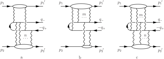
Fig. 5: Some Feynman diagrams for the amplitudes of the type $M^{(2)}_{(n)}$ (a), $M^{(n)}_{(2)}$ (b) and $M^{(m)}_{(n)}$ with $m,n\geq 2$.

where $I$ is the unit matrix and $q_{max}$ is the upper integration limit $q_{max}\simeq 1/R$, $R$ is the nucleus radius. Such enhancement is absent if the number of exchanged photons from every ion exceeds two (Fig. 5). Really, the amplitudes $M^{(2)}_{(n)}$, $M^{(n)}_{(2)}$, $n>2$ contain only the first power of large logarithm, whereas $M^{(m)}_{(n)}$, $m,n>2$ do not contain such a factor at all, because the corresponding loop momenta integrals are convergent in both infrared and ultraviolet regions and one can safely put $|\mbox{\boldmath$q$}_{1(2)}|=0$ over loop integrations.

Thus, the differential cross section for the considered kinematics is determined by the interference term $(M^{(1)}_{(1)})^{*}M^{(2)}_{(2)}$ which has the form (for comparison we present also the Born term)

$$\frac{\mathrm{d}\sigma_{0}}{\mathrm{d}b_{1}\mathrm{d}x} =\frac{16(Z_{1}Z_{2}\alpha^{2})^{2}}{\pi^{4}}\;\frac{(x^{2}+(1-x)^{2})}{\mbox{\boldmath$q$}_{1}^{2}\mbox{\boldmath$q$}_{2}^{2}(\mbox{\boldmath$q$}^{2})^{2}b_{1}}\>\mathrm{d}^{2}q_{1}\mathrm{d}^{2}q_{2}\mathrm{d}^{2}q,$$ (35)

$$\frac{\mathrm{d}\sigma_{int}}{\mathrm{d}b_{1}\mathrm{d}x} =\frac{16(Z_{1}Z_{2}\alpha^{2})^{3}}{\mbox{\boldmath$q$}_{1}^{2}\mbox{\boldmath$q$}_{2}^{2}\mbox{\boldmath$q$}_{+}^{2}\mbox{\boldmath$q$}_{-}^{2}}\frac{(1-2x)}{b_{1}}\ln\frac{\mbox{\boldmath$q$}_{max}^{2}}{\mbox{\boldmath$q$}_{1}^{2}}\ln\frac{\mbox{\boldmath$q$}_{max}^{2}}{\mbox{\boldmath$q$}_{2}^{2}}\>Q\>\mathrm{d}^{2}q_{1}\mathrm{d}^{2}q_{2}\mathrm{d}^{2}q_{-},$$ (36)

$$\;Q=\frac{\mbox{\boldmath$q$}_{-}.(\mbox{\boldmath$q$}_{1}-\mbox{\boldmath$q$}_{-})}{(1-x)\mbox{\boldmath$q$}_{-}^{2}+x(\mbox{\boldmath$q$}_{-}-\mbox{\boldmath$q$}_{1})^{2}}+\frac{\mbox{\boldmath$q$}_{+}.(\mbox{\boldmath$q$}_{+}-\mbox{\boldmath$q$}_{1})}{x\mbox{\boldmath$q$}_{+}^{2}+(1-x)(\mbox{\boldmath$q$}_{1}-\mbox{\boldmath$q$}_{+})^{2}},$$

$$\;x=\frac{\beta_{-}}{b_{1}},\quad\epsilon<x,\quad b_{1}<1-\epsilon,\quad\epsilon=\frac{4m^{2}x(1-x)}{\mbox{\boldmath$q$}_{\pm}^{2}}.$$

We note that expression (36) is symmetric under simultaneous substitutions $q_{+}\leftrightarrow q_{-}$ and $\beta_{+}\leftrightarrow\beta_{-}$ due to the C-even character of the interference.

Finally, from very straightforward generalization of (33) it can be shown that the set of amplitudes with an odd number of exchanges with one or both nuclei is suppressed in the limit of wide angle production

$$M^{(2m)}_{(2n+1)}\sim O\Big{(}\frac{\mid\mbox{\boldmath$q$}_{1}\mid}{\mid\mbox{\boldmath$q$}\mid}\Big{)},\quad M^{(2m+1)}_{(2n)}\sim O\Big{(}\frac{\mid\mbox{\boldmath$q$}_{2}\mid}{\mid\mbox{\boldmath$q$}\mid}\Big{)},\quad M^{(2m+1)}_{(2n+1)}\sim O\Big{(}\frac{\mid\mbox{\boldmath$q$}_{1}\mid\mid\mbox{\boldmath$q$}_{2}\mid}{\mid\mbox{\boldmath$q$}^{2}\mid}\Big{)}.$$ (37)

IV Multiphoton exchange

Let us generalize the above picture for the case of multiple photon exchanges ($m,n>2$). Using the relation

$$I_{n}=\frac{1}{\pi^{n-1}}\int\frac{\mathrm{d}^{2}\mbox{\boldmath$k$}_{1}\dots\mathrm{d}^{2}\mbox{\boldmath$k$}_{n-1}}{(\mbox{\boldmath$k$}_{1}^{2}+\lambda^{2})\dots(\mbox{\boldmath$k$}_{n-1}^{2}+\lambda^{2})((\mbox{\boldmath$q$}-\mbox{\boldmath$k$}_{1}-\dots-\mbox{\boldmath$k$}_{n-1})^{2}+\lambda^{2})}=\frac{n\ln^{n-1}(\frac{\mbox{\boldmath$q$}^{2}}{\lambda^{2}})}{\mbox{\boldmath$q$}^{2}},$$ (38)

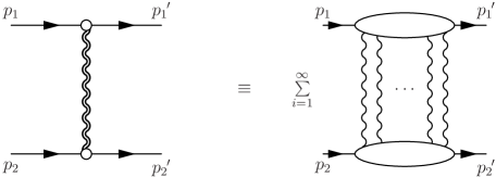
Fig. 6: The representation of all eikonal exchanges.

and taking into account the combinatorial factor $\frac{1}{n!}$ coming from the symmetric integration over $\alpha_{i}$, $\beta_{i}$, one has to replace any single photon exchange by an infinite set of photons, multiplying the amplitude by the factors of type $\exp\{\mathrm{i}\varphi_{i}(\mbox{\boldmath$q$}^{2})\}$ with the phase $\varphi_{i}(\mbox{\boldmath$q$}^{2})=\pm\alpha Z_{i}\ln\frac{\mbox{\boldmath$q$}^{2}}{\lambda}$. The scattering of electron and positron differs only by sign of the phase (positive for electrons) ERG . This replacement is depicted in Fig. 6 where the double photon line corresponds to the infinite set of photons.

Using the same technique as in BGK one can see that the amplitude relevant to Fig. 7a and Fig. 7b can be cast in the form

$$\tilde{R}_{(1)}^{(1)}=B\mathrm{e}^{\displaystyle-\mathrm{i}[\varphi_{1}(\mbox{\boldmath$q$}_{1}^{2})-\varphi_{2}(\mbox{\boldmath$q$}_{2}^{2})]}+\tilde{B}\mathrm{e}^{\displaystyle\mathrm{i}[\varphi_{1}(\mbox{\boldmath$q$}_{1}^{2})-\varphi_{2}(\mbox{\boldmath$q$}_{2}^{2})]}.$$ (39)

The interaction of the electron and the positron with Coulomb field differs only by signs. Though this expression is infrared unstable in the case $Z_{1}\neq Z_{2}$ the regularization parameter $\lambda$ enters it in a standard way.

Let us now consider the class of diagrams depicted on Fig. 7c. In subsection II.2, we obtained the expressions (16, 16) for the case $m=n=2$ such that $\,\textmd{Re}\,R_{1(34)2}=0$. It can be shown that the terms of higher order with any even number of photons from same nuclei attached to the lepton world line between two photons from other nuclei do not contribute to the amplitude of the process under consideration. It is the consequence of the relation $(\operatorname{sgn}(\alpha))^{2k+1}=\operatorname{sgn}(\alpha)$.

The general structure of the amplitude corresponding to Fig. 7c can be constructed using the lowest order truncated amplitude (without single photon propagators) $R_{(2)}^{(1)}$

$$\tilde{R}_{(2)}^{(1)}=\frac{\cos\varphi_{1}(\mbox{\boldmath$q$}_{1}^{2})}{q_{1}^{2}}\bar{R}_{(2)}^{(1)}\mathrm{e}^{\displaystyle\mathrm{i}[\varphi_{2}(\mbox{\boldmath$k$}^{2})-\varphi_{2}((\mbox{\boldmath$q$}_{2}-\mbox{\boldmath$k$})^{2})]},$$

$$\bar{R}_{(2)}^{(1)}=\frac{1}{\mathrm{i}\pi}\frac{(\hat{q}_{-}-\hat{q}_{2}+\hat{k})_{\bot}(-\hat{q}_{+}+\hat{k})_{\bot}}{\beta_{-}(\mbox{\boldmath$q$}_{+}-\mbox{\boldmath$k$})^{2}+\beta_{+}(\mbox{\boldmath$q$}_{-}-\mbox{\boldmath$q$}_{2}+\mbox{\boldmath$k$})^{2}}\ln\frac{\beta_{+}(\mbox{\boldmath$q$}_{-}-\mbox{\boldmath$q$}_{2}+\mbox{\boldmath$k$})^{2}}{\beta_{-}(\mbox{\boldmath$q$}_{+}-\mbox{\boldmath$k$})^{2}}$$ (40)

The further generalization is obvious. For instance, we cite the expression corresponding to the diagram depicted on Fig. 7d

$$\tilde{R}_{(2)}^{(2)}=\cos\varphi_{1}(\mbox{\boldmath$k$}_{1}^{2})\,\mathrm{e}^{\displaystyle-\mathrm{i}\varphi_{1}((\mbox{\boldmath$q$}_{1}-\mbox{\boldmath$k$}_{1})^{2})}\,\cos\varphi_{2}(\mbox{\boldmath$k$}_{2}^{2})\,\mathrm{e}^{\displaystyle\mathrm{i}\varphi_{2}((\mbox{\boldmath$q$}_{2}-\mbox{\boldmath$k$}_{2})^{2})}\,R_{1324}.$$ (41)

From the above consideration we conclude that the general structure of the matrix element $M^{(m)}_{(n)}$, corresponding to $m$ photon exchanges from one ion and $n$ exchanges from other one, schematically reads

$$M^{(m)}_{(n)}=\mathrm{i}sN_{1}N_{2}(Z_{1}\alpha)^{m}(Z_{2}\alpha)^{n}\,\frac{\pi^{2}}{16n!m!}\\ \times\int\frac{\mathrm{d}^{2}k_{1}}{\pi}\cdots\frac{\mathrm{d}^{2}k_{m-1}}{\pi}\,\frac{\mathrm{d}^{2}\kappa_{1}}{\pi}\cdots\frac{\mathrm{d}^{2}\kappa_{n-1}}{\pi}\,\frac{1}{\mbox{\boldmath$k$}^{2}_{1}\dots\mbox{\boldmath$k$}^{2}_{m}}\,\frac{1}{\mbox{\boldmath$\kappa$}_{1}^{2}\dots\mbox{\boldmath$\kappa$}_{n}^{2}}\bar{u}(q_{-})\bar{R}^{(m)}_{(n)}\frac{\hat{p}_{2}}{s}\,v(q_{+}),$$ (42)

where $m$ and $n$ obey the condition $|m-n|\leq 1$. At this stage, we omitted phase factors in the structure ${R}^{(m)}_{(n)}$ (for clearly understanding the problem), so it can be written in the form

$$\bar{R}^{(m)}_{(n)}=\bar{R}^{(1)}_{(1)}+\bar{R}^{(1)}_{(2)}+\bar{R}^{(2)}_{(1)}+\bar{R}^{(2)}_{(2)}+\bar{R}^{(2)}_{(3)}+\bar{R}^{(3)}_{(2)}+\bar{R}^{(3)R}_{(3)}+\bar{R}^{(3)L}_{(3)}\dots$$ (43)

$$\bar{R}^{(2)}_{(1)} =\frac{1}{\mathrm{i}\pi}\frac{(\hat{q}_{-}-\hat{k})_{\bot}(-\hat{q}_{+}+\hat{q}_{1}-\hat{k})_{\bot}}{\alpha_{-}(-\mbox{\boldmath$q$}_{+}+\mbox{\boldmath$q$}_{1}-\mbox{\boldmath$k$})^{2}+\alpha_{+}(\mbox{\boldmath$q$}_{-}-\mbox{\boldmath$k$})^{2}}\ln\frac{\alpha_{+}(\mbox{\boldmath$q$}_{-}-\mbox{\boldmath$k$})^{2}}{\alpha_{-}(-\mbox{\boldmath$q$}_{+}+\mbox{\boldmath$q$}_{1}-\mbox{\boldmath$k$})^{2}},$$

$$\bar{R}^{(2)}_{(3)} =\bar{R}^{(3)}_{(2)}=0,\quad$$

$$\bar{R}^{(3)R}_{(3)} =\frac{1}{c_{1}+c_{2}}\Big{[}3\zeta_{2}+\frac{1}{2}\ln^{2}\frac{c_{1}}{c_{2}}\Big{]},\quad\zeta_{2}=\frac{\pi^{2}}{6},$$

$$c_{1}=\beta_{-}(\mbox{\boldmath$q$}_{-}-\mbox{\boldmath$k$}_{1})^{2}(\mbox{\boldmath$q$}_{-}-\mbox{\boldmath$k$}_{1}-\mbox{\boldmath$k$}_{2}-\mbox{\boldmath$\kappa$}_{1})^{2}(-\mbox{\boldmath$q$}_{+}+\mbox{\boldmath$q$}_{2}-\mbox{\boldmath$\kappa$}_{1}-\mbox{\boldmath$\kappa$}_{2})^{2},$$

$$c_{2}=\beta_{+}\mbox{\boldmath$q$}_{-}^{2}(\mbox{\boldmath$q$}_{-}-\mbox{\boldmath$k$}_{1}-\mbox{\boldmath$\kappa$}_{1})^{2}(\mbox{\boldmath$q$}_{-}-\mbox{\boldmath$k$}_{1}-\mbox{\boldmath$k$}_{2}-\mbox{\boldmath$\kappa$}_{1}-\mbox{\boldmath$\kappa$}_{2})^{2},$$

$$\bar{R}^{(3)}_{(4)} =\frac{1}{d_{1}+d_{2}}\Big{[}3\zeta_{2}+\frac{1}{2}\ln^{2}\frac{d_{1}}{d_{2}}\Big{]}$$

$$d_{1}=\beta_{+}(\mbox{\boldmath$q$}_{-}-\mbox{\boldmath$\kappa$}_{1})^{2}(\mbox{\boldmath$q$}_{-}-\mbox{\boldmath$\kappa$}_{1}-\mbox{\boldmath$\kappa$}_{2}-\mbox{\boldmath$k$}_{1})^{2}(\mbox{\boldmath$q$}_{-}-\mbox{\boldmath$\kappa$}_{1}-\mbox{\boldmath$\kappa$}_{2}-\mbox{\boldmath$\kappa$}_{3}-\mbox{\boldmath$k$}_{1}-\mbox{\boldmath$k$}_{2})^{2},$$

$$d_{2}=\beta_{-}(\mbox{\boldmath$q$}_{-}-\mbox{\boldmath$\kappa$}_{1}-\mbox{\boldmath$k$}_{1})^{2}(\mbox{\boldmath$q$}_{-}-\mbox{\boldmath$\kappa$}_{1}-\mbox{\boldmath$\kappa$}_{2}-\mbox{\boldmath$k$}_{1}-\mbox{\boldmath$k$}_{2})^{2}(-\mbox{\boldmath$q$}_{+}+\mbox{\boldmath$q$}_{2}-\mbox{\boldmath$\kappa$}_{1}-\mbox{\boldmath$\kappa$}_{2}-\mbox{\boldmath$\kappa$}_{3})^{2}.$$ (44)

Here $\bar{R}^{(2)}_{(2)}$ is only the second term in the right–hand side in (II.2) and the index $R(L)$ denotes two possible configurations of photons for $\bar{R}^{(3)R}_{(3)}$ (Fig. 7e) and $\bar{R}^{(3)L}_{(3)}$ (Fig. 7f).

In such a way, the general algorithm for construction of an arbitrary term is transparent. Unfortunately, we cannot obtain the compact expression for the whole amplitude. The reason is the increasing nonlinearity of the propagators with the order of interaction. The behavior of the above denominators is very different from the Born–like case, where the simplicity of propagators allows one to obtain eikonal–like expressions.

V Conclusions

The wide angle lepton pair production in peripheral interactions of ultrarelativistic heavy ions is an archetype reaction for hard processes in central hadronic hard collisions of heavy nuclei. In the electromagnetic case, the expansion parameter $Z_{1,2}\,\alpha\sim 1$ makes the multiple photon collisions, $m\gamma+n\gamma\to\mathrm{l}^{+}\mathrm{l}^{-}$ potentially important ones, likewise the effect of multiple gluon collisions in central collisions is enhanced by a large number of nucleons at the same impact parameter. The crucial issue is whether such multiple photon collisions can be described by the Born cross section in terms of the collective photon fields of colliding nuclei or not. We obtained the expression for the amplitude $2\gamma+2\gamma\to\mathrm{l}^{+}\mathrm{l}^{-}$ and show that its contribution is dominant in a wide angle limit. Our principal finding is that the amplitude is manifestly of non–Born nature, which is suggestive of the complete failure of linear $k_{\perp}$–factorization even in the Abelian case.

We have shown that the terms in perturbation series of the amplitude for the process of lepton pair production in the Coulomb fields of two relativistic nuclei relevant to the closed two photon loops are logarithmically enhanced in this case, while in higher order terms such enhancement is absent. We presented the algorithm which allows one to construct the full amplitude in all orders. The obtained results can be useful in application to the QCD process of production of high $k_{\bot}$ jets, the issue which will be investigated elsewhere.

.

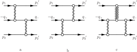
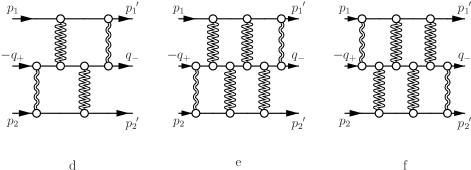
Fig. 7: The Feynman diagrams for the amplitudes with many photon exchanges. The double photon line represents any number of exchanged photons, the double zigzag line represents only the odd number of exchanged photons.

References

• (1) H. Bethe and L. Maximon, Phys. Rev. 93, 768 (1954); H. Davies, H. Bethe and L. Maximon, ibid. 93, 788 (1954)
• (2) L. D. Landau and E. M. Lifshitz, Quantum Mechanics, Nauka, Moscow
• (3) D. Yu. Ivanov and K. Melnikov, Phys. Rev. D57, 4025 (1998)
• (4) S. R. Gevorkyan, S. S. Grigoryan, Phys. Rev. A65, 022505 (2002)
• (5) N. N. Nikolaev, W. Schafer, B. G. Zakharov and V. R. Zoller, JETP Letters 97, 441 (2003)
• (6) N. N. Nikolaev, W. Schafer, B. G. Zakharov and V. R. Zoller (Jülich, Forshungszentrum), 4pp, Aug 2004. Talk given at 12th International Workshop on Deep Inelastic Scattering (DIS 2004), Štrbské Pleso, Slovakia, 14–18 Apr 2004. e-Print Archive: hep-ph/0408054
• (7) A. J. Baltz, L. McLerran, Phys. Rev. C58, (1998)
• (8) B. Segev and J. C. Wells, Phys. Rev. A57, 1849 (1998)
• (9) U. Eichmann, J. Reinhardt and W. Greiner, Phys. Rev. A61, 062710 (2000)
• (10) D. Yu. Ivanov, A. Schiller and V. G. Serbo, Phys. Lett. B457, 155 (1999)
• (11) R. N. Lee and A. I. Milstein, Phys. Rev. A61, 032103 (2000)
• (12) E. Bartoš, S. R. Gevorkyan, N. N. Nikolaev, E. A. Kuraev, Phys. Rev. A66, 042720 (2002)
• (13) E. Bartoš, S. R. Gevorkyan, N. N. Nikolaev, E. A. Kuraev, Phys. Lett. B538, 45 (2002)
• (14) S. R. Gevorkyan and E. A. Kuraev, J. Phys. G: Nucl. Part. Phys. 29, 1227 (2003)
• (15) V. N. Gribov, L. N. Lipatov and G. V. Frolov, Sov. J. Nucl. Phys.  12, 543 (1971) [Yad. Fiz.  12, 994 (1970)].
• (16) E. Bartoš, S. R. Gevorkyan, E. A. Kuraev, Yad. Phys. 67, 8 (2004)
• (17) M. Abramowitz and I. A. Stegun, Handbook of Mathematical Functions, Appl. Math. Ser. No.55, (Washington, DC, 1964)
• (18) I. F. Ginzburg, S. L. Panfil and V. G. Serbo, Nucl. Phys. B284 (1987) 685.
Refer to caption