Abstract

The characteristics of the chiral phase transition are analyzed within the framework of chiral quark models with nonlocal interactions in the mean field approximation. In the chiral limit, we develop a semi-analytic framework which allows us to explicitly determine the phase transition curve, the position of the critical points, some relevant critical exponents, etc. For the case of finite current quark masses, we show the behavior of various thermodynamical and chiral response functions across the phase transition.

PACS numbers: 12.39.Ki,11.30.Rd,12.38.Mh

I Introduction

The behavior of strongly interacting matter under extreme conditions of temperature and/or density has important consequences in nuclear and particle physics as well as in astrophysics and cosmology. From the theoretical point of view, even if a significant progress has been made on the development of ab initio calculations as lattice QCD [1, 2, 3], these are not yet able to provide a detailed knowledge of the full QCD phase diagram, and most theoretical approaches rely in the study of low energy effective models. Qualitatively we expect that chiral symmetry, which is broken at very low temperatures and densities, will be restored as the temperature and/or density are increased. However, the precise characteristics of this phase transition are still not known. For two massless flavors most effective approaches to QCD suggest the existence of a tricritical point on the $(T,\mu)$ plane, which separates a first order phase transition line found at lower $T$ and larger $\mu$, and a second order transition line where the chiral restoration occurs for higher $T$ and lower $\mu$. For two light flavors a similar behavior is expected, although the second order transition line is replaced by a more or less sharp crossover and, correspondingly, the tricritical point becomes an end point. In any case, for a given effective model that can provide a reasonable successful description of low energy strong interactions, it is very important to obtain as much information as possible about the characteristics of the chiral restoration transition. In previous works [4, 5] we have begun the study of chiral restoration in the context of chiral quark models with nonlocal interactions [6], which can be considered as some nonlocal extension of the widely studied Nambu$-$Jona-Lasinio model [7]. In fact, nonlocality arises naturally in the context of several successful approaches to low-energy quark dynamics as, for example, the instanton liquid model [8] and the Schwinger-Dyson resummation techniques [9]. It has been also argued that nonlocal covariant extensions of the NJL model have several advantages over the local scheme like e.g. a natural regularization scheme which automatically preserves the anomalies [10], small NLO corrections [11], etc. In addition, it has been argued [12, 13] that a proper choice of the nonlocal regulator and the model parameters can lead to some form of quark confinement, in the sense that the effective quark propagator has no poles at real energies.

Several studies [13, 14, 15] have shown that these nonlocal chiral quark models provide a satisfactory description of the hadron properties at zero temperature and density. The aim of the present work is to complement the analysis of Refs. [4, 5], presenting further details about the chiral phase transition within these schemes. Indeed, we show that in the chiral limit it is possible to develop a semi-analytic framework which allows us to explicitly determine the phase transition curve, the position of the critical points, some relevant critical exponents, etc. For the case of finite current quark masses, we present the behavior of various thermodynamical and chiral response functions across the phase transition. In particular, it is found that thermal and chiral susceptibilities show clear peaks which allow to define a phase transition temperature as it is usually done in lattice calculations.

The paper is organized as follows. In Sect. II we provide a short description of the model and its treatment in the mean field approximation (MFA). In Sect. III we study the phase transition in the chiral limit by performing the Landau expansion of the free energy. We also obtain the MFA critical exponents. In Sect. IV we present and discuss the behavior of the different thermodynamical and chiral response functions for the case of finite current quark masses, and the corresponding phase diagrams are shown. In Sect. V we present a summary of our main results and conclusions. Finally, some details of the calculations are given in Appendices A and B.

II Nonlocal chiral quark models

Let us begin by stating the Euclidean action for the nonlocal chiral quark model in the case of two light flavors and $SU(2)$ isospin symmetry. One has

$$S_{E}=\int d^{4}x\left[\bar{\psi}(x)\left(-i\hbox to0.0pt{/\hss}\partial+m_{c}\,\leavevmode\hbox{\small 1\kern-3.8pt\normalsize 1}\right)\psi(x)-\frac{G}{2}\,j_{a}(x)j_{a}(x)\right]\ ,$$ (1)

where $\psi=(u\ d)^{T}$ and $m_{c}$ stands for the $u$ and $d$ current quark mass. The current $j_{a}(x)$ is given by

$$j_{a}(x)=\int d^{4}y\ d^{4}z\ \tilde{r}(y-x)\ \tilde{r}(x-z)\ \bar{\psi}(y)\,\Gamma_{a}\,\psi(z)\,,$$ (2)

where $\Gamma_{a}=(\leavevmode\hbox{\small 1\kern-3.8pt\normalsize 1},i\gamma_{5}\vec{\tau})$, and the function $\tilde{r}(x-y)$ is a nonlocal regulator. The latter can be translated into momentum space,

$$\tilde{r}(x-z)=\int\frac{d^{4}p}{(2\pi)^{4}}\ e^{-i(x-z)p}\ r(p)\;.$$ (3)

In fact, dimensional analysis together with Lorentz invariance implies that $r(p)$ can only be a function of $p^{2}/\Lambda^{2}$, where $\Lambda$ is a cutoff parameter describing the range of the nonlocality in momentum space. Hence we will use for the Fourier transform of the regulator the form $r_{\Lambda}(p^{2})$ from now on.

From the Euclidean action in Eq. (1), the partition function for the model at zero $T$ and $\mu$ is defined as

$${\cal Z}_{0}=\int{\cal D}\bar{\psi}{\cal D}\psi\ e^{-S_{E}}\;.$$ (4)

We perform now a standard bosonization of the theory, introducing the sigma and pion meson fields $M_{a}(x)=(\sigma(x),\vec{\pi}(x))$. In this way the partition function can be written as [5]

$${\cal Z}_{0}=\int{\cal D}\sigma{\cal D}\pi\ \det A(M_{a})\ \exp\left[-\frac{1}{2G}\int\frac{d^{4}p}{(2\pi)^{4}}\ M_{a}^{2}(p)\right]\,,$$ (5)

where the operator $A$ reads in momentum space

$$A(M_{a})=(\,-\hbox to0.0pt{/\hss}p+m_{c})\,(2\pi)^{4}\,\delta^{(4)}(p-p^{\prime})+r_{\Lambda}(p^{2})\,M_{a}(p-p^{\prime})\,r_{\Lambda}({p^{\prime}}^{2})\,\Gamma_{a}\;.$$ (6)

In what follows we will work within the mean field approximation, in which the meson fields are expanded around their translational invariant vacuum expectation values

$$\sigma(x) = \bar{\sigma}+\ \delta\sigma(x)$$ (7)

$$\pi_{i}(x) = \delta\pi_{i}(x)$$ (8)

and the fluctuations $\delta\sigma(x)$ and $\delta\pi_{i}(x)$ are neglected (vacuum expectation values of the pion fields vanish owing to parity conservation). Within this approximation the determinant in (5) is formally given by

$$\det A=\exp\mbox{Tr}\,\log A=\exp V^{(4)}\int\frac{d^{4}p}{(2\pi)^{4}}\;\mbox{tr}\,\log\left[\,-\hbox to0.0pt{/\hss}p+m_{c}+\bar{\sigma}\,r_{\Lambda}^{2}(p^{2})\,\right]\,,$$ (9)

where tr  stands for the trace over the Dirac, flavor and color indices, and $V^{(4)}$ is the four-dimensional volume of the path integral.

III Phase transition in the chiral limit

In Refs. [4, 5] we have analyzed the chiral restoration within nonlocal chiral quark models for some definite regulators. In particular, we have shown that in the chiral limit this phase transition is a second order one for low values of the chemical potential $\mu$. In this Section we will rederive this result following the so-called classical approach proposed by Landau, in which one expands the free energy in powers of the order parameter (in this case the quark condensate $\langle\bar{q}q\rangle$) in the vicinity of the critical temperature. This shows the equivalence of the chiral restoration in nonlocal chiral quark models with the corresponding phase transitions taking place in other physical systems, such as ferromagnets or superfluids. As stated, we will work within the mean field approximation, which in this context means to approximate the path integral in Eq. (5) by its maximum, reached at some saddle point.

In our case, the partition function in the grand canonical ensemble for finite temperature $T$ and chemical potential $\mu$ can be obtained from Eqs. (5) and (9). In these expressions, the integrals over four-momentum space have to be replaced by Matsubara sums according to

$$\int\frac{d^{4}p}{(2\pi)^{4}}\;F(p_{4},\vec{p})\quad\to\quad\int\!\!\!\!\!\!\!\!\sum_{p}F(p_{4},\vec{p})\equiv T\sum_{n=-\infty}^{\infty}\int\frac{d^{3}p}{(2\pi)^{3}}\;F(\omega_{n}-i\mu,\vec{p})\;,$$ (10)

where $\omega_{n}$ are the Matsubara frequencies corresponding to fermionic modes, $\omega_{n}=(2n+1)\pi T$. In the same way the volume $V^{(4)}$ is replaced by $V/T$, $V$ being the three-dimensional volume in coordinate space. As in Refs. [4, 5], we are assuming here that the quark interactions only depend on the temperature and chemical potential through the arguments of the regulators. The grand canonical thermodynamical potential per unit volume is thus given by [5]

$$\omega_{\mbox{\tiny\em MF}}(T,\mu,m_{c}) = -\frac{T}{V}\,\log{\cal Z}_{\mbox{\tiny\em MF}}(T,\mu,m_{c})$$ (11)

$$= \frac{\bar{\sigma}^{2}}{2G}\;-4N_{c}\int\!\!\!\!\!\!\!\!\sum_{p}\log\left[p^{2}+\Sigma^{2}(p^{2})\right]\ ,$$

where $\Sigma(p^{2})=m_{c}+\bar{\sigma}\,r^{2}(p^{2})$ stands for the quark selfenergy, and the mean field value $\bar{\sigma}(T,\mu,m_{c})$ is obtained from the condition

$$\frac{\partial\omega_{\mbox{\tiny\em MF}}}{\partial\bar{\sigma}}=0\ .$$ (12)

In fact, $\omega_{\mbox{\tiny\em MF}}$ turns out to be divergent. The regularization procedure used here amounts to define

$$\omega_{\mbox{\tiny\em MF}}^{(reg)}(T,\mu,m_{c})=\omega_{\mbox{\tiny\em MF}}(T,\mu,m_{c})-\omega_{free}(T,\mu,m_{c})+\omega_{free}^{(reg)}(T,\mu,m_{c})+\omega_{0}\ ,$$ (13)

where $\omega_{free}^{(reg)}(T,\mu,m_{c})$ is the regularized expression for the thermodynamical potential of a free fermion gas, and $\omega_{0}$ is a constant fixed by the condition $\omega_{\mbox{\tiny\em MF}}^{(reg)}=0$ at $T=\mu=0$ (see Appendix A for details).

In the analogy with a ferromagnetic system, the chiral condensate can be identified with the magnetization per unit volume, $\langle\bar{q}q\rangle\longleftrightarrow-M/V$, whereas the current quark mass $m_{c}$ plays the rôle of the external magnetic field $H$. One has

$$\langle\bar{q}q\rangle=\frac{1}{2}\left(\frac{\partial\omega}{\partial m_{c}}\right)_{T,\mu}\;,$$ (14)

where the $\frac{1}{2}$ factor results from the fact that this relation holds for each quark flavor separately, i.e. $q=u,d$, while they have a common mass $m_{c}$. In the chiral limit, the existence of a second order phase transition for a fixed value of $\mu$ implies that the condensate $\langle\bar{q}q\rangle$ goes to zero when the temperature $T$ approaches from below a given critical value $T_{c}(\mu)$, above which one has $\langle\bar{q}q\rangle=0$ and the chiral symmetry is restored. Thus, for $T\sim T_{c}(\mu)$ and to leading order in $m_{c}$, one can perform the Landau expansion (see Appendix A)

$$\omega^{(reg)}_{\mbox{\tiny\em MF}}(T,\mu,m_{c}) = \omega_{0}\ +\ \omega^{(reg)}_{free}(T,\mu,m_{c}=0)\ +\ A(T,\mu)\,\langle\bar{q}q\rangle^{2}+\ C(T,\mu)\,\langle\bar{q}q\rangle^{4}\ +$$ (15)

$$\qquad\qquad+\ 2\,m_{c}\,\langle\bar{q}q\rangle\ +\ {\cal O}(\langle\bar{q}q\rangle^{6},\langle\bar{q}q\rangle^{3}\,m_{c},\,m_{c}^{2})\ ,$$

where the coefficients $A$ and $C$ are given by

$$A(T,\mu) = \frac{1}{4\,N_{c}^{2}\,S_{11}^{2}(T,\mu)}\,\left[\frac{1}{8G}-N_{c}\,S_{21}(T,\mu)\right]$$

$$C(T,\mu) = \frac{S_{42}(T,\mu)}{128\,N_{c}^{3}\,S_{11}^{4}(T,\mu)}\ -\ \frac{S_{32}(T,\mu)}{32\,N_{c}^{4}\,S_{11}^{5}(T,\mu)}\,\left[\frac{1}{8G}-N_{c}\,S_{21}(T,\mu)\right]\;,$$ (16)

with

$$S_{mn}(T,\mu)\ =\ \int\!\!\!\!\!\!\!\!\sum_{p}\frac{r_{\Lambda}^{2m}(p^{2})}{p^{2n}}\ \ .$$ (17)

The regularized thermodynamical potential for a massless fermion gas —second term on the r.h.s. of Eq. (15)— can be calculated by evaluating the integral in Eq. (A.2) in the massless case. One obtains

$$\omega_{free}^{(reg)}(T,\mu,0)=-\,\frac{N_{c}}{3}\left[\frac{7\pi^{2}}{30}\;T^{4}\,+\,T^{2}\mu^{2}\,+\,\frac{1}{2\pi^{2}}\;\mu^{4}\right]\,.$$ (18)

In the limit $m_{c}=0$, it can be seen [18] that for $C>0$ the system undergoes a second order phase transition at a critical temperature $T_{c}(\mu)$ obeying $A(T_{c}(\mu),\mu)=0$. This implies

$$S_{21}(T_{c}(\mu),\mu)\ =\ \frac{1}{8\,G\,N_{c}}\ ,$$ (19)

which defines a second order transition curve in the $(T,\mu)$ plane. As it is described in Appendix B, for sufficiently small (but relevant) values of $T$ and $\mu$ the Matsubara sum implicit in $S_{21}(T_{c}(\mu),\mu)$ can be analytically worked out. This leads to a simple relation between $T_{c}$ and $\mu$, namely

$$\frac{\pi^{2}}{3}\left(\frac{T_{c}(\mu)}{\Lambda}\right)^{2}+\left(\frac{\mu}{\Lambda}\right)^{2}=\beta_{0}-\frac{\pi^{2}}{N_{c}}\frac{1}{G\Lambda^{2}}\ ,$$ (20)

where $\beta_{0}=\Lambda^{-2}\int\ dp\ p\ r_{\Lambda}^{4}(p^{2})$ is a dimensionless quantity which depends only on the shape of the regulator. Note that this relation generalizes that obtained in Ref. [17] for the NJL model. We also point out that for a given value of $\mu$, and temperatures which are close to the critical value $T_{c}(\mu)$ obtained from Eq. (19), one has

$$A(T,\mu)=\lambda\,t\ ,$$ (21)

where

$$t\equiv(T-T_{c}(\mu))/T_{c}(\mu)\ \ ,\hskip 28.45274pt\lambda=\frac{T^{2}_{c}(\mu)}{48\,N_{c}S_{11}^{2}(T_{c}(\mu),\mu)}\ \ .$$ (22)

We note in passing that once the Landau expansion has been established, it is a usual textbook exercise [18] to derive the critical exponents ruling the behavior of the specific heat, the order parameter $\langle\bar{q}q\rangle$ and the chiral susceptibility near the second order critical points,

$$c_{{\mbox{\tiny\em V}},\mu,m_{c}}|_{m_{c}=0}\sim|t|^{-\alpha}\;,\quad\langle\bar{q}q\rangle|_{m_{c}=0}\sim|t|^{\beta}\;,\quad\chi_{{\mbox{\tiny\em V}},T,\mu}|_{m_{c}=0}\sim|t|^{-\gamma}\;,\quad\langle\bar{q}q\rangle|_{t=0}\sim m_{c}^{\;\delta}\ .$$ (23)

Here the specific heat and the chiral susceptibility are defined as

$$c_{{\mbox{\tiny\em V}},\mu,m_{c}} = -\;T\left(\frac{\partial^{2}\omega(T,\mu,m_{c})}{\partial T^{2}}\right)_{\mu,m_{c}}=\ T\left(\frac{\partial s(T,\mu,m_{c})}{\partial T}\right)_{\mu,m_{c}}\ ,$$ (24)

$$\chi_{{\mbox{\tiny\em V}},T,\mu} = -\;\frac{1}{2}\,\left(\frac{\partial^{2}\omega(T,\mu,m_{c})}{\partial m_{c}^{2}}\right)_{T,\mu}=\ -\,\left(\frac{\partial\langle\bar{q}q\rangle(T,\mu,m_{c})}{\partial m_{c}}\right)_{T,\mu}\ ,$$ (25)

where $s(T,\mu,m_{c})$ is the entropy density. As expected, one obtains the mean field critical exponents

$$\alpha=0\;,\qquad\beta={\textstyle\frac{1}{2}}\;,\qquad\gamma=1\;,\qquad\delta=3\;,$$ (26)

a result that was under discussion in the somewhat related Dyson-Schwinger models of QCD [19]. Eq. (26) implies that the chiral susceptibility diverges at $T=T_{c}$. In the case of the specific heat, there is no divergence but a finite discontinuity at $m_{c}=0$, $t=0$,

$$c_{{\mbox{\tiny\em V}},\mu,m_{c}}\big{|}_{t=0^{-}}=c_{{\mbox{\tiny\em V}},\mu,m_{c}}\big{|}_{t=0^{+}}+\frac{N_{c}\,T_{c}^{3}}{36\,S_{42}}\;,$$ (27)

where $c_{{\mbox{\tiny\em V}},\mu,m_{c}}|_{t=0^{+}}$ is the specific heat at constant $\mu$ due to the free fermion gas pressure $p_{free}=-\omega_{free}^{(reg)}(T,\mu,0)$, evaluated at $T=T_{c}$. From Eq. (18) one gets

$$c_{{\mbox{\tiny\em V}},\mu,m_{c}}\big{|}_{t>0}=\frac{2}{3}\;N_{c}\,T\left(\mu^{2}+\frac{7\,\pi^{2}}{5}\ T^{2}\right)\,.$$ (28)

As stated, the transition remains second order as long as $C(T_{c}(\mu),\mu)>0$. This is expected to be the case for low values of the chemical potential. However, if $\mu$ is increased, one could reach a point at which the coefficient $C$ vanishes. Beyond this point, called “tricritical”, the system undergoes a first order phase transition (the order parameter $\langle\bar{q}q\rangle$ is discontinuous at the corresponding critical temperature). In this way, the tricritical point is obtained from the conditions $A(T,\mu)=C(T,\mu)=0$, or equivalently

$$S_{42}(T_{c}(\mu),\mu)=0\ .$$ (29)

Again, for sufficiently small (but relevant) values of $T$ and $\mu$ the Matsubara sum in $S_{42}$ can be analytically worked out (see Appendix B), leading to

$$S_{42}(T,\mu)=\frac{1}{8\pi^{2}}\left[\;\beta_{1}\,(T/\Lambda)^{2}\left(\frac{\pi^{2}}{3}\,+(\mu/T)^{2}\right)+\beta_{2}-f(\mu/T)-\log(T/\Lambda)\right]\;,$$ (30)

where

$$\beta_{1} = -\,8\;\Lambda^{2}\;\left.\frac{dr_{\Lambda}(p^{2})}{dp^{2}}\right|_{p=0}\ ,$$

$$\beta_{2} = \int_{0}^{\infty}\frac{dp}{p}\left[r_{\Lambda}^{8}(p^{2})-e^{-4p^{2}}\right]+\frac{1}{2}(\gamma-1)-\log 2\pi\ ,$$ (31)

and $f(x)$, which satisfies $f(0)=0$, is given by Eq. (B.12) of Appendix B. It is interesting to notice the similarity between our expressions in Eqs. (20) and (29-30) and those obtained in Ref. [20] within a very different theoretical approach. A brief discussion on the subject is also included in Appendix B.

Let us consider for definiteness a nonlocal model in which the regulator is a Gaussian function,

$$r_{\Lambda}(p^{2})=\exp(-p^{2}/2\Lambda^{2})\ .$$ (32)

In this case one has $\beta_{1}=4$, while the integral in $\beta_{2}$ vanishes. In addition, it is easily seen that $S_{42}(T,0)$ is a positive function of $T/\Lambda$, which implies that in the chiral limit the model leads to a second order chiral phase transition for vanishing chemical potential. The transition remains second order when $\mu$ is increased up to the tricritical point, and the corresponding transition line in the $(T,\mu)$ plane can be immediately obtained from Eq. (20), with $\beta_{0}=1/4$. The critical temperature at $\mu=0$ is thus given by

$$T_{c}(0)\ =\ \frac{\sqrt{3}}{2\pi}\ \Lambda\ \bigg{(}1-\frac{4\pi^{2}}{N_{c}\,G\Lambda^{2}}\bigg{)}^{1/2}\ .$$ (33)

We illustrate these features by considering a particular parameter set, namely $\Lambda=760$ MeV and $G=30$ GeV^-2. These are the parameters corresponding to Set II in Ref. [5], leading to $T_{c}(0)=102$ MeV. The second order phase transition is clearly shown in Fig. 1(a), where the solid line represents the chiral condensate for $\mu=0$ as a function of $T$. Now using Eq. (29) one can find the position of the tricritical point, which in this case is found to be located at $(T,\mu)=$(72 MeV,133 MeV). In Fig. 1(a), dashed and dashed-dotted lines show the behavior of the chiral condensate for $\mu=100$ MeV and $\mu=200$ MeV, below and above the tricritical point respectively. Both the values for $T_{c}(0)$ and the position of the tricritical point are found to be in very good agreement with those numerically obtained in Ref. [5]. Finally, the described effect on the specific heat is shown in Fig. 1(b), where we plot $c_{{\mbox{\tiny\em V}},\mu}$ as a function of the temperature for $\mu=0$, 100 MeV and 200 MeV.

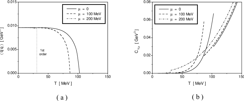
Figure 1: (a) Chiral condensate vs. temperature, and (b) specific heat $c_{{\mbox{\tiny\em V}},\mu}$ vs. temperature. Solid, dashed and dashed-dotted lines correspond to $\mu=0$, $\mu=100$ MeV and $\mu=200$ MeV respectively.

The result in Eq. (33) is useful to point out a generic feature of this type of models in the chiral limit. In fact, it is not difficult to show [13] that, in such limit, for zero $T$ and $\mu$ one obtains expressions for the pion decay constant $f_{\pi}^{(0)}$ and the chiral condensate $\langle\bar{q}q\rangle^{(0)}$ such that $f_{\pi}^{(0)}/\Lambda$ and $\langle\bar{q}q\rangle^{(0)}/\Lambda$ depend only on the combination $G\Lambda^{2}$. In order to get a ratio $f_{\pi}^{(0)}/\langle\bar{q}q\rangle^{(0)}\simeq 0.4$, as required by phenomenology, these expressions lead to $G\Lambda^{2}\simeq 16$. If this value is now replaced in Eq. (33) one gets $T_{c}(0)/\Lambda\simeq 0.12$, which is somewhat large, but still lies within the expected range of validity. However, if one imposes the critical temperature $T_{c}(0)$ to be approximately equal to 170 MeV, as suggested by lattice QCD calculations, one gets $\Lambda\simeq 1.4$ GeV, which, together with $G\Lambda^{2}\simeq 16$, enhances $f_{\pi}^{(0)}$ and $\langle\bar{q}q\rangle^{(0)}$ up to roughly 40% above the corresponding phenomenological values. Thus, it can be generically said that, if in the chiral limit —and within the mean field approximation— one wants to satisfy the phenomenological constraints on the values of $f_{\pi}$ and $\langle\bar{q}q\rangle$, the nonlocal models under consideration lead to a relatively low critical temperature $T_{c}(0)$. Of course, this might be modified by finite quark mass effects and/or beyond MFA corrections.

IV Phase transition and response functions for finite quark mass

In this Section we concentrate in the analysis of the phase transition for finite current quark masses in the isospin limit. For this purpose we will consider different thermodynamical response functions. In particular, it will be seen that, for reasonable values of the current quark mass $m_{c}$, the chiral susceptibilities show clear peaks that can be used to define the transition curves in the crossover region.

The response functions are basically given by the second derivatives of the Helmholtz free energy $F(T,V,\bar{N})$. The latter is related with the thermodynamical potential by

$$F(V,T,\bar{N})=\left[\Omega(V,T,\mu)+2\,\bar{N}\;\mu\right]_{\mu=\mu(V,T,\bar{N})}\ ,$$ (34)

where $\bar{N}=-\frac{1}{2}\;(\partial\Omega/\partial\mu)_{V,T}$ (as in the case of the quark condensate, the $\frac{1}{2}$ factor comes from defining $\bar{N}=\bar{N}_{u}=\bar{N}_{d}$). We will consider as before the limit of a large system in which $\Omega(V,T,\mu)=V\,\omega(T,\mu)$, $F(V,T,\bar{N})=V\,f(T,\bar{N}/V)$, thus instead of average particle number $\bar{N}$ our quantities will be given in terms of the average particle density $\rho=\bar{N}/V$. One can define three independent thermodynamical response functions, namely the specific heat at fixed volume and particle number $c_{{\mbox{\tiny\em V}},\rho,m}$, the isothermal compressibility $\kappa_{T,\rho,m_{c}}$ and the coefficient of thermal expansion $\alpha_{p,\rho,m_{c}}$. These are given by

$$c_{{\mbox{\tiny\em V}},\rho,m_{c}} = -\;\frac{T}{V}\left(\frac{\partial^{2}F(T,V,\bar{N},m_{c})}{\partial T^{2}}\right)_{V,\bar{N},m_{c}}=T\left(\frac{\partial s(T,\rho,m_{c})}{\partial T}\right)_{\rho,m_{c}}$$ (35)

$$\frac{1}{\kappa_{T,\rho,m_{c}}} = V\left(\frac{\partial^{2}F(T,V,\bar{N},m_{c})}{\partial V^{2}}\right)_{T,\bar{N},m_{c}}=\rho\left(\frac{\partial p(T,\rho,m_{c})}{\partial\rho}\right)_{T,m_{c}}$$ (36)

$$\alpha_{p,\rho,m_{c}} = \frac{1}{V}\left(\frac{\partial V}{\partial T}\right)_{p,\bar{N},m_{c}}=-\;\kappa_{T,\rho,m_{c}}\left(\frac{\partial^{2}F(T,V,\bar{N},m_{c})}{\partial V\;\partial T}\right)_{\bar{N},m_{c}}$$ (37)

$$= \kappa_{T,\rho,m_{c}}\left(\frac{\partial p(T,\rho,m_{c})}{\partial T}\right)_{\rho,m_{c}}$$

There are also other thermodynamical response functions that can be defined, such as the specific heat at constant pressure $c_{p,\rho,m_{c}}$ and the adiabatic compressibility $\kappa_{s,\rho,m_{c}}$. However, these can be written in terms of the three quantities in Eqs. (35-37).

Notice that we have explicitly included the dependence of the free energy on the current quark mass $m_{c}$. In fact, one can still define some extra response functions associated with the chiral transition by differentiating the free energy with respect to $m_{c}$. In the analogy with magnetic systems, these would be the specific heats at constant magnetization and constant applied magnetic field, $C_{M}$, $C_{H}$, the isothermal and adiabatic susceptibilities $\chi_{T}$, $\chi_{S}$, and the coefficient of thermal magnetization, $\alpha_{H}$. As before, these quantities are related to each other, leaving only two new independent response functions. Here we choose to consider those analogous to the isothermal susceptibility and the coefficient of thermal magnetization, thus we define

$$\chi_{{\mbox{\tiny\em V}},T,\rho} = -\;\frac{1}{2\,V}\;\left(\frac{\partial^{2}F(T,V,\bar{N},m_{c})}{\partial m_{c}^{2}}\right)_{T,V,\bar{N}}=-\;\left(\frac{\partial\langle\bar{q}q\rangle(T,\rho,m_{c})}{\partial m_{c}}\right)_{T,\rho}$$ (38)

$$\alpha_{{\mbox{\tiny\em V}},\rho,m_{c}} = -\;\frac{1}{2\,V}\;\left(\frac{\partial^{2}F(T,V,\bar{N},m_{c})}{\partial m_{c}\;\partial T}\right)_{V,\bar{N}}=-\;\left(\frac{\partial\langle\bar{q}q\rangle(T,\rho,m_{c})}{\partial T}\right)_{\rho,m_{c}}\ .$$ (39)

Let us show the numerical results for these quantities for the case of a nonlocal Gaussian regulator. We have chosen the parameter set $\Lambda=760$ MeV, $G=30$ GeV^-2 and $m_{c}=7.7$ MeV, which corresponds to Set II in the notation of Ref. [5]. It can be seen that these parameters lead to the empirical values of the pion mass and decay constant, and provide reasonable results for the chiral quark condensate and the quark selfenergy $\Sigma(0)$ at zero $T$ and $\mu$. In Fig. 2 we show the curves corresponding to the specific heat $c_{{\mbox{\tiny\em V}},\rho,m_{c}}$ and the chiral response functions $\chi_{{\mbox{\tiny\em V}},T,\rho}$ and $\alpha_{{\mbox{\tiny\em V}},\rho,m_{c}}$. In the left panels, these functions are plotted versus the temperature for three representative values of the density (the quoted values are referred to nuclear matter density, $\rho_{0}\simeq 1.3\times 10^{6}$ MeV³). Notice that for low nonzero densities the system is homogeneous only for temperatures which exceed a critical value. Below this limit, as we will see, there is a region where phases with broken and restored chiral symmetry coexist. In the right panels, the same response functions are plotted as functions of the density, fixing the temperature at 50 MeV and 100 MeV. Once again, for low temperatures there is a mixed phase region, and as a consequence the functions are not well defined at intermediate densities. We have also analyzed the response functions corresponding to the parameter set given by $G=50$ GeV^-2, $m_{c}=10.5$ MeV and $\Lambda=627$ MeV, or Set I in the notation of Ref. [5]. Set I and II might be interpreted as confining and nonconfining respectively, where confinement is understood in the sense that the pole structure of the quark propagator does not allow quarks to materialize on-shell in Minkowski space [12, 13]. The curves in the case of Set I do not differ qualitatively from those shown in Fig. 2, therefore they have not been included here.

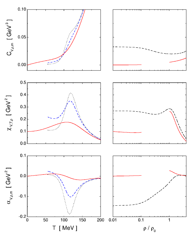
Figure 2: Some response functions for fixed $\rho$, corresponding to parameter Set II. In the left panels curves are given as functions of $T$, with $\rho/\rho_{0}$ fixed at three representative values, namely 0.25 (dotted), 0.75 (dashed) and 2.0 (solid). Right panels show the curves as functions of $\rho/\rho_{0}$ for $T$ fixed at 50 MeV (solid) and 100 MeV (dashed).

Now let us pay special attention to the responses of the chiral condensate (order parameter of the phase transition) at fixed temperature and chiral quark mass (or “magnetization”). These are given by Eqs. (38) and (39) and their behavior as functions of the temperature is shown in the second and third rows of Fig. 2 (left panels). As it is well known, susceptibilities are particularly useful to analyze the phase transition features. In the present model, as shown in previous works [4, 5], for low temperatures the system undergoes a first order chiral phase transition, which turns into a smooth crossover for temperatures exceeding a given “end point”. In this crossover region, the transition is characterized by the presence of respective peaks in the mentioned susceptibilities, the height and sharpness of these peaks giving a measure of the crossover steepness. The same can be observed if one looks at the chiral and thermal susceptibilities for fixed $\mu$, which are given by the second derivatives of the thermodynamical potential, and are in fact the natural quantities to deal with in the grand canonical ensemble. The definition of the chiral susceptibility $\chi_{{\mbox{\tiny\em V}},T,\mu}$ has been already given in Eq. (25), while the thermal susceptibility at constant $\mu$ is defined as

$$\alpha_{{\mbox{\tiny\em V}},\mu,m_{c}}\ =\ -\;\frac{1}{2}\;\left(\frac{\partial^{2}\omega(T,\mu,m_{c})}{\partial m_{c}\;\partial T}\right)_{\mu}=-\,\left(\frac{\partial\langle\bar{q}q\rangle(T,\mu,m_{c})}{\partial T}\right)_{\mu,m_{c}}\ .$$ (40)

The curves showing the behavior of the susceptibilities $\chi_{{\mbox{\tiny\em V}},T,\mu}$ and $\alpha_{{\mbox{\tiny\em V}},\mu,m}$ as functions of the temperature and the chemical potential are shown in Fig. 3 (the chosen parameter set is the same as in Fig. 2). For completeness we also include the curves for the specific heat at constant $\mu$, previously introduced in Sect. III (where the case of varying $m_{c}$ was discussed).

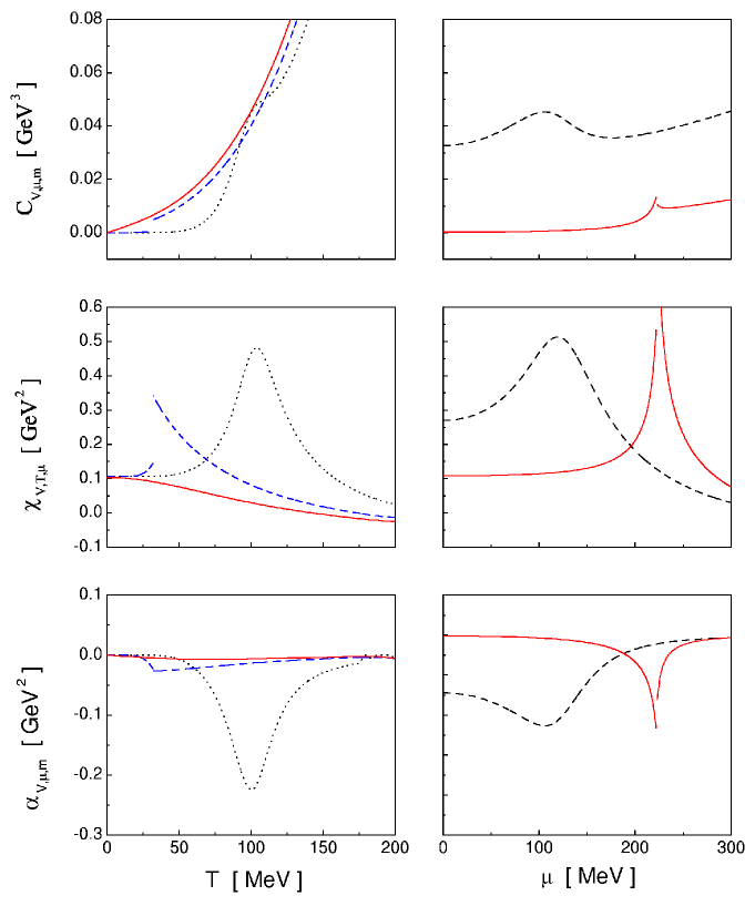
Figure 3: Some response functions for fixed $\mu$, corresponding to parameter Set II. In the left panels curves are given as functions of $T$, with $\mu$ fixed at three representative values, namely 100 MeV (dotted), 250 MeV (dashed) and 300 MeV (solid). Right panels show the curves as functions of $\mu$ for $T$ fixed at 50 MeV (solid) and 100 MeV (dashed).

In a natural way, the peaks in the curves for $\chi_{{\mbox{\tiny\em V}},T,\mu}$ and $\alpha_{{\mbox{\tiny\em V}},\mu,m_{c}}$ can be used to define the position at which the chiral transition occurs. Thus, one can extend the phase space diagram to include the crossover transition curves in addition to the first order ones. This is represented in Fig. 4, where crossover curves obtained from the peaks in $\chi_{{\mbox{\tiny\em V}},T,\mu}$ and $\alpha_{{\mbox{\tiny\em V}},\mu,m_{c}}$ have been represented by dashed and dotted lines respectively. Although chiral and thermal susceptibilities lead to slightly different points, it is seen that the transition region is well defined. Full lines correspond to the first order phase transition, while the fat dots indicate the end points. Left and right panels show the results for parameter Sets I and II respectively, while upper (lower) panels show the phase space transition curves in the $T-\mu$ ($T-\rho$) plane. Notice that in the $T-\rho$ phase diagrams there is a region below the first order transition lines where both phases are allowed. The latter can be interpreted [21] as a zone in which droplets containing light quarks of mass $m_{c}$ coexist with a gas of constituent, massive quarks. The dotted lines inside this zone are the spinodals, i.e. the boundaries of the region in which the energetically unfavored solutions can exist as metastable states.

Our results for the phase transition curves in the $T-\mu$ plane are qualitatively similar to those obtained from lattice QCD calculations [2, 3], although both the critical temperature at $\mu=0$ and the end point temperature turn out to be relatively low in our case (see discussion at the end of Sect. III). For the sake of comparison, it is also interesting to analyze the curvature of the phase boundary at $\mu=0$. This is an appropriate quantity to be studied in lattice QCD, where the main problem in the analysis of the $T-\mu$ phase diagram is the inclusion of a finite real chemical potential. Recent lattice calculations [1] yield $T_{c}(d^{2}T_{c}/d\mu^{2})|_{\mu=0}=-0.14\pm 0.06$, while the result obtained within the standard NJL model (up to some finite current quark mass corrections) gives a value of about $-0.40$  [22]. In our model, the curvature can be calculated numerically from the results plotted in Fig. 4, leading to values of about $-0.26$ and $-0.30$ for Sets I and II, respectively. In the chiral limit the corresponding calculation can be carried out from the analytical expression in Eq. (20), leading to $T_{c}(d^{2}T_{c}/d\mu^{2})|_{\mu=0}=-3/\pi^{2}\simeq-0.304$.

Figure 4: Phase diagram showing the chiral transition curves in the $T-\mu$ plane (upper panels) and the $T-\rho$ plane (lower panels), for parameter Sets I (left) and II (right). Solid lines correspond to first order phase transition curves, while dashed (dashed-dotted) lines show the crossover curves obtained from the peaks in the chiral (thermal) susceptibilities. The dotted lines in the lower panels represent the spinodals, and the fat dots indicate in each case the position of the end point.

Finally, let us quote the numerical results for the behavior of the energy density, the entropy density and the pressure as functions of the temperature. The corresponding curves are shown in Fig. 5, where we plot the scaled quantities $\varepsilon/T^{4}$, $\frac{3}{4}\,s/T^{3}$ and $3p/T^{4}$ versus the relative temperature $T/T_{c}$, for Sets I and II and different values of the chemical potential. The arrows indicate the value corresponding to a free fermion system in the large $T$ limit, given by $7\pi^{2}/10$ —see Eq. (18). Notice that for Set I there is a range of temperatures below $T_{c}$ for which all three quantities are negative. This might be taken as a further indication that for this parameter set there is a sort of “confinement”: somewhat below $T_{c}$ hadronic degrees of freedom ought to be included, and the system cannot be simply treated as a quark gas. This represents a qualitative difference between Sets I and II. It is interesting to see that, in spite of this fact, the behavior at the transition region is relatively similar in both cases.

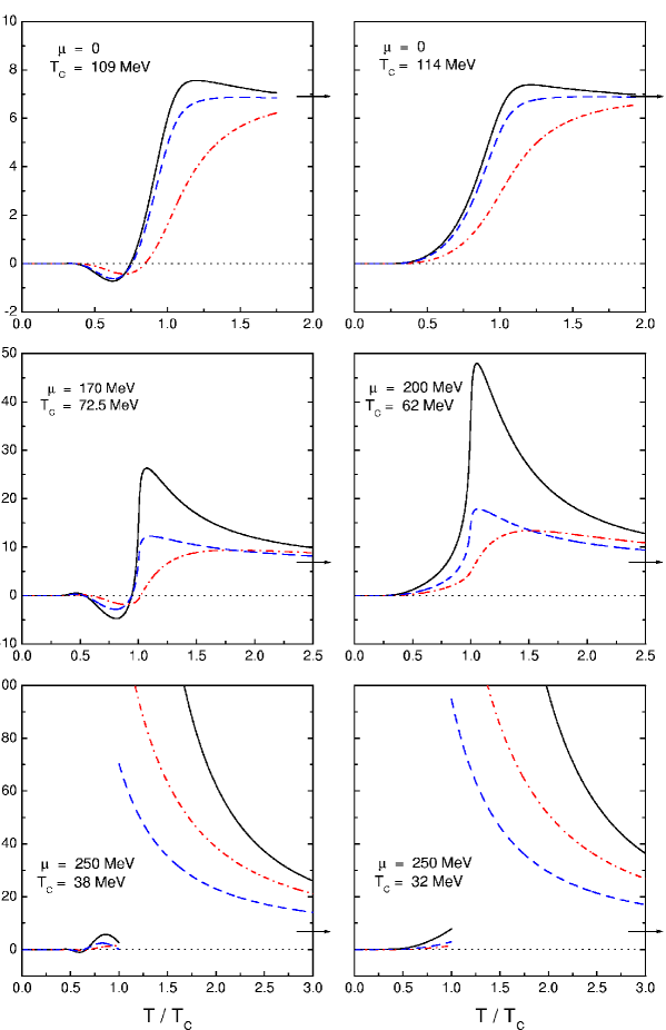
Figure 5: Numerical results for the scaled quantities $\varepsilon/T^{4}$ (solid), $\frac{3}{4}s/T^{3}$ (dashed) and $3p/T^{4}$ (dashed-dotted). Curves are given as functions of $T/T_{c}$, for fixed values of $\mu$ that are indicated in each case together with the respective critical temperatures. The arrows show the asymptotic values, which correspond to a free fermion system. Left and right panels show the results obtained for Sets I and II, respectively.

V Summary and outlook

In this work we have presented further details of the chiral phase transition within chiral quark models including nonlocal interactions in the mean field approximation. In the chiral limit, our analysis allows to obtain semi-analytical expressions for the transition curve and the location of the critical points. For the case of finite current quark masses, we have studied the behavior of various thermodynamical and chiral response functions across the phase transition. In the crossover region the thermal and chiral susceptibilities display clear peaks which allow to define a transition temperature, in the same way as it is usually done in lattice calculations.

The resulting phase diagrams are qualitatively similar to those obtained within other frameworks, as e.g. the standard NJL model, the Bag model, and lattice QCD. In the nonlocal schemes studied here, however, the transition temperature at $\mu=0$ is found to be somewhat lower than the expected value $T_{c}(0)\simeq 170$ MeV once the model parameters are fitted so as to reproduce both the empirical values of $m_{\pi}$ and $f_{\pi}$ and the phenomenological value of the light quark condensates at zero temperature and density. In fact, this result may be improved by considering alternative ways of including nonlocality, as e.g. regulator schemes inspired in one-gluon exchange processes [23], or through the inclusion of beyond MFA contributions. Work in this direction is currently in progress.

Appendix A: Expansion of the thermodynamical potential in powers of $\langle\bar{q}q\rangle$

The grand canonical thermodynamical potential defined by Eq. (11) turns out to be divergent. Here it has been regularized by subtracting the expression corresponding to a system of free fermions of mass $m_{c}$, and adding it in a regularized form. We have thus

$$\omega_{\mbox{\tiny\em MF}}^{(reg)}(T,\mu,m_{c})=\frac{\bar{\sigma}^{2}}{2G}\;-\ 4N_{c}\int\!\!\!\!\!\!\!\!\sum_{p}\ \log\left[\frac{p^{2}+\Sigma^{2}(p^{2})}{p^{2}+m_{c}^{2}}\right]+\omega_{free}^{(reg)}(T,\mu,m_{c})+\omega_{0}\ ,$$ (A.1)

where

$$\omega_{free}^{(reg)}(T,\mu,m_{c})=-\,4\,N_{c}\,T\int\frac{d^{3}p}{(2\pi)^{3}}\;\left[\,\log\left(1+e^{-(E-\mu)/T}\right)+\;\log\left(1+e^{-(E+\mu)/T}\right)\right]\;,$$ (A.2)

with $E=\sqrt{p^{2}+m_{c}^{2}}\,$, while $\omega_{0}$ is a constant fixed by imposing that the thermodynamical potential vanishes at zero $T$ and $\mu$. We point out that this regularization prescription relies on the well-behaved shape of the regulator in $\Sigma(p^{2})$. Alternative schemes can be applied in other cases, see e.g. [24].

Let us assume that in the chiral limit, $m_{c}=0$, the order parameter $\langle\bar{q}q\rangle$ vanishes at a given temperature $T=T_{c}$. We are interested in the description of the situation in the vicinity of this temperature, hence it is useful to carry out a double expansion of $\omega_{\mbox{\tiny\em MF}}^{(reg)}$ in powers of $\langle\bar{q}q\rangle$ and $m_{c}$. For $m_{c}=0$, the expansion of $\omega_{\mbox{\tiny\em MF}}^{(reg)}$ in powers of $\langle\bar{q}q\rangle$ can be performed by taking into account the derivatives

$$\left.\frac{\partial^{2}\omega_{\mbox{\tiny\em MF}}}{\partial\langle\bar{q}q\rangle^{2}}\;\right|_{\langle\bar{q}q\rangle=0} = \left.\frac{\partial^{2}\omega_{\mbox{\tiny\em MF}}}{\partial\sigma^{2}}\left(\frac{\partial\langle\bar{q}q\rangle}{\partial\sigma}\right)^{-2}\,\right|_{\langle\bar{q}q\rangle=0}$$

$$\left.\frac{\partial^{4}\omega_{\mbox{\tiny\em MF}}}{\partial\langle\bar{q}q\rangle^{4}}\;\right|_{\langle\bar{q}q\rangle=0} = \left.\frac{\partial^{4}\omega_{\mbox{\tiny\em MF}}}{\partial\sigma^{4}}\left(\frac{\partial\langle\bar{q}q\rangle}{\partial\sigma}\right)^{-4}-\ 4\ \frac{\partial^{2}\omega_{\mbox{\tiny\em MF}}}{\partial\sigma^{2}}\left(\frac{\partial\langle\bar{q}q\rangle}{\partial\sigma}\right)^{-5}\frac{\partial^{3}\langle\bar{q}q\rangle}{\partial\sigma^{3}}\;\right|_{\langle\bar{q}q\rangle=0}$$

$$\left.\frac{\partial\omega_{\mbox{\tiny\em MF}}}{\partial\langle\bar{q}q\rangle}\;\right|_{\langle\bar{q}q\rangle=0} = \left.\frac{\partial^{3}\omega_{\mbox{\tiny\em MF}}}{\partial\langle\bar{q}q\rangle^{3}}\;\right|_{\langle\bar{q}q\rangle=0}\ =\ \left.\frac{\partial^{5}\omega_{\mbox{\tiny\em MF}}}{\partial\langle\bar{q}q\rangle^{5}}\;\right|_{\langle\bar{q}q\rangle=0}\ =\ 0\ \ .$$ (A.3)

Since $\langle\bar{q}q\rangle=0$ implies $\sigma=0$, it is easy to see that the above partial derivatives are given by

$$\left.\frac{\partial\langle\bar{q}q\rangle}{\partial\sigma}\;\right|_{\sigma=0}=-\,4\,N_{c}\ S_{11}(T,\mu)\qquad \qquad\left.\frac{\partial^{3}\langle\bar{q}q\rangle}{\partial\sigma^{3}}\;\right|_{\sigma=0}=24\,N_{c}\ S_{32}(T,\mu)\ \ \ ;$$ ;

$$\left.\frac{\partial^{2}\omega_{\mbox{\tiny\em MF}}}{\partial\sigma^{2}}\;\right|_{\sigma=0}=\frac{1}{G}\,-\,8\,N_{c}\ S_{21}(T,\mu) \qquad\left.\frac{\partial^{4}\omega_{\mbox{\tiny\em MF}}}{\partial\sigma^{4}}\;\right|_{\sigma=0}=48\,N_{c}\ S_{42}(T,\mu)\ \ \ ,$$ ; (A.4)

where the functions $S_{mn}(T,\mu)$ are defined by

$$S_{mn}(T,\mu)\ =\ \int\!\!\!\!\!\!\!\!\sum_{p}\frac{r^{2m}(p^{2})}{p^{2n}}\ \ .$$ (A.5)

On the other hand, for $m_{c}\neq 0$ one has

$$\left.\frac{\partial\omega_{\mbox{\tiny\em MF}}}{\partial m_{c}}\;\right|_{m_{c}=0}=2\;\langle\bar{q}q\rangle\ .$$ (A.6)

Taking into account this relation, together with Eqs. (A.4) and (A.3), one easily arrives at the result shown in Eq. (15).

Appendix B: Evaluation of Matsubara sums

In this Appendix we will show how to work out the Matsubara sums $S_{m1}$ and $S_{m2}$, which are defined by Eq. (A.5). These sums appear in the Landau expansion of the thermodynamical potential near the critical temperature, see Eq. (15).

In order to carry out the calculations, we take into account the analysis in Ref. [5], where Cauchy’s theorem was used to convert the Matsubara sums into an integral plus a sum over pole residues. In the case of a function $F(p^{2})$ having only simple poles and no cuts in the complex plane one obtains [5]

$$\int\!\!\!\!\!\!\!\!\sum_{p}\ F(p^{2}) = \int\frac{d^{4}p}{(2\pi)^{4}}\ F(p^{2})\$$ (B.3)

$$+\ \ 2\int\frac{d^{3}p}{(2\pi)^{3}}\ \mbox{Re}\!\!\!\!\sum_{\scriptsize\begin{array}[]{cc}R_{k}>-\mu\\ I_{k}\geq 0\end{array}}\!\!\gamma_{k}\ \mbox{Res}\,[{\cal F}(z);z_{k}]\,\left[\,n_{+}(z_{k}+\mu)+n_{-}(z_{k}+\mu)\,\right]\,,$$

where the function ${\cal F}$ is defined as ${\cal F}(z)\equiv F[(-iz-i\mu)^{2}+|\vec{p}|^{2}]$, $z_{k}=R_{k}+iI_{k}$ are the residues of this function in the complex plane $z$, and the coefficient $\gamma_{k}$ is defined as $\gamma_{k}=1/2$ for $I_{k}=0$ and $\gamma_{k}=1$ otherwise. We have also introduced here (complex) occupation number functions $n_{\pm}(z)$, defined by

$$n_{\pm}(z)=\frac{1}{1+\exp\left[(z\mp\mu)/T\right]}\ \ .$$ (B.4)

In the case of the sum $S_{21}(T,\mu)$, the corresponding function ${\cal F}_{21}(z)$ is given by

$${\cal F}_{21}(z)\ =\ \frac{r_{\Lambda}^{4}[-(z+\mu)^{2}+|\vec{p}|^{2}]}{-(z+\mu)^{2}+|\vec{p}|^{2}}\ \ ,$$ (B.5)

which has only two simple poles located at $z^{\pm}=-\mu\pm|\vec{p}|$, with residues $\mp(2|\vec{p}|)^{-1}$. Therefore, Eq. (B.3) can in principle be applied. There is, however, an subtle point to be taken into account. The derivation of Eq. (B.3) assumes that $|{\cal F}(z)|\to 0$ when ${\rm Re\ }z\to\infty$, which is in fact true for all the situations considered in Ref. [5]. However, depending on the specific form of the regulator, this condition might be not satisfied by the function ${\cal F}_{21}(z)$. If this is the case, Eq. (B.3) can still be applied provided that $T,\mu\ll\Lambda$ (see below).

Assuming that Eq. (B.3) holds, one gets

$$S_{21}(T,\mu)\ =\ \int\!\!\!\!\!\!\!\!\sum_{p}\frac{r_{\Lambda}^{4}(p^{2})}{p^{2}}\ =\ \frac{1}{8\pi^{2}}\int_{0}^{\infty}\ dp\ p\ r_{\Lambda}^{4}(p^{2})-\ \frac{1}{4\pi^{2}}\int_{0}^{\infty}\ dp\ p\ [\,n_{+}(p)+n_{-}(p)\,]\ .$$ (B.6)

The last integral in this expression can be worked out analytically. One has

$$\int_{0}^{\infty}\ dp\ p\ [\,n_{+}(p)+n_{-}(p)\,]\ =\ -\;T^{2}\left[{\rm Li}_{2}(-e^{\mu/T})\;+\;{\rm Li}_{2}(-e^{-\mu/T})\right]\ =\ \frac{\pi^{2}\;T^{2}}{6}\ +\frac{\mu^{2}}{2}\ \ ,$$ (B.7)

which together with Eq. (B.6) leads to the result quoted in Eq. (20). As we have mentioned, this relations are only valid for sufficiently low values of $T,\mu$ compared with the cutoff scale $\Lambda$. In the case of the Gaussian regulator we have checked that for $T\leq\Lambda/6$ and $\mu\leq\Lambda/4$ Eq. (20) is verified with an accuracy of less that 1%. In the case of the Lorentzian regulator the region of validity is somewhat smaller, but at the same time the relevant cutoff parameter is larger than in the Gaussian case [5]. As a conclusion, we find that in all cases considered here Eq. (20) can be taken to be valid with very good approximation for the values of $T$ and $\mu$ of physical interest.

A similar analysis can be carried out for the sum $S_{42}(T,\mu)$. Here the situation is somewhat more complicated, since one has to deal with double poles and Eq. (B.3) is no longer valid. One has instead

$$S_{42}(T,\mu) = \int\!\!\!\!\!\!\!\!\sum_{p}\frac{r^{8}(p^{2})}{p^{4}}$$ (B.8)

$$= \int\frac{d^{4}p}{(2\pi)^{4}}\ F(p^{2})\ +\int\frac{d^{3}p}{(2\pi)^{3}}\ \left[\mbox{Res}\,\left(\frac{{\cal F}(z)}{1+e^{z/T}}\right)_{z^{+}}\!\!-\mbox{Res}\,\left(\frac{{\cal F}(z)}{1+e^{-z/T}}\right)_{z^{-}}\right]\;,$$

where $F(p^{2})=r_{\Lambda}^{8}(p^{2})/p^{4}$, ${\cal F}(z)=F(-(z+\mu^{2})+|\vec{p}|^{2})$. Evaluating the residues, this leads to

$$S_{42}(T,\mu) = \frac{1}{8\pi^{2}}\int_{0}^{\infty}\ dp\ \bigg{\{}\frac{1}{2\pi}\left(\int_{-\infty}^{\infty}dq\ \frac{r_{\Lambda}^{8}(p^{2}+q^{2})}{(p^{2}+q^{2})^{2}}\right)-\frac{1}{p}\left[n_{+}(p)+n_{-}(p)\,\right]$$ (B.9)

$$-\ 4\,m\ r_{\Lambda}^{\prime}(0)\ p\,[\,n_{+}(p)+n_{-}(p)\,]\ -\ \frac{1}{T}\,[\,n_{+}(p)+n_{-}(p)-n_{+}^{2}(p)-n_{-}^{2}(p)\,]\bigg{\}}\;,$$

where $r_{\Lambda}^{\prime}(0)=dr_{\Lambda}(p^{2})/dp^{2}|_{p^{2}=0}\;$. The first two terms lead to divergent integrals that can be worked out with the help of a definite regulator, e.g. the Gaussian one, writing

$$r_{\Lambda}^{8}(x^{2})=r_{\Lambda}^{8}(x^{2})-e^{-4x^{2}/\Lambda^{2}}+e^{-4x^{2}/\Lambda^{2}}\;.$$ (B.10)

For the Gaussian regulator, the sum of the divergent integrals in (B.9), properly regularized, is given by

$$\int_{0}^{\infty}\ dp\ \left\{\frac{1}{2\pi}\left(\int_{-\infty}^{\infty}dq\ \frac{e^{-4(p^{2}+q^{2})/\Lambda^{2}}}{(p^{2}+q^{2})^{2}}\right)-\frac{1}{p}\left[n_{+}(p)+n_{-}(p)\,\right]\right\} =$$ (B.11)

$$=\ \ \frac{1}{2}+\frac{\gamma}{2}-\log(\pi\sqrt{m})-\log\left(T/\Lambda\right)-f(\mu/T)\;,$$

where

$$f(x)\ =\ 2\;\sinh^{2}(x/2)\int_{0}^{\infty}\frac{dy}{y}\ \frac{\tanh(y/2)}{\cosh x+\cosh y}\ \ .$$ (B.12)

Finally, the integral of the last term in Eq. (B.9) can be explicitly performed, giving simply

$$\int_{0}^{\infty}\ dp\ [\;n_{+}(p)+n_{-}(p)-n_{+}^{2}(p)-n_{-}^{2}(p)\;]\ =\ T\ .$$ (B.13)

The previous result in Eq. (B.7), together with Eqs. (B.9) to (B.13), lead to the expression quoted in Eq. (30). Again this relation is strictly valid for $T,\mu\ll\Lambda$. For the Gaussian regulator we have checked that it still holds up to 1% in the region $T\leq\Lambda/9$, $\mu\leq\Lambda/5$. As before, this is also the case for the Lorentzian regulator for the values of $T$ and $\mu$ relevant for our analysis.

It is interesting to point out the similarity between our equations determining the second order transition line and the tricritical point, and those obtained in Ref. [20]. In that article, the authors address the study of the $T-\mu$ phase diagram using a different approach, in which they propose a large flavor number expansion and a resummed renormalization scheme. It can be seen that the results in Ref. [20] —Eqs. (13) and (14)— have the same form as our expressions if one takes the limit $\lambda=0$, which in the context of Ref. [20] means to neglect the contributions from the meson sector (this should be analogous to the MFA considered here). Moreover, the validity of these results is also limited to relatively low values of $T$ and $\mu$ in view of the presence of a Landau pole arising from the renormalization procedure.

References

- [1] C.R. Allton et al., Phys. Rev. D 68, 014507 (2003).
- [2] Z. Fodor and S.D. Katz, JHEP 0203, 014 (2002); JHEP 0404, 050 (2004).
- [3] F. Karsch and E. Laermann, arXiv:hep-lat/0305025.
- [4] I. General, D. Gómez Dumm, N.N. Scoccola, Phys. Lett. B 506, 267 (2001).
- [5] D. Gómez Dumm, N.N. Scoccola, Phys. Rev. D 65, 074021 (2002).
- [6] G. Ripka, Quarks bound by chiral fields (Oxford University Press, Oxford, 1997).
- [7] U. Vogl and W. Weise, Prog. Part. Nucl. Phys. 27, 195 (1991); S. Klevansky, Rev. Mod. Phys. 64, 649 (1992); T. Hatsuda and T. Kunihiro, Phys. Rep. 247, 221 (1994).
- [8] T. Schafer and E.V. Schuryak, Rev. Mod. Phys. 70, 323 (1998).
- [9] C.D. Roberts and A.G. Williams, Prog. Part. Nucl. Phys. 33, 477 (1994); C.D. Roberts and S.M. Schmidt, Prog. Part. Nucl. Phys. 45, S1 (2000).
- [10] E. Ruiz Arriola and L.L. Salcedo, Phys. Lett. B 450, 225 (1999).
- [11] G. Ripka, Nucl. Phys. A 683, 463 (2001); R.S. Plant and M.C. Birse, Nucl. Phys. A 703, 717 (2002).
- [12] M. Stingl, Phys. Rev. D 34, 3863 (1986) [Erratum-ibid. D 36, 651 (1987)]; H.J. Munczek, Phys. Lett. B 175, 215 (1986); C.J. Burden, C.D. Roberts and A.G. Williams, Phys. Lett. B 285, 347 (1992); G. Krein, C.D. Roberts and A.G. Williams, Int. J. Mod. Phys. A 7, 5607 (1992); D. Blaschke, G. Burau, Y.L. Kalinovsky, P. Maris and P.C. Tandy, Int. J. Mod. Phys. A 16, 2267 (2001).
- [13] R.D. Bowler and M.C. Birse, Nucl. Phys. A 582, 655 (1995); R.S.Plant and M.C. Birse, Nucl. Phys. A 628, 607 (1998).
- [14] A. Scarpettini, D. Gómez Dumm and N.N. Scoccola, Phys. Rev. D69, 114018 (2004).
- [15] W. Broniowski, B. Golli and G. Ripka, Nucl. Phys. A703, 667 (2002); A.H. Rezaeian, N.R. Walet and M.C. Birse, Phys. Rev. C 70, 065203 (2004).
- [16] R.S. Duhau, A.G. Grunfeld and N.N. Scoccola, Phys. Rev. D 70, 074026 (2004).
- [17] T.M. Schwarz, S.P. Klevansky and G. Papp, Phys. Rev. C 60, 055205 (1999).
- [18] See e.g. K. Huang, Statistical Mechanics, (J. Wiley & Sons, New York, 1987), Sec. 17.4.
- [19] D. Blaschke, A. Holl, C.D. Roberts and S.M. Schmidt, Phys. Rev. C 58, 1758 (1998); A. Holl, P. Maris and C.D. Roberts, Phys. Rev. C 59 1751 (1999).
- [20] A. Jakovác, A. Patkós, Zs. Szép and P. Szépfalusy, Phys. Lett. B 582, 179 (2004).
- [21] J. Berges and K. Rajagopal, Nucl. Phys. B 538, 215 (1999).
- [22] M. Buballa, Phys. Rept. 407, 205 (2005).
- [23] S.M. Schmidt, D. Blaschke and Y.L. Kalinovsky, Phys. Rev. C 50, 435 (1994).
- [24] D. Blaschke, C.D. Roberts and S.M. Schmidt, Phys. Lett. B 425, 232 (1998).