Axion Models with High-Scale Supersymmetry Breaking

Abstract

Inspired by the possibility of high-scale supersymmetry breaking in the string landscape where the cosmological constant problem and the gauge hierarchy problem can be solved while the strong CP problem is still a challenge for naturalness, we propose a supersymmetric KSVZ axion model with an approximate universal intermediate-scale ($\sim 10^{11}$ GeV) supersymmetry breaking. To protect the global Peccei–Quinn (PQ) symmetry against quantum gravitational violation, we consider the gauged discrete $Z_{N}$ PQ symmetry. In our model the axion can be a cold dark matter candidate, and the intermediate supersymmetry breaking scale is directly related to the PQ symmetry breaking scale. Gauge coupling unification can be achieved at about $2.7\times 10^{16}$ GeV. The Higgs mass range is 130 GeV to 160 GeV. We briefly discuss other axion models with high-scale supersymmetry breaking where the stabilization of the axion solution is similar.

I Introduction

There exists a great variety of structures for the superstring/M theory vacua, the ensemble of which is called the stringy “landscape” String . With the “weak anthropic principle” Weinberg , this proposal may not only give the first concrete explanation of the very tiny value of the cosmological constant which can only take discrete values, but also solve the gauge hierarchy problem. In particular, the supersymmetry breaking scale can be high if there exist many supersymmetry breaking parameters or many hidden sectors HSUSY ; NASD . Although there is no definite conclusion that the string landscape predicts high-scale or TeV-scale supersymmetry breaking HSUSY , it is interesting to study models with high-scale supersymmetry breaking NASD .

If supersymmetry is indeed broken at a high scale, the breaking scale can range from 1 TeV to the string scale. For simplicity, we consider three representative cases: (1) string-scale supersymmetry breaking, (2) intermediate-scale supersymmetry breaking, and (3) TeV-scale supersymmetry breaking. The TeV-scale supersymmetry has been studied extensively during the last two decades, so we do not discuss it here.

Although the original motivation for the New Minimal Standard Model (NMSM) Davoudiasl:2004be is different from the above string landscape argument, the NMSM provides a concrete model with string-scale supersymmetry breaking. With only six extra degrees of freedom beyond the minimal Standard Model (SM), the NMSM incorporates the new discoveries of physics beyond the minimal Standard Model: dark energy, non-baryonic dark matter, neutrino masses, as well as baryon asymmetry and cosmic inflation, by adopting the principle of minimal particle content and the most general renormalizable Lagrangian. The NMSM is free from excessive flavor-changing effects, CP violation, too-rapid proton decay, problems with electroweak precision data, and unwanted cosmological relics Davoudiasl:2004be . Moreover, gauge coupling unification can be achieved by considering threshold corrections Calmet:2004ck , or by introducing suitable additional particles, similar to the axion models with string-scale supersymmetry breaking that will be discussed in Section V. The unitarity constraints on couplings are weaker than the stability and triviality constraints Cynolter:2004cq .

For high-scale supersymmetry breaking, Arkani-Hamed and Dimopoulos proposed the split supersymmetry scenario where the scalars (squarks, sleptons and one combination of the scalar Higgs doublets) have masses at an intermediate scale, while the fermions (gauginos and Higgsinos) and the other combination of the scalar Higgs doublets are still at the TeV scale NASD . Gauge coupling unification is preserved and the lightest neutralino can still be a dark matter candidate. In addition, most of the problems with supersymmetric models, for example, flavor and CP violations, dimension-5 fast proton decay and the stringent constraints on the lightest Higgs mass, are solved. The consequences of split supersymmetry have been studied in Refs. GGAR ; SPLIT .

On the other hand, unlike the cosmological constant problem and the gauge hierarchy problem, the strong CP problem is still a concern in the string landscape Donoghue:2003vs . In the Standard Model, the $\overline{\theta}$ parameter is a dimensionless coupling constant which is infinitely renormalized by radiative corrections. There is no theoretical reason for $\overline{\theta}$ to be smaller than $10^{-9}$ as required by the experimental bound on the electric dipole moment of the neutron review ; pdg . There is also no known anthropic constraint on the value of $\overline{\theta}$, i.e., $\overline{\theta}$ may be a random variable with a roughly uniform distribution in the string landscape Donoghue:2003vs . An elegant and popular solution to the strong CP problem is provided by the Peccei–Quinn (PQ) mechanism PQ , in which a global axial symmetry $U(1)_{PQ}$ is introduced and broken spontaneously at some high energy scale. Then $\overline{\theta}$ is promoted to a dynamical field, $\overline{\theta}=a/f_{a}$, with an effective potential for this field induced by non-perturbative QCD effects. The axion $a$ is a pseudo-Goldstone boson from the spontaneous $U(1)_{PQ}$ symmetry breaking, with a decay constant $f_{a}$ (of similar scale as the $U(1)_{PQ}$ symmetry breaking scale). Minimization of the axion potential fixes the vacuum expectation value (VEV) of $a$, equivalently forces $\overline{\theta}$ to be zero, thus naturally solving the strong CP problem.

The original Weinberg–Wilczek axion WW is excluded by experiment, in particular by the non-observation of the rare decay $K\rightarrow\pi+a$ review . There are two viable “invisible” axion models in which the experimental bounds can be evaded: (1) the Kim–Shifman–Vainshtein–Zakharov (KSVZ) axion model, which introduces a SM singlet and a pair of extra vector-like quarks that carry $U(1)_{PQ}$ charges while the SM fermions and Higgs fields are neutral under $U(1)_{PQ}$ symmetry KSVZ ; (2) the Dine–Fischler–Srednicki–Zhitnitskii (DFSZ) axion model, in which a SM singlet and one pair of Higgs doublets are introduced, and the SM fermions and Higgs fields are charged under $U(1)_{PQ}$ symmetry DFSZ .

From laboratory, astrophysics, and cosmology constraints, the $U(1)_{PQ}$ symmetry breaking scale $f_{a}$ is limited to the range $10^{10}~{}{\rm GeV}\leq f_{a}\leq 10^{12}~{}{\rm GeV}$ review . Light axions can be produced in stars, and part of the star energy can be carried away by these axions. To avoid an unacceptable star energy loss, a lower bound is obtained on the axion decay constant, $f_{a}\geq 10^{10}$ GeV. During the course of cosmological evolution of the universe, the axions decouple early and begin to oscillate coherently. If $f_{a}$ is larger than about $10^{12}$ GeV, at some point in the evolution the energy density in the coherent axion oscillations could exceed the critical energy density and over-close the universe. The invisible axion can be a good cold dark matter candidate review .

In this paper we consider the axion models with high-scale supersymmetry breaking. Unlike split supersymmetry, we consider an approximately universal supersymmetry breaking, i.e., the mass differences among the squarks, sleptons, gauginos, Higgsinos and the $A$-terms are within one order of magnitude (within one-loop suppressions), which seems to be quite natural from flux-induced supersymmetry breaking Camara:2004jj .

We construct a supersymmetric KSVZ axion model where we introduce a SM singlet $S$ and two pairs of SM vector-like particles ($Q_{X}$, $\overline{Q}_{X}$) and ($D_{X}$, $\overline{D}_{X}$). The supersymmetry breaking scale and the Peccei–Quinn symmetry breaking scale are both around $10^{11}$ GeV, and the axion can be a cold dark matter candidate. We give the Higgs potential and the SM Yukawa couplings below the intermediate scale, the superpotential above the intermediate scale, and the matching conditions for the couplings. In addition, we consider the discrete $Z_{N}$ Peccei–Quinn symmetry, which can be embedded into an anomalous $U(1)_{A}$ gauge symmetry in string constructions where the anomalies can be cancelled by the Green–Schwarz mechanism MGJS . This $Z_{N}$ discrete symmetry cannot be violated by the quantum gravitational interaction. In order that the contributions to the $\overline{\theta}$ term from the non-renormalizable operators can be less than $10^{-9}$, we must require $N\geq~{}10$. We also show that a suitable quartic coupling for the singlet $S$ can be obtained at one-loop due to its large Yukawa couplings to the extra vector-like particles. Thus, the intermediate supersymmetry breaking scale is directly connected to the Peccei–Quinn symmetry breaking scale. Moreover, using two-loop renormalization group equation runnings for the gauge couplings and one-loop renormalization group equation runnings for the Yukawa couplings, we find that gauge coupling unification can be achieved at about $2.7\times 10^{16}$ GeV and the Higgs mass range is from 130 GeV to 160 GeV. Also, we calculate the Yukawa couplings for the third family of the SM fermions at the Grand Unified Theory (GUT) scale and comment on how to achieve Yukawa coupling unification. In our model, similar to the NMSM and split supersymmetry, most of the usual problems in the supersymmetric models are solved. If the $R$-parity is an exact symmetry, the lightest supersymmetric particle (LSP) neutralinos can be produced only non-thermally in a suitable amount, and their annihilations may have cosmological consequences. If $R$-parity is broken, the tiny masses and bilarge mixings for active neutrinos can be realized naturally at one-loop although we have to suppress the contributions to neutrino masses from the tree-level $\mu_{i}L_{i}H_{u}$ terms in the superpotential.

We also briefly discuss other axion models: the DFSZ axion model with intermediate-scale supersymmetry breaking where the stabilization of the axion solution and the Peccei–Quinn symmetry breaking are similar, the axion models with string-scale supersymmetry breaking, and the axion models with split supersymmetry.

II The KSVZ Axion Model with Intermediate-Scale
Supersymmetry Breaking

We first specify our conventions. We denote the left-handed quark doublets, the right-handed up-type quarks, the right-handed down-type quarks, the left-handed lepton doublets, the right-handed leptons, and the Higgs doublet in the Standard Model as $q_{i}$, $u_{i}$, $d_{i}$, $l_{i}$, $e_{i}$ and $H$, respectively, where $i$ is the family index. For the supersymmetric Standard Model, the SM fermions and Higgs fields are superfields belonging to chiral multiplets. We denote the left-handed quark doublets, the right-handed up-type quarks, the right-handed down-type quarks, the left-handed lepton doublets, the right-handed leptons, and one pair of Higgs doublets as $Q_{i}$, $U^{c}_{i}$, $D^{c}_{i}$, $L_{i}$, $E^{c}_{i}$, $H_{u}$ and $H_{d}$, respectively. The supersymmetry breaking scale is assumed to be at an intermediate scale in the range $10^{10}$ GeV to $10^{12}$ GeV. For simplicity, we assume that the gauginos, squarks, sleptons, Higgsinos, and one combination of the scalar Higgs doublets have a universal supersymmetry breaking soft mass ${\widetilde{M}}$.

We consider the KSVZ axion model KSVZ with a discrete Peccei–Quinn symmetry $Z_{N}$. This $Z_{N}$ symmetry can be realized after the anomalous $U(1)_{A}$ gauge symmetry is broken close to the string scale, where the $U(1)_{A}$ anomalies are cancelled by the Green–Schwarz mechanism MGJS , as will be discussed in the next Section. In the KSVZ axion model, the SM fermions and Higgs fields are assumed to be neutral under the $Z_{N}$ PQ symmetry. We introduce one SM singlet $S$ and two pairs of SM vector-like particles ($Q_{X}$, $\overline{Q}_{X}$) and ($D_{X}$, $\overline{D}_{X}$). Their quantum numbers under the SM $SU(3)_{C}\times SU(2)_{L}\times U(1)_{Y}$ gauge symmetry and the $Z_{N}$ symmetry are specified in Table 1. The axion potential from the QCD anomaly is generated when we couple the singlet $S$ to these extra vector-like particles. In addition, the charges of $Q_{X}$, $\overline{Q}_{X}$, $D_{X}$, $\overline{D}_{X}$, and $S$ under the $Z_{N}$ symmetry satisfy the relations

$$n_{Q_{X}}+n_{\overline{Q}_{X}}+n_{S} = 0~{}{\rm mod}~{}N~{},~{}\,$$ (1)

$$n_{D_{X}}+n_{\overline{D}_{X}}+n_{S} = 0~{}{\rm mod}~{}N~{}.~{}\,$$ (2)

Table 1: The quantum numbers for the superfields $Q_{X}$, $\overline{Q}_{X}$, $D_{X}$, $\overline{D}_{X}$, and $S$ under the $SU(3)_{C}\times SU(2)_{L}\times U(1)_{Y}\times Z_{N}$ symmetry.

Superfields	Quantum Numbers	Superfields	Quantum Numbers
$Q_{X}$	(3, 2, 1/6, ${\bf n_{Q_{X}}}$)	$\overline{Q}_{X}$	(${\bf\overline{3}}$, 2, $-$1/6, ${\bf n_{\overline{Q}_{X}}}$)
$D_{X}$	(3, 1, $-$1/3, ${\bf n_{D_{X}}}$)	$\overline{D}_{X}$	(${\bf\overline{3}}$, 1, 1/3, ${\bf n_{\overline{D}_{X}}}$)
$S$	(1, 1, 0, ${\bf n_{S}}$)

In our model the two pairs of the SM vector-like particles ($Q_{X}$, $\overline{Q}_{X}$) and ($D_{X}$, $\overline{D}_{X}$) have masses comparable to the universal supersymmetry breaking soft mass ${\widetilde{M}}$ after the supersymmetry and Peccei-Quinn symmetry breakings. Below the scale ${\widetilde{M}}$ we assume that only one scalar Higgs doublet $H$ is light as arranged by suitable fine-tuning. Thus, besides the gauge kinetic terms for all the fields, the most general renormalizable Lagrangian at tree-level is

$${\cal L} = m_{H}^{2}H^{\dagger}H-\frac{\lambda}{2!}\left(H^{\dagger}H\right)^{2}-\left[h^{u}_{ij}{\bar{q}}_{j}u_{i}\epsilon H^{*}+h^{d}_{ij}{\bar{q}}_{j}d_{i}H+h^{e}_{ij}{\bar{\ell}}_{j}e_{i}H+{\rm H.C.}\right]~{},~{}\,$$ (3)

where $m_{H}^{2}$ is the squared Higgs mass, $\lambda$ is the Higgs quartic coupling, $\epsilon\equiv i\sigma^{2}$ where $\sigma^{2}$ is the second Pauli matrix, and $h^{u}_{ij}$, $h^{d}_{ij}$, and $h^{e}_{ij}$ are the Yukawa couplings.

The Lagrangian in Eq. (3) is obtained after the gauginos, squarks, sleptons, Higgsinos, and one combination of the scalar Higgs doublets from $H_{u}$ and $H_{d}$ in the supersymmetric model are decoupled at the scale $\widetilde{M}$. Matching the Lagrangian in Eq. (3) with the supersymmetric interaction terms for the Higgs doublets $H_{u}$ and $H_{d}$, we obtain the relevant Lagrangian in terms of the coupling constants in the SM at the scale $\widetilde{M}$

$${\cal L}_{\rm SUSY} = -\frac{g_{2}^{2}}{8}\left(H_{u}^{\dagger}\sigma^{i}H_{u}+H_{d}^{\dagger}\sigma^{i}H_{d}\right)^{2}-\frac{g_{Y}^{2}}{8}\left(H_{u}^{\dagger}H_{u}-H_{d}^{\dagger}H_{d}\right)^{2}$$ (4)

$$+\left[y^{u}_{ij}H_{u}\epsilon{\bar{u}}_{i}q_{j}-y^{d}_{ij}H_{d}\epsilon{\bar{d}}_{i}q_{j}-y^{e}_{ij}H_{d}\epsilon{\bar{e}}_{i}\ell_{j}+{\rm H.C.}\right]~{},~{}\,$$

where $\sigma^{i}$ are the Pauli matrices, $g_{2}$ and $g_{Y}$ are respectively the gauge couplings for the $SU(2)_{L}$ and $U(1)_{Y}$ groups, and $y^{u}_{ij}$, $y^{d}_{ij}$, and $y^{e}_{ij}$ are the Yukawa couplings at and above scale $\widetilde{M}$. Here we neglect the Yukawa couplings for the extra vector-like particles that will be given later in Eq. (7).

From the scalar Higgs doublets in the chiral multiplets, $H_{u}$ and $H_{d}$, we define the SM Higgs doublet combination as $H\equiv-\cos\beta\epsilon H_{d}^{*}+\sin\beta H_{u}$ which is fine-tuned to have a small mass term, while the other combination ($\sin\beta\epsilon H_{d}^{*}+\cos\beta H_{u}$) has mass around ${\widetilde{M}}$ NASD . Therefore, we obtain the coupling constants in Eq. (3) at the scale $\widetilde{M}$ from those in Eq. (4) by the replacements $H_{u}\to\sin\beta H$ and $H_{d}\to\cos\beta\epsilon H^{*}$

$$\lambda(\widetilde{M}) = \frac{\left[g_{2}^{2}(\widetilde{M})+3g_{1}^{2}(\widetilde{M})/5\right]}{4}\cos^{2}2\beta~{},~{}\,$$ (5)

$$h^{u}_{ij}(\widetilde{M})=(y^{u}_{ij})^{*}(\widetilde{M})\sin\beta, h^{d,e}_{ij}(\widetilde{M})=(y^{d,e}_{ij})^{*}(\widetilde{M})\cos\beta~{},~{}\,$$ (6)

where we assume the $SU(5)$ normalization for the gauge coupling of $U(1)_{Y}$, i.e., $g_{1}^{2}\equiv(5/3)g_{Y}^{2}$.

Above the scale ${\widetilde{M}}$ the theory is supersymmetric. The superpotential in our model is

$$W = y^{u}_{ij}H_{u}\epsilon U^{c}_{i}Q_{j}-y^{d}_{ij}H_{d}\epsilon D^{c}_{i}Q_{j}-y^{e}_{ij}H_{d}\epsilon E^{c}_{i}L_{j}+y_{Q_{X}}SQ_{X}\overline{Q}_{X}$$ (7)

$$+y_{D_{X}}SD_{X}\overline{D}_{X}+y_{S}{{S^{N}}\over\displaystyle{M_{Pl}^{N-3}}}~{},~{}\,$$

where $y_{Q_{X}}$, $y_{D_{X}}$ and $y_{S}$ are the Yukawa couplings for the extra particles, and $M_{Pl}$ is the Planck scale. The last term, $y_{S}S^{N}/M_{Pl}^{N-3}$, is the lowest possible higher dimensional operator for the singlet $S$; this operator is related to the destabilization of the axion solution and suppressed by the Planck scale. Consequently, in the following discussions we do not consider the renormalization group evolution for the coupling $y_{S}$ and neglect it in our renormalization group equations.

III Stabilization of the Axion Solution and Peccei–Quinn
Symmetry Breaking

Quantum gravitational effects, associated with black holes, worm holes, etc., are believed to violate all the global symmetries, while they respect all the gauge symmetries Hawking . These effects may destabilize the axion solution to the strong CP problem due to the violation of the global Peccei–Quinn symmetry. However, after a gauge symmetry is spontaneously broken, there may exist a remnant discrete gauge symmetry which will not be violated by quantum gravity LKFW . Thus, a possible way to avoid the destabilization problem associated with quantum gravity is to identify the Peccei–Quinn symmetry as an approximate global symmetry arising from the broken gauge symmetry.

In weakly coupled heterotic string model building, there generically exists an anomalous $U(1)_{A}$ gauge symmetry with its anomalies cancelled by the Green–Schwarz mechanism MGJS . For Type II orientifold string model building, there may exist more than one anomalous $U(1)_{A}$ gauge symmetry whose anomalies can be cancelled by the generalized Green–Schwarz mechanism Aldazabal:2000dg . The anomalous $U(1)_{A}$ gauge symmetry is broken near the string scale when some scalar fields, which are charged under $U(1)_{A}$, obtain VEVs and cancel the Fayet–Iliopoulos term of $U(1)_{A}$. Then the D-flatness for $U(1)_{A}$ is preserved and the supersymmetry is unbroken DSW . Usually, there is an unbroken discrete $Z_{N}$ subgroup of the $U(1)_{A}$ gauge symmetry, which is protected against quantum gravitational violation. We shall consider this $Z_{N}$ discrete symmetry as an approximate global $U(1)_{PQ}$ symmetry Babu:2002ic .

For the gauge symmetry $\prod_{i}G_{i}\times U(1)_{A}$, the Green–Schwarz anomaly cancellation conditions from an effective theory point of view are TBMD ; Ibanez

$$\frac{A_{i}}{k_{i}}=\frac{A_{gravity}}{12}=\delta_{GS}~{},~{}\,$$ (8)

where the $A_{i}$ are anomaly coefficients associated with $G_{i}^{2}\times U(1)_{A}$, $k_{i}$ is the level of the corresponding Kac–Moody algebra, and $\delta_{GS}$ is a constant which is not specified by low-energy theory alone. For a non-Abelian group, $k_{i}$ is a positive integer, while for the $U(1)$ gauge symmetry, $k_{i}$ need not be an integer. All the other anomaly coefficients such as $G_{i}G_{j}G_{k}$ and $[U(1)_{A}]^{2}\times G_{i}$ should vanish.

In our model the gauge symmetry in which we are interested is $SU(3)_{C}\times SU(2)_{L}\times U(1)_{Y}\times U(1)_{A}$. Because the SM fermions and Higgs fields are not charged under $U(1)_{A}$, there are no anomalies from them. Thus, we only need to consider the anomalies from the two pairs of SM vector-like fields ($Q_{X}$, $\overline{Q}_{X}$) and ($D_{X}$, $\overline{D}_{X}$) that involve at least one $U(1)_{A}$.

For simplicity, we assume that $n_{Q_{X}}=n_{D_{X}}$ and $n_{\overline{Q}_{X}}=n_{\overline{D}_{X}}$. Using the Georgi–Glashow $SU(5)$ normalization Georgi:1974sy , we find that the $U(1)_{Y}[U(1)_{A}]^{2}$ anomaly vanishes and that the $[U(1)_{Y}]^{2}\times U(1)_{A}$, $[SU(2)_{L}]^{2}\times U(1)_{A}$ and $[SU(3)_{C}]^{2}\times U(1)_{A}$ anomaly coefficients $A_{1}$, $A_{2}$ and $A_{3}$ are

$$5A_{1}=A_{2}=A_{3}={3\over 2}\left(n_{Q_{X}}+n_{\overline{Q}_{X}}\right)~{}.$$ (9)

Thus, the anomalies can be cancelled by choosing the $k_{i}$ as follows

$$k_{1}={1\over 5}~{},~{}k_{2}=k_{3}=1~{}.~{}\,$$ (10)

Usually, one only considers non-Abelian anomaly cancellations because the associated Kac–Moody level for $U(1)$ is not an integer in general, hence this condition is not very useful from a low-energy effective theory point of view Babu:2002ic ; TBMD .

In addition, we can have models with $k_{1}=k_{2}=k_{3}=1$, although we have to introduce more particles. Let us give an explicit example. To ensure gauge coupling unification, we introduce two pairs of SM vector-like fields with quantum numbers ((${\bf 3},{\bf 2},{\bf 1/6}$), (${\bf\overline{3}}$, ${\bf 2}$, ${\bf-1/6}$)) and ((${\bf 3}$, ${\bf 1}$, ${\bf-1/3}$), (${\bf\overline{3}}$, ${\bf 1}$, ${\bf 1/3}$)). An alternative way to achieve gauge coupling unification is to introduce two chiral multiplets with quantum numbers (${\bf 8},{\bf 1},{\bf 0}$) and (${\bf 1},{\bf 3},{\bf 0}$), and one pair of SM vector-like particles with quantum numbers ((${\bf 1}$, ${\bf 2}$, ${\bf-1/2}$), (${\bf 1}$, ${\bf 2}$, ${\bf 1/2}$)). In these two cases, all the extra particles are neutral under $U(1)_{A}$ and have masses around $10^{11}$ GeV, and the gauge coupling unification scale is about $2\times 10^{16}$ GeV. To realize the KSVZ axion and preserve the gauge coupling unification, we introduce at least one pair of SM vector-like fields with $SU(5)$ quantum numbers, for instance, ($\bf 5$, $\bf\overline{5}$) or ($\bf 10$, $\bf\overline{10}$), that are charged under $U(1)_{A}$ and can couple to the singlet $S$ via superpotential $S{\bf 5}{\bf\overline{5}}$ or $S{\bf 10}{\bf\overline{10}}$ terms. Because these SM vector-like fields, which couple to $S$ and give the axion potential from QCD anomaly, form a complete $SU(5)$ representation, we have $k_{1}=k_{2}=k_{3}=1$. However, this model is not economical compared to above model because we need to add more particles.

To ensure that the contributions to the $\overline{\theta}$ term from the non-renormalizable operators are less than $10^{-9}$, we constrain the order $N$ of the $Z_{N}$ symmetry. The most dangerous term is the following hard supersymmetry breaking term in the potential:

$$V_{SB} = A_{y_{S}}y_{S}{{S^{N}}\over\displaystyle{M_{Pl}^{N-3}}}+{\rm H.C.}~{},~{}\,$$ (11)

where $A_{y_{S}}$ can be complex. This term would induce a non-zero contribution to $\overline{\theta}$ Barr of

$$\Delta\overline{\theta}~{}\simeq~{}A_{y_{S}}y_{S}\frac{f_{a}^{N}}{{M_{Pl}}^{N-3}\Lambda_{QCD}^{4}}~{}.$$ (12)

Here we assumed that CP violation is of order 1 so that there is no extra fine-tuning in our discussion.

For numerical calculations, we first evaluate $f_{a}$. Assuming that the ratio of the axion number density to the entropy density has been constant since the axion acquired mass and started to oscillate, we have Sikivie:1999sy

$$\Omega_{a}h^{2}\simeq\left({{f_{a}}\over\displaystyle{10^{12}~{}{\rm GeV}}}\right)^{7/6}\left({{200~{}{\rm MeV}}\over\displaystyle{\Lambda_{QCD}}}\right)^{3/4}~{}.~{}\,$$ (13)

Using the dark matter relic density of $\Omega_{a}h^{2}\simeq 0.1126$ from the WMAP analysis Spergel:2003cb and taking $\Lambda_{QCD}=200$ MeV, we obtain $f_{a}\simeq 1.54\times 10^{11}$ GeV.

Assuming that $y_{S}=1$ and requiring that $\Delta\overline{\theta}<10^{-9}$, we obtain

$$\left\{\begin{array}[]{ll}N\geq 11,&~{}~{}~{}~{}~{}~{}{\rm for}~{}~{}A_{y_{S}}\sim 10^{11}~{}{\rm GeV}\\ N\geq 10,&~{}~{}~{}~{}~{}~{}{\rm for}~{}~{}A_{y_{S}}\sim 10^{4}~{}{\rm GeV}\end{array}\right.\ ~{},~{}\,$$ (16)

where we take $M_{Pl}=2.4\times 10^{18}$ GeV. If the CP violation phase or the magnitude of $A_{y_{S}}$, or the coupling $y_{S}$ are very small, the values $N$ can be smaller than these lower bounds.

The above stabilization discussion is generic for supersymmetric axion models because the hard supersymmetry breaking terms can be induced from the non-renormalizable operators in the Kähler potential after supersymmetry breaking. For example, in our model we can have the following non-renormalizable operator in the Kähler potential

$$S = \int d^{4}xd^{4}\theta\left({{y_{ZS}Z^{\dagger}ZS^{N}}\over\displaystyle{M_{*}^{N}}}+{\rm H.C.}\right)~{},~{}\,$$ (17)

where $y_{ZS}$ is a coupling constant, and $Z$ is a spurion superfield which parametrizes the supersymmetry breaking via $\langle F_{Z}\rangle\not=0$. For simplicity, we assume that the mass scale $M_{*}$ is equal to the Planck scale $M_{Pl}$ and $\langle F_{Z}\rangle/M_{Pl}$ is about $10^{11}$ GeV. Therefore, we obtain

$$A_{y_{S}}={{y_{ZS}}\over{y_{S}}}{{|F_{Z}|^{2}}\over{M_{Pl}^{3}}}\sim{{y_{ZS}}\over{y_{S}}}\times 10^{4}~{}{\rm GeV}~{}.~{}\,$$ (18)

Using $y_{ZS}\sim 1$ and $y_{S}\sim 1$, we obtain $N\geq 10$.

In general, suppose we have several singlets $S_{i}$ that are charged under the $Z_{N}$ symmetry whose VEVs are comparable to that of $S$, and suppose that the lowest dimensional operator allowed by the gauge symmetry and $Z_{N}$ symmetry is $S^{n_{0}}\prod_{i}S_{i}^{n_{i}}$, where $n_{0}$ is a positive integer and $n_{i}$ are non-negative integers. To ensure that the contribution to the $\overline{\theta}$ term from this operator is naturally less than $10^{-9}$, we require

$$n_{0}+\sum_{i}n_{i}\geq 11~{}{\rm or}~{}10~{}.~{}\,$$ (19)

We next discuss Peccei–Quinn symmetry breaking. Because the soft mass and the VEV of the singlet $S$ are about $10^{11}$ GeV, we have to generate a suitable quartic coupling for $S$ at one-loop from the two pairs of SM vector-like fields. This can be realized as long as $y_{Q_{X}}$ and $y_{D_{X}}$ are of order 1. The one-loop effective potential for $S$ is

$$V_{eff} = -{\tilde{m}}^{2}_{S}|S|^{2}-{3\over{8\pi^{2}}}y_{Q_{X}}^{4}|S|^{4}\left({\rm log}{{y_{Q_{X}}^{2}|S|^{2}}\over{Q^{2}}}-{3\over 2}\right)-{3\over{16\pi^{2}}}y_{D_{X}}^{4}|S|^{4}\left({\rm log}{{y_{D_{X}}^{2}|S|^{2}}\over{Q^{2}}}-{3\over 2}\right)$$ (20)

$${}+{3\over{8\pi^{2}}}\left({\tilde{m}}_{Q_{X}}^{2}+y_{Q_{X}}^{2}|S|^{2}\right)^{2}\left({\rm log}{{{\tilde{m}}_{Q_{X}}^{2}+y_{Q_{X}}^{2}|S|^{2}}\over{Q^{2}}}-{3\over 2}\right)$$

$${}+{3\over{16\pi^{2}}}\left({\tilde{m}}_{D_{X}}^{2}+y_{D_{X}}^{2}|S|^{2}\right)^{2}\left({\rm log}{{{\tilde{m}}_{D_{X}}^{2}+y_{D_{X}}^{2}|S|^{2}}\over{Q^{2}}}-{3\over 2}\right)~{},~{}\,$$

where ${\tilde{m}}^{2}_{S}$ is the soft supersymmetry breaking mass for $S$, ${\tilde{m}}_{Q_{X}}^{2}$ is the soft mass for $Q_{X}$ and $\overline{Q}_{X}$, and ${\tilde{m}}_{D_{X}}^{2}$ is the soft mass for $D_{X}$ and $\overline{D}_{X}$; $Q$ is the renormalization scale, which is about $f_{a}$ here. Approximately, the quartic term for $S$ is

$$V_{eff}\supset{{\lambda_{S}}\over{2!}}(S^{\dagger}S)^{2}~{},~{}\,$$ (21)

where

$$\lambda_{S}={3\over{4\pi^{2}}}y_{Q_{X}}^{4}{\rm log}\left({{{\tilde{m}}_{Q_{X}}^{2}}\over{y_{Q_{X}}^{2}f_{a}^{2}}}+1\right)+{3\over{8\pi^{2}}}y_{D_{X}}^{4}{\rm log}\left({{{\tilde{m}}_{D_{X}}^{2}}\over{y_{D_{X}}^{2}f_{a}^{2}}}+1\right)~{}.~{}\,$$ (22)

For $y_{Q_{X}}=y_{D_{X}}=0.8$ and ${\tilde{m}}_{Q_{X}}={\tilde{m}}_{D_{X}}=5f_{a}$, we obtain $\lambda_{S}=0.17$.

We emphasize that for a supersymmetry breaking scale higher than $10^{12}$ GeV, the VEV of $S$ around $f_{a}\sim 1.54\times 10^{11}$ GeV may not be natural. For a supersymmetry breaking scale lower than $10^{10}$ GeV, one may not be able to generate the suitable quartic coupling for the singlet $S$ naturally. Therefore, the Peccei–Quinn symmetry can be broken naturally if and only if the supersymmetry breaking scale is intermediate, i.e., from $10^{10}$ GeV to $10^{12}$ GeV, and then the intermediate supersymmetry breaking scale is directly related to the Peccei–Quinn symmetry breaking scale.

IV Gauge Coupling Unification and Phenomenology

IV.1 Gauge Coupling Unification

We next consider gauge coupling unification. The two-loop renormalization group equations for the gauge couplings and the one-loop renormalization group equations for the Yukawa couplings are given in Appendix A. The renormalization group equation runnings are logarithmic and we shall neglect the uncertainties from threshold corrections. For simplicity, we consider the universal supersymmetry breaking mass ${\widetilde{M}}$ for the superpartners of the SM particles, and we assume that the masses for the two pairs of SM vector-like superfields ($Q_{X}$, $\overline{Q}_{X}$) and ($D_{X}$, $\overline{D}_{X}$) are the same and given by $m_{X}$.

In numerical calculations we use the following initial values at the $M_{Z}$ scale in Ref. Eidelman:2004wy :

$$\alpha^{-1}(M_{Z})=128.91\pm 0.02\,,$$

$$\sin^{2}\theta_{W}(M_{Z})=0.23120\pm 0.00015\,,$$

$$M_{Z}=91.1876\pm 0.0021\,{\rm GeV}\,,$$

$$v=174.10\,{\rm GeV}\,,$$ (23)

along with a top quark pole mass $m_{t}=178.\pm 4.3$ GeV Azzi:2004rc and $\alpha_{s}(M_{Z})=0.1182\pm 0.0027$ Bethke:2004uy . We choose $m_{X}=1.0\times 10^{11}$ GeV, and $y_{Q_{X}}=y_{D_{X}}=0.8$ at the $m_{X}$ scale. The supersymmetry breaking scale $\widetilde{M}$ and the GUT scale $M_{GUT}$ are determined by requiring the gauge couplings to unify at $M_{GUT}$. For the ${\overline{MS}}$ top quark Yukawa coupling, we use the one-loop corrected value Arason:1991ic , which is related to the top quark pole mass by

$$m_{t}=h_{t}v\left(1+\frac{16}{3}\frac{g_{3}^{2}}{16\pi^{2}}-2\frac{h_{t}^{2}}{16\pi^{2}}\right)\,.$$ (24)

The unifications of the gauge couplings for $\tan\beta=1.5$ and $\tan\beta=50$ are shown in Fig. 1, in which the supersymmetry breaking scale $\widetilde{M}$ is $1.4\times 10^{10}$ GeV. The GUT scale $M_{GUT}$ is about $2.6\times 10^{16}$ GeV and $2.7\times 10^{16}$ GeV for $\tan\beta=1.5$ and $\tan\beta=50$, respectively. The supersymmetry breaking scale, the GUT scale, and the unified gauge coupling are almost independent of $\tan\beta$.

Figure 1: Gauge coupling unifications for $\tan\beta=1.5$ (left) and $\tan\beta=50$ (right).

We point out that if the gauginos and Higgsinos have masses of about $\widetilde{M}$ while the squarks and sleptons are about one order of magnitude heavier, the gauge coupling unification scale is the same as above because the squarks and sleptons form complete $SU(5)$ representations.

IV.2 Higgs Mass

To calculate the Higgs mass, we first evaluate the Higgs quartic coupling $\lambda$ at the scale $\widetilde{M}$ and then evolve it down to the $M_{Z}$ scale. The effective potential, with the top quark radiative correction included, is

$$V_{eff}=m_{h}^{2}H^{\dagger}H-\frac{\lambda}{2!}(H^{\dagger}H)^{2}-\frac{3}{16\pi^{2}}h_{t}^{4}(H^{\dagger}H)^{2}\left[\log\frac{h_{t}^{2}(H^{\dagger}H)}{Q^{2}}-\frac{3}{2}\right]\,.$$ (25)

We derive the Higgs mass by minimizing the effective potential. The scale $Q$ is chosen to be at the Higgs mass. We show the predicted Higgs mass as a function of $\tan\beta$ in Fig. 2. The upper, center and lower groups of curves correspond to the top quark mass being $(178.0+4.3)$ GeV, $178.0$ GeV and $(178.0-4.3)$ GeV, respectively. Within each group, the upper and lower curves show the uncertainty due to the $1\sigma$ uncertainty of $\alpha_{s}$. The lower curve is generated with $\alpha_{s}=0.1182+0.0027$ and the upper with $\alpha_{s}=0.1182-0.0027$.

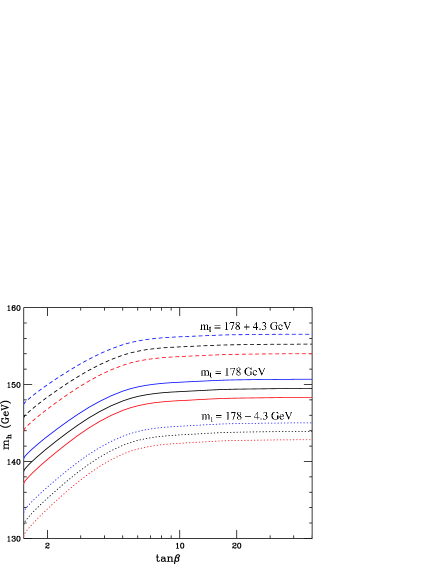
Figure 2: The Higgs mass versus $\tan\beta$. The group of solid curves are results for $m_{t}=178.0$ GeV, the dashed for $m_{t}=178.0+4.3$ GeV, and the dotted for $m_{t}=178.0-4.3$ GeV. Within each group, the center curve is generated with $\alpha_{s}=0.1182$, the lower curve with $\alpha_{s}=0.1182+0.0027$, and the upper with $\alpha_{s}=0.1182-0.0027$.

Below the scale $\widetilde{M}$, the Higgs boson is just as in the SM. A SM Higgs boson in the mass range 130–160 GeV can be identified at the $3\sigma$ level of significance with $30~{}{\rm fb}^{-1}$ integrated luminosity at the Tevatron Han:1998ma ; Carena:2000yx . At the LHC, the Higgs boson in this mass range can be discovered in the $\gamma\gamma$ and the $\tau^{+}\tau^{-}$ channels with $100~{}{\rm fb}^{-1}$ of data Higgs_LHC .

IV.3 Top, Bottom and Tau Yukawa Couplings at the GUT Scale

Besides gauge coupling unification, it is also interesting to study whether there exists Yukawa coupling unification for the top ($t$) quark, the bottom ($b$) quark and the $\tau$ lepton at the GUT scale. The ratios of the Yukawa couplings ($y_{t}/y_{\tau}$, $y_{t}/y_{b}$ and $y_{b}/y_{\tau}$) as a function of $\tan\beta$ are shown in Fig. 3.

Figure 3: The ratios of Yukawa couplings at the GUT scale versus $\tan\beta$. The solid curve is $y_{t}/y_{\tau}$, the dashed $y_{t}/y_{b}$, and the dotted $y_{b}/y_{\tau}$.

From Fig. 3, we find that the $t$–$\tau$ Yukawa couplings would be unified at $\tan\beta\simeq 49$, while the $t$–$b$ or $b$–$\tau$ Yukawa couplings cannot be unified. Thus, how to explain the $t$, $b$, and $\tau$ Yukawa couplings at the GUT scale remains an interesting problem. This may be solved via flavor symmetry breaking or via particle mixings by introducing additional SM vector-like particles with similar SM quantum numbers.

IV.4 Comments

In our models, the gauge coupling unification scale is about $2.7\times 10^{16}$ GeV; therefore, there is no dimension-6 proton decay problem. Due to intermediate-scale supersymmetry breaking, we do not have the dimension-5 proton decay problem, the moduli problem, and the excessive supersymmetry flavor violation and CP violation, etc. In addition, if we want to explain neutrino masses via the see-saw mechanism seesaw and baryon asymmetry via leptogenesis LG86 , we just need to introduce three right-handed neutrinos. Also, the SM fermion masses and mixings can be generated naturally via the Froggatt–Nielsen mechanism FN .

If $R$-parity is conserved in our model, the lightest supersymmetric particle, for example the neutralino, cannot be produced thermally, otherwise the universe will be over-closed. So we have to require that the reheating temperature be below $10^{10}$ GeV. However, there is the interesting possibility that the LSP neutralino is produced non-thermally in suitable amount, and may still be a dark matter candidate. Then neutralino annihilation may have cosmological consequences.

If $R$-parity is violated, tiny neutrino masses can be generated naturally at one-loop. However, for naturalness, we have to suppress the tree-level contributions to the neutrino masses from the $\mu_{i}L_{i}H_{u}$ terms in the superpotential, where $\mu_{i}$ must be smaller than 10 GeV Grossman:2003gq . The neutrino masses and bilarge mixings deserve further detailed studies.

V The Other Axion Models with High-Scale
Supersymmetry Breaking

We now briefly discuss the other axion models with high-scale supersymmetry breaking, where the axion can be the dark matter candidate and the axion solution to the strong CP problem may be stabilized similarly to the discussions in Section III. However, the Peccei-Quinn symmetry can be broken naturally at about $10^{11}$ GeV if and only if the supersymmetry breaking scale is intermediate.

V.1 DFSZ Axion Model with Intermediate-Scale Supersymmetry Breaking

Since we consider approximate universal supersymmetry breaking, i.e., the mass differences among the squarks, sleptons, gauginos, Higgsinos and the $A$-terms are within one order of magnitude (within one-loop suppressions), we must introduce additional particles to achieve gauge coupling unification. Similar to the discussions in Section III, we can introduce two pairs of SM vector-like particles with SM quantum numbers ((${\bf 3},{\bf 2},{\bf 1/6}$), (${\bf\overline{3}}$, ${\bf 2}$, ${\bf-1/6}$)) and ((${\bf 3}$, ${\bf 1}$, ${\bf-1/3}$), (${\bf\overline{3}}$, ${\bf 1}$, ${\bf 1/3}$)). Alternatively, we can introduce two chiral multiplets $\Phi_{8}$ and $\Phi_{3}$ with quantum numbers (${\bf 8},{\bf 1},{\bf 0}$) and (${\bf 1},{\bf 3},{\bf 0}$), and one pair of the SM vector-like fields with quantum numbers ((${\bf 1}$, ${\bf 2}$, ${\bf-1/2}$), (${\bf 1}$, ${\bf 2}$, ${\bf 1/2}$)). The masses for these extra particles are around the intermediate scale $10^{11}$ GeV, and gauge coupling unification can be achieved around $2.0\times 10^{16}$ GeV.

The stabilization of the axion solution is similar to that in Section III for the KSVZ axion model by introducing a discrete $Z_{N}$ Peccei-Quinn symmetry and embedding it into the anomalous $U(1)_{A}$ gauge symmetry, whose anomalies are cancelled by the Green–Schwarz mechanism. As in Section III, in order to generate the quartic coupling for the singlet $S$, we need to couple $S$ to the extra particles. For example, the superpotential for the additional particles in the second set of fields is

$$W = y_{\Phi_{8}}S\Phi_{8}\Phi_{8}+y_{\Phi_{3}}S\Phi_{3}\Phi_{3}~{},~{}\,$$ (26)

where the Yukawa couplings $y_{\Phi_{8}}$ and $y_{\Phi_{3}}$ are of order 1. Here $\Phi_{8}$ and $\Phi_{3}$ are charged under the $Z_{N}$ or $U(1)_{A}$ symmetry.

We emphasize that in this model the intermediate supersymmetry breaking scale is still directly related to the Peccei–Quinn symmetry breaking scale.

V.2 Axion Models with String-Scale Supersymmetry Breaking

The axion models with string-scale supersymmetry breaking are the Standard Model plus the KSVZ or DFSZ axion. There are many ways to achieve gauge coupling unification by introducing various sets of particles with masses from the TeV scale to the GUT scale. For simplicity, we only consider the axion model with TeV-scale extra fermions whose masses can be protected by the chiral symmetry. We can introduce two pairs of SM vector-like fermions with quantum numbers ((${\bf 3},{\bf 2},{\bf 1/6}$), (${\bf\overline{3}}$, ${\bf 2}$, ${\bf-1/6}$)) and ((${\bf 3}$, ${\bf 1}$, ${\bf-1/3}$), (${\bf\overline{3}}$, ${\bf 1}$, ${\bf 1/3}$)), similar to the extra particle content in Ref. Wagner . Gauge coupling unification can be achieved around $2\times 10^{16}$ GeV Wagner . For the KSVZ axion model with the second set of fields, we need to introduce SM vector-like particles which form complete $SU(5)$ multiplets and couple to the SM singlet $S$ so that we can have the QCD anomalous Peccei–Quinn symmetry and preserve gauge coupling unification.

The stabilization of the axion solution is similar to that in Section III. However, we need extra fine-tuning to keep the VEV of $S$ around $10^{11}$ GeV.

V.3 Axion Models with Split Supersymmetry

For axion models with split supersymmetry, the stabilization of the axion solution and the Peccei-Quinn symmetry breaking are similar to those in Section III if the supersymmetry breaking scale is intermediate, i.e., from $10^{10}$ GeV to $10^{12}$ GeV. However, for axion models where the supersymmetry breaking scale is higher than $10^{12}$ GeV or lower than $10^{10}$ GeV, the stabilization of the axion solution is similar to that in Section III, while how to naturally break the Peccei-Quinn symmetry deserves further study.

For the KSVZ axion model with intermediate-scale supersymmetry breaking, we can introduce one pair of vector-like fields with $SU(5)$ quantum numbers ${\bf 5}$ and ${\bf\overline{5}}$, respectively, that can couple to the singlet $S$ via the superpotential $S{\bf 5}{\bf\overline{5}}$. As a result, gauge coupling unification is still preserved, and the stabilization of the axion solution and the Peccei-Quinn symmetry breaking are the same as those in Section III. For the DFSZ axion model with intermediate-scale supersymmetry breaking, we still need to introduce some adjoint or SM vector-like particles which form complete $SU(5)$ multiplets that couple to the singlet $S$ to generate its quartic coupling at one-loop.

There are again two possibilities for the axion models with split supersymmetry: (1) $R$-parity is violated because the LSP neutralino need not be a dark matter candidate at all; (2) $R$-parity is preserved, and both the LSP neutralino and the axion or dominantly one of them contributes to the dark matter density.

VI Conclusions

There exists the possibility of high-scale supersymmetry breaking in string compactifications where the cosmological constant problem and the gauge hierarchy problem can be solved. However, the strong CP problem may still be a serious complication for naturalness in the string landscape. Motivated by these considerations, we constructed a supersymmetric KSVZ axion model where the supersymmetry breaking scale and the Peccei–Quinn symmetry breaking scale were both around $10^{11}$ GeV and the axion could be a viable cold dark matter candidate. We considered the discrete $Z_{N}$ Peccei-Quinn symmetry that could be embedded into an anomalous $U(1)_{A}$ gauge symmetry in string constructions where the anomalies were cancelled by the Green–Schwarz mechanism. This $Z_{N}$ discrete symmetry could not be violated by quantum gravitational corrections. We found $N\geq~{}10$ is necessary to ensure that the contributions to the $\overline{\theta}$ term from the non-renormalizable operators are under control. We also showed that a reasonable quartic coupling for the singlet $S$ could be generated from the one-loop corrections of extra vector-like particles. Thus, the intermediate supersymmetry breaking scale was directly connected to the Peccei-Quinn symmetry breaking scale. In addition, using two-loop renormalization group equation runnings for the gauge couplings and one-loop renormalization group equation runnings for the Yukawa couplings, we showed that gauge coupling unification was achieved at about $2.7\times 10^{16}$ GeV and that the Higgs mass was in the range 130 GeV to 160 GeV. We also calculated the Yukawa couplings for the third family of the SM fermions at the GUT scale and commented on the possibility of Yukawa coupling unification. In our model, due to intermediate-scale supersymmetry breaking, we did not have the dimension-5 operator induced proton decay problem, the moduli problem, and the problematic supersymmetry flavor and CP violations, etc. We also pointed out that if the $R$-parity was an exact symmetry, the LSP neutralino could be produced only non-thermally and might have cosmological consequences. If the $R$-parity was broken, the tiny masses and bilarge mixings for the left-handed neutrinos could be realized naturally at one-loop, although we had to suppress the tree-level contributions to the neutrino masses from the $\mu_{i}L_{i}H_{u}$ terms in the superpotential.

Furthermore, we briefly discussed the other axion models: the DFSZ axion model with intermediate-scale supersymmetry breaking where the stabilization of the axion solution and the Peccei-Quinn symmetry breaking were similar, the axion models with string-scale supersymmetry breaking, and the axion models with split supersymmetry.

Appendix A Renormalization Group Equations

In this Appendix, we give the renormalization group equations in the SM, and in our supersymmetric KSVZ axion model. The general formulae for the renormalization group equations in the SM are given in Refs. mac ; Cvetic:1998uw , and these for the supersymmetric models are given in Refs. Barger:1992ac ; Barger:1993gh ; Martin:1993zk .

First, we summarize the renormalization group equations in the SM. The two-loop renormalization group equations for the gauge couplings are

$$(4\pi)^{2}\frac{d}{dt}~{}g_{i}=g_{i}^{3}b_{i} + \frac{g_{i}^{3}}{(4\pi)^{2}}\left[\sum_{j=1}^{3}B_{ij}g_{j}^{2}-\sum_{\alpha=u,d,e}d_{i}^{\alpha}{\rm Tr}\left(h^{\alpha\dagger}h^{\alpha}\right)\right]~{},~{}\,$$ (27)

where $t=\ln\mu$ and $\mu$ is the renormalization scale. The $g_{1}$, $g_{2}$ and $g_{3}$ are the gauge couplings for $U(1)_{Y}$, $SU(2)_{L}$ and $SU(3)_{C}$, respectively, where we use the $SU(5)$ normalization $g_{1}^{2}\equiv(5/3)g_{Y}^{2}$. The beta-function coefficients are

$$b=\left(\frac{41}{10},-\frac{19}{6},-7\right)~{},~{}B=\pmatrix{\frac{199}{50}&\frac{27}{10}&\frac{44}{5}\cr\frac{9}{10}&\frac{35}{6}&12\cr\frac{11}{10}&\frac{9}{2}&-26}~{},~{}$$ (28)

$$d^{u}=\left(\frac{17}{10},\frac{3}{2},2\right)~{},~{}d^{d}=\left(\frac{1}{2},\frac{3}{2},2\right)~{},~{}d^{e}=\left(\frac{3}{2},\frac{1}{2},0\right)~{}.~{}\,$$ (29)

Since the contributions in Eq. (27) from the Yukawa couplings arise from the two-loop diagrams, we only need Yukawa coupling evolution at the one-loop order. The one-loop renormalization group equations for Yukawa couplings are

$$(4\pi)^{2}\frac{d}{dt}~{}h^{u} = h^{u}\left(-\sum_{i=1}^{3}c_{i}^{u}g_{i}^{2}+\frac{3}{2}h^{u\dagger}h^{u}-\frac{3}{2}h^{d\dagger}h^{d}+\Delta_{2}\right)~{},~{}$$ (30)

$$(4\pi)^{2}\frac{d}{dt}~{}h^{d} = h^{d}\left(-\sum_{i=1}^{3}c_{i}^{d}g_{i}^{2}-\frac{3}{2}h^{u\dagger}h^{u}+\frac{3}{2}h^{d\dagger}h^{d}+\Delta_{2}\right)~{},~{}$$ (31)

$$(4\pi)^{2}\frac{d}{dt}~{}h^{e} = h^{e}\left(-\sum_{i=1}^{3}c_{i}^{e}g_{i}^{2}+\frac{3}{2}h^{e\dagger}h^{e}+\Delta_{2}\right)~{},~{}\,$$ (32)

where

$$c^{u}=\left(\frac{17}{20},\frac{9}{4},8\right)~{},~{}c^{d}=\left(\frac{1}{4},\frac{9}{4},8\right)~{},~{}c^{e}=\left(\frac{9}{4},\frac{9}{4},0\right)~{},~{}$$ (33)

$$\Delta_{2} = {\rm Tr}(3h^{u\dagger}h^{u}+3h^{d\dagger}h^{d}+h^{e\dagger}h^{e})~{}.~{}$$ (34)

The one-loop renormalization group equation for the Higgs quartic coupling is

$$(4\pi)^{2}\frac{d}{dt}~{}\lambda = 12\lambda^{2}-\left({9\over 5}g_{1}^{2}+9g_{2}^{2}\right)\lambda+{9\over 4}\left({3\over{25}}g_{1}^{4}+{2\over 5}g_{1}^{2}g_{2}^{2}+g_{2}^{4}\right)+4\Delta_{2}\lambda-4\Delta_{4}~{},~{}\,$$ (35)

where

$$\Delta_{4} = {\rm Tr}\left[3(h^{u\dagger}h^{u})^{2}+3(h^{d\dagger}h^{d})^{2}+(h^{e\dagger}h^{e})^{2}\right]~{}.~{}$$ (36)

Second, we summarize the renormalization group equations in our supersymmetric KSVZ axion model. The two-loop renormalization group equations for the gauge couplings are

$$(4\pi)^{2}\frac{d}{dt}~{}g_{i} = g_{i}^{3}(b_{i}+\Delta b_{i})+\frac{g_{i}^{3}}{(4\pi)^{2}}\left[~{}\sum_{j=1}^{3}(B_{ij}+\Delta B_{ij})g_{j}^{2}-\sum_{\alpha=u,d,e}d_{i}^{\alpha}{\rm Tr}\left(y^{\alpha\dagger}y^{\alpha}\right)\right.$$ (37)

$$\left.{}-d_{i}^{Q_{X}}y_{Q_{X}}^{\dagger}y_{Q_{X}}-d_{i}^{D_{X}}y_{D_{X}}^{\dagger}y_{D_{X}}\right]~{},~{}\,$$

where $\Delta b_{i}$ and $\Delta B_{ij}$ are the contributions from the extra two pairs of the SM vector-like particles. The beta-function coefficients are

$$b=\left(\frac{33}{5},1,-3\right)~{},~{}\Delta b=\left(\frac{3}{5},3,3\right)~{},~{}$$ (38)

$$B=\pmatrix{\frac{199}{25}&\frac{27}{5}&\frac{88}{5}\cr\frac{9}{5}&25&24\cr\frac{11}{5}&9&14}~{},~{}\Delta B=\pmatrix{\frac{3}{25}&\frac{3}{5}&\frac{16}{5}\cr\frac{1}{5}&21&16\cr\frac{2}{5}&6&34}~{},~{}$$ (39)

$$d^{u}=\left(\frac{26}{5},6,4\right)~{},~{}d^{d}=\left(\frac{14}{5},6,4\right)~{},~{}d^{e}=\left(\frac{18}{5},2,0\right)~{},~{}$$ (40)

$$d^{Q_{X}}=\left(\frac{2}{5},6,4\right)~{},~{}d^{D_{X}}=\left(\frac{4}{5},0,2\right)~{}.~{}$$ (41)

The one-loop renormalization group equations for Yukawa couplings are

$$(4\pi)^{2}\frac{d}{dt}~{}y^{u} = y^{u}\left[3y^{u\dagger}y^{u}+y^{d\dagger}y^{d}+3{\rm Tr}(y^{u\dagger}y^{u})-\sum_{i=1}^{3}c_{i}^{u}g_{i}^{2}\right]~{},~{}$$ (42)

$$(4\pi)^{2}\frac{d}{dt}~{}y^{d} = y^{d}\left[y^{u\dagger}y^{u}+3y^{d\dagger}y^{d}+{\rm Tr}(3y^{d\dagger}y^{d}+y^{e\dagger}y^{e})-\sum_{i=1}^{3}c_{i}^{d}g_{i}^{2}\right]~{},~{}$$ (43)

$$(4\pi)^{2}\frac{d}{dt}~{}y^{e} = y^{e}\left[3y^{e\dagger}y^{e}+{\rm Tr}(3y^{d\dagger}y^{d}+y^{e\dagger}y^{e})-\sum_{i=1}^{3}c_{i}^{e}g_{i}^{2}\right]~{},~{}$$ (44)

$$(4\pi)^{2}\frac{d}{dt}~{}y_{Q_{X}} = y_{Q_{X}}\left[8y_{Q_{X}}^{\dagger}y_{Q_{X}}+3y_{D_{X}}^{\dagger}y_{D_{X}}-\sum_{i=1}^{3}c_{i}^{Q_{X}}g_{i}^{2}\right]~{},~{}$$ (45)

$$(4\pi)^{2}\frac{d}{dt}~{}y_{D_{X}} = y_{D_{X}}\left[6y_{Q_{X}}^{\dagger}y_{Q_{X}}+5y_{D_{X}}^{\dagger}y_{D_{X}}-\sum_{i=1}^{3}c_{i}^{D_{X}}g_{i}^{2}\right]~{},~{}$$ (46)

where

$$c^{u}=\left(\frac{13}{15},3,\frac{16}{3}\right)~{},~{}c^{d}=\left(\frac{7}{15},3,\frac{16}{3}\right)~{},~{}c^{e}=\left(\frac{9}{5},3,0\right)~{},~{}$$ (47)

$$c^{Q_{X}}=\left(\frac{1}{15},3,\frac{16}{3}\right)~{},~{}c^{D_{X}}=\left(\frac{4}{15},0,\frac{16}{3}\right)~{}.~{}\,$$ (48)

References

- (1) R. Bousso and J. Polchinski, JHEP 0006, 006 (2000) [arXiv:hep-th/0004134]; S. Kachru, R. Kallosh, A. Linde and S. P. Trivedi, Phys. Rev. D 68, 046005 (2003) [arXiv:hep-th/0301240]; L. Susskind, arXiv:hep-th/0302219; F. Denef and M. R. Douglas, arXiv:hep-th/0404116.
- (2) S. Weinberg, Phys. Rev. Lett. 59 (1987) 2607.
- (3) A. Giryavets, S. Kachru and P. K. Tripathy, JHEP 0408 (2004) 002 [arXiv:hep-th/0404243]; L. Susskind, arXiv:hep-th/0405189; M. R. Douglas, arXiv:hep-th/0405279; arXiv:hep-th/0409207; M. Dine, E. Gorbatov and S. Thomas, arXiv:hep-th/0407043; E. Silverstein, arXiv:hep-th/0407202; J. P. Conlon and F. Quevedo, arXiv:hep-th/0409215.
- (4) N. Arkani-Hamed and S. Dimopoulos, arXiv:hep-th/0405159.
- (5) H. Davoudiasl, R. Kitano, T. Li and H. Murayama, arXiv:hep-ph/0405097.
- (6) X. Calmet, arXiv:hep-ph/0406314.
- (7) G. Cynolter, E. Lendvai and G. Pocsik, arXiv:hep-ph/0410102.
- (8) G. F. Giudice and A. Romanino, arXiv:hep-ph/0406088.
- (9) A. Arvanitaki, C. Davis, P. W. Graham and J. G. Wacker, arXiv:hep-ph/0406034; A. Pierce, arXiv:hep-ph/0406144; S. H. Zhu, arXiv:hep-ph/0407072; B. Mukhopadhyaya and S. SenGupta, arXiv:hep-th/0407225; W. Kilian, T. Plehn, P. Richardson and E. Schmidt, arXiv:hep-ph/0408088; R. Mahbubani, arXiv:hep-ph/0408096; M. Binger, arXiv:hep-ph/0408240; J. L. Hewett, B. Lillie, M. Masip and T. G. Rizzo, arXiv:hep-ph/0408248; L. Anchordoqui, H. Goldberg and C. Nunez, arXiv:hep-ph/0408284; S. K. Gupta, P. Konar and B. Mukhopadhyaya, arXiv:hep-ph/0408296; K. Cheung and W. Y. Keung, arXiv:hep-ph/0408335; N. Arkani-Hamed, S. Dimopoulos, G. F. Giudice and A. Romanino, arXiv:hep-ph/0409232; D. A. Demir, arXiv:hep-ph/0410056; U. Sarkar, arXiv:hep-ph/0410104; R. Allahverdi, A. Jokinen and A. Mazumdar, arXiv:hep-ph/0410169.
- (10) J. F. Donoghue, Phys. Rev. D 69, 106012 (2004) [Erratum-ibid. D 69, 129901 (2004)] [arXiv:hep-th/0310203].
- (11) For reviews see: J. E. Kim, Phys. Rep. 150 (1987) 1; H. Y. Cheng, Phys. Rep. 158 (1988) 1; M. S. Turner, Phys. Rep. 197 (1991) 67; G. G. Raffelt, Phys. Rep. 333 (2000) 593; G. Gabadadze and M. Shifman, Int. J. Mod. Phys. A17 (2002) 3689.
- (12) Particle Data Group, K. Hagiwara et al, Phys. Rev. D66 (2002) 010001-173.
- (13) R. D. Peccei and H. R. Quinn, Phys. Rev. Lett. 38 (1977) 1440; Phys. Rev. D16 (1977) 1791.
- (14) S. Weinberg, Phys. Rev. Lett. 40 (1978) 223; F. Wilczek, Phys. Rev. Lett. 40 (1978) 279.
- (15) J. E. Kim, Phys. Rev. Lett. 43 (1979) 103; M. Shifman, A. Vainshtein, V. Zakharov, Nucl. Phys. B166 (1980) 493.
- (16) A. R. Zhitnitskii, Sov. J. Nucl. Phys. 31 (1980) 260; M. Dine, W. Fischler, M. Srednicki, Phys. Lett. B104 (1981) 199.
- (17) P. G. Camara, L. E. Ibanez and A. M. Uranga, arXiv:hep-th/0408036.
- (18) M. B. Green and J. H. Schwarz, Phys. Lett. B149 (1984) 117; Nucl. Phys. B255 (1985) 93; M. B. Green, J. H. Schwarz and P. West, Nucl. Phys. B254 (1985) 327.
- (19) S. W. Hawking, Phys. Lett. B195 (1987) 337; G. V. Lavrelashvili, V. A. Rubakov and P. G. Tinyakov, JETP Lett. 46 (1987) 167; S. Giddings and A. Strominger, Nucl. Phys. B306 (1988) 349; Nucl. Phys. B321 (1989) 481; L. F. Abbot and M. Wise, Nucl. Phys. B325 (1989) 687; S. Coleman and K. Lee, Nucl. Phys. B329 (1989) 389; R. Kallosh, A. Linde, D. Linde and L. Susskind, Phys. Rev. D52 (1995) 912.
- (20) L. Krauss and F. Wilczek, Phys. Rev. Lett. 182 (1989) 1221.
- (21) G. Aldazabal, S. Franco, L. E. Ibanez, R. Rabadan and A. M. Uranga, J. Math. Phys. 42, 3103 (2001) [arXiv:hep-th/0011073].
- (22) M. Dine, N. Seiberg and E. Witten, Nucl. Phys. B289 (1987) 584; J. Atick, L. Dixon and A. Sen, Nucl. Phys. B292 (1987) 109.
- (23) K. S. Babu, I. Gogoladze and K. Wang, Phys. Lett. B 560, 214 (2003) [arXiv:hep-ph/0212339].
- (24) T. Banks and M. Dine, Phys. Rev. D45 (1992) 1424.
- (25) L. E. Ibanez and G. G. Ross, Phys. Lett. B260 (1991) 291; Nucl. Phys. B368 (1992) 3; L. E. Ibanez, Nucl. Phys. B398 (1993) 301; P. Binetruy and P. Ramond, Phys. Lett. B350 (1995) 49; P. Binetruy, S. Lavignac and P. Ramond, Nucl. Phys. B477 (1996) 353; P. Ramond hep-ph/9808488; K. S. Babu, I. Gogoladze and K. Wang, hep-ph/0212245.
- (26) H. Georgi and S. L. Glashow, Phys. Rev. Lett. 32, 438 (1974).
- (27) R. Holman et al. Phys. Lett. B282 (1992) 132; M. Kamionkowski and J. March-Russell, Phys. Lett. B282 (1992) 137; S. M. Barr and D. Seckel, Phys. Rev. D 46 (1992) 539 ; K. S. Babu and S. M. Barr, Phys. Lett. B300 (1993) 367; A. G. Dias, V. Pleitez and M. D. Tonasse, hep-ph/0210172.
- (28) P. Sikivie, Nucl. Phys. Proc. Suppl. 87, 41 (2000) [arXiv:hep-ph/0002154].
- (29) D. N. Spergel et al. [WMAP Collaboration], Astrophys. J. Suppl. 148, 175 (2003) [arXiv:astro-ph/0302209].
- (30) S. Eidelman et al. [Particle Data Group Collaboration], Phys. Lett. B 592, 1 (2004).
- (31) P. Azzi et al. [CDF Collaborattion], arXiv:hep-ex/0404010.
- (32) S. Bethke, arXiv:hep-ex/0407021.
- (33) H. Arason, D. J. Castano, B. Keszthelyi, S. Mikaelian, E. J. Piard, P. Ramond and B. D. Wright, Phys. Rev. D 46, 3945 (1992); H. E. Haber, R. Hempfling and A. H. Hoang, Z. Phys. C 75, 539 (1997) [arXiv:hep-ph/9609331].
- (34) T. Han and R. J. Zhang, Phys. Rev. Lett. 82, 25 (1999) [arXiv:hep-ph/9807424].
- (35) M. Carena et al. [Higgs Working Group Collaboration], arXiv:hep-ph/0010338.
- (36) M. Dittmar, Pramana 55 (2000) 151; M. Dittmar and A.-S. Nicollerat, CMS-NOTE 2001/036; D. Costanzo, arXiv:hep-ex/0105033; M. Carena and H. E. Haber, Prog. Part. Nucl. Phys. 50, 63 (2003) [arXiv:hep-ph/0208209].
- (37) T. Yanagida, in Unified Theories, eds. O. Sawada, et al., Feb. 13-14, 1979; S. L. Glashow, in Quarks and Leptons, Cargese, eds. M. Levy, et al., July 9-29, 1979; M. Gell-Mann, P. Ramond, R. Slansky, in Supergravity, eds. D. Freedman, et al., Sept. 27-29, 1979; R. N. Mohapatra and G. Senjanovic, Phys. Rev. Lett. 44, 912 (1980).
- (38) M. Fukugita and T. Yanagida, Phys. Lett. B174, 45 (1986).
- (39) C. D. Froggatt and H. B. Nielsen, Nucl. Phys. B147 (1979) 277.
- (40) Y. Grossman and S. Rakshit, Phys. Rev. D 69, 093002 (2004) [arXiv:hep-ph/0311310], and references therein.
- (41) D. Choudhury, T. M. P. Tait and C. E. M. Wagner, Phys. Rev. D 65, 053002 (2002) [arXiv:hep-ph/0109097]; D. E. Morrissey and C. E. M. Wagner, Phys. Rev. D 69, 053001 (2004) [arXiv:hep-ph/0308001].
- (42) M. E. Machacek and M. T. Vaughn, Nucl. Phys. B 222, 83 (1983); Nucl. Phys. B 236, 221 (1984); Nucl. Phys. B 249, 70 (1985).
- (43) G. Cvetic, C. S. Kim and S. S. Hwang, Phys. Rev. D 58, 116003 (1998) [arXiv:hep-ph/9806282].
- (44) V. D. Barger, M. S. Berger and P. Ohmann, Phys. Rev. D 47, 1093 (1993) [arXiv:hep-ph/9209232].
- (45) V. D. Barger, M. S. Berger and P. Ohmann, Phys. Rev. D 49, 4908 (1994) [arXiv:hep-ph/9311269].
- (46) S. P. Martin and M. T. Vaughn, Phys. Rev. D 50, 2282 (1994) [arXiv:hep-ph/9311340], and references therein.