Nucleon Form Factors from Generalized Parton Distributions

Abstract

We discuss the links between Generalized Parton Distributions (GPDs) and elastic nucleon form factors. These links, in the form of sum rules, represent powerful constraints on parametrizations of GPDs. A Regge parametrization for GPDs at small momentum transfer, is extended to the large momentum transfer region and it is found to describe the basic features of proton and neutron electromagnetic form factor data. This parametrization is used to estimate the quark contribution to the nucleon spin.

I Introduction

Generalized parton distributions (GPDs) Muller:1998fv ; Ji:1996ek ; Radyushkin:1997ki are universal non-perturbative objects entering the description of hard exclusive electroproduction processes (see Refs. Ji:1998pc ; Radyushkin:2000uy ; Goeke:2001tz ; Diehl:2003ny ; Belitsky:2005qn for reviews and references). These GPDs, which are defined for each quark flavor ($u$, $d$, $s$), parametrize nonforward matrix elements of lightcone operators. They depend upon the longitudinal momentum fractions of the initial and final quarks and upon the overall momentum transfer $t$ to the nucleon. When the momentum fractions $x+\xi,x-\xi$ of initial and final quarks are different ($\xi$ being the longitudinal momentum asymmetry, or skewness), one accesses quark momentum correlations in the nucleon. Furthermore, if one of the quark momentum fractions is negative, GPDs reflect an antiquark contribution, and consequently one can investigate $q\bar{q}$ configurations in the nucleon. Therefore, these functions contain a wealth of new nucleon structure information, generalizing that obtained from inclusive deep inelastic scattering.
In hard exclusive processes, such as deeply virtual Compton scattering, GPDs enter in most observables through convolution integrals. Hence, to access GPDs, the most realistic strategy to date seems through judicial parametrizations. Building self-consistent models of GPDs is, however, a rather difficult problem, because one needs to satisfy many physical principles and constraints which should be obeyed by GPDs. They include spectral properties, polynomiality condition, positivity, relations to parton densities and form factors Muller:1998fv ; Ji:1996ek ; Radyushkin:1997ki ; Ji:1998pc .
In this paper, we elaborate on the $t$-dependence of the $\xi=0$ generalized parton distributions, and its interplay with the $x$-dependence. This subject has attracted a considerable interest. In particular, it has been shown Burkardt:2000za ; Burkardt:2002hr ; Diehl:2002he that by a Fourier transform of the $t$-dependence of GPDs, it is conceivable to access the spatial distribution of partons in the transverse plane, and to provide a 3-dimensional picture of the nucleon Ralston:2001xs ; Belitsky:2003nz . The $t$-dependence of moments of GPDs has also become amenable to lattice QCD calculations :2003is recently. As the lattice calculations mature further, they may eventually provide additional constraints on moments of generalized parton distributions. Phenomenological estimates of the $t$-dependence and $t$-dependent parametrizations of GPDs have already been discussed in Refs. Radyushkin:1998rt ; Diehl:1998kh ; Afanasev:1999at ; Stoler:2001xa ; Stoler:2003mx ; Burkardt:2002hr ; Belitsky:2003nz , and more recently, in Ref. Diehl:2004cx . Some results of the present paper were reported in Refs. Vanderhaeghen:2002pg ; Radyushkin:2004sr .
We give here several parametrizations of the $t$-dependence of the GPDs, both at small and large values of $-t$ (with $t<0$, i.e. in the spacelike region). We start in Section II by reviewing the relevant sum rules which link GPDs to form factors. Subsequently, we discuss in Section III a Gaussian ansatz for the $t$-dependence of GPDs (at large $-t$) which has been introduced and used in Refs. Radyushkin:1998rt ; Diehl:1998kh . Such a Gaussian ansatz, however, is not able to describe the small $-t$ behavior of GPDs, and in particular gives divergent rms radii for the nucleon electromagnetic form factors. We therefore proceed in Section IV to describe a Regge parametrization Goeke:2001tz ; Vanderhaeghen:2002pg which provides a physically consistent behavior of form factors at small $-t$. We extend this model then in Section V to large $-t$ so as to yield the observed power behavior of the electromagnetic form factors at large (spacelike) momentum transfers. We found a quite economical parametrization that allows for a description of both proton and neutron electromagnetic form factors with only 3 parameters: the universal Regge slope $\alpha^{\prime}$ and two parameters $\eta_{u},\eta_{d}$ governing the $x\to 1$ behavior of the splin-flip GPDs ${\cal E}^{u}(x,t=0),{\cal E}^{d}(x,t=0)$ relative to that of the usual parton densities ${u}(x),{d}(x)$. We discuss the comparison of our results with the data in Section VI, and use our parametrization to estimate the quark contribution to the nucleon spin. In Section VII, we discuss the positivity constraints on GPDs in the impact parameter ${\bf b_{\perp}}$ representation. To extend the region in $x$ and ${\bf b_{\perp}}$ where the positivity constraints are satisfied, we propose a model in which the parameters $\eta_{u}$ and $\eta_{d}$ are equal. It provides (with just two parameters) almost the same quality description of the four form factors as the 3-parameter model. Our conclusions are presented in Section VIII.

II Form factors and GPDs

The nucleon Dirac and Pauli form factors $F_{1}(t)$ and $F_{2}(t)$

$$F_{i}(t)=\sum_{q}e_{q}F_{i}^{q}(t)$$ (1)

can be calculated from the valence quark GPDs $H$ and $E$ through the following sum rules for their flavor components ($q=u,d$)

$$F_{1}^{q}(t)\,=\,\int_{-1}^{+1}dx\;H^{q}(x,\xi,t)\,,$$ (2)

$$F_{2}^{q}(t)\,=\,\int_{-1}^{+1}dx\;E^{q}(x,\xi,t)\,\;.$$ (3)

Since the result of the integration does not depend on the skewness $\xi$, one can choose $\xi=0$ in the previous equations. Furthermore, the integration region can be reduced to the $0<x<1$ interval, introducing the nonforward parton densities Radyushkin:1998rt :

$${\cal H}^{q}(x,t) \,=\, H^{q}(x,0,t)+H^{q}(-x,0,t),$$ (4)

$${\cal E}^{q}(x,t) \,=\, E^{q}(x,0,t)+E^{q}(-x,0,t),$$ (5)

obeying the conditions

$$\int_{0}^{1}dx\;{\cal H}^{q}(x,t)=F_{1}^{q}(t)\ ,$$ (6)

$$\int_{0}^{1}dx\;{\cal E}^{q}(x,t)=F_{2}^{q}(t)\ ,$$ (7)

that follow from the sum rules (2), (3). The ${\cal H}^{q}(x,t)$ functions also satisfy the $t\to 0$ reduction relations

$${\cal H}^{u}(x,t=0)=u_{v}(x),\qquad\qquad{\cal H}^{d}(x,t=0)=d_{v}(x),$$ (8)

connecting them with the usual valence quark densities in the proton. The $t=0$ limit of the ${\cal E}^{q}(x,t)$ distributions exists, but the “magnetic” densities ${\cal E}^{q}(x,0)\equiv{\cal E}^{q}(x)$ cannot be directly expressed in terms of any known parton distribution: they contain new information about the nucleon structure. However, the normalization integrals

$$\kappa_{q}\equiv\int_{0}^{1}dx\;{\cal E}^{q}(x)$$ (9)

are constrained by the requirement that the values $F_{2}^{p}(t=0)$ and $F_{2}^{n}(t=0)$ are equal to the anomalous magnetic moments of the proton and neutron. This gives

$$\kappa_{u}\, = \,2\,\kappa_{p}\;+\;\kappa_{n}\approx+1.673\;,$$ (10)

$$\kappa_{d}\, = \,\kappa_{p}\;+\;2\,\kappa_{n}\approx-2.033\;.$$ (11)

For comparison, the normalization integrals for the ${\cal H}^{u}(x)=u_{v}(x)$ and ${\cal H}^{d}(x)=d_{v}(x)$ distributions are given by 2 and 1 respectively, the number of $u$ and $d$ valence quarks in the proton.

III Gaussian ansatz

The simplest model for the proton’s ${\cal H}^{q}(x,t)$ is to separate the $x$ and $t$-dependencies and express it as the product

$${\cal H}^{q}(x,t)=q_{v}(x)F_{1}(t)$$ (12)

of the parton density $q_{v}(x)$ and the $F_{1}(t)$ form factor of the proton. It trivially reproduces $q_{v}(x)$ in the forward limit and gives the correct result for $F_{1}^{p}(t)$. However, such a complete factorization of the $x$ and $t$ dependencies seems rather unrealistic. In particular, the form factor formula Drell:1969km

$$F(q_{\perp}^{2})=$$

$$\sum_{n=1}^{\infty}\int\prod_{i=1}^{n}d^{2}k_{i_{\perp}}dx_{i}\sum_{a}e_{a}\Psi^{*}_{P^{{}^{\prime}}}(x_{1},\ldots,x_{n};k_{1_{\perp}}-x_{1}q_{\perp},\ldots,k_{a_{\perp}}+(1-x_{a})q_{\perp},\ldots,k_{n_{\perp}}-x_{n}q_{\perp})$$

$$\hskip 85.35826pt\times\Psi_{P}(x_{1},\ldots,x_{n};k_{1_{\perp}},\ldots,k_{a_{\perp}},\ldots,k_{n_{\perp}})\,\delta^{(2)}\left(\sum_{i=1}^{n}k_{i_{\perp}}\right)\,\theta\left(1-\sum_{i=1}^{n}x_{i}\right),$$ (13)

of the light-cone formalism is a convolution of the light cone wave functions containing nonfactorizable combinations $k_{i_{\perp}}-x_{i}q_{\perp}$. Furthermore, the $n$-body Fock component $\Psi_{P}(x_{1},\ldots,x_{n};k_{1_{\perp}},\ldots,k_{n_{\perp}})$ of the light-cone wave function usually depends on the transverse momenta $\{k_{i_{\perp}}\}$ through the $\sum_{i}k_{i_{\perp}}^{2}/x_{i}$ combination involving both $k_{i_{\perp}}$ and the fractions $x_{i}$ of the hadron longitudinal momentum carried by the quarks. If the dependence on this combination has a Gaussian form, the $k_{\perp}$ integration can be performed analytically providing an example of the interplay between the $x$ and $t$ dependencies. The result of integration can be most easily illustrated on the simplest example of a two parton system ($n=2$). In this case

$$F^{(2)}(q_{\perp}^{2})=\int_{0}^{1}dx\,d^{2}k_{\perp}\Psi^{*}(x;k_{\perp}+(1-x)q_{\perp})\Psi(x;k_{\perp})\ .$$ (14)

Assuming the Gaussian ansatz

$$\Psi(x;k_{\perp})\sim\exp\left[-\frac{k_{\perp}^{2}}{2x\lambda^{2}}-\frac{k_{\perp}^{2}}{2(1-x)\lambda^{2}}\right]=\exp\left[-\frac{k_{\perp}^{2}}{2x(1-x)\lambda^{2}}\right]\ ,$$ (15)

we obtain

$$F^{(2)}(q_{\perp}^{2})=\int_{0}^{1}dx\,q^{(2)}(x)e^{-(1-x)q^{2}_{\perp}/4x\lambda^{2}}\ ,$$ (16)

where $q^{(2)}(x)$ has the meaning of the two-body part of the quark density $q(x)$. This suggests the Gaussian (G) parametrization Barone:ej ; Radyushkin:1998rt for the nonforward parton densities

$${\cal H}^{q}_{G}(x,t)=q_{v}(x)\,e^{(1-x)t/4x\lambda^{2}},$$ (17)

containing a nontrivial interplay between $x$ and $t$ dependencies. The scale $\lambda^{2}$ characterizes the average transverse momentum of the valence quarks in the nucleon. The best agreement (within 10%) between experimental data for $F_{1}^{p}(t)$ in the moderately large $t$ region 1 GeV${}^{2}<-t<10$ GeV² and calculations based on Eqs. (1), (6), (17) is obtained for $\lambda^{2}\sim 0.7\,$GeV². This value corresponds to an average transverse momentum of about 300 MeV Radyushkin:1998rt , which is close to the inverse of the proton size. The latter can also be estimated by calculating the mean squared radius

$$r^{2}_{1,p}\,=\,6\left.\frac{dF_{1}^{p}(t)}{dt}\right|_{t=0}\ .$$ (18)

The Gaussian model for ${\cal H}^{q}(x,t)$ then gives the expression

$$r^{2}_{1,p}\,=\,6\int_{0}^{1}dx\;\biggl{\{}e_{u}\,\,u_{v}(x)\,+\,e_{d}\,\,d_{v}(x)\biggr{\}}\,\frac{1-x}{x}\;.$$ (19)

If one assumes the standard Regge-type behavior $q_{v}(x)|_{x\to 0}\sim x^{-0.5}$ of the parton densities at small $x$, the integral in (19) diverges. To get a finite slope we should modify the model for ${\cal H}^{q}(x,t)$ in the region of small $x$.

IV Small t behavior and Regge parametrization (R1)

The Regge picture suggests a $x^{-\alpha(t)}$ behavior at small $x$ or the

$${\cal H}^{q}(x,t)=q_{v}(x)x^{-(\alpha(t)-\alpha(0))}$$ (20)

model for the nonforward densities ${\cal H}^{q}(x,t)$. Assuming a linear Regge trajectory with the slope $\alpha^{\,{}^{\prime}}$, we get

$${\cal H}^{q}_{R1}(x,t)=q_{v}(x)\ x^{-\alpha^{\,{}^{\prime}}\,t}\ .$$ (21)

This ansatz was already discussed in Ref. Goeke:2001tz . The $u$ and $d$ flavor components of the Dirac form factor are then given by

$$F_{1}^{u}(t)\,=\,\int_{0}^{1}dx\;u_{v}(x)\;{e^{-t\,\alpha^{\,{}^{\prime}}\ln x}}\qquad,\qquad F_{1}^{d}(t)\,=\,\int_{0}^{1}dx\;d_{v}(x)\;{e^{-t\,\alpha^{\,{}^{\prime}}\ln x}}\ .$$ (22)

The proton and neutron Dirac form factors follow from

$$F_{1}^{p}(t)\,=\,e_{u}\,F_{1}^{u}(t)\;+\;e_{d}\,F_{1}^{d}(t)\,,$$ (23)

$$F_{1}^{n}(t)\,=\,e_{u}\,F_{1}^{d}(t)\;+\;e_{d}\,F_{1}^{u}(t)\,.$$ (24)

By construction $F_{1}^{p}(0)$ = 1, and $F_{1}^{n}(0)$ = 0. The Dirac mean squared radii of proton and neutron in this model are given by

$$r^{2}_{1,p} \,=\, -6\,\alpha^{\,{}^{\prime}}\,\int_{0}^{1}dx\;\biggl{\{}e_{u}\,\,u_{v}(x)\,+\,e_{d}\,\,d_{v}(x)\biggr{\}}\,\ln x\;,$$ (25)

$$r^{2}_{1,n} \,=\, -6\,\alpha^{\,{}^{\prime}}\,\int_{0}^{1}dx\;\biggl{\{}e_{u}\,\,d_{v}(x)\,+\,e_{d}\,\,u_{v}(x)\biggr{\}}\,\ln x\;.$$ (26)

Instead of the $1/x$ factor present in the Gaussian model, we have now a much softer logarithmic singularity at small $x$, and the integrals for $r^{2}_{1}$ converge.
To calculate $F_{2}$, we need an ansatz for the nonforward parton densities ${\cal E}^{q}(x,t)$. We assume the same Regge-type structure

$${\cal E}^{q}_{R1}(x,t)={\cal E}^{q}(x)\,x^{-\alpha^{\,{}^{\prime}}t}$$ (27)

as for ${\cal H}^{q}(x,t)$. The next step is to model the forward magnetic densities ${\cal E}^{q}(x)$. The simplest idea is to take them proportional to the ${\cal H}^{q}(x)$ densities. Choosing

$${\cal E}^{u}(x)=\frac{\kappa_{u}}{2}u_{v}(x)\qquad{\rm and}\qquad{\cal E}^{d}(x)=\kappa_{d}d_{v}(x)\ ,$$ (28)

we satisfy the normalization conditions (9) which, in their turn, guarantee that $F_{2}^{p}(0)$ = $\kappa_{p}$, and $F_{2}^{n}(0)$ = $\kappa_{n}$.
As we will show in Section VI, the Regge model R1 fits $F_{1}^{p}(t)$ and $F_{2}^{p}(t)$ data for small momentum transfers $-t\lesssim 0.5$ GeV². However, the suppression at larger $-t$ in the R1 model is too strong, and it consequently falls considerably short of the data for $-t>1$ GeV².

V Large t behavior and modified Regge parametrization (R2)

To improve the agreement with the data at large $-t$, we need to modify our models. Note, that both the Gaussian (G) and the Regge-type model (R1) discussed above have the structure

$${\cal H}(x,t)=q_{v}(x)\exp[\,tg(x)]\ ,$$

with $g(x)\sim(1-x)/x$ and $g(x)\sim-\ln x$, respectively. Hence, at large $t$, the form factors are dominated by integration over regions where $tg(x)\sim 1$ or $g(x)\sim 1/t\to 0$. In both cases, $g(x)$ vanishes only for $x\to 1$, and the large-$t$ asymptotics of $F_{i}(t)$ is governed by the $x\to 1$ region. Given $g(x)\sim 1-x$ as $x\to 1$, one derives that if $q_{v}(x)\sim(1-x)^{\nu}$ for $x$ close to 1, then the form factors drop like $1/t^{\nu+1}$ at large $t$. Experimentally, $\nu$ is close to 3, thus the models G and R1 correspond to the $\sim 1/t^{4}$ behavior for the form factors. This seems to be in contradiction with the experimentally established $1/t^{2}$ behavior of $F_{1}^{p}(t)$, so one may be tempted to conclude that these models have no chance to describe the data. A trivial but important remark is that the model curves for $F_{1}^{p}(t)$ are more complicated functions than just a pure power behavior $\sim~{}1/t^{4}$. In fact, up to 10 GeV², the Gaussian model reproduces the data for $F_{1}^{p}$ within 10% Radyushkin:1998rt . For higher $t$, the Gaussian model prediction for $F_{1}^{p}$ drops faster than $1/t^{2}$ and goes below the data. However, the nominal $1/t^{4}$ asymptotics is achieved only at very large values $-t\sim$ 500 GeV². As we show in Section VI, the Regge-type model R1 result visibly underestimates the data for $F_{1}^{p}$ already for $-t\sim$ 1 GeV² though one should wait till $-t\sim$ 100 GeV² to see that the $1/t^{4}$ behavior really settles. Thus, the conclusions made on the basis of asymptotic relations might be of little importance in the experimentally accessible region: a curve with a “wrong” large-$t$ behaviour might be quite successful phenomenologically in a rather wide range of $t$.
The shortcomings of the G and R1 models are more of a theoretical nature. Namely, they do not satisfy the Drell-Yan (DY) relation Drell:1969km ; West:1970av between the $x\to 1$ behavior of the structure functions and the $t$-dependence of elastic form factors. According to DY, if the parton density behaves like $(1-x)^{\nu}$, then the relevant form factor should decrease as $1/t^{(\nu+1)/2}$ for large $t$. Such a relation does not hold if $g(x)\sim 1-x$ but it holds if $g(x)\sim(1-x)^{2}$. Thus, the simplest idea is to attach an extra $(1-x)$ factor to the original $g(x)$ functions. To preserve the Regge structure at small $x$ and $t$ we take the modified Regge ansatz R2 Burkardt:2002hr ; Burkardt:2004bv

$${\cal H}^{q}_{R2}(x,t)=q_{v}(x)x^{-\alpha^{\,{}^{\prime}}(1-x)t}\ .$$ (29)

The inability of the G parametrization to satisfy the DY relation may seem rather surprizing in view of the fact that the original derivation of the relation by Drell and Yan Drell:1969km is based on the analysis of the large-$q_{\perp}$ limit of the general formula (13) of which the G ansatz is a specific case corresponding to $n=2$ and the $\Psi(x;k_{\perp})\sim\exp[-{k_{\perp}^{2}}/{2x(1-x)\lambda^{2}}]$ wave function. Note, that if the wave function $\Psi(x,k_{\perp})$ depends on $k_{\perp}$ through the combination $k_{\perp}^{2}/x+k_{\perp}^{2}/(1-x)$, then the restriction on the $x\to 1$ integration region should be $|k_{{\perp}}+(1-x)q_{\perp}|^{2}/(1-x)\lesssim\lambda^{2}$ which results in the $1-x\lesssim\lambda^{2}/q^{2}_{\perp}$ constraint on the $x$ integration. Also, from the explicit form of the Gaussian parametrization (17), it is clear that the essential region for the $x_{a}$ integration is $1-x_{a}\sim\lambda^{2}/(-t)$ which gives the $1/t^{\nu+1}$ result, that differs from the canonical $1/t^{(\nu+1)/2}$ DY prediction. The resolution of this discrepancy is rather simple. In fact, in the derivation given by Drell and Yan, it was implied that the wave function depends on $k_{\perp}$ through the combination $(k_{\perp}^{2}+m_{q}^{2})/x(1-x)$, with $m_{q}$ being the (constituent) quark mass. Then, in the Gaussian case, after the $k_{\perp}$-integration, one would have the structure $\sim\exp\{-[(1-x)q_{\perp}^{2}+m_{q}^{2}/(1-x)]/\lambda^{2}]\}$ in the $x\sim 1$ region, and at large $q_{\perp}^{2}$ the dominant contribution comes from the region $1-x\sim m_{q}/q_{\perp}$. This agrees with the argumentation of Ref. Drell:1969km , that the leading contribution to the form factor is due to integration over the region $1-x_{a}<m_{q}/q_{\perp}$ where the longitudinal momentum fraction $x_{a}$ of the active quark is close to 1 and those of the passive quarks are close to 0, so that $|k_{a_{\perp}}+(1-x_{a})q_{\perp}|$ and all $|k_{i_{\perp}}-x_{i}q_{\perp}|$ are bounded by $O(\lambda)$. Integration over all $k_{i_{\perp}}$’s and $x_{i}$’s of passive quarks gives $q(x_{a})$. If $q(x_{a})\sim(1-x_{a})^{\nu}$, then the final integration over the region $x_{a}\sim 1-\lambda/q_{\perp}$ gives $F(q_{\perp})\sim 1/q_{\perp}^{\nu+1}\sim 1/t^{(\nu+1)/2}$.
Turning back to the Gaussian model with zero quark mass, it is easy to realize that the factor $(1-x)t/x\lambda^{2}$ in the exponent of the G parametrization may be viewed as $[(1-x)q_{\perp}]^{2}/x(1-x)\lambda^{2}$ with $1/x(1-x)$ coming from the $\exp[-k_{\perp}^{2}/2x(1-x)\lambda^{2}]$ structure of the $k_{\perp}$-dependence of the wave function. As we have seen, to get the Regge-type behavior at small $x$, one should soften the $1/x$ factor in the exponential substituting it by $\ln\,x$. Since the limit $x_{a}\to 1$ for the active quark corresponds to the Regge limit $x_{s}\to 0$ for the spectators, one may expect by analogy that the $1/(1-x)$ singularity is also softened after inclusion of higher Fock components. The R2 ansatz corresponds to substitution of the $1/(1-x)$ factor by a constant. Other arguments in favor of the R2 model can be found in Ref. Burkardt:2004bv .

The correlation between the power behavior of form factors and the behavior of inclusive structure functions $W(x_{\rm B})$ of deeply inelastic scattering at large Bjorken variable $x_{\rm B}$ is a rather popular subject (“inclusive-exclusive connection”). The basic idea behind the possibility of such a correlation is that, for sufficiently large $x_{B}$, one approaches the exclusive single-hadron pole. The invariant mass $W^{2}=(p+q)^{2}$ of the hadronic system produced in deep inelastic scattering is related to the Bjorken variable $x_{\rm B}$ by

$$1-x_{\rm B}=x_{\rm B}\,\frac{W^{2}-M_{h}^{2}}{{Q}^{2}}\,,$$ (30)

and the single-hadron contribution to cross section is given by the form factor squared multiplied by $\delta(W^{2}-m_{h}^{2})$. The Bloom-Gilman duality idea Bloom:1970xb is that the $W^{2}$-integral of the hadron contribution is equal to the $x$-integral of the structure function $W_{1}(x)$ over a duality region with fixed boundaries in the variable $W^{2}$. This gives a relation between the power $\nu$ specifying the $(1-x)^{\nu}$ behavior of the structure function $W_{1}(x)$ in the $x\to 1$ region and the power-law behavior of the squared elastic form factor: $F^{2}(t)\sim(1/|t|)^{\nu+1}$. In the proton case, with usually adopted value $\nu=3$, one obtains a dipole behavior for the Dirac $F_{1}(t)$ form factor.

We would like to strongly emphasize here that one should not confuse the Bloom-Gilman duality with the Drell-Yan relation Drell:1969km . As we discussed above, the latter connects some integral of a nonforward parton density ${\cal H}^{q}(x,t)$ over the interval $x>1-\lambda/{\sqrt{-t}}$ with the first power of the form factor. It is worth to repeat and stress the statement: the Bloom-Gilman relation connects an $x$ integral of the structure function with the square of the form factor, while the DY relation expresses an(other) $x$ integral of the structure function in terms of the first power of the form factor. Moreover, the dominance of the region $x>1-\lambda/\sqrt{-t}$ implied by the DY relation is a consequence of a specific structure of the density ${\cal H}^{q}(x,t)$, the interplay between its $x$ and $t$ dependence. As we have seen, the Drell-Yan relation does not work for the Gaussian model, but it holds for the modified Regge model R2.

One should also realize that both relations were formulated before the QCD era, and in absolutely nonperturbative terms. Their authors did not assume that the shape of the structure function $F_{1}(x)$ or that of the nonforward parton densities ${\cal H}^{q}(x,t)$ are generated by perturbative QCD dynamics based on hard gluon exchanges. Their prescription was that knowing the $x\to 1$ behavior of the structure functions, one can use Bloom-Gilman or Drell-Yan relations to get predictions for form factors. Both relations have a common feature: if one changes the power $\nu$ in the $(1-x)^{\nu}$ behavior of the structure function, this would result in a change of the $1/(-t)^{(\nu+1)/2}$ power behavior of the form factor, i.e., the powers themselves are not fixed, what is fixed is the relation(s) between them. Accidentally, both relations give the same correlation between the two powers, and that is why they are confused sometimes.

In distinction to the Bloom-Gilman and Drell-Yan relations, perturbative QCD predicts definite powers for the asymptotic behavior of form factors and the $x\to 1$ behavior of parton distributions. For example, it gives $(\alpha_{s}/|t|)^{n-1}$ for a spin-averaged form factor of an $n$-quark hadron, and it also predicts fixed powers $\alpha_{s}^{2n-2}(1-x)^{2n-3}$ for the $x\to 1$ behavior of its valence quark distributions (see Lepage:1980fj ) . The basic difference between the pQCD formulas and BG & DY relations is that a particular power behavior of a hadronic form factor in pQCD is not a consequence of a particular limiting power behavior of the respective parton distribution in the region $x\to 1$. The fixed powers predicted by pQCD are correlated simply because of similarity of the relevant diagrams, but there is no causal connection between them. Also, though the powers predicted by pQCD for the nucleon are in agreement with BG and DY relations, it was never demonstrated that there is a fundamental reason behind this fact.

Formally, the relevant powers of $(1-x)$, $1/|t|$ and $\alpha_{s}$ for the proton are correlated in pQCD just like in the Bloom-Gilman relation. However, a direct calculation of pQCD diagrams for $W_{1}(x)$ gives expressions which have more complicated structure than the squares of form factors (see e.g., Yuan:2003fs , where the $x\to 1$ behavior of GPDs is also discussed). Thus, it is not clear yet if the Bloom-Gilman relation works in pQCD.

With the Drell-Yan relation, the situation is simpler. The whole logic of the hard-rescattering pQCD mechanism is orthogonal to the Feynman-Drell-Yan approach. In the pioneering paper by Lepage and Brodsky Lepage:1980fj , it was emphasized in the Introduction of that paper that the Drell-Yan relation is invalid in pQCD. It was stressed, in particular, that the correlation between the powers of $\alpha_{s}$ in pQCD predictions disagrees with the Drell-Yan relation. For instance, the leading $(1-x)^{3}$ term in $W_{1}(x)$ for the nucleon is attributed in pQCD to diagrams involving four hard gluon exchanges, and is accompanied hence by the $\alpha_{s}^{4}$ factor. Integrating it over the region $x>1-\lambda/{Q}$, one would get a contribution $\sim\alpha_{s}^{4}/{t}^{2}$ that has the same $1/{t}^{2}$ power as the pQCD prediction for the nucleon form factor, but has two extra powers of $\alpha_{s}$.

Our models imply the dominating role of the Feynman-Drell-Yan mechanism for the hadronic form factors, and we assume that the $x\to 1$ behavior of the parton distributions is generated by nonperturbative dynamics. In this scenario, the observed behaviour of hadronic form factors is also due to the nonperturbative dynamics, and we treat as negligible the pQCD contributions to the nucleon form factors, which have $(\alpha_{s}/\pi)^{2}$ suppression compared to the nonperturbative terms.
In the following estimates we take the unpolarized parton distributions at input scale $\mu^{2}$ = 1 GeV² from the MRST2002 global NNLO fit Martin:2002dr as :

$$u_{v} = 0.262\,x^{-0.69}(1-x)^{3.50}\left(1+3.83\,x^{0.5}+37.65\,x\right),$$ (31)

$$d_{v} = 0.061\,x^{-0.65}(1-x)^{4.03}\left(1+49.05\,x^{0.5}+8.65\,x\right).$$ (32)

One sees that $\nu_{u}=3.50$ and $\nu_{d}=4.03$ at a scale $\mu^{2}$ = 1 GeV². Hence, the asymptotic behavior of $F_{1}^{p}(t)$ in the R2 model is $1/t^{2.25}$, generating a slightly faster decrease than the “canonical” $1/t^{2}$. Again, this asymptotic limit sets in for very large $t$ values.
At small $t$, the modifications compared to the R1 model are not very significant numerically. The Dirac mean squared radii of proton and neutron in the R2 model are finite and given by

$$r^{2}_{1,p} \,=\, -6\,\alpha^{\,{}^{\prime}}\,\int_{0}^{1}dx\;\biggl{\{}e_{u}\,\,u_{v}(x)\,+\,e_{d}\,\,d_{v}(x)\biggr{\}}\,(1-x)\,\ln x\;,$$ (33)

$$r^{2}_{1,n} \,=\, -6\,\alpha^{\,{}^{\prime}}\,\int_{0}^{1}dx\;\biggl{\{}e_{u}\,\,d_{v}(x)\,+\,e_{d}\,\,u_{v}(x)\biggr{\}}\,(1-x)\,\ln x\;.$$ (34)

In case of the Pauli form factor $F_{2}$, we perform the same modification of the ansatz for the ${\cal E}^{q}(x,t)$ densities taking

$${\cal E}^{q}(x,t)={\cal E}^{q}(x)x^{-\alpha^{\,{}^{\prime}}(1-x)t}\ .$$ (35)

Experimentally, the proton helicity flip form factor $F_{2}(t)$ has a faster power fall-off at large $t$ than $F_{1}(t)$. Within all our models, this means that the $x\sim 1$ behavior of the functions ${\cal E}(x)$ and ${\cal H}(x)$ should be different. To produce a faster decrease with $t$, the $x\sim 1$ limit of the density ${\cal E}^{q}(x)$ should have extra powers of $1-x$ compared to that of ${\cal H}^{q}(x)$ (in case of the G model, such a modeling was originally incorporated in Ref. Afanasev:1999at ). Aiming to avoid introducing too many free parameters, we try the simplest ansatz for ${\cal E}^{q}(x)$ in which we get them by just multiplying the valence quark distributions by an additional factor $(1-x)^{\eta_{q}}$, i.e., we take

$${\cal E}^{u}(x)=\frac{\kappa_{u}}{N_{u}}(1-x)^{\eta_{u}}u_{v}(x)\qquad{\rm and}\qquad{\cal E}^{d}(x)=\frac{\kappa_{d}}{N_{d}}(1-x)^{\eta_{d}}d_{v}(x)\ ,$$ (36)

where the normalization factors $N_{u}$ and $N_{d}$

$$N_{u} \,=\, \int_{0}^{1}dx\;(1-x)^{\eta_{u}}\,u_{v}(x)\;,$$ (37)

$$N_{d} \,=\, \int_{0}^{1}dx\;(1-x)^{\eta_{d}}\,d_{v}(x)\;$$ (38)

guarantee the conditions (9). The flavor components of the Pauli form factors are now given by

$$F_{2}^{u}(t)\, = \,\int_{0}^{1}dx\,{\kappa_{u}\over{N_{u}}}\,(1-x)^{\eta_{u}}\,u_{v}(x)\,{{x^{-\alpha^{\,{}^{\prime}}\,(1-x)\,t}}}\;,$$ (39)

$$F_{2}^{d}(t)\, = \,\int_{0}^{1}dx\,{\kappa_{d}\over{N_{d}}}\,(1-x)^{\eta_{d}}\,d_{v}(x){{x^{-\alpha^{\,{}^{\prime}}\,(1-x)\,t}}}\;.$$ (40)

The powers $\eta_{u}$ and $\eta_{d}$ are to be determined from a fit to the nucleon form factor data. Note that the value $\eta_{q}=2$ corresponds to a $1/t$ asymptotic behavior of the ratio $F_{2}^{q}(t)/F_{1}^{q}(t)$ at large $t$. We also tried an even simpler 2-parameter version of the R2 model, with $\eta_{u},\eta_{d}$ restricted to be equal to each other $\eta_{u}=\eta_{d}$.

VI Results

In this section, we show the results for the proton and neutron electric and magnetic form factors based on the Regge and modified Regge parametrizations discussed in this work. In recent years, a lot of high accuracy data have become available for the nucleon electromagnetic form factors in the spacelike region, which put stringent constraints on our parametrizations of GPDs.
The parametrization R1 of Eqs. (21,28) depends on only one parameter : $\alpha^{\prime}$, which can only be varied within a narrow range if it is to be interpreted as a slope of the Regge trajectory. The modified Regge parametrization R2 of Eqs. (29,35) depends on three parameters. Besides $\alpha^{\prime}$, it also depends on $\eta_{u}$ and $\eta_{d}$, which govern the $x\to 1$ behavior of the GPD $E$, that in turn is determined from the behavior of $F_{2}^{p}/F_{1}^{p}$ at large $-t$. In determining these parameters, we perform a best fit to the Sachs electric and magnetic form factors, as they are the usual form factors extracted from experiment. The Sachs electric and magnetic form factors are determined from $F_{1}$ and $F_{2}$ as

$$G_{E}(t) \,=\, F_{1}(t)\,-\,\tau\,F_{2}(t)\;,$$ (41)

$$G_{M}(t) \,=\, F_{1}(t)\,+\,F_{2}(t)\;,$$ (42)

where $\tau\equiv-t/4M_{N}^{2}$.
The Regge slope parameter $\alpha^{\prime}$ can in principle be directly fitted from the knowledge of the electromagnetic radii of proton and neutron. In particular, the electric mean squared radii of proton and neutron are given by

$$r^{2}_{E,p} \,=\, r^{2}_{1,p}\;+\;{3\over 2}\,{{\kappa_{p}}\over{M_{N}^{2}}}\;,$$ (43)

$$r^{2}_{E,n} \,=\, r^{2}_{1,n}\;+\;{3\over 2}\,{{\kappa_{n}}\over{M_{N}^{2}}}\;,$$ (44)

where the first term on the rhs is the Dirac radius squared $r^{2}_{1}$, whereas the second term is the Foldy term. The Dirac radii are calculated through the integrals of Eqs. (25,26) for the R1 model, and through Eqs. (33,34) for the R2 model.

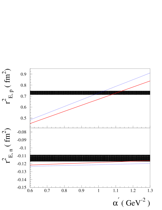
Figure 1: Proton and neutron electric mean squared radii $r^{2}_{E,p}$ (upper panel) and $r^{2}_{E,n}$ (lower panel), Eqs. (43,44). Dotted curves: Regge ansatz according to Eqs. (25,26); solid curves : modified Regge ansatz according to Eqs. (33,34). Both calculations are shown as function of the Regge slope $\alpha^{{}^{\prime}}$. For the quark distributions, the MRST02 NNLO parametrization Martin:2002dr at scale $\mu^{2}$ = 1 GeV² was used in the calculations. The shaded bands correspond to the experimental values. Note that for the neutron, the Foldy term (term proportional to $\kappa_{n}$ in Eq. (44)) gives $r^{2}_{E,n}$ = - 0.126 fm².

In Fig. 1, we show the proton and neutron rms radii as the functions of the Regge slope $\alpha^{\prime}$ for both R1 and R2 models. One notes that the neutron rms radius is dominated by the Foldy term, which gives $r^{2}_{E,n}$ = - 0.126 fm². Therefore, a relatively wide range of values $\alpha^{{}^{\prime}}$ are compatible with the neutron data. However for the proton, a rather narrow range of values around $\alpha^{{}^{\prime}}=1.0-1.1$ GeV^-2 are favored. Such value is close to the expectation from the near universal Regge slopes for meson trajectories, therefore supporting our Regge type parametrizations.

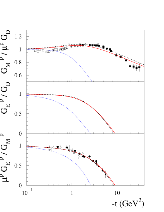
Figure 2: Proton magnetic (upper panel) and electric (middle panel) form factors relative to the dipole form $G_{D}(t)=1/(1-t/0.71)^{2}$, as well as the ratio of both form factors (lower panel). The dotted curves correspond to the Regge parametrization R1, with $\alpha^{{}^{\prime}}=1.105\,$ GeV^-2. The solid and dashed curves correspond to two fits using the modified Regge parametrization R2. The solid curves are for the 3 parameter fit : $\alpha^{{}^{\prime}}=1.105$  GeV^-2, $\eta_{u}$ = 1.713 and $\eta_{d}$ = 0.566. The dashed curves are for the 2 parameter fit : $\alpha^{{}^{\prime}}=1.09$  GeV^-2, $\eta_{u}=\eta_{d}$ = 1.34. Data for the proton magnetic form factor $G_{M}^{p}$ are from Janssens66 (open squares), Litt70 (open circles), Berger71 (solid stars), Bartel:1973rf (open stars), Andivahis:1994rq (solid circles), Sill:1992qw (solid squares), according to the recent re-analysis of Ref. Brash:2001qq . Data for the ratio $G_{E}^{p}/G_{M}^{p}$ are from Jones:1999rz (solid circles), Gayou:2001qt (open triangles), and Gayou:2001qd (solid triangles).

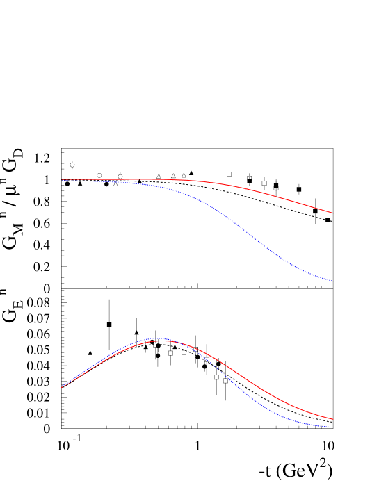
Figure 3: Neutron magnetic form factor relative to the dipole form (upper panel), and neutron electric form factor (lower panel), with curve conventions as in Fig. 2. The data for the neutron magnetic form factor $G_{M}^{n}$ are from Markowitz:hx (open circles), Xu:2000xw (solid circles), Anklin:ae (open triangels), Kubon:2001rj (solid triangles), Lung:1992bu (open squares), and Rock:1982gf (solid squares). The data for the neutron electric form factor $G_{E}^{n}$ are from different double polarization experiments at MAMI (triangles Herberg:ud ; Ostrick:xa ; Becker:tw ; Rohe:sh ), NIKHEF (solid square Passchier:1999cj ) and JLab (solid circles Zhu:2001md ; Warren:2003ma ; Madey:2003av ). The open squares are the $G_{E}^{n}$ extraction from the deuteron quadrupole form factor according to the analysis of Ref. Schiavilla:2001qe .

In Figs. 2, 3, we show the proton and neutron Sachs electric and magnetic form factors. One observes from Figs. 2, 3 that the modified Regge model R2 gives a rather good description of all available form factor data for both proton and neutron in the whole $t$ range using the parameter for the Regge trajectory $\alpha^{{}^{\prime}}$ = 1.105  GeV^-2, and the following values for the coefficients governing the $x\to 1$ behavior of the $E$-type GPDs: $\eta_{u}$ = 1.713 and $\eta_{d}$ = 0.566. The 2-parameter version of the R2 model gives a description of similar quality if we take $\alpha^{{}^{\prime}}$ = 1.09  GeV^-2 and $\eta_{u}=\eta_{d}=1.34$.
In Figs. 2 and 3, we also show the results of the initial Regge model R1, with the above value $\alpha^{{}^{\prime}}$ = 1.105  GeV^-2 of $\alpha^{\prime}$. One sees from Figs. 2, 3 that the Regge model R1 is able to reproduce the main trends of both proton and neutron electromagnetic form factor data for $-t\leq 0.5$ GeV². For higher values of $-t$, however, it falls short of the data, since as we discussed, it predicts faster power fall-off than that corresponding to the DY relation. The modified Regge model R2 reproduces the DY powers for the form factors at large $-t$, and is able to accurately describe existing data. The two additional parameters $\eta_{u}$ and $\eta_{d}$ in the R2 model, in particular, allow to describe the decreasing ratio of $G_{E}^{p}/G_{M}^{p}$ with increasing momentum transfer, as follows from the recent JLab polarization experiments Jones:1999rz ; Gayou:2001qt ; Gayou:2001qd . Our parametrization leads to a zero for $G_{E}^{p}$ at a momentum transfer of $-t\simeq 8$ GeV², which will be within the range covered by an upcoming JLab experiment E-01-109 .

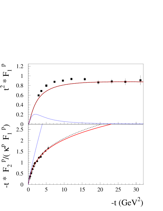
Figure 4: Proton Dirac form factor (upper panel) multiplied by $t^{2}$ and ratio of Pauli to Dirac form factor multiplied by $-t$ (lower panel), with curve conventions as in Fig. 2. The data for $F_{1}^{p}$ are from Sill:1992qw (solid squares). Data for the ratio $F_{2}^{p}/F_{1}^{p}$ are from Jones:1999rz (solid circles), Gayou:2001qt (open triangles), and Gayou:2001qd (solid triangles).

To study the large $-t$ behavior of our GPD parametrizations, it is instructive to plot the Dirac and Pauli form factors. In this way, one separates the large $-t$ behavior of both the GPDs $H$ and $E$. In Fig. 4, we show this large $-t$ behavior for $F_{1}^{p}$, and for the ratio of $F_{2}^{p}/F_{1}^{p}$. One observes from Fig. 4 that for $F_{1}^{p}$, the Regge parametrization R2 settles to an approximate $\sim 1/t^{2}$ power behavior around $-t\simeq 10$ GeV².

The ratio $F_{2}^{p}/F_{1}^{p}$ was also discussed within the context of perturbative QCD (pQCD), where the asymptotic large-$t$ behavior of the nucleon form factors is dominated by diagrams with two hard gluon exchanges Brodsky:1973kr ; Brodsky:1974vy . In any model with dimensionless quark-gluon coupling constant, these diagrams give $F_{1}^{p}\sim 1/t^{2}$  Brodsky:1973kr . Furthermore, for vector gluons, the quark helicity conservation at the gluon vertex and dimensional counting suggest the extra $m^{2}/t$ suppression for the $F_{2}^{p}$ form factor  Brodsky:1973kr ; Lepage:1979za , with $m$ being the quark mass or a nonperturbative parameter coming from the baryon wave function corresponding to extra unit of orbital angular momentum Belitsky:2002kj . Thus, one should expect that $F_{2}/F_{1}\sim 1/t$ in pQCD. Direct calculation Belitsky:2002kj , however, shows that the integrals over the quark momentum fractions $x_{i},y_{j}$ in the pQCD formula contain terms like $\varphi(x_{i},\ldots)\varphi(y_{j},\ldots)/x_{i}^{2}y_{j}^{2}$ that diverge even if the nucleon distribution amplitudes $\varphi(x_{i},\ldots),\varphi(y_{j},\ldots)$ linearly vanish at small $x_{i},y_{j}$. Strictly speaking, this means that pQCD factorization is not applicable to calculating $F_{2}^{p}(t)$ even in the asymptotic $-t\to\infty$ limit, the fact well known since the pioneering papers Lepage:1979za ; Lepage:1980fj . The authors of Ref. Belitsky:2002kj substituted the logarithmic divergences by $\log(-t/\Lambda_{QCD}^{2})$ factors, and obtained $F_{2}^{\rm pQCD}/F_{1}^{\rm pQCD}\sim\log^{2}(-t/\Lambda_{QCD}^{2})/(-t)$. This result was found to be in surprisingly good agreement with the JLab data. In this connection, we want to emphasize that our results for $F_{2}(t)$ and $F_{1}(t)$ correspond to the Feynman mechanism, i.e., to overlap of soft wave functions. The pQCD terms correspond to two iterations of the soft wave functions with hard gluon exchange kernels. As is well known, there is ${\cal O}(\alpha_{s}/\pi)$ suppression for each extra loop of a Feynman diagram in QCD. Thus, from our point of view, pQCD terms are ${\cal O}((\alpha_{s}/\pi)^{2})$ or, at most, a few per cent corrections to the Feynman mechanism contributions to $F_{1}$ and $F_{2}$. For this reason, we neglect them in our analysis. In our parametrization R2, the good description found for the ratio $F_{2}^{p}/F_{1}^{p}$ can be directly assigned to the extra suppressing factor of $(1-x)^{\eta}$ contained in the GPD $E(x,t)$. The question, how this suppression is related to the quark orbital angular momentum, deserves further investigation. It is interesting to note that the extra $(1-x)$ factor for ${\cal E}^{u}(x)$ function compared to ${\cal H}^{u}(x)$ appears in the starting term of the QCD sum rule calculation of these functions Radyushkin:2004mt . Also, the dominant $x\to 1$ perturbative QCD term for the GPD $E$ (given by $\alpha_{s}^{4}$ diagrams) involves two additional powers in $(1-x)$ compared with the pQCD expression for the leading $x\to 1$ term in the GPD $H$  Yuan:2003fs .
Since the GPD $E$ enters the sum rule for the total angular momentum $J^{q}$ carried by a quark of flavor $q$ in the proton as Ji:1996ek  :

$$2J^{q}\,=\,\int_{-1}^{1}dx\,x\,\left\{H^{q}(x,0,0)+E^{q}(x,0,0)\right\},$$ (45)

our parametrization R2, in which the $x\to 1$ limit of $E$ is determined from the $F_{2}^{p}/F_{1}^{p}$ form factor ratio, allows to evaluate the above sum rule. The first term in the sum rule of Eq. (45) is already known from the forward parton distributions and is equal to the total fraction of the proton momentum carried by a quark of flavor $q$ $(q=u,d,s)$ :

$$M_{2}^{q}\, \equiv \,\int_{-1}^{1}dx\,x\,H^{q}(x,0,0),$$ (46)

$$= \,\int_{0}^{1}dx\,x\,\left[\,q_{v}(x)+2\,\bar{q}(x)\,\right]\,,$$

with $\bar{q}(x)$ the anti-quark distribution. For the ’non-trivial’ contribution to the sum rule, arising from the second moment of the GPD $E$, we use our modified Regge parametrization R2 of Eq. (36) for ${\cal E}^{q}(x)$, which, neglecting the antiquark contribution, yields for Eq. (45) :

$$2\,J^{u}\, = \,M_{2}^{u}\,+\,\frac{\kappa^{u}}{N_{u}}\;\int_{0}^{1}dx\,x\,(1-x)^{\eta_{u}}\,u_{v}(x)\,,$$ (47)

$$2\,J^{d}\, = \,M_{2}^{d}\,+\,\frac{\kappa^{d}}{N_{d}}\;\int_{0}^{1}dx\,x\,(1-x)^{\eta_{d}}\,d_{v}(x)\,,$$ (48)

$$2\,J^{s}\, = \,M_{2}^{s}\,.$$ (49)

	$M_{2}^{q}$ (MRST2002)	$2\,J^{q}$ (R2 model)	$2\,J^{q}$ (lattice Gockeler:2003jf )
$u$	0.37	0.58	0.74 $\pm$ 0.12
$d$	0.20	-0.06	-0.08 $\pm$ 0.08
$s$	0.04	0.04
$u+d+s$	0.61	0.56	0.66 $\pm$ 0.14

Table 1: Estimate of $2\,J^{q}$ (second column) for the different quark flavors at the scale $\mu^{2}$ = 2 GeV² according to Eqs. (47-49), using the R2 parametrization (with 3 parameters) for the GPD $E$. For the forward parton distributions, the MRST2002 NNLO parametrization Martin:2002dr is used, yielding the total quark momentum contributions $M_{2}^{q}$ (first column). For comparison, the third column shows the quenched lattice QCD results of Gockeler:2003jf , extrapolated to the physical pion mass, for $2\,J^{u}$ and $2\,J^{d}$.

In Table 1, we show the values of the quark momentum sum rule $M_{2}^{q}$ at the scale $\mu^{2}$ = 2 GeV², using the MRST2002 parametrization Martin:2002dr for the forward parton distributions. We also show the estimate for $J^{u}$, $J^{d}$, and $J^{s}$ of Eqs. (47-49) at the same scale. As was already observed in Ref. Goeke:2001tz , based on a Regge model of the type R1, our estimates lead to a large fraction (63 %) of the total angular momentum of the proton carried by the $u$-quarks and a relatively small contribution carried by the $d$-quarks. As the $d$-quark intrinsic spin contribution is known to be relatively large and negative ( $\Delta d_{v}\simeq-0.25$ ), the small total angular momentum contribution $J^{d}$ of the $d$-quarks which follows from our parametrization implies an interesting cancellation between the intrinsic spin contribution and the orbital contribution $L^{d}$ ( with $2J^{q}=\Delta q+2L^{q}$ ), which should therefore be of size $2L^{d}\simeq 0.2$. For the $u$-quark on the other hand, the parametrization R2 yields only a small value for $2L^{u}$, as our estimate for $2J^{u}$ is quite close to the intrinsic spin contribution $\Delta u_{v}\simeq 0.6$. Such a picture is also supported by a recent quenched lattice QCD calculation Gockeler:2003jf (see also Mathur:1999uf for an earlier calculation) for the valence quark contributions to $2J^{u}$ and $2J^{d}$. One indeed sees from Table 1 (third column) that the quenched lattice QCD calculation yields quite similar values for $2J^{u}$ and $2J^{d}$ as our parametrization R2. It remains to be seen however how large is the sea quark contribution to the GPD $E$ which can enter the spin sum rule of Eq. (45). This sea quark contribution is only approximately included (i.e. fermion loop contributions are neglected) in the quenched lattice QCD calculations of Ref. Gockeler:2003jf . An exploratory investigation using unquenched QCD configurations has been performed in Ref. Hagler:2003jd . The sea quark contribution is also not constrained by the form factor sum rules considered in this paper, which only constrain the valence quark distributions. Ongoing measurements of hard exclusive processes, such as deeply virtual Compton scattering, provide a means to address this question in the near future.

Besides the electromagnetic form factors for proton and neutron, the Regge parametrizations discussed in this work can also be used to estimate $N\to\Delta$ transition form factors, provided one can relate the $N\to\Delta$ transition GPDs to the $N\to N$ ones. First experiments which are sensitive to the $N\to\Delta$ GPDs have recently been reported Guidal:2003ji . For the magnetic $N\to\Delta$ transition form factor $G_{M}^{*}(t)$, it was shown in Ref. Frankfurt:1999xe that, in the large $N_{c}$ limit, the relevant $N\to\Delta$ GPD can be expressed in terms of the isovector GPD $E^{u}-E^{d}$, yielding the sum rule

$$G_{M}^{*}(t)\,=\,{{G_{M}^{*}(0)}\over{\kappa_{V}}}\;\int_{-1}^{+1}dx\;\biggl{\{}E^{u}(x,\xi,t)\,-\,E^{d}(x,\xi,t)\biggr{\}}\;=\;{{G_{M}^{*}(0)}\over{\kappa_{V}}}\;\biggl{\{}F_{2}^{p}(t)-F_{2}^{n}(t)\biggr{\}}\,,$$ (50)

where $\kappa_{V}=\kappa_{p}-\kappa_{n}=3.70$. Within the large $N_{c}$ approach used in Ref. Frankfurt:1999xe , the value $G_{M}^{*}(0)$ is given by $G_{M}^{*}(0)=\kappa_{V}/\sqrt{3}$ Goeke:2001tz , which is about 30% smaller than the experimental number. In our calculations, we will therefore use the phenomenological value $G_{M}^{*}(0)\approx 3.02$ Tiator:2000iy .

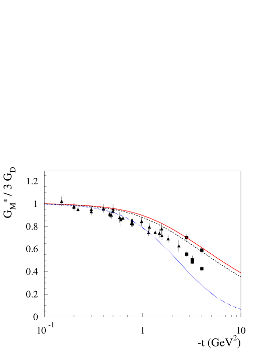
Figure 5: The $N\to\Delta$ magnetic transition form factor, relative to the dipole form (multiplied by a factor 3). Curve conventions as in Fig. 2. The data for $G_{M}^{*}$ are from the compilation of Tiator:2000iy . For the JLab data points at 2.8 and 4 GeV², both the analyses of Frolov:1998pw (upper points) and Tiator:2000iy (lower points) are shown.

We show our results for $G_{M}^{*}$ using Eq. (50) in Fig. 5. It is seen that both the Regge and modified Regge parametrizations yield a magnetic $N\to\Delta$ form factor which decreases faster than a dipole, in qualitative good agreement with the data.

The sum rule (50) was used earlier by P. Stoler Stoler:2002im , who proposed a model Stoler:2001xa ; Stoler:2003mx in which the Gaussian ansatz for GPDs is modified at large $-t$ by terms having a power-law behavior.

VII GPDs in impact parameter space and positivity constraints

The models for GPDs should satisfy many constraints. In fact, such constraints as the reduction of GPDs to usual parton densities in the forward limit and to form factors in the local limit, are the key points for the models constructed in this paper. There are more complicated constraints imposed, e.g., by the polynomiality condition which is extremely important for nonzero skewness. Since the nonforward parton densities correspond to $\xi=0$, they are not affected by these constraints. However, they are affected by the positivity conditions which should be taken into account both for nonzero and zero skewness parameter. In particular, there exists a relation between the $E$-type and $H$-type GPDs Burkardt:2003ck . Since we are constructing $E$-GPDs from $H$-GPDs by a simple modification of the $x$-behavior of $H$ by a power of $(1-x)$, we should check that such a modification is consistent with the positivity constraint of Ref. Burkardt:2003ck .

The most convenient formulation of the positivity constraint relating the $E$ and $H$ GPDs is in the impact parameter space. For $\xi=0$, the impact parameter versions of GPDs are obtained through a Fourier integral in transverse momentum $q_{\perp}$ :

$$H^{q}(x,{\bf b_{\perp}})\, \equiv \,\int\frac{d^{2}{\bf q_{\perp}}}{(2\pi)^{2}}\,e^{i{\bf b_{\perp}\cdot q_{\perp}}}\;{\cal H}^{q}(x,-{\bf q_{\perp}^{2}}),$$ (51)

$$E^{q}(x,{\bf b_{\perp}})\, \equiv \,\int\frac{d^{2}{\bf q_{\perp}}}{(2\pi)^{2}}\,e^{i{\bf b_{\perp}\cdot q_{\perp}}}\;{\cal E}^{q}(x,-{\bf q_{\perp}^{2}}),$$ (52)

These functions have the physical meaning of measuring the probability to find a quark which carries longitudinal momentum fraction $x$ at a transverse position ${\bf b_{\perp}}$ in a nucleon, see Refs. Burkardt:2000za ; Burkardt:2002hr .

It has been shown Burkardt:2003ck that the GPDs $H$ and $E$ in the impact parameter space satisfy the positivity bound :

$$\frac{1}{2M_{N}}\,\left|{\bf\nabla_{b_{\perp}}}\,E^{q}(x,{\bf b_{\perp}})\right|\, \leq \,H^{q}(x,{\bf b_{\perp}}).$$ (53)

Translating the GPD parametrization R2 of Eqs. (29,35), into the impact parameter space, we obtain :

$$H^{q}(x,{\bf b_{\perp}})\, = \,q_{v}(x)\,\frac{e^{-{\bf b_{\perp}}^{2}\,/\,[-4\,\alpha^{\,{}^{\prime}}\,(1-x)\ln x]}}{4\pi\,\left[-\alpha^{\,{}^{\prime}}(1-x)\ln x\right]},$$ (54)

$$E^{q}(x,{\bf b_{\perp}})\, = \,\frac{\kappa_{q}}{N_{q}}\,(1-x)^{\eta_{q}}\,q_{v}(x)\,\frac{e^{-{\bf b_{\perp}}^{2}\,/\,[-4\,\alpha^{\,{}^{\prime}}\,(1-x)\ln x]}}{4\pi\,\left[-\alpha^{\,{}^{\prime}}(1-x)\ln x\right]},$$ (55)

from which it follows that

$$\left|{\bf\nabla_{b_{\perp}}}\,E^{q}(x,{\bf b_{\perp}})\right|\,=\,\frac{\kappa_{q}}{N_{q}}\,(1-x)^{\eta_{q}}\,q_{v}(x)\,\frac{\left|\bf{b_{\perp}}\right|}{2}\,\frac{e^{-{\bf b_{\perp}}^{2}\,/\,[-4\,\alpha^{\,{}^{\prime}}\,(1-x)\ln x]}}{4\pi\,\left[-\alpha^{\,{}^{\prime}}(1-x)\ln x\right]^{2}},$$ (56)

Within the R2 parametrization, the positivity bound of Eq. (53) implies an upper bound on the value of $\left|\bf{b_{\perp}}\right|$ :

$$\left|\bf{b_{\perp}}\right|\,\leq\,\frac{N_{q}}{\left|\kappa_{q}\right|}\,\frac{M_{N}}{(1-x)^{\eta_{q}}}\,4\,\left[-\alpha^{\,{}^{\prime}}(1-x)\ln x\right].$$ (57)

In Fig. 6, we show the GPDs in the impact parameter space for the modified Regge parametrization R2 discussed above. The parameters are taken from the best fit to the form factors as discussed in the previous section. We see from Fig. 6 that for the $u$-quark GPDs, the positivity bound of Eq. (53) is satisfied over most of the $x$-region, considering that the GPDs are vanishingly small for values of ${\bf b_{\perp}}$ larger than the nucleon size (corresponding with about 4.4 GeV^-1). For the $d$-quark GPDs on the other hand, there is a violation in the present parametrization, which becomes more pronounced at larger values of $x$ and ${\bf b_{\perp}}$, as is shown in Fig. 7 (left panel). We therefore tried to extend the range of validity of the R2 parametrization by finding a fit with a higher value of $\eta_{d}$. This can be obtained by imposing the constraint $\eta_{u}=\eta_{d}$. We have shown before that the resulting two-parameter fit ($\alpha^{{}^{\prime}}=1.09$  GeV^-2, $\eta_{u}=\eta_{d}$ = 1.34) gives a nearly as satisfactory description of the form factors. It is seen from the right panel in Fig. 7 that this 2-parameter fit extends the region in $x$ and ${\bf b_{\perp}}$ for the d-quark where our parametrization satisfies the positivity condition.

It is clear, that with a somewhat more complicated model, we can easily satisfy the positivity constraint. However, given that the violation is rather small, we prefer not to introduce extra parameters and to keep the parametrization as simple as possible.

Furthermore, it is clearly seen from these images that for large values of $x$, our quark distributions are concentrated at small values of ${\bf b_{\perp}}$, reflecting the distribution of valence quarks in the core of the nucleon. On the other hand, at small values of $x$, the distribution in transverse position extends much further out. This expected correlation assures that our model correctly reproduces the gross features of the nucleon structure as expressed in terms of the quark distributions.

Figure 6: GPDs in impact parameter space for the modified Regge parametrization R2, with parameters $\alpha^{{}^{\prime}}=1.105$  GeV^-2, $\eta_{u}$ = 1.713 and $\eta_{d}$ = 0.566. Left panels for $u$-quark; right panels for $d$-quark. The solid (dashed) curves give GPDs $H^{q}$ ($E^{q}$), respectively. The dotted curves correspond to the function $\left|{\bf\nabla_{b_{\perp}}}\,E^{q}\right|/(2M_{N})$ entering the positivity bound of Eq. (53).

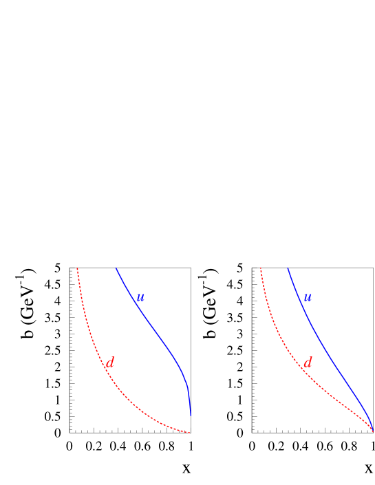
Figure 7: Upper bound on ${\bf b_{\perp}}$ ( Eq. (57) ) required by the positivity bound of Eq. (53) for two fits using the Regge parametrization R2. Left panel is for the 3 parameter fit : $\alpha^{{}^{\prime}}=1.105$  GeV^-2, $\eta_{u}$ = 1.713 and $\eta_{d}$ = 0.566. Right panel is for the 2 parameter fit : $\alpha^{{}^{\prime}}=1.09$  GeV^-2, $\eta_{u}=\eta_{d}$ = 1.34.

VIII Conclusions

Summarizing, we discussed in this work several parametrizations for the $t$-dependence of the nucleon GPDs in view of the recent accurate data for the nucleon electromagnetic form factors in the spacelike region.
Starting from the low $-t$ region, we discussed a Regge model in which the $x$ and $t$ dependence of the GPDs are coupled in the form $x^{-\alpha^{\prime}\,t}$. This model has only one parameter which physically corresponds to the slope $\alpha^{\prime}$ of the Regge trajectory in the vector EM current channel. This parameter is linearly related to the rms radii of $F_{1}$ and $F_{2}$ form factors, and it was found that both radii are well deccribed by the same universal Regge slope.
Such a Regge model leads however to faster power fall-off of form factors in the large $-t$ region than that expected from the Drell-Yan relation. To conform with this relation and the observed power behavior at large $-t$, we used a modified Regge parametrization that gives slower decrease with $-t$. The modified Regge parametrization displays approximately a $1/t^{2}$ behavior for $F_{1}^{p}(t)$ data in the region $-t\geq 10$ GeV². To describe $F_{2}^{p}(t)$, we need to introduce, in addition to $\alpha^{\prime}$, two parameters that govern the $x\to 1$ behavior of the GPD $E$. They were adjusted to give an accurate description of the recent polarization data for the ratio $F_{2}^{p}/F_{1}^{p}$. Since this behavior in our model is correlated with the $x\to 1$ behavior of the GPD $E$, it also allows us to evaluate the sum rule for the total angular momentum carried by the quarks, which involves the second moment of the GPD $E$.
For the quark contributions to the nucleon spin, we find an intriguing flavor dependence, in which the valence $u$-quark contributes about two-thirds of the proton’s spin (at a low renormalization point), which is nearly entirely arising from the $u$-quarks intrinsic spin contribution. For the valence $d$-quark on the other hand, our parametrization implies a near cancellation between its negative intrinsic spin contribution and its orbital angular momentum contribution. Recent quenched lattice QCD calculations support this observation.
It remains to be seen by how much the sea quarks affect this picture. Ongoing measurements of hard exclusive processes, such as deeply virtual Compton scattering, are a means to address this question. As the GPDs mostly enter in hard exclusive observables through convolution integrals, our parametrization, which builds in the constraint coming from the first moment through the nucleon electromagnetic form factors, can be used as a first step to unravel the information on GPDs from the observables. The present work also suggests several interesting directions for future research. One of them is the extension of this study to quantify the link between the nucleon strangeness form factors and the $s$-quark distributions. Furthermore, the study of the chiral corrections (pion mass dependence) to the GPDs will allow to match onto the corresponding known chiral behavior of the elastic form factors at small momentum transfer.

References

- (1) D. Muller, D. Robaschik, B. Geyer, F. M. Dittes and J. Horejsi, Fortsch. Phys. 42, 101 (1994).
- (2) X. D. Ji, Phys. Rev. Lett. 78, 610 (1997), Phys. Rev. D 55, 7114 (1997).
- (3) A. V. Radyushkin, Phys. Rev. D 56, 5524 (1997).
- (4) X. D. Ji, J. Phys. G 24, 1181 (1998) [arXiv:hep-ph/9807358].
- (5) A. V. Radyushkin, in “At the Frontier of Particle Physics / Handbook of QCD”, edited by M. Shifman (World Scientific, Singapore, 2001), vol. 2, pp. 1037-1099; arXiv:hep-ph/0101225.
- (6) K. Goeke, M. V. Polyakov and M. Vanderhaeghen, Prog. Part. Nucl. Phys. 47, 401 (2001) [arXiv:hep-ph/0106012].
- (7) M. Diehl, Phys. Rept. 388, 41 (2003) [arXiv:hep-ph/0307382].
- (8) A. V. Belitsky and A. V. Radyushkin, arXiv:hep-ph/0504030.
- (9) M. Burkardt, Phys. Rev. D 62, 071503 (2000) [Erratum-ibid. D 66, 119903 (2002)] [arXiv:hep-ph/0005108].
- (10) M. Burkardt, Int. J. Mod. Phys. A 18, 173 (2003) [arXiv:hep-ph/0207047].
- (11) M. Diehl, Eur. Phys. J. C 25, 223 (2002) [Erratum-ibid. C 31, 277 (2003)] [arXiv:hep-ph/0205208].
- (12) J. P. Ralston and B. Pire, Phys. Rev. D 66, 111501 (2002) [arXiv:hep-ph/0110075].
- (13) A. V. Belitsky, X. D. Ji and F. Yuan, Phys. Rev. D 69, 074014 (2004) [arXiv:hep-ph/0307383].
- (14) LHPC, P. Hagler, J. W. Negele, D. B. Renner, W. Schroers, T. Lippert and K. Schilling [LHPC Collaboration], arXiv:hep-lat/0312014.
- (15) A. V. Radyushkin, Phys. Rev. D 58, 114008 (1998) [arXiv:hep-ph/9803316].
- (16) M. Diehl, T. Feldmann, R. Jakob and P. Kroll, Eur. Phys. J. C 8, 409 (1999).
- (17) A. V. Afanasev, arXiv:hep-ph/9910565.
- (18) P. Stoler, Phys. Rev. D 65, 053013 (2002) [arXiv:hep-ph/0108257].
- (19) P. Stoler, arXiv:hep-ph/0307162.
- (20) M. Diehl, T. Feldmann, R. Jakob and P. Kroll, Eur. Phys. J. C 39, 1 (2005) [arXiv:hep-ph/0408173].
- (21) M. Vanderhaeghen, in: “Proceedings of the Workshop on Exclusive Processes at High Momentum Transfer, Newport News, Virginia, 15-18 May 2002”, edited by A. Radyushkin and P. Stoler (World Scientific, Singapore, 2002), p.51.
- (22) A. V. Radyushkin, in: “Continuous Advances in QCD 2004”, edited by T. Ghergetta (World Scientific, Singapore, 2004), pp. 3-14, [arXiv:hep-ph/0409215].
- (23) S. D. Drell and T. M. Yan, Phys. Rev. Lett. 24, 181 (1970).
- (24) V. Barone, M. Genovese, N. N. Nikolaev, E. Predazzi and B. G. Zakharov, Z. Phys. C 58, 541 (1993).
- (25) G. B. West, Phys. Rev. Lett. 24, 1206 (1970).
- (26) M. Burkardt, Phys. Lett. B 595, 245 (2004) [arXiv:hep-ph/0401159].
- (27) E. D. Bloom and F. J. Gilman, Phys. Rev. Lett. 25, 1140 (1970).
- (28) G. P. Lepage and S. J. Brodsky, Phys. Rev. D 22, 2157 (1980).
- (29) A. D. Martin, R. G. Roberts, W. J. Stirling and R. S. Thorne, Phys. Lett. B 531, 216 (2002) [arXiv:hep-ph/0201127].
- (30) M. Burkardt, Phys. Lett. B 582, 151 (2004) [arXiv:hep-ph/0309116].
- (31) T. Janssens et al., Phys. Rev. 142, 922 (1966).
- (32) J. Litt et al., Phys. Lett. B 31, 40 (1970).
- (33) Ch. Berger et al., Phys. Lett. B 35, 87 (1971).
- (34) W. Bartel et al., Nucl. Phys. B 58, 429 (1973).
- (35) L. Andivahis et al., Phys. Rev. D 50, 5491 (1994).
- (36) A. F. Sill et al., Phys. Rev. D 48, 29 (1993).
- (37) E. J. Brash, A. Kozlov, S. Li and G. M. Huber, Phys. Rev. C 65, 051001 (2002) [arXiv:hep-ex/0111038].
- (38) M. K. Jones et al. [Jefferson Lab Hall A Collaboration], Phys. Rev. Lett. 84, 1398 (2000) [arXiv:nucl-ex/9910005].
- (39) O. Gayou et al., Phys. Rev. C 64, 038202 (2001).
- (40) O. Gayou et al. [Jefferson Lab Hall A Collaboration], Phys. Rev. Lett. 88, 092301 (2002) [arXiv:nucl-ex/0111010].
- (41) P. Markowitz et al., Phys. Rev. C 48, 5 (1993).
- (42) W. Xu et al., Phys. Rev. Lett. 85, 2900 (2000) [arXiv:nucl-ex/0008003].
- (43) H. Anklin et al., Phys. Lett. B 428, 248 (1998).
- (44) G. Kubon et al., Phys. Lett. B 524, 26 (2002) [arXiv:nucl-ex/0107016].
- (45) A. Lung et al., Phys. Rev. Lett. 70, 718 (1993).
- (46) S. Rock et al., Phys. Rev. Lett. 49, 1139 (1982).
- (47) C. Herberg et al., Eur. Phys. J. A 5, 131 (1999).
- (48) M. Ostrick et al., Phys. Rev. Lett. 83, 276 (1999).
- (49) J. Becker et al., Eur. Phys. J. A 6, 329 (1999).
- (50) D. Rohe et al., Phys. Rev. Lett. 83, 4257 (1999).
- (51) I. Passchier et al., Phys. Rev. Lett. 82, 4988 (1999) [arXiv:nucl-ex/9907012].
- (52) H. Zhu et al. [E93026 Collaboration], Phys. Rev. Lett. 87, 081801 (2001) [arXiv:nucl-ex/0105001].
- (53) G. Warren et al. [Jefferson Lab E93-026 Collaboration], Phys. Rev. Lett. 92, 042301 (2004) [arXiv:nucl-ex/0308021].
- (54) R. Madey et al. [E93-038 Collaboration], Phys. Rev. Lett. 91, 122002 (2003) [arXiv:nucl-ex/0308007].
- (55) R. Schiavilla and I. Sick, Phys. Rev. C 64, 041002 (2001) [arXiv:nucl-ex/0107004].
- (56) JLab experiment E-01-109 / E-04-108, spokespersons : E. Brash, M. Jones, C. Perdrisat, V. Punjabi.
- (57) S. J. Brodsky and G. R. Farrar, Phys. Rev. Lett. 31, 1153 (1973).
- (58) S. J. Brodsky and G. R. Farrar, Phys. Rev. D 11, 1309 (1975).
- (59) G. P. Lepage and S. J. Brodsky, Phys. Rev. Lett. 43, 545 (1979) [Erratum-ibid. 43, 1625 (1979)].
- (60) A. V. Belitsky, X. d. Ji and F. Yuan, Phys. Rev. Lett. 91, 092003 (2003) [arXiv:hep-ph/0212351].
- (61) A. Radyushkin, Annalen Phys. 13, 718 (2004) [arXiv:hep-ph/0410153].
- (62) F. Yuan, Phys. Rev. D 69, 051501 (2004) [arXiv:hep-ph/0311288].
- (63) M. Gockeler, R. Horsley, D. Pleiter, P. E. L. Rakow, A. Schafer, G. Schierholz and W. Schroers [QCDSF Collaboration], Phys. Rev. Lett. 92, 042002 (2004) [arXiv:hep-ph/0304249].
- (64) N. Mathur, S. J. Dong, K. F. Liu, L. Mankiewicz and N. C. Mukhopadhyay, Phys. Rev. D 62, 114504 (2000) [arXiv:hep-ph/9912289].
- (65) P. Hagler, J. Negele, D. B. Renner, W. Schroers, T. Lippert and K. Schilling [LHPC collaboration], Phys. Rev. D 68, 034505 (2003) [arXiv:hep-lat/0304018].
- (66) M. Guidal, S. Bouchigny, J. P. Didelez, C. Hadjidakis, E. Hourany and M. Vanderhaeghen, Nucl. Phys. A 721, 327 (2003) [arXiv:hep-ph/0304252].
- (67) L. L. Frankfurt, M. V. Polyakov, M. Strikman and M. Vanderhaeghen, Phys. Rev. Lett. 84, 2589 (2000) [arXiv:hep-ph/9911381].
- (68) P. Stoler, Phys. Rev. Lett. 91, 172303 (2003) [arXiv:hep-ph/0210184].
- (69) L. Tiator, D. Drechsel, O. Hanstein, S. S. Kamalov and S. N. Yang, Nucl. Phys. A 689, 205 (2001) [arXiv:nucl-th/0012046].
- (70) V. V. Frolov et al., Phys. Rev. Lett. 82, 45 (1999) [arXiv:hep-ex/9808024].