DESY 04-194 Edinburgh 2004/24 LTH 638 LU-ITP 2004/039 October 2004 A lattice determination of moments of unpolarised nucleon structure functions using improved Wilson fermions

Abstract

Within the framework of quenched lattice QCD and using $O(a)$ improved Wilson fermions and non-perturbative renormalisation, a high statistics computation of low moments of the unpolarised nucleon structure functions is given. Particular attention is paid to the chiral and continuum extrapolations.

1 Introduction

The results of a lattice simulation of Quantum Chromodynamics (QCD) give in principle a direct probe of certain low energy aspects of the theory, such as hadronic masses and matrix elements. This is at present the only way of getting these quantities from QCD, without additional model-dependent assumptions. A useful theoretical tool in conjunction with QCD and deep inelastic scattering (or DIS) experiments is the operator product expansion, OPE. At leading twist the OPE relates moments of an experimentally measured structure function, generically denoted by $F$, to certain matrix elements $v_{n}$ where

$$\int_{0}^{1}dxx^{n-2}F^{\mbox{\tiny$N\!S$}}(x,Q^{2})=fE_{F;v_{n}}^{\cal S}\left({M^{2}\over Q^{2}},g^{\cal S}(M)\right)v_{n}^{\cal S}(g^{\cal S}(M))\,.$$ (1)

$F$ is a function of two variables – $Q^{2}$, the space-like momentum transfer to the nucleon and $x$, the Bjorken variable ($f$ is a normalisation factor). $v_{n}$ are the nucleon matrix elements of certain operators and $E$ are the associated Wilson coefficients. These are perturbatively known at high energies where the coupling constant $g$ becomes small and are found in a specified scheme ${\cal S}$ at scale $M$. Usually, of course, we take ${\cal S}\equiv\overline{MS}$ at scale $M\equiv\mu\sim$ few GeV. We also assume that $Q^{2}$ is large enough, so that higher twist terms ie $O(1/Q^{2})$ terms are negligible.

As will be discussed later (section 4.3), lattice computations are presently restricted to determining non-singlet, NS, nucleon structure functions

$$F^{\mbox{\tiny$N\!S$}}(x,Q^{2})\equiv F^{p}(x,Q^{2})-F^{n}(x,Q^{2})\,,$$ (2)

ie the difference between proton, $p$, and neutron, $n$, results. Note in particular that this means that nucleon matrix elements of gluonic operators have cancelled.

In this article we shall only be concerned with unpolarised structure functions. The same matrix elements $v_{n}$ contribute to the scattering of charged leptons and of neutrinos, but the weights $f$ are different in the two cases. Thus for charged lepton–nucleon DIS, $lN\to lX$, which is mediated by a photon, we have $F^{\mbox{\tiny$N\!S$}}\to F_{2}^{\gamma;\mbox{\tiny$N\!S$}}$ with $n=2,4,\ldots$ and $f^{\gamma}=2(e_{u}^{2}-e_{d}^{2})/2=1/3$. For neutrino–nucleon charged weak current interactions for example $\nu N\to lX$, ($l^{+}N\to\overline{\nu}X$) or $lN\to\nu X$, ($\overline{\nu}N\to l^{+}X$) which are mediated by $W^{+}$, $W^{-}$ respectively, then we have $F^{\mbox{\tiny$N\!S$}}\to F_{2}^{W^{\pm};\mbox{\tiny$N\!S$}}$ and $f^{W^{+}}=2(-1)$, $f^{W^{-}}=2(+1)$ (neglecting the CKM mixing matrix) with $n=3,5,\ldots$. (Alternatively setting $F^{\mbox{\tiny$N\!S$}}\to 2xF_{1}^{\mbox{\tiny$N\!S$}}$ in all cases one has the same matrix elements and $f$s as for $F_{2}^{\mbox{\tiny$N\!S$}}$ in eq. (1), but different Wilson coefficients. The additional $F_{3}$ structure functions, occuring because of parity non-conservation also obey eq. (1) with $F^{\mbox{\tiny$N\!S$}}\to xF_{3}^{W^{\pm};\mbox{\tiny$N\!S$}}$ and again $f^{W^{\pm}}=\mp 2$ with $n=2,4,\ldots$.) Similar expressions hold for the neutral currents, but with more complicated expressions for the $f$s.

In all cases the relevant matrix elements are given by first defining the sequence of quark bilinear forms

$${\cal O}^{\mu_{1}\cdots\mu_{n}}_{q} = i^{n-1}\overline{q}\gamma^{\mu_{1}}\stackrel{{\scriptstyle\leftrightarrow}}{{{D}^{\mu_{2}}}}\cdots\stackrel{{\scriptstyle\leftrightarrow}}{{{D}^{\mu_{n}}}}q,\qquad q=u,d\,,$$ (3)

where $\stackrel{{\scriptstyle\leftrightarrow}}{{D}}=\mbox{\small$\frac{1}{2}$}(\stackrel{{\scriptstyle\rightarrow}}{{D}}-\stackrel{{\scriptstyle\leftarrow}}{{D}})$. Symmetrising the indices and removing traces, gives the Lorentz decomposition of the proton (ie nucleon, N) matrix element of

$$\langle N(\vec{p}\,)|\left[{\cal O}^{\{\mu_{1}\cdots\mu_{n}\}}_{q}-\mbox{\rm Tr}\right]|N(\vec{p}\,)\rangle^{\cal S}\equiv 2v^{(q){\cal S}}_{n}[p^{\mu_{1}}\cdots p^{\mu_{n}}-\mbox{\rm Tr}]\,.$$ (4)

For example we have for $n=2$,

$$\langle N(\vec{p}\,)|i\overline{q}\left[\mbox{\small$\frac{1}{2}$}[\gamma^{\mu_{1}}\stackrel{{\scriptstyle\leftrightarrow}}{{{D}^{\mu_{2}}}}+\gamma^{\mu_{2}}\stackrel{{\scriptstyle\leftrightarrow}}{{{D}^{\mu_{1}}}}]-\mbox{\small$\frac{1}{4}$}\stackrel{{\scriptstyle\leftrightarrow}}{{\not{D}}}\eta^{\mu_{1}\mu_{2}}\right]q|N(\vec{p}\,)\rangle^{\cal S}$$ (5)

$$= 2v^{(q){\cal S}}_{2}\left[p^{\mu_{1}}p^{\mu_{2}}-\mbox{\small$\frac{1}{4}$}m_{N}^{2}\eta^{\mu_{1}\mu_{2}}\right]\,,$$

and more complicated expressions hold for higher moments. Finally, the non-singlet, NS, matrix element is defined as

$$v^{\cal S}_{n}\equiv v^{(u){\cal S}}_{n}-v^{(d){\cal S}}_{n}\,.$$ (6)

In this article, we shall compute $v_{2}$, $v_{3}$ and $v_{4}$ in the quenched approximation ($n_{f}=0$), by finding the appropriate matrix elements in eq. (4). As will be seen most effort will be spent on $v_{2}$, as this is technically less complicated than the higher moments, and also numerically the lattice results are more precise. The lattice approach discretises Euclidean space-time, with lattice spacing $a$, in the path integral and simulates the resulting high-dimensional integral for the partition function using Monte Carlo techniques. Matrix elements can then be obtained from suitable ratios of correlation functions, [1, 2]. Note that the lattice programme is rather like an experiment: careful account must be taken of error estimations and extrapolations. There are three limits to consider:

• The spatial box size $L_{S}$ must be large enough so that finite size effects are small. Currently sizes of $\mathrel{\hbox to0.0pt{\lower 4.0pt\hbox{\hskip 1.0pt$\sim$}\hss}\raise 1.0pt\hbox{$>$}}2\,\mbox{fm}$ seem large enough (the nucleon diameter is about $1.5\,\mbox{fm}$). This situation is probably more favourable for quenched QCD (where one drops the fermion determinant in the path integral, see section 4), as due to the suppression of the pion cloud, we would expect the radius of the nucleon to be somewhat smaller. This indeed seems to be the case, see eg [3].

• The continuum limit, $a\to 0$. We use $O(a)$ improved Wilson fermions (where the discretisation effects of the action and matrix elements have been arranged to be $O(a^{2})$). For unimproved Wilson fermions, or where one has not succeeded in entirely $O(a)$ improving the matrix element we should extrapolate in $a$ rather than $a^{2}$.

• The chiral limit, when the quark mass approaches zero. There has recently been much activity on deriving formulae for this limit, [4, 5, 6, 7, 8, 9]. However while most of these results are valid around the physical pion mass on the lattice, it is difficult to calculate quark propagators at quark masses much below the strange quark mass. Thus the use of these formulae is not straightforward.

In addition the lattice matrix element must also be renormalised.

Previous lattice studies gave discrepancies to the phenomenological results, especially for $v_{2}$. In this work we want to try to narrow down the sources for this difference. In particular we shall present here non-perturbative, NP, results for the renormalisation constants (and as many previous studies used results based on perturbation theory compare with these other results). We also consider $O(a)$ improvement and operator mixing to enable a reliable continuum extrapolation to be performed.

Compared to our previous work [2] we have improved our techniques in several respects:

• We employ non-perturbatively improved Wilson fermions instead of unimproved Wilson fermions. This should reduce cut-off effects.

• Modified operators are used for $v_{3}$, $v_{4}$, which improves the numerical signal.

• In [2] we had simulations for a single lattice spacing only. Here we shall present results for three different values of the lattice spacing so that we can monitor lattice artefacts.

• As mentioned before, the 1-loop perturbative renormalisation factors of [2] have been replaced by non-perturbatively calculated renormalisation constants. In addition we shall pay close attention to possible mixing problems of the operators involved.

• We have increased the number of quark masses at each value of the lattice spacing in order to improve the chiral extrapolation.

The organisation of this paper is as follows. In section 2 various continuum results for the $\beta$ and $\gamma$ functions and for the Wilson coefficients in the $\overline{MS}$ scheme are collated and renormalisation group invariant quantities are introduced, while in section 3 some NS phenomenological results are discussed to compare later with the lattice results. Section 4 describes our lattice techniques: choice of operators, operator mixing problems, $O(a)$ improvement and gives the bare, ie unrenormalised results. Section 5 discusses and compares various renormalisation results: one-loop perturbation theory and a tadpole improvement, together with the $\rm{RI}^{\prime}-\rm{MOM}$ non-perturbative method. In section 6 we discuss the results and give continuum and chiral extrapolations. Finally in section 7 we present our conclusions.

2 Continuum QCD results

In this section we shall consider the RHS of eq. (1). Much of the functional form is already known: the lattice input is reduced to the computation of a single number (for each moment).

The running of the coupling constant as the scale $M$ is changed is controlled by the $\beta$ function. This is defined as

$$\beta^{\cal S}\left(g^{\cal S}(M)\right) \equiv \left.{\partial g^{\cal S}(M)\over\partial\log M}\right|_{bare}$$ (7)

$$= -b_{0}(g^{\cal S})^{3}-b_{1}(g^{\cal S})^{5}-b_{2}^{\cal S}(g^{\cal S})^{7}-b_{3}^{\cal S}(g^{\cal S})^{9}-\ldots\,,$$

with the bare parameters being held constant. This function is given perturbatively as a power series expansion in the coupling constant. The first two coefficients in the expansion are universal (ie scheme independent). In the $\overline{MS}$ scheme where $({\cal S},M)=(\overline{MS},\mu)$, the expansion is now known to four loops [10, 11]. The three-loop result for quenched QCD is

$$b_{0}={11\over(4\pi)^{2}}\,,\qquad b_{1}={102\over(4\pi)^{4}}\,,\qquad b_{2}^{\mbox{\tiny$\overline{MS}$}}={1\over(4\pi)^{6}}\left[{2857\over 2}\right]\,.$$ (8)

We may immediately integrate eq. (7) to obtain the solution,

$$M=\Lambda^{\cal S}\exp{\left[{1\over 2b_{0}g^{\cal S}(M)^{2}}\right]}\left[b_{0}g^{\cal S}(M)^{2}\right]^{b_{1}\over 2b_{0}^{2}}\exp{\left\{\int_{0}^{g^{\cal S}(M)}\!\!d\xi\left[{1\over\beta^{\cal S}(\xi)}+{1\over b_{0}\xi^{3}}-{b_{1}\over b_{0}^{2}\xi}\right]\right\}}\,,$$ (9)

where $\Lambda^{\cal S}$ is an integration constant.

While eq. (1) is the conventional definition of the moment of a structure function, for us it is more convenient to re-write it using renormalisation group invariant (or RGI) functions. The bare operator (or matrix element) must first be renormalised

$${\cal O}^{\cal S}(M)=Z_{{\cal O};bare}^{\phantom{{\cal O};}{\cal S}}(M){\cal O}_{bare}\,,$$ (10)

giving $\gamma$, the anomalous dimension of the operator,

$$\gamma^{\cal S}_{\cal O}\left(g^{\cal S}(M)\right) \equiv \left.{\partial\log Z_{{\cal O}}^{\phantom{{\cal O}}\cal S}(M)\over\partial\log M}\right|_{bare}$$ (11)

$$= d_{{\cal O};0}(g^{\cal S})^{2}+d_{{\cal O};1}^{\cal S}(g^{\cal S})^{4}+d_{{\cal O};2}^{\cal S}(g^{\cal S})^{6}+\ldots\,.$$

(The first coefficient is again scheme independent.) One may also change the scale and/or scheme $({\cal S},M)\to({\cal S}^{\prime},M^{\prime})$ for the operator by

$${\cal O}^{{\cal S}^{\prime}}(M^{\prime})=Z_{{\cal O};{\cal S}}^{\phantom{{\cal O},}{\cal S}^{\prime}}(M^{\prime},M){\cal O}^{\cal S}(M)\,.$$ (12)

This leads to two anomalous dimension equations, obtained by either differentiating with respect to $M^{\prime}$ or $M$. Integrating these equations gives

$$Z_{{\cal O};{\cal S}}^{\phantom{{\cal O};}{\cal S}^{\prime}}(M^{\prime},M)={Z_{{\cal O};bare}^{\phantom{{\cal O};}{\cal S}^{\prime}}(M^{\prime})\over Z_{{\cal O};bare}^{\phantom{{\cal O};}{\cal S}}(M)}\equiv{\Delta Z_{\cal O}^{\cal S}(M)\over\Delta Z_{\cal O}^{{\cal S}^{\prime}}(M^{\prime})}\,,$$ (13)

where we have defined

$$[\Delta Z_{\cal O}^{\cal S}(M)]^{-1}=\left[2b_{0}g^{\cal S}(M)^{2}\right]^{-{d_{{\cal O};0}\over 2b_{0}}}\exp{\left\{\int_{0}^{g^{\cal S}(M)}d\xi\left[{\gamma^{\cal S}_{\cal O}(\xi)\over\beta^{\cal S}(\xi)}+{d_{{\cal O};0}\over b_{0}\xi}\right]\right\}}\,.$$ (14)

From eqs. (12) and (13), we see that we can define a RGI operator by

$${\cal O}^{\mbox{\tiny$R\!G\!I$}}=\Delta Z_{\cal O}^{\cal S}(M){\cal O}^{\cal S}(M)\equiv Z^{\mbox{\tiny$R\!G\!I$}}_{\cal O}{\cal O}_{bare}\,.$$ (15)

Then obviously ${\cal O}^{\mbox{\tiny$R\!G\!I$}}$ is independent of the scale and scheme. The $\gamma$ function thus controls how the matrix element changes as the scale $M$ is varied. Note also that the normalisation of ${\cal O}^{\mbox{\tiny$R\!G\!I$}}$ depends on the convention chosen for $\Delta Z_{\cal O}^{\cal S}(M)$, here given in eq. (14).

As the LHS of eq. (1) is a physical quantity, the RGI form for the Wilson coefficient is given by

$$E_{F;v_{n}}^{\mbox{\tiny$R\!G\!I$}}(Q^{2})=\Delta Z_{v_{n}}^{\cal S}(M)^{-1}E_{F;v_{n}}^{\cal S}\left({M^{2}\over Q^{2}},g^{\cal S}(M)\right)\,.$$ (16)

It is convenient to choose $M^{2}\equiv Q^{2}$, as then

$$E_{F;v_{n}}^{\mbox{\tiny$R\!G\!I$}}(Q^{2})=\Delta Z_{v_{n}}^{\cal S}(Q)^{-1}E_{F;v_{n}}^{\cal S}(1,g^{\cal S}(Q))\,,$$ (17)

and $E_{F;v_{n}}^{\cal S}(1,g^{\cal S}(Q))$ has no large numbers in it, so that a perturbative power series in $g^{\cal S}$ becomes tenable. In two schemes ${\cal S}$ and ${\cal S}^{\prime}$ from eq. (17) we have

$${E_{F;v_{n}}^{\cal S}(1,g^{\cal S}(Q))\over E_{F;v_{n}}^{{\cal S}^{\prime}}(1,g^{{\cal S}^{\prime}}(Q))}={\Delta Z_{v_{n}}^{\cal S}(Q)\over\Delta Z_{v_{n}}^{{\cal S}^{\prime}}(Q)}\to 1\qquad\mbox{as}\quad Q^{2}\to\infty\,,$$ (18)

because in this limit $g^{{\cal S}^{\prime}}=g^{\cal S}+\ldots\to 0$. Hence $E_{F;n}^{\cal S}(1,0)$ is independent of the scheme. With our convention for $f$ this is $1$, so that

$$E_{F;v_{n}}^{\cal S}(1,g^{\cal S})=1+e^{\cal S}_{F;n;0}(g^{\cal S})^{2}+e^{\cal S}_{F;n;1}(g^{\cal S})^{4}+\ldots\,.$$ (19)

Practically we shall here only consider the $n=2$, $3$ and $4$ moments. For these moments we have, for quenched QCD (ie $n_{f}=0$) [12, 13, 14, 15],

$$e_{F_{2};n;0}^{\mbox{\tiny$\overline{MS}$}} = {1\over(4\pi)^{2}}\left\{{4\over 9};\quad{29\over 9};\quad{91\over 15}\right\}\qquad\qquad\qquad n=\{2;3;4\}\,,$$ (20)

$$e_{F_{2};n;1}^{\mbox{\tiny$\overline{MS}$}} = {1\over(4\pi)^{4}}\left\{{363604\over 3645}-{1024\over 15}\zeta(3);\quad 62.74;\right.$$

$$\hskip 144.54pt\left.{1112778271\over 3645000}-{1220\over 9}\zeta(3)\right\}\,,$$

for $n=2$, $3$ and $4$ respectively ($\zeta(3)=1.20206\ldots$). The operator has anomalous dimensions given by, [16, 17, 18],

$$d_{v_{n};0} = -{1\over(4\pi)^{2}}\left\{{64\over 9};\quad{100\over 9};\quad{628\over 45}\right\}\qquad\qquad\qquad n=\{2;3;4\}\,,$$

$$d_{v_{n};1}^{\mbox{\tiny$\overline{MS}$}} = -{1\over(4\pi)^{4}}\left\{{23488\over 243};\quad{34450\over 243};\quad{5241914\over 30375}\right\}\,,$$ (21)

$$d_{v_{n};2}^{\mbox{\tiny$\overline{MS}$}} = -{1\over(4\pi)^{6}}\left\{{11028416\over 6561}+{2560\over 81}\zeta(3);\quad{64486199\over 26244}+{2200\over 81}\zeta(3);\right.$$

$$\hskip 144.54pt\left.{245787905651\over 82012500}+{11512\over 405}\zeta(3)\right\}\,,$$

again for $n=2$, $3$ and $4$, respectively. Solving first eq. (9) for $g^{\mbox{\tiny$\overline{MS}$}}$ and then using eq. (14) gives the results for $[\Delta Z_{v_{n}}^{\mbox{\tiny$\overline{MS}$}}(\mu)]^{-1}$ shown in Fig. 1.

Figure 1: The one, two and three loop results for $[\Delta Z^{\mbox{\tiny$\overline{MS}$}}_{v_{2}}(\mu)]^{-1}$ and $[\Delta Z^{\mbox{\tiny$\overline{MS}$}}_{v_{4}}(\mu)]^{-1}$ for quenched QCD versus $\mu/\Lambda^{\mbox{\tiny$\overline{MS}$}}$.

Note that by loop expansion, we mean using the $\beta$ and $\gamma$ function result to the appropriate order; we do not expand eqs. (9), (14) any further, but solve them numerically.

To determine a result in GeV, we shall use the $r_{0}$ scale here, [19]. From [20, 21] we take $\Lambda^{\mbox{\tiny$\overline{MS}$}}r_{0}=0.602(48)$ for quenched QCD and together with the scale choice $r_{0}=0.5\,\mbox{fm}\equiv 1/(394.6\mbox{MeV})$ this gives for an energy of $Q\equiv\mu=2\,\mbox{GeV}$ for example, $\mu/\Lambda^{\mbox{\tiny$\overline{MS}$}}\sim 8.4$. The Wilson coefficient, $E_{F_{2};v_{n}}^{\mbox{\tiny$\overline{MS}$}}$ can also be found and is shown in Fig. 2 for $n=2$, $4$. To obtain $E^{\mbox{\tiny$R\!G\!I$}}_{F_{2};v_{n}}$ from eq. (17) we must simply multiply the results from Fig. 1 with those of Fig. 2. From this latter

Figure 2: The one and two loop results for $E_{F_{2};v_{n}}^{\mbox{\tiny$\overline{MS}$}}$, $n=2$, $4$ for quenched QCD versus $Q/\Lambda^{\mbox{\tiny$\overline{MS}$}}$. The two loop results at $2\,\mbox{GeV}$ are 1.011(1), 1.130(3) for $n=2$, $4$ respectively where the error is a reflection of the error in $\Lambda^{\mbox{\tiny$\overline{MS}$}}r_{0}$.

figure we see that the change from the tree level result for the $n=2$ moment in the Wilson coefficient is at most $\sim 1\%$ for $Q\sim 2\,\mbox{GeV}$ and is practically negligible. This is not so for the higher moments, when the Wilson coefficient deviates significantly from one. Useful values for $\Delta Z^{\mbox{\tiny$\overline{MS}$}}_{v_{n}}$ (relevant for the forthcoming lattice results) are given in Table 6 in Appendix A.

3 Phenomenology and experimental data

Ideally we would like to make a direct comparison between the theoretical and experimental result, by re-writing eq. (1) as,

$$\int_{0}^{1}dxx^{n-2}F^{\mbox{\tiny$N\!S$}}(x,Q^{2})=fE_{F;{v_{n}}}^{\mbox{\tiny$R\!G\!I$}}(Q^{2})v_{n}^{\mbox{\tiny$R\!G\!I$}}\,.$$ (22)

The RHS of this equation has a clean separation between a number $v_{n}^{\mbox{\tiny$R\!G\!I$}}$, which can only be obtained using a non-perturbative method (eg the lattice approach) and a function, $E_{F;v_{n}}^{\mbox{\tiny$R\!G\!I$}}(Q^{2})$, which describes all the momentum behaviour of the moment.

More conventional (and practical) however is to use parton densities. Usually phenomenological fits using parton densities are obtained from global fits (such as MRST, [22] and CTEQ, [23]) to the data. In this section we shall compare whether taking moments of the structure function gives the same answer as taking moments of the parton density. This could also help in estimating the error in the phenomenological fit. Parton densities $q$, $\overline{q}$ are implicitly defined by

$$\int_{0}^{1}dxx^{n-1}\left[q^{\cal S}(x,Q)+(-1)^{n}\overline{q}^{\cal S}(x,Q)\right]=v^{(q){\cal S}}_{n}(Q)\,.$$ (23)

We may relate the structure function to the parton density via a convolution. Defining similar but separate Mellin transformations for even and odd $n$ by

$$h_{n}=\int_{0}^{1}dxx^{n-1}h(x)\quad n=\mbox{even/odd}\,,\qquad h(x)=\int_{c-i\infty}^{c+i\infty}{dn\over 2\pi i}x^{-n}h_{n}\,,$$ (24)

(where in the inverse transformation, $n$ in $h_{n}$ is analytically continued from even/odd integer $n$ values to complex numbers and $c$ is chosen so that all singularities lie to the left of the line $n=c$) then gives,

$$F^{\mbox{\tiny$N\!S$}}(x,Q^{2}) = fx\int_{0}^{1}{dy\over y}E^{\cal S}\left(x/y,Q\right)$$ (25)

$$\hskip 10.84006pt\times\left[(u^{\cal S}(y,Q)-d^{\cal S}(y,Q))+\eta(\overline{u}^{\cal S}(y,Q)-\overline{d}^{\cal S}(y,Q))\right]\,,$$

where $\eta=+1$ for even $n$ (ie for $F_{2}^{\gamma;\mbox{\tiny$N\!S$}}$) and $\eta=-1$ for odd $n$ (ie for $F_{2}^{W^{\pm};\mbox{\tiny$N\!S$}}$). To lowest order in the coupling constant we get from eq. (19), $E^{\cal S}(z,Q)=\delta(1-z)+O(g^{\cal S})^{2}$ and so

$$F^{\mbox{\tiny$N\!S$}}(x,Q^{2})=fx\left[(u^{\cal S}(x,Q)-d^{\cal S}(x,Q))+\eta(\overline{u}^{\cal S}(x,Q)-\overline{d}^{\cal S}(x,Q))\right]+\ldots\,.$$ (26)

The parton densities are usually determined from global fits to the data, with an assumed functional form, typically for MRST results like

$$xq^{\mbox{\tiny$\overline{MS}$}}(x,Q_{0})=A_{q}x^{\lambda_{q}}(1-x)^{\eta_{q}}\left(1+\epsilon_{q}\sqrt{x}+\gamma_{q}x\right)\,,$$ (27)

with parameters $A_{q}$, $\lambda_{q}$, $\eta_{q}$, $\epsilon_{q}$ and $\gamma_{q}$ at some given reference scale $Q_{0}$. For the MRST results given here we use the fit MRST200E, [25] together with the error analysis of [22] at a scale of $Q_{0}^{2}=4\,\mbox{GeV}^{2}$. As a comparison we also consider the CTEQ fit CTEQ61M, with errors calculated from [23]. (Practically, in both cases, we use the parton distribution calculator [26] to compute the moments in eq. (23).)

Let us now briefly consider some lepton–nucleon DIS experimental results. While $F^{\gamma;p}_{2}(x,Q^{2})$ is well known, experiments with deuterium to find $F^{\gamma;n}_{2}(x,Q^{2})$ are much more difficult, due to target nuclear effects. We shall use here the results from [27] which employ both proton and neutron (deuterium) targets in the same experiment, which thus minimizes systematic errors. In [28] this has been combined with the world data, [29], and is shown in Fig. 3

Figure 3: World experimental data for $F_{2}^{\gamma;\mbox{\tiny$N\!S$}}(x,Q_{0}^{2})$, [28], at $Q_{0}^{2}=4\,\mbox{GeV}^{2}$ in the form of bins, plotted against $x$ using a linear scale. Errors in the bins are also shown. The dot-dashed line is a rough estimate, obtained by a linear extrapolation of the last bin to nought (at $x=1$).

in the form of a series of bins at different $x$ values. (Naively, if there were no QCD interactions, the parton model would give a delta-function distribution at $x=1/3$. This distribution has been considerably washed out here though.) There is a paucity of data for larger $x$. However $F_{2}^{\gamma;\mbox{\tiny$N\!S$}}$ is dropping rapidly to zero, so any error here will not affect the low moments. As shown in the figure, we have simply made a linear extrapolation to $x=1$, to estimate this region. To find the moments for eq. (1), we simply need to find the area under the bins weighted with the appropriate $x$-moment, ie

$${1\over f}\int_{0}^{1}dxx^{n-2}F_{2}^{\gamma;\mbox{\tiny$N\!S$}}(x,Q_{0}^{2}) \approx {1\over f}\sum_{bins,b}{1\over n-1}\left(x_{b+1}^{n-1}-x_{b}^{n-1}\right)F_{2}^{\gamma;\mbox{\tiny$N\!S$}}(x_{b},Q_{0}^{2})$$ (30)

$$\approx \left\{\begin{array}[]{ll}0.164(4)(1)&n=2\\ 0.0289(10)(10)&n=4\\ \end{array}\right.\,,$$

where the first error is from the data and the second error is the effect of dropping the estimated last bin. (As expected, we see that higher moments are more sensitive to this bin.)

In Table 1 we give estimates of

	‘World’	MRST	CTEQ
$v_{2}^{\mbox{\tiny$\overline{MS}$}}(Q_{0})$	0.161(4)	0.157(9)	0.155(17)
$v_{2}^{\mbox{\tiny$R\!G\!I$}}$	0.226(14)	0.220(18)	0.217(27)
$v_{3}^{\mbox{\tiny$\overline{MS}$}}(Q_{0})$	-	0.0565(26)	0.0551(51)
$v_{3}^{\mbox{\tiny$R\!G\!I$}}$	-	0.0972(95)	0.095(12)
$v_{4}^{\mbox{\tiny$\overline{MS}$}}(Q_{0})$	0.0241(13)	0.0231(11)	0.0230(23)
$v_{4}^{\mbox{\tiny$R\!G\!I$}}$	0.0480(58)	0.0460(54)	0.0458(67)

Table 1: Values of $v_{n}^{\mbox{\tiny$\overline{MS}$}}(Q_{0})$ at $Q_{0}=2\,\mbox{GeV}$. The Wilson coefficients (needed for ‘World’) have been computed from eq. (19), using $\Lambda^{\mbox{\tiny$\overline{MS}$}}|_{n_{f}=4}=250(50)\mbox{MeV}$, giving $E_{F_{2};v_{2}}=1.018(3)$, $E_{F_{2};v_{4}}=1.200(30)$, where the error is a reflection of the error in $\Lambda^{\mbox{\tiny$\overline{MS}$}}r_{0}$. Similarly, to convert to the RGI form, $[\Delta Z^{\mbox{\tiny$\overline{MS}$}}_{v_{n}}(2\,\mbox{GeV})]^{-1}|_{n_{f}=4}$ from eq. (15) again uses $\Lambda^{\mbox{\tiny$\overline{MS}$}}_{n_{f}=4}$ giving $0.713(40)$, $0.581(50)$ and $0.502(54)$ for $n=2$, $3$ and $4$ respectively.

$v_{n}^{\mbox{\tiny$\overline{MS}$}}(Q_{0})$, $v_{n}^{\mbox{\tiny$R\!G\!I$}}(Q_{0})$, using estimates of the Wilson coefficients and $[\Delta Z^{\mbox{\tiny$\overline{MS}$}}_{v_{n}}(2\,\mbox{GeV})]^{-1}$ given in the figure caption. (These numbers are similar to the quenched results, as can be seen from the caption of Fig. 2 and Table 6.) We find that there is good agreement between the two methods, with the lowest moment from MRST or CTEQ being slightly smaller than the experimental result. Thus these global fits describe the (low) moment data well. In future for definiteness we use the MRST results.

4 The Lattice Approach

Euclidean lattice operators are defined by

$${\cal O}^{\Gamma}_{q;\mu_{1}\cdots\mu_{n}}=\overline{q}\Gamma_{\mu_{1}\cdots\mu_{i}}\stackrel{{\scriptstyle\leftrightarrow}}{{D}}_{\mu_{i+1}}\cdots\stackrel{{\scriptstyle\leftrightarrow}}{{D}}_{\mu_{n}}q\,,$$ (31)

where $q$ is taken to be either a $u$ or $d$ quark and $\Gamma$ is an arbitrary product of Dirac gamma matrices. (The $q$ index will be usually suppressed.) We have used the lattice definitions

$$\stackrel{{\scriptstyle\rightarrow}}{{D}}_{\mu}q(x) = {1\over 2a}\Big{[}U_{\mu}(x)q(x+a\hat{\mu})-U_{\mu}^{\dagger}(x-a\hat{\mu})q(x-a\hat{\mu})\Big{]}\,,$$

$$\overline{q}(x)\stackrel{{\scriptstyle\leftarrow}}{{D}}_{\mu} = {1\over 2a}\Big{[}\overline{q}(x+a\hat{\mu})U_{\mu}^{\dagger}(x)-\overline{q}(x-a\hat{\mu})U_{\mu}(x-a\hat{\mu})\Big{]}\,,$$ (32)

and $\stackrel{{\scriptstyle\leftrightarrow}}{{D}}=\mbox{\small$\frac{1}{2}$}(\stackrel{{\scriptstyle\rightarrow}}{{D}}-\stackrel{{\scriptstyle\leftarrow}}{{D}})$. For the operators corresponding to eq. (3), we shall only need $\Gamma=\gamma$. However for the discussion on mixing under renormalisation, we shall also use $\Gamma=\gamma\gamma_{5}$ and $\sigma\gamma_{5}$.

4.1 Choice of lattice operators

We now take the simplifying choices of two momenta $\vec{p}=\vec{0}$ or $\vec{p}=(p_{1},0,0)\equiv\vec{p}_{1}$ with $p_{1}$ being the lowest non-zero momentum possible on a periodic lattice ie $p_{1}=2\pi/L_{S}$ where the number of sites in each spatial direction is $L_{S}/a$. We take our lattice operators as,

$${\cal O}_{v_{2a}} = {\cal O}^{\gamma}_{\{14\}}\,,$$

$${\cal O}_{v_{2b}} = {\cal O}^{\gamma}_{\{44\}}-\mbox{\small$\frac{1}{3}$}\left({\cal O}^{\gamma}_{\{11\}}+{\cal O}^{\gamma}_{\{22\}}+{\cal O}^{\gamma}_{\{33\}}\right)\,,$$

$${\cal O}_{v_{3}} = {\cal O}^{\gamma}_{\{441\}}-\mbox{\small$\frac{1}{2}$}\left({\cal O}^{\gamma}_{\{221\}}+{\cal O}^{\gamma}_{\{331\}}\right)\,,$$

$${\cal O}_{v_{4}} = {\cal O}^{\gamma}_{\{1144\}}+{\cal O}^{\gamma}_{\{2233\}}-\mbox{\small$\frac{1}{2}$}\left({\cal O}^{\gamma}_{\{1133\}}+{\cal O}^{\gamma}_{\{1122\}}+{\cal O}^{\gamma}_{\{2244\}}+{\cal O}^{\gamma}_{\{3344\}}\right)\,.$$ (33)

Of course, there are other possibilities. However these will all require non-zero momenta in two directions or suffer from more severe mixing problems. As we shall see, even a non-zero momentum in one direction leads to a strong degradation of the signal and with two non-zero momenta very little signal is observed, [32].

The transformation properties under the hypercubic group $H(4)$ are given in Table 2, [33].

Operator	$(\tau_{k}^{(l)},{\cal C})$
${\cal O}_{v_{2a}}$	$(\tau^{(6)}_{3},+)$
${\cal O}_{v_{2b}}$	$(\tau^{(3)}_{1},+)$
${\cal O}_{v_{3}}$	$(\tau^{(8)}_{1},-)$
${\cal O}_{v_{4}}$	$(\tau^{(2)}_{1},+)$

Table 2: Transformation of the various operators under the hypercubic group $H(4)$, [33], where $l$ represents the dimension of the representation $\tau_{k}^{(l)}$, $k$ labels different representations of the same dimension and ${\cal C}$ is the charge conjugation parity of the operator.

Note in particular that the ‘off-diagonal’ (${\cal O}_{v_{2a}}$) and ‘diagonal’ operators (${\cal O}_{v_{2b}}$) for $v_{2}$ belong to different representations, in distinction to the continuum operator. Thus we expect that although these operators should have different lattice artefacts and renormalisation factors, in the continuum limit both should lead to the same result – potentially a useful check.

4.2 Mixing of lattice operators

A given operator of engineering dimension $d_{\cal O}$ can mix with operators (with the same quantum numbers) of lower dimension, the same dimension or higher dimension. $O(a)$ improvement involves mixing with one dimension higher operators (irrelevant operators) where the choice of improvement coefficients is conventionally treated separately to mixing with operators of dimension $\leq d_{\cal O}$ (relevant operators). We shall follow this practice here.

4.2.1 Operator mixing with additional relevant operators

While for ${\cal O}_{v_{2}}$ there is no mixing with relevant operators, unfortunately for ${\cal O}_{v_{3}}$ and ${\cal O}_{v_{4}}$ there are other relevant operators transforming identically under $H(4)$ which can thus mix with the original operator, [33]. Specifically we have

• Operators mixing with ${\cal O}_{v_{3}}$:

  $${\cal O}_{v_{3}}^{m_{1}} = {\cal O}^{\gamma}_{\langle\langle 144\rangle\rangle}-\mbox{\small$\frac{1}{2}$}\left({\cal O}^{\gamma}_{\langle\langle 133\rangle\rangle}+{\cal O}^{\gamma}_{\langle\langle 122\rangle\rangle}\right)\,,$$

  $${\cal O}_{v_{3}}^{m_{2}} = {\cal O}^{\gamma\gamma_{5}}_{||432||}+3{\cal O}^{\gamma\gamma_{5}}_{|432|}=2{\cal O}^{\gamma\gamma_{5}}_{||342||}\,,$$ (34)

  where using the notation of [33] we have defined:

  $${\cal O}^{\Gamma}_{|\nu_{1}\nu_{2}\nu_{3}|} = {\cal O}^{\Gamma}_{\nu_{1}\nu_{2}\nu_{3}}-{\cal O}^{\Gamma}_{\nu_{1}\nu_{3}\nu_{2}}-{\cal O}^{\Gamma}_{\nu_{3}\nu_{1}\nu_{2}}+{\cal O}^{\Gamma}_{\nu_{3}\nu_{2}\nu_{1}}\,,$$

  $${\cal O}^{\Gamma}_{||\nu_{1}\nu_{2}\nu_{3}||} = {\cal O}^{\Gamma}_{\nu_{1}\nu_{2}\nu_{3}}-{\cal O}^{\Gamma}_{\nu_{1}\nu_{3}\nu_{2}}+{\cal O}^{\Gamma}_{\nu_{3}\nu_{1}\nu_{2}}-{\cal O}^{\Gamma}_{\nu_{3}\nu_{2}\nu_{1}}-2{\cal O}^{\Gamma}_{\nu_{2}\nu_{3}\nu_{1}}+2{\cal O}^{\Gamma}_{\nu_{2}\nu_{1}\nu_{3}}\,,$$

  $${\cal O}^{\Gamma}_{\langle\langle\nu_{1}\nu_{2}\nu_{3}\rangle\rangle} = {\cal O}^{\Gamma}_{\nu_{1}\nu_{2}\nu_{3}}+{\cal O}^{\Gamma}_{\nu_{1}\nu_{3}\nu_{2}}-{\cal O}^{\Gamma}_{\nu_{3}\nu_{1}\nu_{2}}-{\cal O}^{\Gamma}_{\nu_{3}\nu_{2}\nu_{1}}\,.$$ (35)

• Operators mixing with ${\cal O}_{v_{4}}$:

  $${\cal O}_{v_{4}}^{m_{1}} = -{\cal O}^{\gamma}_{1144}-{\cal O}^{\gamma}_{4114}-{\cal O}^{\gamma}_{1441}-{\cal O}^{\gamma}_{4411}+2{\cal O}^{\gamma}_{1414}+2{\cal O}^{\gamma}_{4141}$$

  $$-{\cal O}^{\gamma}_{2233}-{\cal O}^{\gamma}_{3223}-{\cal O}^{\gamma}_{2332}-{\cal O}^{\gamma}_{3322}+2{\cal O}^{\gamma}_{2323}+2{\cal O}^{\gamma}_{3232}$$

  $$+\mbox{\small$\frac{1}{2}$}\left(+{\cal O}^{\gamma}_{1133}+{\cal O}^{\gamma}_{3113}+{\cal O}^{\gamma}_{1331}+{\cal O}^{\gamma}_{3311}-2{\cal O}^{\gamma}_{1313}-2{\cal O}^{\gamma}_{3131}\right.$$

  $$\left.\hskip 21.68121pt+{\cal O}^{\gamma}_{1122}+{\cal O}^{\gamma}_{2112}+{\cal O}^{\gamma}_{1221}+{\cal O}^{\gamma}_{2211}-2{\cal O}^{\gamma}_{1212}-2{\cal O}^{\gamma}_{2121}\right.$$

  $$\left.\hskip 21.68121pt+{\cal O}^{\gamma}_{2244}+{\cal O}^{\gamma}_{4224}+{\cal O}^{\gamma}_{2442}+{\cal O}^{\gamma}_{4422}-2{\cal O}^{\gamma}_{2424}-2{\cal O}^{\gamma}_{4242}\right.$$

  $$\left.\hskip 21.68121pt+{\cal O}^{\gamma}_{3344}+{\cal O}^{\gamma}_{4334}+{\cal O}^{\gamma}_{3443}+{\cal O}^{\gamma}_{4433}-2{\cal O}^{\gamma}_{3434}-2{\cal O}^{\gamma}_{4343}\right)\,,$$

  $${\cal O}_{v_{4}}^{m_{2}} = \mbox{\small$\frac{1}{2}$}\left(+{\cal O}^{\gamma\gamma_{5}}_{1234}-{\cal O}^{\gamma\gamma_{5}}_{3214}-{\cal O}^{\gamma\gamma_{5}}_{1432}+{\cal O}^{\gamma\gamma_{5}}_{3412}+{\cal O}^{\gamma\gamma_{5}}_{2143}-{\cal O}^{\gamma\gamma_{5}}_{4123}-{\cal O}^{\gamma\gamma_{5}}_{2341}+{\cal O}^{\gamma\gamma_{5}}_{4321}\right.$$

  $$\left.\hskip 12.64746pt-{\cal O}^{\gamma\gamma_{5}}_{1324}+{\cal O}^{\gamma\gamma_{5}}_{2314}+{\cal O}^{\gamma\gamma_{5}}_{1423}-{\cal O}^{\gamma\gamma_{5}}_{2413}-{\cal O}^{\gamma\gamma_{5}}_{3142}+{\cal O}^{\gamma\gamma_{5}}_{4132}+{\cal O}^{\gamma\gamma_{5}}_{3241}-{\cal O}^{\gamma\gamma_{5}}_{4231}\right)$$

  $$\hskip 12.64746pt+{\cal O}^{\gamma\gamma_{5}}_{1243}-{\cal O}^{\gamma\gamma_{5}}_{4213}-{\cal O}^{\gamma\gamma_{5}}_{1342}+{\cal O}^{\gamma\gamma_{5}}_{4312}+{\cal O}^{\gamma\gamma_{5}}_{2134}-{\cal O}^{\gamma\gamma_{5}}_{3124}-{\cal O}^{\gamma\gamma_{5}}_{2431}+{\cal O}^{\gamma\gamma_{5}}_{3421}$$

  $${\cal O}_{v_{4}}^{m_{3}} = \mbox{\small$\frac{1}{2}$}i\left(+{\cal O}^{\sigma\gamma_{5}}_{2413}-{\cal O}^{\sigma\gamma_{5}}_{2431}+{\cal O}^{\sigma\gamma_{5}}_{1324}-{\cal O}^{\sigma\gamma_{5}}_{1342}-{\cal O}^{\sigma\gamma_{5}}_{3412}+{\cal O}^{\sigma\gamma_{5}}_{3421}-{\cal O}^{\sigma\gamma_{5}}_{1234}+{\cal O}^{\sigma\gamma_{5}}_{1243}\right.$$ (36)

  $$\left.\hskip 14.45377pt+2{\cal O}^{\sigma\gamma_{5}}_{2314}-2{\cal O}^{\sigma\gamma_{5}}_{2341}+2{\cal O}^{\sigma\gamma_{5}}_{1423}-2{\cal O}^{\sigma\gamma_{5}}_{1432}\right)\,.$$

  ${\cal O}_{v_{4}}^{m_{3}}$ is an operator with one lower dimension (and different chiral properties) than the other ${\cal O}_{v_{4}}$ operators. It is also possible that four-fermion operators can mix: we shall not consider this here though.

In Appendix B we illustrate, by an example for ${\cal O}_{v_{4}}$, how ${\cal O}_{v_{4}}^{m_{1}}$ and ${\cal O}_{v_{4}}^{m_{2}}$ can be derived. The other mixing operators follow by similar considerations.

While this list contains all operators allowed by group theoretical arguments, not all the operators contribute, see section 5.

4.2.2 Operator Improvement

As we are using $O(a)$ improved fermions, to achieve the elimination of $O(a)$ terms in matrix elements, the corresponding operators must also include additional irrelevant terms, with coefficients appropriately chosen. Presently only for the lowest moment (ie $v_{2}$) are these extra operators known, [34]. In this case we should replace the operators ${\cal O}^{\gamma}_{\mu\nu}$ in $v_{2a}$ or $v_{2b}$ by

$${\cal O}^{\gamma}_{\mu\nu} \to \left(1+am_{q}c_{0}\right){\cal O}^{\gamma}_{\mu\nu}+\sum_{i=1}^{3}ac_{i}{\cal O}^{(i)}_{\mu\nu}$$ (37)

$$\equiv \left(1+am_{q}c_{0}\right)\overline{q}\gamma_{\mu}\stackrel{{\scriptstyle\leftrightarrow}}{{D}}_{\nu}q$$

$$+ac_{1}\left[i\sum_{\lambda}\overline{q}\sigma_{\mu\lambda}\stackrel{{\scriptstyle\leftrightarrow}}{{D}}_{\left[\nu\right.}\stackrel{{\scriptstyle\leftrightarrow}}{{D}}_{\left.\lambda\right]}q\right]+ac_{2}\left[-\overline{q}\stackrel{{\scriptstyle\leftrightarrow}}{{D}}_{\left\{\mu\right.}\stackrel{{\scriptstyle\leftrightarrow}}{{D}}_{\left.\nu\right\}}q\right]$$

$$+ac_{3}\left[i\sum_{\lambda}\partial_{\lambda}\left(\overline{q}\sigma_{\mu\lambda}\stackrel{{\scriptstyle\leftrightarrow}}{{D}}_{\nu}q\right)\right]\,,$$

where $m_{q}$ is the bare lattice quark mass, related to the hopping parameter $\kappa$ by

$$am_{q}={1\over 2}\left({1\over\kappa}-{1\over\kappa_{c}}\right)\,.$$ (38)

So we see that there are potentially four additional improvement operators, defined in eq. (37) together with four unknown improvement coefficients, $c_{i}(g_{0})$, for $i=0,\ldots,3$, which are functions of the gauge coupling constant $g_{0}$. The $i=3$ operator only contributes for non-forward matrix elements, which are not considered here and so this term may be dropped. Also ultimately $c_{0}$ will not concern us as we are only interested in the result in the chiral limit. For on-shell matrix elements the equation of motion may be used to eliminate one of the improvement terms, for example we can choose $c_{0}$ and $c_{1}$ as linear functions of $c_{2}$. First order perturbation theory gives the relation between the improvement coefficients for $v_{2b}$ of

$$c_{0} = 1-c_{2}+{g_{0}^{2}C_{F}\over 16\pi^{2}}(17.20377-8.69045c_{2})+O(g_{0}^{4})\,,$$

$$c_{1} = c_{2}+O(g_{0}^{2})\,,$$ (39)

($C_{F}=4/3$) and a similar expression for $v_{2a}$, [34]. With these values of the improvement coefficients, $O(a)$ corrections to the $v_{2b}$ matrix element have been eliminated (at least to lowest order perturbatively). We see that we cannot determine the $O(g_{0}^{2})$ term of $c_{1}$ because it is the coefficient of an operator that vanishes at tree level. Non-perturbatively the improvement coefficients have not yet been determined. However one might suspect, that choosing $c_{2}=0$ also gives in this case a small $c_{1}$ coefficient.

For higher moments, the bases for the improved operators become increasingly cumbersome, as not only would we expect more possible irrelevant operators built from the original operator together with an additional covariant derivative, but also four-fermion operators may play a role. This does not necessarily detract from the original operator though, because we can always attempt to make a continuum extrapolation in $a$ rather than $a^{2}$ if we cannot motivate why the irrelevant matrix elements are small.

4.3 Determining the matrix element

Matrix elements are determined from the ratio $R$ of three point to two point correlation functions,

$$R(t,\tau;\vec{p};{\cal O})={C_{\mbox{\small$\frac{1}{2}$}(1+\gamma_{4})}(t,\tau;\vec{p};{\cal O})\over C_{\mbox{\small$\frac{1}{2}$}(1+\gamma_{4})}(t;\vec{p})}\,,$$ (40)

where $C_{\mbox{\small$\frac{1}{2}$}(1+\gamma_{4})}(t;\vec{p})$ is the unpolarised nucleon two point function with a source at time $0$ and sink at time $t$, while the also unpolarised three point function $C_{\mbox{\small$\frac{1}{2}$}(1+\gamma_{4})}(t,\tau;\vec{p};{\cal O})$ has an operator insertion at time $\tau$. If we consider a region $0\ll\tau\ll t\mathrel{\hbox to0.0pt{\lower 4.0pt\hbox{\hskip 1.0pt$\sim$}\hss}\raise 1.0pt\hbox{$<$}}\mbox{\small$\frac{1}{2}$}L_{T}$ (ie well inside the nucleon branch of the propagator) where $L_{T}$ is the temporal extension of the lattice, then the transfer matrix formalism upon projecting out the ground state nucleon leads to

$$R(t,\tau;\vec{p};{\cal O}_{v_{2a}}) = ip_{1}v_{2a}\,,$$

$$R(t,\tau;\vec{p};{\cal O}_{v_{2b}}) = -{E_{\vec{p}}^{2}+\mbox{\small$\frac{1}{3}$}\vec{p}^{\,2}\over E_{\vec{p}}}v_{2b}\,,$$

$$R(t,\tau;\vec{p}_{1};{\cal O}_{v_{3}}) = -ip_{1}E_{\vec{p}_{1}}v_{3}\,,$$

$$R(t,\tau;\vec{p}_{1};{\cal O}_{v_{4}}) = p_{1}^{2}E_{\vec{p}_{1}}v_{4}\,,$$ (41)

for the bare matrix elements $v_{n}$. For some more details see eg [31, 2]. In general we would expect that the best signals with the smallest noise are seen for zero momentum. We take (and have numerically checked) that the standard dispersion relation $E^{2}_{\vec{p}}=m_{N}^{2}+\vec{p}^{\,2}$ holds for $\vec{p}=\vec{p}_{1}$.

The nucleon three-point correlation function is depicted in Fig. 4.

Figure 4: The $3$-point quark correlation function for a baryon.

While the two-point correlation function consists of one diagram, for the three-point correlation function we have two diagrams - a ‘quark line connected’ contribution, and a ‘quark line disconnected’ contribution, left and right diagrams in Fig. 4 respectively. This is not the usual field theoretic splitting of the Green’s function into connected and disconnected diagrams. As quarks can travel backwards in time as well as forwards, we would expect that the quark line connected term would also give a contribution to the anti-quark parton density defined in eq. (23). As quark line disconnected diagrams can, by definition, only interact with the hadron via the exchange of gluons then the numerical results suffer from large short distance (ie ultra-violet) fluctuations. So a very large number of configurations is required, which is very expensive in computer time. We have not computed this term here. To cancel any effects of these disconnected terms, if flavour $SU_{F}(2)$ symmetry is a good symmetry, it is sufficient to consider NS matrix elements, ie the $u$ quark matrix element minus the $d$ quark matrix element. In Appendix C, for completeness, we give explicit expressions for the relevant three-point correlation functions.

A further class of disconnected terms are given by gluon matrix elements. Again on the lattice these are difficult to compute, see [35], but again they cancel upon considering non-singlet matrix elements.

All these gluonic or sea-quark effects are concentrated at small $x$, and thus for higher moments, ie $n=3$ or $4$, are naturally suppressed anyway. Thus disconnected contributions may be less significant, so that the computation of singlet matrix elements is then more reliable and we can consider just a $u$ or $d$ operator matrix element. Although the quenched approximation does not handle the sea-quarks correctly, we might also expect for these higher moments that quenching has less effect. But these statements are hard to quantify, and as this is all less likely to be the case for the lowest moment anyway, we shall consider mainly the non-singlet results here.

4.4 Raw results for lattice matrix elements

We now discuss our raw numerical results for the lattice operators and the numerical significance of the additional improvement operators and/or additional relevant operators to the nucleon matrix element. Since our original publication [2] which employed unimproved Wilson fermions at $\beta=6.0$, we have used quenched configurations with $O(a)$ improved fermions: thus for the action we take the standard Wilson gluon action, while for the fermion propagator the standard Wilson fermion is used together with a ‘clover’ improvement term. The (non-perturbative) coefficient $c_{sw}$ of the improvement term was taken from [36]. This means that on-shell quantities, such as masses, have only $O(a^{2})$ discretisation effects. Simulations were performed at three $\beta\equiv 6/g_{0}^{2}$ values, $\beta=6.0$, $6.2$, $6.4$. At each $\beta$ value, four or more quark masses (degenerate in $u$ and $d$) were used, at each mass a statistic of several hundred configurations was generated. Antiperiodic fermion boundary conditions were taken in the time direction and periodic in the remaining spatial directions. Further details of our runs are given in Appendix D in Table 7.

To improve the overlap with the nucleon we employed Jacobi smearing, and used a non-relativistic (NR) projection of the nucleon. Jacobi smearing is described for example in [31], where a hopping parameter ($\kappa_{s}$) expansion (of order $n_{s}$) of a Wilson fermion operator restricted to a time plane smears out the original point quark source. For $\beta=6.0$, $6.2$ and $6.4$ we use $(\kappa_{s},n_{s})=$ $(0.21,50)$, $(0.21,100)$ and $(0.21,150)$ respectively giving a root-mean-square radius of about $0.4\,\mbox{fm}$, a reasonable fraction of the nucleon radius $\sim 0.8\,\mbox{fm}$. The NR projection, where in our Dirac gamma matrix representation only the upper two components of the spinors are used, is briefly described in [37] and Appendix C.

The nucleon sink positions were chosen as $t=13a$, $17a$ and $23a$ for $\beta=6.0$, $6.2$ and $6.4$ respectively and the fit ranges in $\tau$ were taken as $[4a,9a]$, $[6a,11a]$ and $[7a,16a]$. These fit range values were not so critical, but allowed a splitting of the range $[0,t]$ into roughly three equal parts each piece being roughly the same physical size.

In Appendix D, the data is presented in tables giving separately the $u$ and $d$ contributions. As discussed previously though, as the disconnected diagrams have not been computed, the most physically significant result is for the non-singlet matrix elements. Thus we have also repeated the data analysis directly for these matrix elements. This allows, in particular, a better estimation of the error. These numbers are also given in the tables in Appendix D. As an example of the typical ratios obtained, in Fig. 5 we show

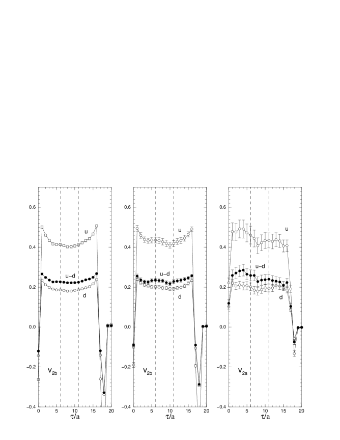
Figure 5: $v_{2b}$ versus $\tau/a$ from the ratios $R(17a,\tau;\vec{0};{\cal O}_{v_{2b}})$, $R(17a,\tau;\vec{p}_{1};{\cal O}_{v_{2b}})$, eq. (41) left and middle pictures respectively and $v_{2a}$ from $R(17a,\tau;\vec{p}_{1};{\cal O}_{v_{2a}})$, right picture for ${\cal O}^{(u)}$, ${\cal O}^{(d)}$ (empty circles) and NS (ie ${\cal O}^{(u)}-{\cal O}^{(d)}$) (filled circles) for $\beta=6.2$ at $\kappa=0.1344$. The chosen fit intervals are denoted by vertical dotted lines.

$R(17a,\tau;\vec{0};{\cal O}_{v_{2b}})$, $R(17a,\tau;\vec{p}_{1};{\cal O}_{v_{2b}})$, $R(17a,\tau;\vec{p}_{1};{\cal O}_{v_{2a}})$, left to right pictures respectively, for $\beta=6.2$ and $\kappa=0.1344$. We seek a plateau in the region $0\ll\tau/a\ll 17$. The region chosen is denoted by vertically dashed lines. Clearly the operator corresponding to $v_{2b}$ delivers a better signal for the ratio than the operator for $v_{2a}$, although even for the $v_{2b}$ operator we see that it is better to choose zero momentum rather than non-zero momentum.

In this section, as mentioned before, we wish to merely estimate the numerical significance of extra operators, as described in section 4.2. To this end, as mixing coefficients and improvement coefficients are not so well known, we make a series of plots either comparing the ratio of the additional improvement operators (ie the $v_{n}$ constructed using the ${\cal O}^{(i)}$ in eqs. (37) and (41)) to the original operator,

$$r^{i}_{v_{n}}\equiv{v_{n}^{i}\over v_{n}}\,,$$ (42)

or compare directly the $v_{n}^{m_{i}}$ derived from eqs. (34), (• ‣ 4.2.1) to the original operator, $v_{n}$. (It will be seen in section 5 that the ratios $r^{i}_{v_{n}}$ have a physical significance.)

These are all plotted against the square of the pseudoscalar meson mass. As $(am_{ps})^{2}$ is proportional to the quark mass for small quark mass, using this quantity avoided the necessity of first determining the critical hopping parameter $\kappa_{c}$ in the quark mass definition, eq. (38). We have thus used the (dimensionless) extrapolation parameter $(r_{0}/a)^{2}\times(am_{ps})^{2}\equiv(r_{0}m_{ps})^{2}$, with $r_{0}/a$ being given by the Padé formula in [38]. Using $r_{0}=0.5\,\mbox{fm}$ this enables us to get an idea of how close our simulation points are to the chiral limit in physical units.

4.4.1 $v_{2}$

In Fig. 6

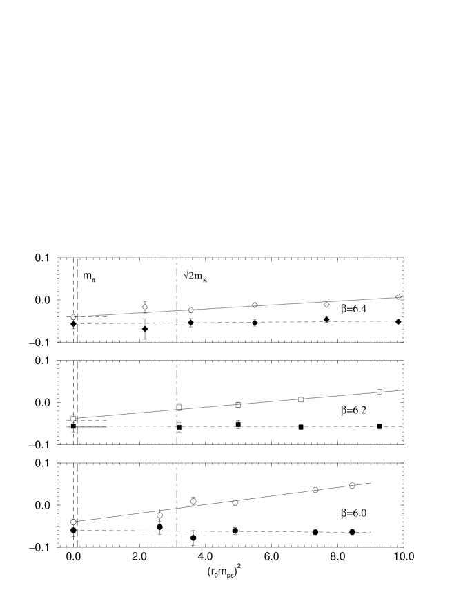
Figure 6: The ratios $ar^{1}_{v_{2a}}$, $ar^{2}_{v_{2a}}$ plotted against $(r_{0}m_{ps})^{2}$. The filled symbols at non-zero $(r_{0}m_{ps})^{2}$ are for $ar^{1}_{v_{2a}}$, while the empty symbols denote $ar^{2}_{v_{2a}}$. Also shown is a linear chiral extrapolation (dashed line and full line for $ar^{1}_{v_{2a}}$, $ar^{2}_{v_{2a}}$ respectively). The result in the chiral limit $(r_{0}m_{ps})^{2}\equiv 0$ is also indicated, again using full, empty symbols for $ar^{1}_{v_{2a}}$, $ar^{2}_{v_{2a}}$ respectively. The small horizontal lines around the chiral limit represent the perturbative estimate, see section 5, with again a dashed line corresponding to $ar^{1}_{v_{2a}}$ and a full line to $ar^{2}_{v_{2a}}$ respectively. The rough values of the (hypothetical) pseudoscalar mass composed from $u/d$ or $s$ quark masses, evaluated from $m_{\pi}$ and $m_{K}$ respectively are shown as dashed vertical lines.

we show $ar_{2a}^{1}$, $ar_{2a}^{2}$ plotted against $(r_{0}m_{ps})^{2}$, together with a linear chiral extrapolation. Also plotted is the approximate value of the pseudoscalar mass corresponding to degenerate $u/d$ or $s$ quark masses. So we see that our simulation runs over the range from about two to three times the strange quark mass to a little under the strange quark mass. It is also noticeable that we are a long way from simulating with a light $u/d$ quark mass – in fact within our errors, there is no difference between linearly extrapolating to the chiral limit or to the pion mass. Nevertheless we see that the effect of any extra improvement operators is likely to be small, of the order of a few percent.

The above result is for the off-diagonal operator, which needs a non-zero momentum in its evaluation. This figure is to be compared with the result using the diagonal operator, which advantageously may use zero momentum. In Fig. 7

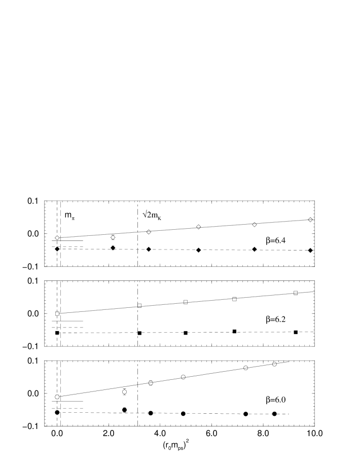
Figure 7: $ar^{1}_{v_{2b}}$, $ar^{2}_{v_{2b}}$ versus $(r_{0}m_{ps})^{2}$ for $\beta=6.0$, $6.2$ and $6.4$ with $\vec{p}=\vec{0}$. The notation is the same as for Fig. 6.

we show this result. In comparison with the previous picture, the errors are considerably reduced, as $\vec{p}=0$ is used (see also Fig. 5). Indeed using $\vec{p}=\vec{p}_{1}$ (see Appendix D for the numbers) we see that the errors grow again, although they are never as large as for the off-diagonal operator. Again, the effect of any extra improvement operators is small.

Thus all the numerical results and linearly chirally extrapolated results for $ar^{i}_{v_{2}}$ look small giving $av_{2}^{i}\mathrel{\hbox to0.0pt{\lower 4.0pt\hbox{\hskip 1.0pt$\sim$}\hss}\raise 1.0pt\hbox{$<$}}5\%$ of $v_{2}$ and some indeed are consistent with zero. From eq. (39), we see that if we choose $c_{2}=0$ then $c_{1}\equiv O(g_{0}^{2})$, which is likely to be small. So these results lead numerically to a small additional improvement term and we conclude that the effect of these terms in $v_{2}$ can be assumed to be negligible.

4.4.2 $v_{3}$ and $v_{4}$

We now present our results for the higher moments. In Fig. 8

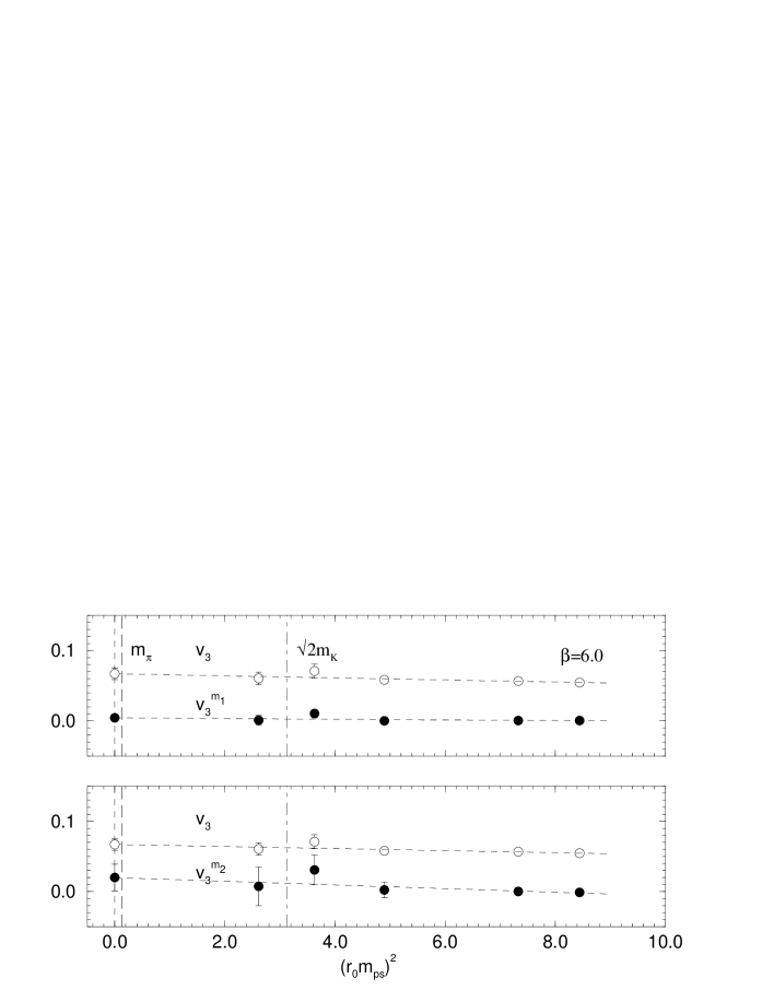
Figure 8: Mixing terms, $v_{3}^{m_{1}}$, $v_{3}^{m_{2}}$ for $\beta=6.0$ (filled circles). Also shown is $v_{3}$ (open circles) and linear chiral extrapolations. The same notation as for Fig. 6.

we show $v_{3}^{m_{1}}$, $v_{3}^{m_{2}}$ for $\beta=6.0$, together with a linear chiral extrapolation. Also shown, for comparison, is the operator $v_{3}$. As expected while the magnitude of the noise has increased in comparison with $v_{2}$ and scatters more, an acceptable signal is still seen. We find a clear separation between $v_{3}$ and the mixing operators (indeed they are consistent with $\approx 0$). For higher $\beta$ values, the data fluctuates more and it becomes more difficult to disentangle the results.

In Fig. 9 we plot $v_{4}^{m_{1}}$,

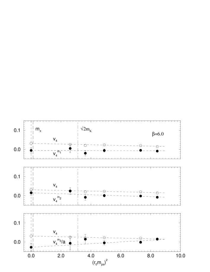
Figure 9: $v_{4}$ for $\beta=6.0$ together with $v_{4}^{m_{1}}$, $v_{4}^{m_{2}}$, $v_{4}^{m_{3}}/a$. The notation is the same as for Fig. 6.

$v_{4}^{m_{2}}$, $v_{4}^{m_{3}}/a$, together with $v_{4}$. While there is a reasonable signal for $v_{4}$, the improvement terms fluctuate a lot (again becoming worse the higher the value of $\beta$ is). Indeed even finding a plateau for the ratio $R(t,\tau;\vec{p};{\cal O})$ in eq. (40) becomes problematical. It would appear that while, numerically, $v_{4}^{m_{1}}$, $v_{4}^{m_{2}}$ are small in comparison with $v_{4}$ the situation is less clear cut for $v_{4}^{m_{3}}/a$ (although it is only including the heaviest quark mass point that leads to a non-zero result in the chiral limit). Nevertheless as most of the results for the mixing terms are much smaller than $v_{4}$ we shall ignore any effects from them.

5 Operator renormalisation

A lattice operator (or matrix element) must, in general, be renormalised. Again, we shall discuss mixing and $O(a)$ operator improvement separately.

5.1 Operator mixing and renormalisation

For operator mixing we can generally write

$${\cal O}^{\cal S}_{i}(M)=\sum_{j}Z_{{\cal O}_{i}{\cal O}_{j};\mbox{\tiny$L\!A\!T$}}^{\phantom{{\cal O}_{i}{\cal O}_{j};}\cal S}(M,a){\cal O}_{j}^{\mbox{\tiny$L\!A\!T$}}(a)\,,$$ (43)

working in a scheme ${\cal S}$ at scale $M$. So we must determine a matrix of renormalisation constants. While for those mixing operators of the same dimension as the original operator, low order perturbation results can be calculated (at least in principle), for lower dimensional operators this is not reliable: the renormalisation constant is proportional to a positive power of $1/a$ and non-perturbative terms may contribute. For the higher moments, both cases occur. For $v_{3}$ both the $m_{1}$ and $m_{2}$ operators have the same dimension as the original operator, and for $v_{4}$, $m_{1}$ and $m_{2}$ have the same dimension, while $m_{3}$ is dimension one lower, see eqs. (34), (• ‣ 4.2.1).

5.1.1 Renormalisation and relevant operator mixing

In this section we want to make a few comments on the operator mixings seen for the operators we use in this paper, and contrast them with the mixing problems for the operators which we rejected.

In the continuum, symmetry under $O(4)$ in the Euclidean case (or the Lorentz group in the Minkowski case) imposes strong constraints on which operators can have unpolarised forward nucleon matrix elements. One way of stating the rule is to say that the only operators with non-zero unpolarised forward matrix elements are those which have $J^{P}=0^{+}$ in the nucleon’s rest frame. The quantum numbers $J^{P}=0^{+}$ only occur in $O(4)$ representations of the form $U_{+}^{(\mu,\mu)}$ in the notation of [39]. Considering the $O(4)$ classification of the operators is relevant, because although bare lattice matrix elements only respect the symmetries of the hypercubic group $H(4)$, renormalised quantities should respect the full continuum symmetry group.

If we look at the mixing operators for $v_{3}$, as listed in eq. (34), we see that under the hypercubic group they transform exactly the same way as $v_{3}$, but under $O(4)$ they both transform according to the representation $U^{(\mbox{\small$\frac{1}{2}$},\mbox{\small$\frac{3}{2}$})}$, which means that by the continuum symmetries their renormalised forward matrix elements must be zero,

$$v_{3}^{m_{i};{\cal S}}=0\,.$$ (44)

Similarly the mixing operators for $v_{4}$, listed in eq. (• ‣ 4.2.1), all transform according to the $U^{(0,2)}$ representation of $O(4)$, so

$$v_{4}^{m_{i};{\cal S}}=0\,.$$ (45)

If the renormalised mixing operators all have the value zero, we can express all the bare lattice matrix elements in terms of a single renormalised matrix element. Again taking the $v_{3}$ system as our exemplar,

$$v_{3} = \left(Z^{-1}\right)_{v_{3};v_{3}}v_{3}^{\cal S}\,,$$

$$v_{3}^{m_{i}} = \left(Z^{-1}\right)_{v_{3}^{m_{i}};v_{3}}v_{3}^{\cal S}\,,$$ (46)

(temporarily dropping, for clarity, other arguments of the renormalisation constants). Since all the lattice matrix elements are multiples of the physically interesting matrix element $v_{3}^{\cal S}$ we have a choice in how we calculate the renormalised matrix element. We could add up all the terms in eq. (43), assuming that we know the mixing $Z$s well enough. Or we could equally well just invert eq. (46) and calculate $v_{3}^{\cal S}$ from $v_{3}$ alone,

$$v_{3}^{\cal S}={v_{3}\over\left(Z^{-1}\right)_{v_{3};v_{3}}}\,.$$ (47)

If we calculate the renormalised matrix element from $v_{3}$ alone, we should really renormalise by dividing by $(Z^{-1})_{v_{3};v_{3}}$ instead of multiplying by $Z_{v_{3};v_{3}}$. In practice the difference is minor,

$${1\over\left(Z^{-1}\right)_{v_{3};v_{3}}}\approx Z_{v_{3};v_{3}}-\sum_{i}{Z_{v_{3};v_{3}^{m_{i}}}Z_{v_{3}^{m_{i}};v_{3}}\over Z_{v_{3}^{m_{i}};v_{3}^{m_{i}}}}\,.$$ (48)

The difference involves the product of two off-diagonal $Z$s, and so is ${\cal O}(g_{0}^{4})$ in perturbation theory, see section 5.2.1, and is still likely to be tiny non-perturbatively. Note that eq. (48) tells us that mixing with lower dimension operators is no more dangerous than mixing with operators of the same dimension, in a case like this where the lower-dimensional operator has zero renormalised matrix element. This is because the product $Z_{v_{3};v_{3}^{m_{i}}}Z_{v_{3}^{m_{i}};v_{3}}$ is dimensionless, even when $v_{3}^{m_{i}}$ is a lower dimensional operator.

We conclude that for the operators we use in this paper, mixing is relatively benign, because continuum symmetry says that the renormalised mixing matrix elements are zero.

Finally we want to contrast this with an example where this is not so, to show the importance of choosing the operators carefully. We could have tried to measure $v_{3}$ with the operator

$$O^{\gamma}_{\{444\}}-O^{\gamma}_{\{411\}}-O^{\gamma}_{\{422\}}-O^{\gamma}_{\{433\}}\;.$$ (49)

This however would have much worse mixing problems because it mixes with operators which are allowed to have nucleon matrix elements in the continuum, for example

$$O^{\gamma}_{\{444\}}+O^{\gamma}_{\{411\}}+O^{\gamma}_{\{422\}}+O^{\gamma}_{\{433\}}\,,\quad\overline{q}\gamma_{4}q\quad\hbox{ or }\quad\overline{q}\stackrel{{\scriptstyle\leftrightarrow}}{{D}}_{4}q\;.$$ (50)

Now we would not have the option of using eq. (47), we would have to use eq. (43) and to get a reliable answer we would need to know the off-diagonal elements of $Z$ accurately (especially those for the operators of lower dimension). This is why we rejected the operator eq. (49), and why we think that the mixing operators of subsection 4.2.1 are not a problem.

5.1.2 Renormalisation and operator improvement

For $O(a)$ improved operators, we know that the operator depends linearly on the improvement coefficients $c_{i}$ as shown in eq. (37). Our experience from extensive perturbative calculations in [34] leads us to expect a result of the form

$$\Lambda_{{\cal O}^{i}}^{\mbox{\tiny$L\!A\!T$}}={\zeta_{i}\over a}\Lambda_{\cal O}^{\mbox{\tiny$L\!A\!T$}}+O(a^{0})\,,$$ (51)

where $\Lambda^{\mbox{\tiny$L\!A\!T$}}$ is the lattice amputated three-point Green’s function, ${\cal O}$ is the relevant operator and ${\cal O}^{i}$ are the improvement or irrelevant operators in eq. (37). (Note that there is nothing forbidding the improvement terms mixing with ${\cal O}/a$.) The only case that does not mix is the mass improvement term $am_{q}{\cal O}$,

$$am_{q}\Lambda_{\cal O}^{\mbox{\tiny$L\!A\!T$}}=O(a)\,.$$ (52)

We can calculate the $c_{i}$ dependence of the renormalisation constant by requiring that the renormalised $\Lambda^{\cal S}_{\cal O}$ should be independent of the $c_{i}$ at leading order in $a$ and thus we have (temporarily suppressing additional $M$, $a$ arguments)

$$\Lambda^{\cal S}_{\cal O} = {Z_{\cal O;\mbox{\tiny$L\!A\!T$}}^{\phantom{{\cal O};}\cal S}(\{c_{i}\})\over Z_{q;\mbox{\tiny$L\!A\!T$}}^{\phantom{q;}{\cal S}}}\Big{[}\Lambda^{\mbox{\tiny$L\!A\!T$}}_{\cal O}+\sum_{i\not=0}c_{i}\zeta_{i}\Lambda^{\mbox{\tiny$L\!A\!T$}}_{\cal O}+O(a)\Big{]}\,,$$ (53)

$$= {Z_{\cal O;\mbox{\tiny$L\!A\!T$}}^{\phantom{{\cal O};}\cal S}(\{c_{i}\})\over Z_{q;\mbox{\tiny$L\!A\!T$}}^{\phantom{q;}{\cal S}}}\Big{(}1+\sum_{i\not=0}c_{i}\zeta_{i}\Big{)}\Lambda^{\mbox{\tiny$L\!A\!T$}}_{\cal O}+O(a)\,,$$

$$\equiv {Z_{\cal O;\mbox{\tiny$L\!A\!T$}}^{\phantom{{\cal O};}\cal S}(\{0\})\over Z_{q;\mbox{\tiny$L\!A\!T$}}^{\phantom{q;}{\cal S}}}\Lambda^{\mbox{\tiny$L\!A\!T$}}_{\cal O}+O(a)\,,$$

and so we can write

$${\cal O}^{\cal S}(M)=Z_{\cal O;\mbox{\tiny$L\!A\!T$}}^{\phantom{{\cal O};}\cal S}(M,a,\{c_{i}\}){\cal O}(a,\{c_{i}\},c_{0})\equiv{Z_{\cal O;\mbox{\tiny$L\!A\!T$}}^{\phantom{{\cal O};}\cal S}(M,a,\{0\})\over 1+\sum_{i\neq 0}c_{i}\zeta_{i}}{\cal O}(a;\{c_{i}\},c_{0})\,,$$ (54)

where the coefficients $\zeta_{i}\equiv\zeta_{i}(g_{0})=O(g_{0}^{2})$ have to be determined. Again in [34] we have given these coefficients for $v_{2a}$ and $v_{2b}$ in lowest order perturbation theory using eq. (51). (Requiring $O(a)$ improvement also determines the $c_{i}$ as given for example in eq. (39).) Numerically these coefficients turn out to be quite small. In addition to the perturbative $\zeta_{i}$’s we can also find non-perturbative $\zeta_{i}$’s by looking at our measured nucleon matrix elements and requiring that the improved result and the unimproved agree to leading order in $a$, ie from eq. (54) we have

$${v_{n}+a\sum_{i\neq 0}c_{i}v_{n}^{i}\over 1+\sum_{i\neq 0}c_{i}\zeta_{i}}=v_{n}+O(a)\,,$$ (55)

giving, cf eq. (51),

$$v_{n}^{i}={1\over a}\zeta_{i}v_{n}+O(a^{0})\,,$$ (56)

or

$$\zeta_{i}=\left.ar^{i}_{v_{n}}\right|_{am_{q}=0}+O(a)\,,$$ (57)

(see eq. (42)). We would expect $\zeta_{i}$ calculated in this way to agree up to ambiguities of $O(a)$. In Fig. 6 and Fig. 7 we compare the values for $\zeta_{i}$ obtained this way with the $1$-loop perturbative results from [34] (shown in the figures as short horizontal lines about the chiral limit). Although, not unexpectedly, there are differences to the perturbative result, the ratios remain small. From eq. (39) we may choose $c_{2}=0$ and so $c_{1}=O(g_{0}^{2})$ is also small. Hence the change in the denominator of eq. (54) from $1$ is small and so does not change the renormalisation constant perceptibly. Thus we shall ignore any small effects here (just as in section 4.4, where our conclusion was that we could numerically drop the $O(a)$ improvement terms).

5.2 Determining the renormalisation constants

To define the renormalisation constants a renormalisation procedure must be prescribed. Often the renormalisation constants are defined first in a MOM scheme by computing the (Landau) gauge fixed two-quark Green’s function with one operator insertion and setting

$$\left[\Lambda^{\mbox{\tiny$M\!O\!M$}}_{{\cal O}}\right]_{p^{2}=\mu_{p}^{2}}=\left.\Lambda^{\mbox{\tiny$M\!O\!M$}}_{{\cal O}}\right|_{\mbox{\tiny$B\!O\!R\!N$}}\,,$$ (58)

where $\Lambda^{\mbox{\tiny$M\!O\!M$}}_{{\cal O}}$ is the (renormalised) amputated three-point Green’s function for the operator $\cal O$. The RHS of this equation is the tree level value (or Born approximation) of the amputated function. This definition may be used for perturbative computations, see eg [40], where $[\ldots]$ in eq. (58) means that, in a given basis, we drop terms not proportional to the Born term. This may be modified, using a trace condition for the definition of the renormalisation constants, to give the alternative $\rm{RI}^{\prime}-\rm{MOM}$ scheme [41] which is also suitable for non-perturbative calculations. A discussion and some results for this non-perturbative method will be given in section 5.2.3.

The resulting $Z_{{\cal O}_{i};\mbox{\tiny$L\!A\!T$}}^{\phantom{{\cal O};}\mbox{\tiny$M\!O\!M$}}$ may, if wished, be converted to another scheme, ie to the $\overline{MS}$ scheme using eq. (12) where $Z_{{\cal O}_{i};{\cal O}_{j};\mbox{\tiny$M\!O\!M$}}^{\phantom{{\cal O}_{i}{\cal O}_{j};}\mbox{\tiny$\overline{MS}$}}(\mu,\mu_{p})$ is (perturbatively) calculable. The ${\overline{MS}}$ scheme is particularly convenient, as the renormalisation constants are independent of the gauge fixing condition chosen.

Unfortunately, the definition given in eq. (58) has its limitations: ${\cal O}^{m_{2}}_{v_{3}}$, ${\cal O}^{m_{1}}_{v_{4}}$ ${\cal O}^{m_{2}}_{v_{4}}$ and ${\cal O}^{m_{3}}_{v_{4}}$ all have vanishing Born matrix elements between quark states (as they involve commutators of covariant derivatives). So in order to be able to compute the renormalisation constants we would have to consider more general Green’s functions (eg quark-gluon). At present we must simply ignore this problem though.

After these more general remarks, we shall now give various results for the renormalisation constants for (one-loop) perturbation theory, TRB perturbation theory and finally a non-perturbative determination of the relevant constants.

5.2.1 Perturbation Theory

One loop perturbation theory yields

$$Z_{{\cal O}_{i};{\cal O}_{j};\mbox{\tiny$L\!A\!T$}}^{\phantom{{\cal O}_{i};{\cal O}_{j};}\cal S}(M,a)=\delta_{{\cal O}_{i};{\cal O}_{j}}+g_{0}^{2}\left[d_{{\cal O}_{i};{\cal O}_{j};0}\ln(aM)-B^{\cal S}_{{\cal O}_{i};{\cal O}_{j}}(c_{sw})\right]+O(g_{0}^{4})\,.$$ (59)

In the $\overline{MS}$ scheme ($M\equiv\mu$) we have, [34],

$$B^{\mbox{\tiny$\overline{MS}$}}_{v_{2a}}(c_{sw}) = {C_{F}\over(4\pi)^{2}}\left(1.27959-3.87297c_{sw}-0.67826c_{sw}^{2}\right)\,,$$

$$B^{\mbox{\tiny$\overline{MS}$}}_{v_{2b}}(c_{sw}) = {C_{F}\over(4\pi)^{2}}\left(2.56184-3.96980c_{sw}-1.03973c_{sw}^{2}\right)\,,$$ (60)

with $C_{F}=4/3$. The calculations have been extended by S. Capitani [43] to now include $B^{\mbox{\tiny$\overline{MS}$}}_{v_{3}}$, $B^{\mbox{\tiny$\overline{MS}$}}_{v_{4}}$. For ${\cal O}_{v_{3}}$, off-diagonal elements in eq. (59) have also been computed

$$B^{\mbox{\tiny$\overline{MS}$}}_{v_{3}}(c_{sw}) = {C_{F}\over(4\pi)^{2}}\left(-12.12740-2.92169c_{sw}-0.98166c_{sw}^{2}\right)\,,$$

$$B^{\mbox{\tiny$\overline{MS}$}}_{v_{3};v_{3}^{m_{1}}}(c_{sw}) = {C_{F}\over(4\pi)^{2}}\left(-0.36848-0.032760c_{sw}+0.029137c_{sw}^{2}\right)\,,$$

$$B^{\mbox{\tiny$\overline{MS}$}}_{v_{3}^{m_{1}}}(c_{sw}) = {C_{F}\over(4\pi)^{2}}\left(-14.85157-2.15228c_{sw}-1.70741c_{sw}^{2}\right)\,,$$

$$B^{\mbox{\tiny$\overline{MS}$}}_{v_{3}^{m_{1}};v_{3}}(c_{sw}) = {C_{F}\over(4\pi)^{2}}\left(-3.30605+0.33335c_{sw}-0.37050c_{sw}^{2}\right)\,.$$ (61)

For $B^{\mbox{\tiny$\overline{MS}$}}_{v_{4}}$ we have

$$B^{\mbox{\tiny$\overline{MS}$}}_{v_{4}}(c_{sw})={C_{F}\over(4\pi)^{2}}\left(-25.50303-2.41788c_{sw}-1.12826c_{sw}^{2}\right)\,.$$ (62)

The lowest order anomalous dimension coefficient, being universal, is given for the three moments by eq. (21) and in our basis the coefficients $d_{v_{3};v_{3}^{m_{1}};0}$ and $d_{v_{3}^{m_{1}};v_{3};0}=0$ vanish, while $d_{v_{3}^{m_{1}};0}=-28/(9(4\pi)^{2})$.

For consistency at this order in perturbation theory, we take $c_{sw}=1$ (the tree level value). Setting $\mu=1/a$ to avoid large logarithmic factors gives, for example at $\beta=6.0$, the results

$$Z_{v_{2a};\mbox{\tiny$L\!A\!T$}}^{\phantom{v_{2a};}\mbox{\tiny$\overline{MS}$}} = 1.0276\,,$$

$$Z_{v_{2b};\mbox{\tiny$L\!A\!T$}}^{\phantom{v_{2b};}\mbox{\tiny$\overline{MS}$}} = 1.0207\,,$$

$$Z_{v_{3};\mbox{\tiny$L\!A\!T$}}^{\phantom{v_{3};}\mbox{\tiny$\overline{MS}$}} = 1.1354,\qquad Z_{v_{3};v_{3}^{m_{1}};\mbox{\tiny$L\!A\!T$}}^{\phantom{v_{3};v_{3}^{m_{1}};}\mbox{\tiny$\overline{MS}$}}=0.003142\,,$$

$$Z_{v_{4};\mbox{\tiny$L\!A\!T$}}^{\phantom{v_{4};}\mbox{\tiny$\overline{MS}$}} = 1.2453\,.$$ (63)

While we see that for $v_{2}$ first order perturbation theory changes the tree level result ($\equiv 1$) very little, there are perceptible differences for the higher moments. Note also that the mixing renormalisation constant for $v_{3}$ is very small in comparison to the diagonal renormalisation constant, $Z_{v_{3};\mbox{\tiny$L\!A\!T$}}^{\phantom{v_{3};}\mbox{\tiny$\overline{MS}$}}$. In addition, although the mixing operator signal is rather noisy, $v_{3}^{m_{1}}\ll v_{3}$ as we have seen in section 4.4.2. Thus assuming that for a non-perturbative evaluation $Z_{v_{3};\mbox{\tiny$L\!A\!T$}}^{\phantom{v_{3};}\mbox{\tiny$\overline{MS}$}}\gg Z_{v_{3};v_{3}^{m_{1}};\mbox{\tiny$L\!A\!T$}}^{\phantom{v_{3};v_{3}^{m_{1}};}\mbox{\tiny$\overline{MS}$}}$ (as is the case for the perturbative result), we can ignore the effects of the mixing term in the future.

We also use the three loop result from Table 6 for $\Delta Z_{v_{n}}^{\mbox{\tiny$\overline{MS}$}}(\mu)$ to find the RGI factor $Z^{\mbox{\tiny$R\!G\!I$}}_{v_{n}}$, eq. (15).

5.2.2 TRB perturbation theory

To improve the perturbative renormalisation results of the last section, we shall apply tadpole-improved renormalisation-group-improved boosted perturbation theory or TRB-PT, [45], which we shall now describe. The renormalised operator is given by

$${\cal O}^{\mbox{\tiny$\overline{MS}$}}(\mu)=Z^{\phantom{{\cal O};}\mbox{\tiny$\overline{MS}$}}_{{\cal O};\mbox{\tiny$L\!A\!T$}}(\mu,a){\cal O}(a)\,.$$ (64)

As in eq. (11), we may define a $\gamma$ function either in the $\overline{MS}$ scheme or what we shall formally call here the $LAT$ scheme. Additionally as expansions in the bare coupling constant seem to be badly convergent, we choose to expand in the boosted coupling constant and thus we have

$$\left.{\partial\over\partial\log a}\log Z^{\phantom{{\cal O};}\mbox{\tiny$\overline{MS}$}}_{{\cal O};\mbox{\tiny$L\!A\!T$}}(\mu,a)\right|_{\mu}=\gamma^{\mbox{\tiny$L\!A\!T$}}_{\cal O}(g_{\Box})=d_{{\cal O};0}g_{\Box}^{2}+d^{\mbox{\tiny$L\!A\!T$}}_{{\cal O};1}g_{\Box}^{4}+\ldots\,,$$ (65)

where

$$g^{2}_{\Box}={g_{0}^{2}\over u_{0}^{4}}\,,\qquad u_{0}^{4}=\langle\mbox{\small$\frac{1}{3}$}\mbox{Tr}U^{\Box}\rangle\,,$$ (66)

and $U^{\Box}$ is the product of links around an elementary plaquette. Expanding $u_{0}$ we have $u_{0}=1-\mbox{\small$\frac{1}{4}$}g_{0}^{2}p_{1}+O(g_{0}^{4})$ where $p_{1}=1/3$.

From eq. (13), ie integrating eq. (11) for $({\cal S},M)\equiv(\overline{MS},\mu)$ and $(LAT,a^{-1})$, eq. (65), gives

$$Z^{\phantom{{\cal O};}\mbox{\tiny$\overline{MS}$}}_{{\cal O};\mbox{\tiny$L\!A\!T$}}(\mu,a)={\Delta Z^{\mbox{\tiny$L\!A\!T$}}_{\cal O}(a)\over\Delta Z^{\mbox{\tiny$\overline{MS}$}}_{\cal O}(\mu)}\,,$$ (67)

and thus from eq. (64), the RGI quantity may be written as

$${\cal O}^{\mbox{\tiny$R\!G\!I$}}=\Delta Z^{\mbox{\tiny$\overline{MS}$}}_{\cal O}(\mu){\cal O}^{\mbox{\tiny$\overline{MS}$}}(\mu)=\Delta Z^{\mbox{\tiny$L\!A\!T$}}_{\cal O}(a){\cal O}(a)\,.$$ (68)

Expanding eq. (67) and comparing with eq. (59) enables an expression to be found for $d_{{\cal O};1}^{\mbox{\tiny$L\!A\!T$}}$ of

$$d_{{\cal O};1}^{\mbox{\tiny$L\!A\!T$}}=d_{{\cal O};1}^{\mbox{\tiny$\overline{MS}$}}+d_{{\cal O};0}(t_{1}-p_{1})-2b_{0}B^{\mbox{\tiny$\overline{MS}$}}_{\cal O}(1)\,,$$ (69)

for $O(a)$ improved Wilson fermions and where

$$g^{\mbox{\tiny$\overline{MS}$}}=g_{0}\left(1+\mbox{\small$\frac{1}{2}$}t_{1}g_{0}^{2}+\ldots\right)\,,$$ (70)

at the scale $\mu=1/a$. $t_{1}$ is known and is given by $t_{1}=0.468201$, [46]. Hence $d_{{\cal O};1}^{\mbox{\tiny$L\!A\!T$}}$ may be computed. Values are given in Table 3.

${\cal O}$	$d_{{\cal O};1}^{\mbox{\tiny$L\!A\!T$}}$
$v_{2a}$	$-152.14/(4\pi)^{4}$
$v_{2b}$	$-176.31/(4\pi)^{4}$
$v_{3}$	$91.828/(4\pi)^{4}$
$v_{4}$	$382.32/(4\pi)^{4}$

Table 3: Values of $d_{{\cal O};1}^{\mbox{\tiny$L\!A\!T$}}$ for $O(a)$ improved fermions from eq. (69).

For two loops a simple exact analytic expression is possible for $\Delta Z^{\cal S}_{\cal O}(M)$ of

$$\Delta Z^{\mbox{\tiny$L\!A\!T$}}_{\cal O}(a)=\left[2b_{0}g^{2}_{\Box}\right]^{d_{{\cal O};0}\over 2b_{0}}\left[1+{b_{1}\over b_{0}}g^{2}_{\Box}\right]^{b_{0}d_{{\cal O};1}^{\mbox{\tiny$L\!A\!T$}}-b_{1}d_{{\cal O};0}\over 2b_{0}b_{1}}\,.$$ (71)

The expression in eq. (71) is the result of renormalisation-group-improved boosted perturbation theory. We can finally tadpole improve it to obtain to this order

$$\Delta Z^{\mbox{\tiny$L\!A\!T$}}_{\cal O}(a)=u_{0}^{1-n_{D}}\left[2b_{0}g^{2}_{\Box}\right]^{d_{{\cal O};0}\over 2b_{0}}\left[1+{b_{1}\over b_{0}}g^{2}_{\Box}\right]^{{b_{0}d_{{\cal O};1}^{\mbox{\tiny$L\!A\!T$}}-b_{1}d_{{\cal O};0}\over 2b_{0}b_{1}}+{p_{1}\over 4}{b_{0}\over b_{1}}\left(1-n_{D}\right)}\,,$$ (72)

where $n_{D}$ is the number of derivatives in the operator. Note that for one derivative operators, TI has no effect, ie eq. (71) is the same as eq. (72). Again we have the factor, eq. (15),

$$Z^{\mbox{\tiny$R\!G\!I$}}_{\cal O}(a)\equiv\Delta Z^{\mbox{\tiny$L\!A\!T$}}_{\cal O}(a).$$ (73)

Thus $\Delta Z^{\mbox{\tiny$L\!A\!T$}}_{\cal O}(a)$ is the function that takes you directly from the lattice result to the RGI result.

Finally if we additionally wish to TI the improvement coefficients, [34], then we replace $g_{0}^{2}$ by $g_{\Box}^{2}$ in eq. (39). Numerical results from this procedure for $c_{0}$ in $v_{2}$ with $c_{2}=0$ are given in Table 4. The associated $\kappa_{c}$, necessary for the computation of $am_{q}$, eq. (38) are given in [47].

5.2.3 Non-perturbative $Z$ determinations

We now look at the $\rm{RI}^{\prime}-\rm{MOM}$ non-perturbative determination of renormalisation constants, using the method proposed by Martinelli et al [41] which mimics (up to a point) the approach of the perturbative lattice procedure, by defining

$$Z_{\cal O;\mbox{\tiny$L\!A\!T$}}^{\phantom{{\cal O};}\mbox{\tiny$R\!I^{\prime}\!\!-\!\!M\!O\!M$}}(\mu_{p},a)=\left.{Z_{q;\mbox{\tiny$L\!A\!T$}}^{\phantom{q;}\mbox{\tiny$R\!I^{\prime}\!\!-\!\!M\!O\!M$}}(p)\over\mbox{\small$\frac{1}{12}$}\mbox{Tr}\left[\Lambda_{\cal O}(p)\Lambda_{{\cal O},\mbox{\tiny$B\!O\!R\!N$}}^{-1}(p)\right]}\right|_{p^{2}=\mu_{p}^{2}}\,,$$ (74)

where the wave function renormalisation constant $Z_{q;\mbox{\tiny$L\!A\!T$}}^{\phantom{q;}\mbox{\tiny$R\!I^{\prime}\!\!-\!\!M\!O\!M$}}(p)$ can be fixed from the conserved vector current or from the (Fourier transformed) quark propagator $S_{q}(p)$ by

$$Z_{q;\mbox{\tiny$L\!A\!T$}}^{\phantom{q;}\mbox{\tiny$R\!I^{\prime}\!\!-\!\!M\!O\!M$}}(p)={\mbox{\rm Tr}(-i\sum_{\lambda}\gamma_{\lambda}\sin(ap_{\lambda})aS_{q}^{-1}(p))\over 12\sum_{\lambda}\sin^{2}(ap_{\lambda})}\,.$$ (75)

(There are still various possibilities for $Z_{q;\mbox{\tiny$L\!A\!T$}}$, see eg [48] for different definitions. Again $\Lambda_{\cal O}$ is the amputated three-point Green’s function for the operator ${\cal O}$.) For our implementation using a ‘momentum source’ see [49]. For the higher derivative operators considered here, this is a non-covariant renormalisation condition, depending on the momentum direction, [49, 50] (numerically this is a small effect for the momenta considered here).

The non-perturbative results for $Z_{\cal O;\mbox{\tiny$L\!A\!T$}}^{\phantom{{\cal O};}\mbox{\tiny$R\!I^{\prime}\!\!-\!\!M\!O\!M$}}$ should now be brought to an RGI form, which can only be done perturbatively. In order to avoid problems caused by the non-covariance of the renormalisation condition eq. (74) we first transform $Z_{\cal O;\mbox{\tiny$L\!A\!T$}}^{\phantom{{\cal O};}\mbox{\tiny$R\!I^{\prime}\!\!-\!\!M\!O\!M$}}$ (perturbatively) to a covariant scheme $\cal S$ like $\overline{MS}$ or $MOM$ employing a conversion factor of the form

$$1+c^{\cal S}_{1}(g^{\mbox{\tiny$\overline{MS}$}})^{2}+c^{\cal S}_{2}\left(g^{\mbox{\tiny$\overline{MS}$}}\right)^{4}+\ldots\,.$$ (76)

For ${\cal S}=\overline{MS}$ the general expression to one-loop order can be found in [49], while an explicit formula for $v_{2b}$ is given in [50].The one-loop expressions for ${\cal S}=MOM$ are also known. In the case of $v_{2a}$ and $v_{2b}$, three-loop expressions can be derived from [51] and will be used in the following.

In a second step, multiplying the resulting numbers by $\Delta Z_{\cal O}^{\cal S}$, we obtain $Z_{\cal O}^{\mbox{\tiny$R\!G\!I$}}$ (see eq. (15)). Thus $\Delta Z_{\cal O}^{\cal S}$ has to be found, which as in section 5.2.2 is again the computation of the perturbative coefficients of the anomalous dimension $\gamma^{\cal S}$. For ${\cal S}=\overline{MS}$ the anomalous dimension is known to three loops for $v_{2}$, $v_{3}$ and $v_{4}$. For ${\cal S}=MOM$ only the first two loops (or coefficients) are available in the case of $v_{3}$ and $v_{4}$, while in the case of $v_{2}$ we can make use of the three-loop calculation in [51]. For example, expanding in $g^{\mbox{\tiny$\overline{MS}$}}$, $\gamma_{\cal O}^{\cal S}=d_{{\cal O};0}(g^{\mbox{\tiny$\overline{MS}$}})^{2}+d_{{\cal O};1}^{\cal S}(g^{\mbox{\tiny$\overline{MS}$}})^{4}+\ldots$, we have to two loops, similarly to eq. (72),

$$\Delta Z_{\cal O}^{\cal S}=\left[2b_{0}(g^{\mbox{\tiny$\overline{MS}$}})^{2}\right]^{d_{{\cal O};0}\over 2b_{0}}\left[1+{b_{1}\over b_{0}}(g^{\mbox{\tiny$\overline{MS}$}})^{2}\right]^{b_{0}d_{{\cal O};1}^{\cal S}-b_{1}d_{{\cal O};0}\over 2b_{0}b_{1}}\,.$$ (77)

Depending on the choice of $\cal S$ and the coupling in which $\gamma^{\cal S}$ is expanded, there are several possibilities (of course equivalent if one knew the whole power series). We shall briefly describe two methods here (I and II), whose difference we shall use to estimate the potential error due to (unknown) higher terms in the perturbative expansion. In method I we choose ${\cal S}=\overline{MS}$ and expand in $g^{\mbox{\tiny$\overline{MS}$}}$. In method II we work in the $MOM$ scheme (see [49]), and therefore it may be more natural to expand in other coupling constants defined using momentum renormalisation conditions. In [52] several possibilities are given. We shall use here the coupling defined by using the three gluon vertex, the $\widetilde{MOM}gg$ scheme, in the notation of [52].

If we plot $Z^{\mbox{\tiny$R\!G\!I$}}_{v_{n}}$ against $(r_{0}\mu_{p})^{2}$ and the perturbative expressions are sufficently well known, we would expect to see a plateau where $Z^{\mbox{\tiny$R\!G\!I$}}_{v_{n}}$ is independent of $(r_{0}\mu_{p})^{2}$. This region occurs when $\mu_{p}$ is not too small $\sim\Lambda$ otherwise non-perturbative effects play a role, nor when it is too large as lattice artifacts then occur. Unfortunately these $O(r_{0}\mu_{p})^{2}$ effects may become large (but depend very much on the operator considered). In perturbation theory in the chiral limit $O(a)$ terms of the Green’s function have opposite chirality to the leading term, they disappear when the trace in eq. (74) is taken. (For explicit lowest order results see [34].) Condensates may spoil this at low $\mu_{p}^{2}$, but here we are looking at higher momentum scales. Thus we shall take the plateaus in the chiral limit as our renormalisation constants.

We have made determinations of $Z_{{\cal O};\mbox{\tiny$L\!A\!T$}}^{\phantom{{\cal O};}\mbox{\tiny$R\!I^{\prime}\!\!-\!\!M\!O\!M$}}$ using eq. (74) for $\beta=6.0$, $6.2$ and $6.4$ on $24^{3}\times 48$, $24^{3}\times 48$, $32^{3}\times 40$ lattices respectively. For each $\beta$ three or more quark masses were used and a linear extrapolation in $am_{q}$ was performed to the chiral limit. More details will be given in [53].

5.3 Comparison of $Z^{\mbox{\tiny$R\!G\!I$}}$ results

We shall now use these results to find $Z^{\mbox{\tiny$R\!G\!I$}}_{v_{2}}$, $Z^{\mbox{\tiny$R\!G\!I$}}_{v_{3}}$ and $Z^{\mbox{\tiny$R\!G\!I$}}_{v_{4}}$. In Figs. 10, 11, 12 we plot $Z^{\mbox{\tiny$R\!G\!I$}}_{v_{2}}$, $Z^{\mbox{\tiny$R\!G\!I$}}_{v_{3}}$ and $Z^{\mbox{\tiny$R\!G\!I$}}_{v_{4}}$ for $\beta=6.2$ as computed from these techniques.

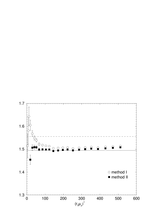
Figure 10: $Z^{\mbox{\tiny$R\!G\!I$}}_{v_{2b}}$ at $\beta=6.2$ versus $(r_{0}\mu_{p})^{2}$. NP method I is denoted by circles, while method II is given by filled squares. The dashed line is the TRB-PT result, while the full line is the NP estimate from method II.

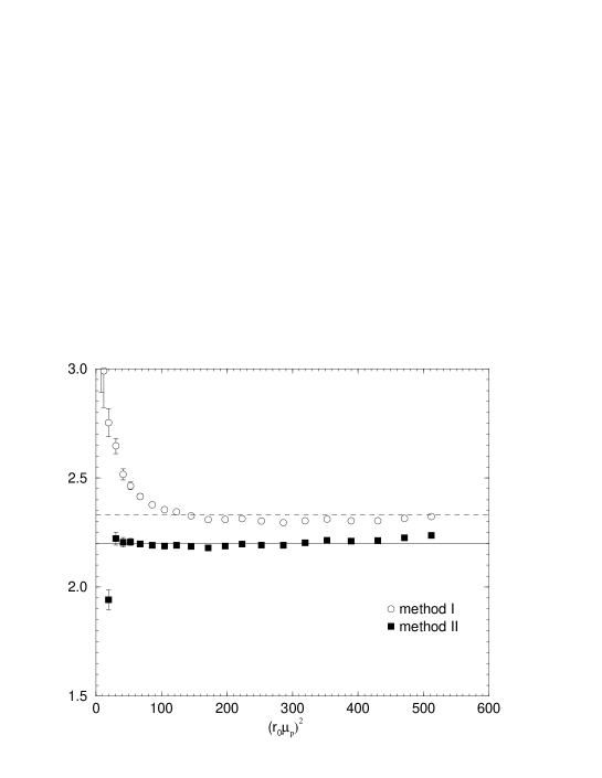
Figure 11: $Z^{\mbox{\tiny$R\!G\!I$}}_{v_{3}}$ at $\beta=6.2$ versus $(r_{0}\mu_{p})^{2}$. The same notation as for Fig. 10.

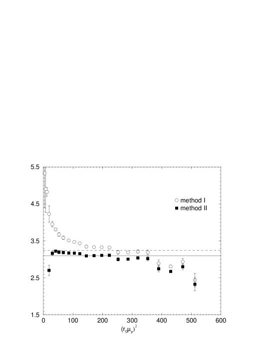
Figure 12: $Z^{\mbox{\tiny$R\!G\!I$}}_{v_{4}}$ at $\beta=6.2$ versus $(r_{0}\mu_{p})^{2}$. The same notation as for Fig. 10.

In the case of the non-perturbative $Z$s a reasonable plateau is seen for large $(r_{0}\mu_{p})^{2}$ enabling a value for the renormalisation constant to be found. Method II seems to reach a plateau faster than method I, so we shall use these results (taken around $\mu_{p}=5\,\mbox{GeV}$), with the difference to method I giving a rough estimate of the error. Also shown in the plots are the TRB-PT results. The NP and TRB-PT results lie close to each other, with a maximum discrepancy of about $8\%$. In the NP determination of the $Z$s, the plateaus become better as $\beta$ increases. This is shown in Fig. 13.

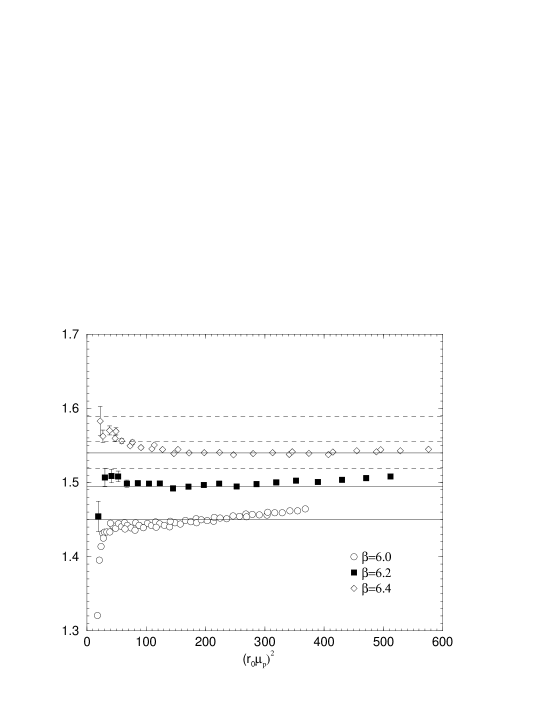
Figure 13: $Z^{\mbox{\tiny$R\!G\!I$}}_{v_{2b}}$ versus $(r_{0}\mu_{p})^{2}$ for $\beta=6.0$ (circles), $6.2$ (filled squares), $6.4$ (diamonds) using method II. The corresponding dashed lines are the TRB-PT results, while the full lines are the NP estimates.

In Table 4 we give the results from PT,

$\beta$		$6.0$	$6.2$	$6.4$
	PT	1.416	1.475	1.522
$Z^{\mbox{\tiny$R\!G\!I$}}_{v_{2a}}$	TRB-PT	1.536	1.571	1.604
	NP – I	1.46	1.51	1.56
	NP – II	1.45	1.50	1.55
$c^{\mbox{\tiny$T\!I$}}_{v_{2a};0}$	TI	1.232	1.218	1.205
	PT	1.407	1.465	1.513
$Z^{\mbox{\tiny$R\!G\!I$}}_{v_{2b}}$	TRB-PT	1.519	1.555	1.589
	NP – I	1.46	1.50	1.55
	NP – II	1.45	1.49	1.54
$c^{\mbox{\tiny$T\!I$}}_{v_{2b};0}$	TI	1.245	1.229	1.216
	PT	1.928	2.038	2.129
$Z^{\mbox{\tiny$R\!G\!I$}}_{v_{3}}$	TRB-PT	2.268	2.330	2.389
	NP – I	2.2	2.3	2.4
	NP – II	2.1	2.2	2.3
	PT	2.367	2.548	2.700
$Z^{\mbox{\tiny$R\!G\!I$}}_{v_{4}}$	TRB-PT	3.156	3.242	3.325
	NP – I	3.1	3.3	3.5
	NP – II	2.9	3.1	3.2

Table 4: $Z^{\mbox{\tiny$R\!G\!I$}}$ results (and some $c_{0}$ results) at $\beta=6.0$, $6.2$ and $6.4$, for $v_{n}$, $n=2$, $3$ and $4$. PT denotes the perturbative results from section 5.2.1 and TRB-PT from section 5.2.2. Note that to obtain $Z^{\mbox{\tiny$R\!G\!I$}}$ for PT the three-loop results from Table 6 have been used. Results from both NP variations, I and II are shown.

TRB-PT and NP method (both variants) for various renormalisation constants at $\beta=6.0$, $6.2$ and $6.4$.

6 Results: chiral and continuum extrapolations

6.1 The phenomenological approach

From the bare results given in Appendix D and the Zs in Table 4 we can now construct our renormalised matrix elements. As well as the continuum extrapolation $a\to 0$, as the quark masses presently used are rather heavy we also need to extrapolate these renormalised results to the chiral limit. In this section we shall consider both these limits. In Fig. 14

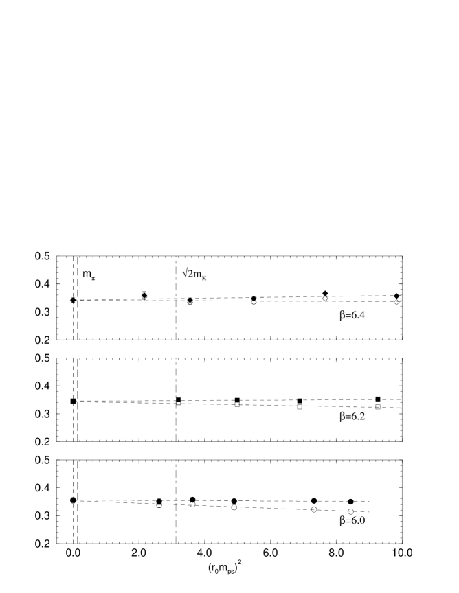
Figure 14: $v^{\mbox{\tiny$R\!G\!I$}}_{2b}$ versus $(r_{0}m_{ps})^{2}$ for $\beta=6.0$ (circles), $6.2$ (squares) and $6.4$ (diamonds). The filled symbols are obtained when using the TI value for $c_{0}$ while the empty symbols have $c_{0}=0$. Also shown are linear extrapolations to the chiral limit (dashed lines). Other notation as in Fig. 6.

we show the results for $v_{2b}$ for $\beta=6.0$, $6.2$ and $6.4$ with both $c_{0}=c_{0}^{\mbox{\tiny$T\!I$}}$, as given in Table 4, and $c_{0}=0$. (We would expect that for $c_{0}$ set to the TI value the results are practically $O(a)$ improved for non-zero quark mass.)

Also shown in the figure is a linear extrapolation $v_{n}\equiv F^{(n)}_{\chi}(r_{0}m_{ps})$ where

$$F_{\chi}^{(n)}(x)=a_{n}x^{2}+b_{n}\,,$$ (78)

(with $n=2$). This fit describes the data well and (not surprisingly) using either $c_{0}$ value gives the same result in the chiral limit. Indeed the $v_{2b}$ $O(a)$ improved results seem to be independent of the quark mass.

A similar situation holds for $v_{2b}$, $v_{2a}$, $v_{3}$ and $v_{4}$ all evaluated with non-zero momentum but with larger (and increasing) error bars. In Fig. 15

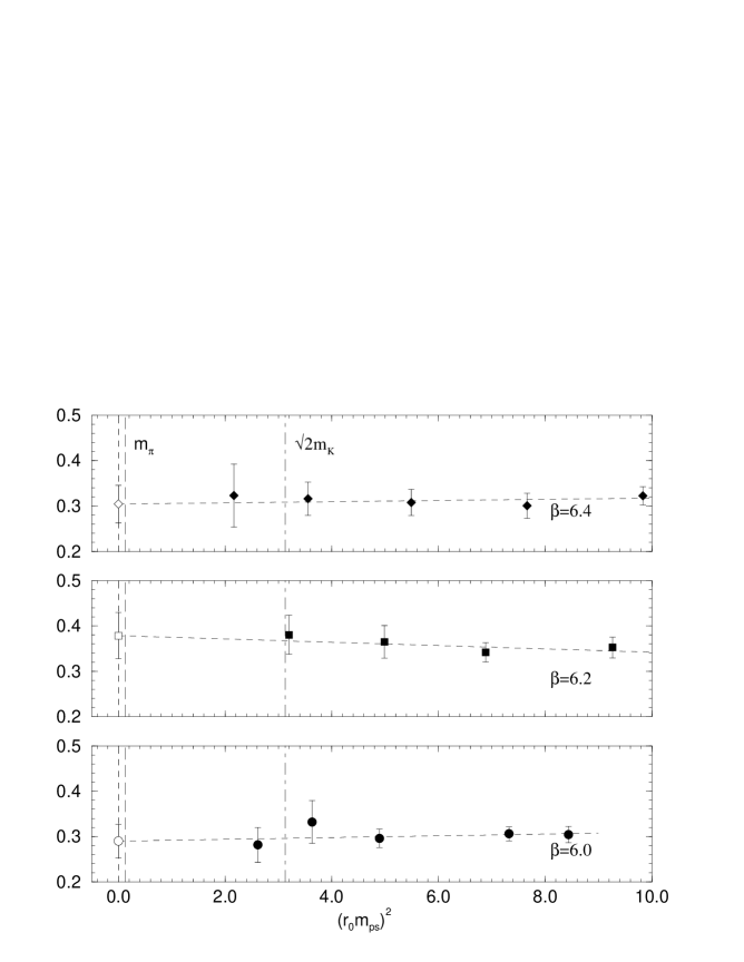
Figure 15: $v^{\mbox{\tiny$R\!G\!I$}}_{2a}$ versus $(r_{0}m_{ps})^{2}$ for $\beta=6.0$ (circles), $6.2$ (squares) and $6.4$ (diamonds). Also shown are linear extrapolations to the chiral limit (dashed lines). Other notation as in Fig. 6.

we show the results for $v_{2a}$ for $\beta=6.0$, $6.2$ and $6.4$ together with a linear chiral extrapolation (using the TI value for $c_{0}$). Immediately noticeable when comparing with Fig. 14 is the large increase in the error bars and less consistent ordering of gradients with increasing $\beta$.

In Fig. 16 we show the results for

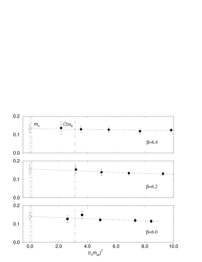
Figure 16: $v^{\mbox{\tiny$R\!G\!I$}}_{3}$ versus $(r_{0}m_{ps})^{2}$ for $\beta=6.0$ (circles), $6.2$ (squares) and $6.4$ (diamonds). Also shown are linear extrapolations to the chiral limit (dashed lines). Other notation as in Fig. 6.

$v_{3}$ and in Fig. 17

Figure 17: $v^{\mbox{\tiny$R\!G\!I$}}_{4}$ versus $(r_{0}m_{ps})^{2}$ for $\beta=6.0$ (circles), $6.2$ (squares) and $6.4$ (diamonds). Also shown are linear extrapolations to the chiral limit (dashed lines). Other notation as in Fig. 6.

the analogous results for $v_{4}$. As expected the results become noisier for increasing $\beta$. Perhaps surprisingly the results for $v_{4}$ seem to be as consistent over our $\beta$-range as those of $v_{3}$ (we have no real explanation for this).

The last limit to be taken is the continuum limit, $a\to 0$. As discussed in section 4 we believe that for $v_{2}$ the improvement terms are numerically small and so can be neglected. Thus we can make an extrapolation in $a^{2}$ (rather than $a$). While we cannot be so confident in this for the higher moments, based on the experience with the lowest moment, we shall also assume this for these higher moments. In Table 5 we give first the RGI values

$\beta$	$\vec{p}$	$6.0$	$6.2$	$6.4$	$\infty$
$v^{\mbox{\tiny$R\!G\!I$}}_{2a}$	$\vec{p}_{1}$	0.290(37)	0.379(51)	0.304(41)	0.343(56)
$v^{\mbox{\tiny$R\!G\!I$}}_{2b}$	$\vec{p}_{1}$	0.338(16)	0.328(16)	0.340(16)	0.335(22)
$v^{\mbox{\tiny$R\!G\!I$}}_{2b}$	$\vec{0}$	0.354(8)	0.344(8)	0.342(8)	0.335(11)
$v^{\mbox{\tiny$R\!G\!I$}}_{3}$	$\vec{p}_{1}$	0.141(19)	0.156(24)	0.132(20)	0.137(28)
$v^{\mbox{\tiny$R\!G\!I$}}_{4}$	$\vec{p}_{1}$	0.090(14)	0.099(29)	0.104(26)	0.110(33)

Table 5: $v^{\mbox{\tiny$R\!G\!I$}}_{n}$ results for $O(a)$ improved fermions at $\beta=6.0$, $6.2$ and $6.4$, for $v^{\mbox{\tiny$R\!G\!I$}}_{n}$, $n=2$, $3$ and $4$. ‘$\infty$’ denotes the continuum extrapolation ($a=0$) limit.

at $\beta=6.0$, $6.2$, $6.4$, for $v^{\mbox{\tiny$R\!G\!I$}}_{2a}$, $v^{\mbox{\tiny$R\!G\!I$}}_{2b}$ both for non-zero and zero momentum, $v^{\mbox{\tiny$R\!G\!I$}}_{3}$ and $v^{\mbox{\tiny$R\!G\!I$}}_{4}$. (These have all been obtained using the NP method II results, as given in Table 4.)

We now use these results to perform a continuum extrapolation. In Fig. 18

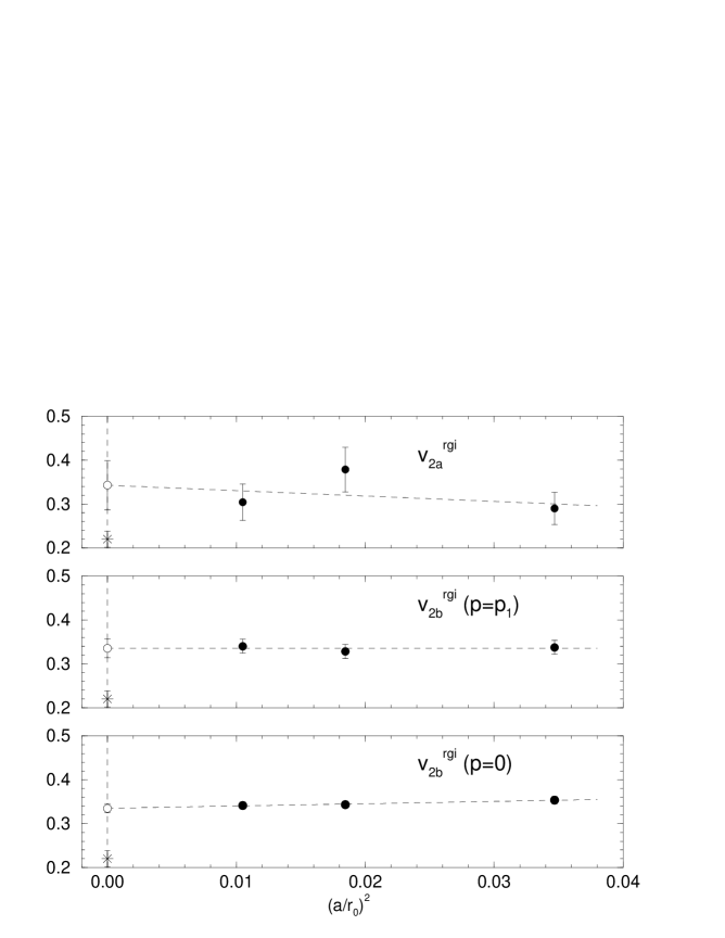
Figure 18: $v^{\mbox{\tiny$R\!G\!I$}}_{2a}$ and $v^{\mbox{\tiny$R\!G\!I$}}_{2b}$ (both for $\vec{p}=\vec{p}_{1}$ and $\vec{0}$) versus $(a/r_{0})^{2}$, using the results at $\beta=6.0$, $6.2$, $6.4$ (filled circles). A linear continuum extrapolation in $a^{2}$ is also given (dashed line and empty circle). The star is the MRST value given in Table 1.

we plot the continuum extrapolations for the various $v^{\mbox{\tiny$R\!G\!I$}}_{2}$. A very consistent picture is obtained firstly between the different representations (‘$a$’ and ‘$b$’) and secondly between the different momenta used in the ‘$b$’ representation. As expected though using a non-zero momentum gives a much noisier signal: in the extreme case between the off-diagonal and diagonal representations the error is about $\sim O(2)$ larger. We shall present our final result using $v^{\mbox{\tiny$R\!G\!I$}}_{2b}$ for $\vec{p}=\vec{0}$ only. In Fig. 19

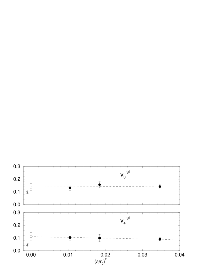
Figure 19: $v^{\mbox{\tiny$R\!G\!I$}}_{3}$ and $v^{\mbox{\tiny$R\!G\!I$}}_{4}$ versus $(a/r_{0})^{2}$, using the results at $\beta=6.0$, $6.2$, $6.4$. A continuum extrapolation is also given. The same notation as for Fig. 18.

we show the results for $v^{\mbox{\tiny$R\!G\!I$}}_{3}$ and $v^{\mbox{\tiny$R\!G\!I$}}_{4}$. Using the modified operators of eq. (33) enables a relatively smooth extrapolation to the continuum limit, giving results with about a $20\%$ – $30\%$ error.

Finally, we convert our results to the $\overline{MS}$ scheme at a scale of $\mu=2\,\mbox{GeV}$, using the three loop result for $[\Delta Z_{v_{n}}^{\mbox{\tiny$\overline{MS}$}}(\mu)]^{-1}$ given in Table 6. We find

$$v_{2}^{\mbox{\tiny$\overline{MS}$}}(2\,\mbox{GeV}) = 0.245(9)\,,$$

$$v_{3}^{\mbox{\tiny$\overline{MS}$}}(2\,\mbox{GeV}) = 0.083(17)\,,$$

$$v_{4}^{\mbox{\tiny$\overline{MS}$}}(2\,\mbox{GeV}) = 0.059(18)\,.$$ (79)

The total error are the combined errors from the three point functions and chiral/continuum fits together with the error for the renormalisation constant. For $v_{2b}$ this indicates that the dominant error is now possibly coming from the renormalisation constant; the opposite is so for the higher moments.

How reasonable are the results in comparison with experiment or the MRST phenomenological fits? The MRST numbers from section 3 in Table 1 are also plotted in Figs. 18 and 19. We see that for $v_{2b}^{\mbox{\tiny$R\!G\!I$}}$, the discrepancy between the experimental result and the lattice result stubbornly remains - and has persisted ever since the first pioneering works in the field [1]. It is also notable that $v_{4}^{\mbox{\tiny$R\!G\!I$}}$ in particular is too large in comparison with the phenomenological result. For both $v_{3}^{\mbox{\tiny$R\!G\!I$}}$ and $v_{4}^{\mbox{\tiny$R\!G\!I$}}$ the chiral and continuum extrapolations are more problematic than for $v_{2b}$. This can probably only be resolved by increasing the statistic of the ensembles and by additional simulations at other $\beta$ values.

Finally for completeness we give the results for $v_{n}^{(q)\mbox{\tiny$\overline{MS}$}}$ for $q=u$, $d$ separately. We find

$$v_{2}^{(u)\mbox{\tiny$\overline{MS}$}}(2\,\mbox{GeV}) = 0.436(18)\,,$$

$$v_{3}^{(u)\mbox{\tiny$\overline{MS}$}}(2\,\mbox{GeV}) = 0.136(25)\,,$$

$$v_{4}^{(u)\mbox{\tiny$\overline{MS}$}}(2\,\mbox{GeV}) = 0.096(25)\,,$$ (80)

for the $u$ quark and

$$v_{2}^{(d)\mbox{\tiny$\overline{MS}$}}(2\,\mbox{GeV}) = 0.191(7)\,,$$

$$v_{3}^{(d)\mbox{\tiny$\overline{MS}$}}(2\,\mbox{GeV}) = 0.052(11)\,,$$

$$v_{4}^{(d)\mbox{\tiny$\overline{MS}$}}(2\,\mbox{GeV}) = 0.027(15)\,,$$ (81)

for the $d$ quark. As discussed previously in section 4.3, the quark line disconnected ($qldis$) contribution to the matrix element is not computed. Thus on the RHS of eqs. (80), (81) there should be an extra term $v_{n}^{\mbox{\tiny$\overline{MS}$}}|_{qldis}$, which is the same for $u$ and $d$ quarks, and of course, cancels for the NS results of eq. (79).

6.2 Chiral perturbation theory

Although linear extrapolations in $m_{ps}^{2}$ seem to describe the results presented earlier quite well, it is not clear that for the quark masses used here (and in other simulations) higher order effects and/or chiral logarithms can be neglected. There has recently been a flurry of interest in this direction. In [5], based on chiral perturbation theory proposed in [4], a fit function model is used which tries to take into account the ‘pion cloud’ around the nucleon, giving with $v^{\mbox{\tiny$R\!G\!I$}}_{n}\equiv F_{\chi}^{(n)}(r_{0}m_{ps})$,

$$F_{\chi}^{(n)}(x) = a_{n}x^{2}+b_{n}\left(1-cx^{2}\ln{x^{2}\over(x^{2}+(r_{0}\Lambda_{\chi})^{2})}\right),$$ (82)

where $\Lambda_{\chi}$ is a parameter, the chiral scale, usually taken to be of $O(4\pi f_{\pi})\sim O(1\,\mbox{GeV})$ (where $f_{\pi}\approx 93\,\mbox{MeV}$). For $\Lambda_{\chi}=0$ or large pseudoscalar mass the equation reduces to the linear case, eq. (78). (Unfortunately as most of the masses used in the present simulation are larger than the strange quark mass, eq. (82) may need higher order terms in chiral perturbation theory to be valid at these large masses.) These first results have been confirmed by further chiral perturbation computations, [6, 7, 8, 9]. In particular in [9], quenched QCD was considered, with the result that at least for the nucleon there are no additional quenched chiral logarithms present, so-called ‘hairpin diagrams’, so the structure of the result in eq. (82) remains unchanged. Furthermore in (unquenched) QCD we have

$$c\equiv{3g_{A}^{2}+1\over(4\pi r_{0}f_{\pi})^{2}}\sim 0.66\,,$$ (83)

while for quenched QCD, assuming that $\alpha^{(2)}\sim\alpha^{(1)}$, $\beta^{(2)}\sim\beta^{(1)}$ in [9], then $c\sim 0.28$. Of course, in principle these formulae, eq. (82), are valid in the continuum so we should first take the continuum limit and then apply chiral perturbation theory. Thus we should interpolate the values for $v_{n}$ in Figs. 14, 15, 16 and 17 to a set of constant $(r_{0}m_{ps})^{2}$ for each value of $\beta$. For each of these values of $(r_{0}m_{ps})^{2}$ a continuum extrapolation should be performed. A chiral extrapolation of the data can then be attempted. Unfortunately our ‘grid’ of data points is not fine enough and also for the higher moments is too noisy for this precedure. Thus we shall try a ‘half way house’ approach and attempt a simultaneous continuum and chiral extrapolation of the data,

$$v_{n}^{\mbox{\tiny$R\!G\!I$}}=F^{(n)}_{\chi}(r_{0}m_{ps})+c_{n}\left({a\over r_{0}}\right)^{2}+d_{n}ar_{0}m_{ps}^{2}\,,$$ (84)

where the first term represents chiral physics, given by eq. (78) or eq. (82), the second term discretisation effects and the last term accounts for residual $O(a)$ effects $\propto am_{q}$, see eq. (37). With this type of fit the number of free parameters is slightly reduced in comparison with the previous fit procedure given in section 6.1 and so tends to produce smaller error bars. We shall restrict our results here to our best data set – $v^{\mbox{\tiny$R\!G\!I$}}_{2b}$ and first check that using eq. (78) for $F^{(2)}_{\chi}$ reproduces our previous results. In Fig. 20

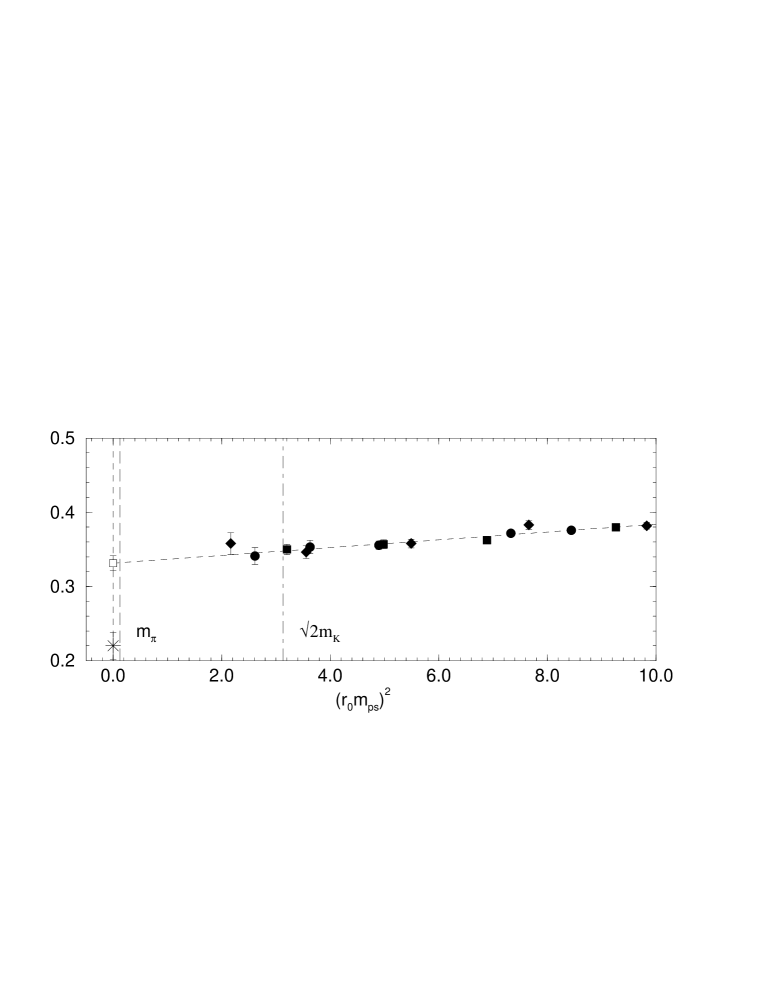
Figure 20: $v^{\mbox{\tiny$R\!G\!I$}}_{2b}-c_{2}(a/r_{0})^{2}-d_{2}ar_{0}m_{ps}^{2}\equiv F^{(2)}_{\chi}=a_{2}(r_{0}m_{ps})^{2}+b_{2}$ (ie using the chiral function of eq. (78)) versus $(r_{0}m_{ps})^{2}$, dashed line. Filled circles, squares and diamonds represent $\beta=6.0$, $6.2$ and $6.4$ respectively. The empty square represents the chirally extrapolated value. Again the MRST phenomenological value of $v^{\mbox{\tiny$R\!G\!I$}}_{2}$ is represented by a star.

we first fit $v^{\mbox{\tiny$R\!G\!I$}}_{2b}$ to eq. (84) with $F^{(2)}_{\chi}$ given by the linear function of eq. (78), $F^{(2)}_{\chi}=a_{2}(r_{0}m_{ps})^{2}+b_{2}$, and then plot $v^{\mbox{\tiny$R\!G\!I$}}_{2b}-c_{2}(a/r_{0})^{2}-d_{2}ar_{0}m_{ps}^{2}$ for our three $\beta$ values. (There is no perceptible difference between using $c_{0}=c_{0}^{\mbox{\tiny$T\!I$}}$ or $c_{0}=0$, for definiteness we show the result for $c_{0}=0$.) The points lie reasonably well on a straight line, with extrapolated result $0.331(10)$ consistent with our previously obtained value in Table 5. The alternative possibility of $v_{2}^{\mbox{\tiny$R\!G\!I$}}-(F_{\chi}^{(2)}(r_{0}m_{ps})-d_{2}ar_{0}m_{ps}^{2})$ versus $(a/r_{0})^{2}$ would display the $O(a^{2})$ lattice discretisation errors. However from Fig. 18 we see that the $O(a^{2})$ effects are small and this alternative plot just reproduces them again.

Bolstered by this result, we now try to use $F_{\chi}^{(2)}$ from eq. (82) as shown in Fig. 21.

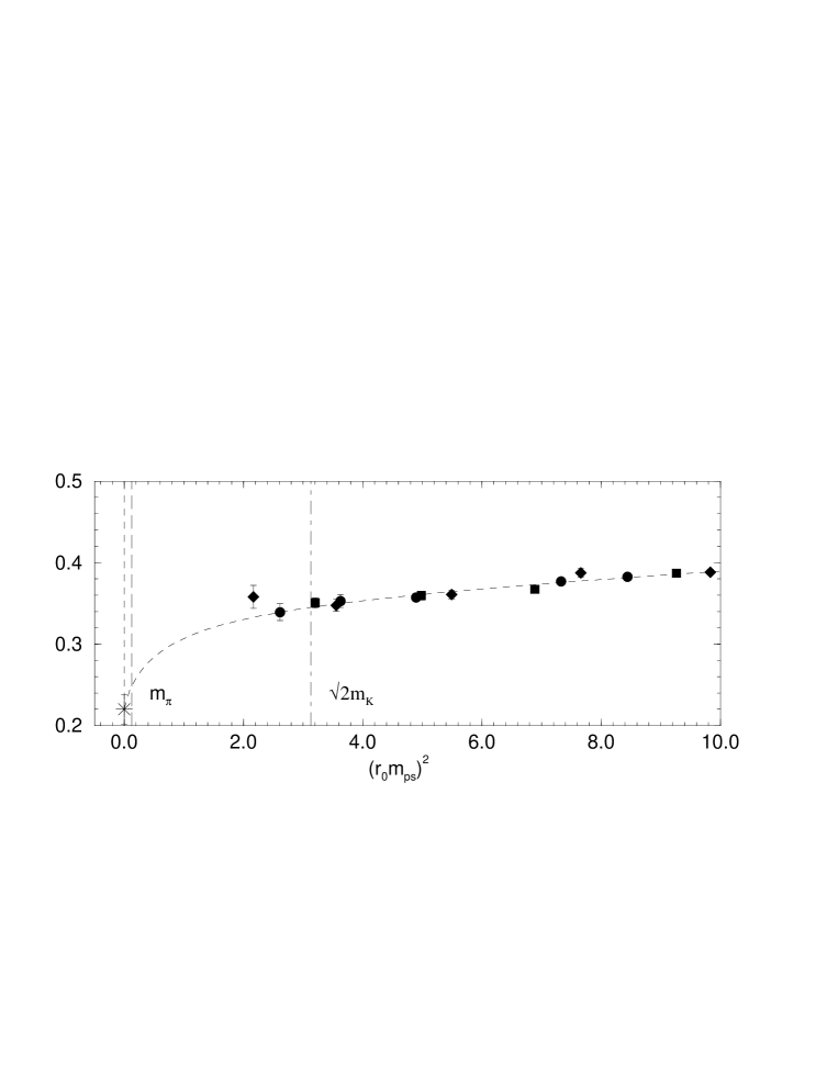
Figure 21: $v^{\mbox{\tiny$R\!G\!I$}}_{2b}-c_{2}(a/r_{0})^{2}-d_{2}ar_{0}m_{ps}^{2}\equiv F^{(2)}_{\chi}$ (using the chiral function of eq. (82)) versus $(r_{0}m_{ps})^{2}$, dashed line. The chiral limit was fixed to the MRST phenomenological value. Other notation is the same as in Fig. 20.

However it is difficult to detect any non-linearities in the data and a $6$-parameter fit ($a_{2}$, $b_{2}$, $c$, $\Lambda_{\chi}$, $c_{2}$, $d_{2}$) fails. We were forced to see if such a 6-parameter fit could be plausible, by fixing the chiral limit, $b_{2}$ to be the MRST phenomenological value given in Table 1. (Note that there is no reason that the quenched QCD value must be the same as the QCD value, however for many hadronic quantities there appears to be little difference between the quenched and unquenched QCD values.) As expected, while the fit (dashed) line and the numerical results are in reasonable agreement, all of the curvature of the fit takes place at small quark mass values where there is no data. Also the fitted parameter result for the chiral scale, $\Lambda_{\chi}\sim 505(48)\,\mbox{MeV}$, is small in comparison with the expected value discussed earlier. For $c$ we found $0.39(6)$ which lies between the unquenched and quenched values.

So it would seem that any possible non-linearities can only show up at rather small quark mass outside the present range of data. Teraflop simulations will be necessary to reach more physical pion masses. At present we shall stick to the simplest extrapolation possible.

7 Conclusions

In this article we have computed $v_{n}$, $n=2,3,4$. There is still a difference between the lattice results and the phenomenological results, particularly apparent for $v_{2}$ where there is a $\sim 40\%$ discrepancy.

We have tried here to narrow down the range of possibilities for the disagreement, on the experimental side by comparing the global MRST/CTEQ fits with the experimental data: there is good agreement.

On the lattice side, we have $O(a)$ improved the lowest moment, investigated possible mixing operators for the higher moments and discussed renormalisation, both perturbatively and non-perturbatively. At least for $v_{2}$ there do not seem to be large $O(a^{2})$ corrections and so a continuum extrapolation can be reliably performed. For the higher moments, we have introduced modified operators for $v_{3}$, $v_{4}$, which reduces the numerical noise and improves the signal. It is difficult to see if there are any $O(a)$ corrections. However at present the simplest assumption that these corrections are small also fits with the data.

Although this is only a partial study here of mixing operators for the higher operators (due in part to the present difficulty of even defining renormalisation constants for several of these operators) presently we find little sign of problems. Indeed even for $v_{4}^{m_{3}}$ the mixing with a lower dimensional operator appears harmless. In other situations this is not the case and there may be significant changes, see eg [57].

We have discussed and compared various renormalisation procedures ranging from simple perturbation theory to TRB perturbation theory to a non-perturbative method. Using NP results eliminates uncertainty concerning the renormalisation constant. It is seen though that between TRB perturbation theory and non-perturbative results there can be up to an $8\%$ difference – far less than the difference between the lattice and phenomenological result for $v_{2}^{\mbox{\tiny$R\!G\!I$}}$.

Finally although at present we see little numerical evidence of chiral logarithms, this is perhaps telling us that we must go to significantly smaller quark masses before the chiral extrapolation ‘bends’ over. However preliminary results at lighter quark mass for unimproved Wilson fermions also show a linear behaviour and so do not seem to improve the situation, [56, 58].

Whether quenching effects are significant remains unclear, but recent unquenched results, [58, 59], do not seem to reveal any significant differences between quenching and unquenching, at least in the quark mass range considered. Finally there are hints of a different situation for overlap fermions, [60], which might suggest again that one has to simulate at light quark masses close to the chiral limit – a challenge for the lattice.

Appendices

Appendix A Some values of $[\Delta Z_{v_{n}}^{\mbox{\tiny$\overline{MS}$}}(\mu)]^{-1}$

$\mu$	one-loop	two-loop	three-loop
	$[\Delta Z_{v_{2}}^{\mbox{\tiny$\overline{MS}$}}(\mu)]^{-1}$
$2.00\,\mbox{GeV}$	$0.783(10)$	$0.721(8)$	$0.732(9)$
$2.12\,\mbox{GeV}$ ($1/a$ at $\beta=6.0$)	$0.776(10)$	$0.715(8)$	$0.726(8)$
$2.90\,\mbox{GeV}$ ($1/a$ at $\beta=6.2$)	$0.743(8)$	$0.688(7)$	$0.696(7)$
$3.85\,\mbox{GeV}$ ($1/a$ at $\beta=6.4$)	$0.718(7)$	$0.668(6)$	$0.674(6)$
	$[\Delta Z_{v_{3}}^{\mbox{\tiny$\overline{MS}$}}(\mu)]^{-1}$
$2.00\,\mbox{GeV}$	$0.682(14)$	$0.596(10)$	$0.609(11)$
$2.12\,\mbox{GeV}$ ($1/a$ at $\beta=6.0$)	$0.673(13)$	$0.589(10)$	$0.602(10)$
$2.90\,\mbox{GeV}$ ($1/a$ at $\beta=6.2$)	$0.629(11)$	$0.555(8)$	$0.564(8)$
$3.85\,\mbox{GeV}$ ($1/a$ at $\beta=6.4$)	$0.596(9)$	$0.529(7)$	$0.537(7)$
	$[\Delta Z_{v_{4}}^{\mbox{\tiny$\overline{MS}$}}(\mu)]^{-1}$
$2.00\,\mbox{GeV}$	$0.619(15)$	$0.520(11)$	$0.534(13)$
$2.12\,\mbox{GeV}$ ($1/a$ at $\beta=6.0$)	$0.609(15)$	$0.512(10)$	$0.526(12)$
$2.90\,\mbox{GeV}$ ($1/a$ at $\beta=6.2$)	$0.559(12)$	$0.476(9)$	$0.486(10)$
$3.85\,\mbox{GeV}$ ($1/a$ at $\beta=6.4$)	$0.522(10)$	$0.448(8)$	$0.456(8)$
	$\alpha_{s}^{\mbox{\tiny$\overline{MS}$}}(\mu)$
$2.00\,\mbox{GeV}$	$0.268(10)$	$0.195(6)$	$0.201(6)$
$2.12\,\mbox{GeV}$ ($1/a$ at $\beta=6.0$)	$0.261(9)$	$0.191(5)$	$0.196(6)$
$2.90\,\mbox{GeV}$ ($1/a$ at $\beta=6.2$)	$0.228(7)$	$0.170(5)$	$0.174(5)$
$3.85\,\mbox{GeV}$ ($1/a$ at $\beta=6.4$)	$0.205(6)$	$0.156(3)$	$0.159(4)$

Table 6: Useful values of $[\Delta Z_{v_{n}}^{\mbox{\tiny$\overline{MS}$}}(\mu)]^{-1}$ ($n=2$, $3$, $4$) and $\alpha_{s}^{\mbox{\tiny$\overline{MS}$}}(\mu)\equiv(g^{\mbox{\tiny$\overline{MS}$}}(\mu))^{2}/4\pi$. The errors are a reflection of the error in $\Lambda^{\mbox{\tiny$\overline{MS}$}}r_{0}$. The lattice simulations performed here, as described in section 4, give the above $1/a$ values (found from using $r_{0}/a$ in [38], namely $r_{0}/a=5.37$, $7.36$, $9.76$ at $\beta=6.0$, $6.2$, $6.4$ respectively, together with the scale $r_{0}=0.5\,\mbox{fm}$).

Appendix B Group properties of mixing operators - an example

When QCD is put on the lattice, the necessary analytic continuation from Minkowski to Euclidean space replaces the Lorentz group by the orthogonal group $O(4)$, which by the discretisation of space-time is further reduced to the hypercubic group $H(4)\subset O(4)$. Since $H(4)$ is only a finite group, the restrictions imposed by symmetry are less stringent than in the continuum and the possibilities for mixing increase, sometimes in a way which is not easily anticipated by our (continuum) intuition. In this appendix we illustrate the problem by an example. For a more complete and systematic treatment we refer to [33].

As a further symmetry we have charge conjugation. It operates on the fermion fields $q(x)$, $\overline{q}(x)$ and on the lattice gauge field $U_{\mu}(x)$ according to

$$q(x) \stackrel{{\scriptstyle C}}{{\to}} C\overline{q}(x)^{T}\,,$$

$$\overline{q}(x) \stackrel{{\scriptstyle C}}{{\to}} -q(x)^{T}C^{-1}\,,$$

$$U_{\mu}(x) \stackrel{{\scriptstyle C}}{{\to}} U_{\mu}(x)^{*}$$ (85)

with the charge conjugation matrix $C$ satisfying

$$C\gamma_{\mu}^{T}C^{-1}=-\gamma_{\mu}\,.$$ (86)

So we get, eg,

$${\mathcal{O}}^{\gamma}_{\mu_{1}\mu_{2}\ldots\mu_{n}}\stackrel{{\scriptstyle C}}{{\to}}(-1)^{n}{\mathcal{O}}^{\gamma}_{\mu_{1}\mu_{n}\mu_{n-1}\ldots\mu_{2}}\,,$$

$${\mathcal{O}}^{\gamma\gamma_{5}}_{\mu_{1}\mu_{2}\ldots\mu_{n}}\stackrel{{\scriptstyle C}}{{\to}}(-1)^{n-1}{\mathcal{O}}^{\gamma\gamma_{5}}_{\mu_{1}\mu_{n}\mu_{n-1}\ldots\mu_{2}}\,.$$ (87)

Identifying elements $R$ of $H(4)$ with the corresponding $4\times 4$ matrices in the defining representation we find that $R$ acts on $\overline{q}\gamma_{\mu}q$ as follows:

$$\overline{q}\gamma_{\mu}q\stackrel{{\scriptstyle R}}{{\to}}\sum_{\nu}R_{\nu\mu}\bar{q}\gamma_{\nu}q\,,$$ (88)

ie, the four operators $\overline{q}\gamma_{\mu}q$ form a basis for the defining representation of $H(4)$. More generally, we get for the action of $R$:

$${\mathcal{O}}^{\gamma}_{\mu_{1}\mu_{2}\ldots\mu_{n}}\stackrel{{\scriptstyle R}}{{\to}}\sum_{\nu_{1},\nu_{2},\ldots,\nu_{n}}R_{\nu_{1}\mu_{1}}R_{\nu_{2}\mu_{2}}\cdots R_{\nu_{n}\mu_{n}}{\mathcal{O}}^{\gamma}_{\nu_{1}\nu_{2}\ldots\nu_{n}}$$ (89)

and

$${\mathcal{O}}^{\gamma\gamma_{5}}_{\mu_{1}\mu_{2}\ldots\mu_{n}}\stackrel{{\scriptstyle R}}{{\to}}\;\det R\sum_{\nu_{1},\nu_{2},\ldots,\nu_{n}}R_{\nu_{1}\mu_{1}}R_{\nu_{2}\mu_{2}}\cdots R_{\nu_{n}\mu_{n}}{\mathcal{O}}^{\gamma\gamma_{5}}_{\nu_{1}\nu_{2}\ldots\nu_{n}}\,.$$ (90)

Thus the $4^{n}$ operators ${\mathcal{O}}^{\gamma}_{\mu_{1}\mu_{2}\ldots\mu_{n}}$ as well as the operators ${\mathcal{O}}^{\gamma\gamma_{5}}_{\mu_{1}\mu_{2}\ldots\mu_{n}}$ form a basis for a representation of $H(4)$, which for $n>1$ is reducible. It is helpful to consider these operators as forming an orthonormal basis of the representation space. (Orthonormal) bases of irreducible subspaces have been given in [33].

Operators transforming according to the same irreducible representation of $H(4)$ (and having the same ${\cal C}$-parity) will in general mix with each other so that one has to consider appropriate linear combinations. Writing down these linear combinations one has to choose the bases in the different (equivalent) representation spaces such that they transform identically under $H(4)$ and not just equivalently.

Consider two bases which are known to transform according to the same irreducible representation. In order to check whether they even transform identically it is sufficient to compare their transformation behaviour under a set of generators. For $H(4)$ there is a set of three generators $\{\alpha,\beta,\gamma\}$ given by

$$\alpha = \left(\begin{array}[]{cccc}0&1&0&0\\ 1&0&0&0\\ 0&0&1&0\\ 0&0&0&1\end{array}\right)\,,$$ (95)

$$\beta = \left(\begin{array}[]{cccc}0&0&0&1\\ 1&0&0&0\\ 0&1&0&0\\ 0&0&1&0\end{array}\right)\,,$$ (100)

$$\gamma = \left(\begin{array}[]{cccc}-1&0&0&0\\ 0&1&0&0\\ 0&0&1&0\\ 0&0&0&1\end{array}\right)\,.$$ (105)

According to (89), $\alpha$ interchanges 1 and 2, $\beta$ performs a cyclic permutation of the values of the indices, and $\gamma$ produces a factor of $-1$ for every index 1, eg, for the operator ${\mathcal{O}}^{\gamma}_{3341}$ one finds

$${\mathcal{O}}^{\gamma}_{3341} \stackrel{{\scriptstyle\alpha}}{{\to}} {\mathcal{O}}^{\gamma}_{3342}\,,$$

$${\mathcal{O}}^{\gamma}_{3341} \stackrel{{\scriptstyle\beta}}{{\to}} {\mathcal{O}}^{\gamma}_{4412}\,,$$

$${\mathcal{O}}^{\gamma}_{3341} \stackrel{{\scriptstyle\gamma}}{{\to}} -{\mathcal{O}}^{\gamma}_{3341}\,.$$ (106)

As an example for mixing operators, let us consider $\mathcal{O}_{v_{4}}$. It belongs to a doublet of operators transforming according to the $H(4)$ representation $\tau^{(2)}_{1}$ (in the notation of [55] and Table 2) and has positive ${\cal C}$-parity. Indeed, the two operators

$$u_{1}:=\frac{\sqrt{6}}{2}\left({\mathcal{O}}^{\gamma}_{\{1122\}}+{\mathcal{O}}^{\gamma}_{\{3344\}}-{\mathcal{O}}^{\gamma}_{\{1133\}}-{\mathcal{O}}^{\gamma}_{\{2244\}}\right)\,,$$ (107)

and

$$u_{2}:=\frac{1}{\sqrt{2}}\left(2{\mathcal{O}}^{\gamma}_{\{1144\}}+2{\mathcal{O}}^{\gamma}_{\{2233\}}-{\mathcal{O}}^{\gamma}_{\{1122\}}-{\mathcal{O}}^{\gamma}_{\{3344\}}-{\mathcal{O}}^{\gamma}_{\{1133\}}-{\mathcal{O}}^{\gamma}_{\{2244\}}\right)=\sqrt{2}\mathcal{O}_{v_{4}}$$ (108)

form an orthonormal basis for this representation. It is obvious that both operators remain unchanged under the action of $\gamma$. The generator $\alpha$ acts on them as follows:

$$u_{1} \stackrel{{\scriptstyle\alpha}}{{\to}} \mbox{\small$\frac{1}{2}$}u_{1}-\mbox{\small$\frac{1}{2}$}\sqrt{3}u_{2}\,,$$

$$u_{2} \stackrel{{\scriptstyle\alpha}}{{\to}} -\mbox{\small$\frac{1}{2}$}\sqrt{3}u_{1}-\mbox{\small$\frac{1}{2}$}u_{2}\,,$$ (109)

while $\beta$ gives

$$u_{1} \stackrel{{\scriptstyle\beta}}{{\to}} \mbox{\small$\frac{1}{2}$}u_{1}+\mbox{\small$\frac{1}{2}$}\sqrt{3}u_{2}\,,$$

$$u_{2} \stackrel{{\scriptstyle\beta}}{{\to}} \mbox{\small$\frac{1}{2}$}\sqrt{3}u_{1}-\mbox{\small$\frac{1}{2}$}u_{2}\,.$$ (110)

It is straightforward to check that the operators

$$w_{1} := \frac{1}{4\sqrt{3}}\Big{(}{}-{\mathcal{O}}^{\gamma}_{1122}-{\mathcal{O}}^{\gamma}_{2112}-{\mathcal{O}}^{\gamma}_{1221}-{\mathcal{O}}^{\gamma}_{2211}+2{\mathcal{O}}^{\gamma}_{1212}+2{\mathcal{O}}^{\gamma}_{2121}$$ (111)

$$\hphantom{\frac{1}{4\sqrt{3}}\Big{(}}{}-{\mathcal{O}}^{\gamma}_{3344}-{\mathcal{O}}^{\gamma}_{4334}-{\mathcal{O}}^{\gamma}_{3443}-{\mathcal{O}}^{\gamma}_{4433}+2{\mathcal{O}}^{\gamma}_{3434}+2{\mathcal{O}}^{\gamma}_{4343}$$

$$\hphantom{\frac{1}{4\sqrt{3}}\Big{(}}{}+{\mathcal{O}}^{\gamma}_{1133}+{\mathcal{O}}^{\gamma}_{3113}+{\mathcal{O}}^{\gamma}_{1331}+{\mathcal{O}}^{\gamma}_{3311}-2{\mathcal{O}}^{\gamma}_{1313}-2{\mathcal{O}}^{\gamma}_{3131}$$

$$\hphantom{\frac{1}{4\sqrt{3}}\Big{(}}{}+{\mathcal{O}}^{\gamma}_{2244}+{\mathcal{O}}^{\gamma}_{4224}+{\mathcal{O}}^{\gamma}_{2442}+{\mathcal{O}}^{\gamma}_{4422}-2{\mathcal{O}}^{\gamma}_{2424}-2{\mathcal{O}}^{\gamma}_{4242}\Big{)}\,,$$

and

$$w_{2} := \frac{1}{12}\Big{(}+{\mathcal{O}}^{\gamma}_{1122}+{\mathcal{O}}^{\gamma}_{2112}+{\mathcal{O}}^{\gamma}_{1221}+{\mathcal{O}}^{\gamma}_{2211}-2{\mathcal{O}}^{\gamma}_{1212}-2{\mathcal{O}}^{\gamma}_{2121}$$ (112)

$$\hphantom{\frac{1}{12}\Big{(}}{}+{\mathcal{O}}^{\gamma}_{3344}+{\mathcal{O}}^{\gamma}_{4334}+{\mathcal{O}}^{\gamma}_{3443}+{\mathcal{O}}^{\gamma}_{4433}-2{\mathcal{O}}^{\gamma}_{3434}-2{\mathcal{O}}^{\gamma}_{4343}$$

$$\hphantom{\frac{1}{12}\Big{(}}{}+{\mathcal{O}}^{\gamma}_{1133}+{\mathcal{O}}^{\gamma}_{3113}+{\mathcal{O}}^{\gamma}_{1331}+{\mathcal{O}}^{\gamma}_{3311}-2{\mathcal{O}}^{\gamma}_{1313}-2{\mathcal{O}}^{\gamma}_{3131}$$

$$\hphantom{\frac{1}{12}\Big{(}}{}+{\mathcal{O}}^{\gamma}_{2244}+{\mathcal{O}}^{\gamma}_{4224}+{\mathcal{O}}^{\gamma}_{2442}+{\mathcal{O}}^{\gamma}_{4422}-2{\mathcal{O}}^{\gamma}_{2424}-2{\mathcal{O}}^{\gamma}_{4242}$$

$$\hphantom{\frac{1}{12}\Big{(}}{}-2{\mathcal{O}}^{\gamma}_{1144}-2{\mathcal{O}}^{\gamma}_{4114}-2{\mathcal{O}}^{\gamma}_{1441}-2{\mathcal{O}}^{\gamma}_{4411}+4{\mathcal{O}}^{\gamma}_{1414}+4{\mathcal{O}}^{\gamma}_{4141}$$

$$\hphantom{\frac{1}{12}\Big{(}}{}-2{\mathcal{O}}^{\gamma}_{2233}-2{\mathcal{O}}^{\gamma}_{3223}-2{\mathcal{O}}^{\gamma}_{2332}-2{\mathcal{O}}^{\gamma}_{3322}+4{\mathcal{O}}^{\gamma}_{2323}+4{\mathcal{O}}^{\gamma}_{3232}\Big{)}\,,$$

$$\hphantom{:}= \frac{1}{6}{\mathcal{O}}^{m_{1}}_{v_{4}}\,,$$

transform identically to $u_{1}$, $u_{2}$:

$$w_{1} \stackrel{{\scriptstyle\alpha}}{{\to}} \mbox{\small$\frac{1}{2}$}w_{1}-\mbox{\small$\frac{1}{2}$}\sqrt{3}w_{2}\,,$$

$$w_{2} \stackrel{{\scriptstyle\alpha}}{{\to}} -\mbox{\small$\frac{1}{2}$}\sqrt{3}w_{1}-\mbox{\small$\frac{1}{2}$}w_{2}\,,$$ (113)

$$w_{1} \stackrel{{\scriptstyle\beta}}{{\to}} \mbox{\small$\frac{1}{2}$}w_{1}+\mbox{\small$\frac{1}{2}$}\sqrt{3}w_{2}\,,$$

$$w_{2} \stackrel{{\scriptstyle\beta}}{{\to}} \mbox{\small$\frac{1}{2}$}\sqrt{3}w_{1}-\mbox{\small$\frac{1}{2}$}w_{2}\,,$$ (114)

and they are invariant under the action of $\gamma$. Hence any linear combination $r\cdot u_{i}+s\cdot w_{i}$ ($i=1,2$) has the same transformation properties under $H(4)$ as $u_{i}$. In particular, ${\mathcal{O}}_{v_{4}}$ may mix with ${\mathcal{O}}^{m_{1}}_{v_{4}}$, and the renormalisation of ${\mathcal{O}}_{v_{4}}$ will in general involve also ${\mathcal{O}}^{m_{1}}_{v_{4}}$.

Also the operators

$$w^{\prime}_{1} := \frac{1}{4}\Big{(}{}+{\mathcal{O}}^{\gamma\gamma_{5}}_{1324}-{\mathcal{O}}^{\gamma\gamma_{5}}_{2314}-{\mathcal{O}}^{\gamma\gamma_{5}}_{1423}+{\mathcal{O}}^{\gamma\gamma_{5}}_{2413}+{\mathcal{O}}^{\gamma\gamma_{5}}_{3142}-{\mathcal{O}}^{\gamma\gamma_{5}}_{4132}-{\mathcal{O}}^{\gamma\gamma_{5}}_{3241}+{\mathcal{O}}^{\gamma\gamma_{5}}_{4231}\hskip 18.06749pt$$ (115)

$${}+{\mathcal{O}}^{\gamma\gamma_{5}}_{1234}-{\mathcal{O}}^{\gamma\gamma_{5}}_{3214}-{\mathcal{O}}^{\gamma\gamma_{5}}_{1432}+{\mathcal{O}}^{\gamma\gamma_{5}}_{3412}+{\mathcal{O}}^{\gamma\gamma_{5}}_{2143}-{\mathcal{O}}^{\gamma\gamma_{5}}_{4123}-{\mathcal{O}}^{\gamma\gamma_{5}}_{2341}+{\mathcal{O}}^{\gamma\gamma_{5}}_{4321}\Big{)}\,,$$

and

$$w^{\prime}_{2} := \frac{1}{4\sqrt{3}}\Big{(}{}+{\mathcal{O}}^{\gamma\gamma_{5}}_{1234}-{\mathcal{O}}^{\gamma\gamma_{5}}_{3214}-{\mathcal{O}}^{\gamma\gamma_{5}}_{1432}+{\mathcal{O}}^{\gamma\gamma_{5}}_{3412}+{\mathcal{O}}^{\gamma\gamma_{5}}_{2143}-{\mathcal{O}}^{\gamma\gamma_{5}}_{4123}-{\mathcal{O}}^{\gamma\gamma_{5}}_{2341}+{\mathcal{O}}^{\gamma\gamma_{5}}_{4321}$$ (116)

$$\hphantom{\frac{1}{4\sqrt{3}}\Big{(}}{}-{\mathcal{O}}^{\gamma\gamma_{5}}_{1324}+{\mathcal{O}}^{\gamma\gamma_{5}}_{2314}+{\mathcal{O}}^{\gamma\gamma_{5}}_{1423}-{\mathcal{O}}^{\gamma\gamma_{5}}_{2413}-{\mathcal{O}}^{\gamma\gamma_{5}}_{3142}+{\mathcal{O}}^{\gamma\gamma_{5}}_{4132}+{\mathcal{O}}^{\gamma\gamma_{5}}_{3241}-{\mathcal{O}}^{\gamma\gamma_{5}}_{4231}$$

$$\hphantom{\frac{1}{4\sqrt{3}}\Big{(}}{}+2{\mathcal{O}}^{\gamma\gamma_{5}}_{1243}-2{\mathcal{O}}^{\gamma\gamma_{5}}_{4213}-2{\mathcal{O}}^{\gamma\gamma_{5}}_{1342}+2{\mathcal{O}}^{\gamma\gamma_{5}}_{4312}+2{\mathcal{O}}^{\gamma\gamma_{5}}_{2134}-2{\mathcal{O}}^{\gamma\gamma_{5}}_{3124}$$

$$\hphantom{\frac{1}{4\sqrt{3}}\Big{(}+2{\mathcal{O}}^{\gamma\gamma_{5}}_{1243}-2{\mathcal{O}}^{\gamma\gamma_{5}}_{4213}-2{\mathcal{O}}^{\gamma\gamma_{5}}_{1342}+2{\mathcal{O}}^{\gamma\gamma_{5}}_{4312}}{}-2{\mathcal{O}}^{\gamma\gamma_{5}}_{2431}+2{\mathcal{O}}^{\gamma\gamma_{5}}_{3421}\Big{)}\,,$$

$$\hphantom{:}= \frac{1}{2\sqrt{3}}{\mathcal{O}}^{m_{2}}_{v_{4}}\,,$$

transform in exactly the same way under $\alpha$, $\beta$, and $\gamma$, ie under $H(4)$, as follows from (90). Therefore ${\mathcal{O}}^{m_{2}}_{v_{4}}$ may mix with ${\mathcal{O}}_{v_{4}}$, too.

Appendix C Two- and three-point correlation functions

C.1 General formulae

In this appendix we shall give explicit expressions for the correlation functions in terms of quark propagators. We start with the two-point correlation function. A suitable proton operator is

$$B_{\alpha}(t;\vec{p})=\sum_{\vec{x}}e^{-i\vec{p}\cdot\vec{x}}\epsilon^{abc}u^{a}_{\alpha}(\vec{x},t)\left[u^{b}(\vec{x},t)^{T_{D}}C\gamma_{5}d^{c}(\vec{x},t)\right]\,,$$ (117)

($a\ldots$ denote colour indices, $\alpha\ldots$ Dirac indices, $T_{D}$ is the transpose in Dirac space and $\gamma_{5}=\gamma_{1}\gamma_{2}\gamma_{3}\gamma_{4}$). $C$, the charge conjugation matrix, has the defining property given in eq. (86) and is antisymmetric. As we take our gamma matrices to be hermitian then $C$ may be taken as as unitary. Thus $-C=C^{T_{D}}$ and $C^{-1}=C^{\dagger}$. One possible choice (used in our computer programme) is $C=\gamma_{4}\gamma_{2}$ (so that $-C=C^{-1}$) and the Dirac basis

$$\gamma_{i}=\left(\begin{array}[c]{cc}0&-i\sigma_{i}\\ i\sigma_{i}&0\end{array}\right)\,,\qquad\gamma_{4}=\left(\begin{array}[c]{cc}I&0\\ 0&-I\end{array}\right)\,,$$ (118)

(but the results given here should not depend on this particular choice). The last two quark fields in eq. (117) form a di-quark structure, while the first quark carries the spin index. With the help of

$$\overline{B}_{\alpha}(t;\vec{p})=\sum_{\vec{x}}e^{i\vec{p}.\vec{x}}\epsilon^{abc}\overline{u}^{a}_{\alpha}(\vec{x},t)\left[\overline{d}^{b}(\vec{x},t)\gamma_{5}C\overline{u}^{c}(\vec{x},t)^{T_{D}}\right]\,,$$ (119)

the two-point correlation function is formed in the usual way

$$C_{\Gamma}(t;\vec{p})=\mbox{Tr}_{D}\Gamma\langle B(t,\vec{p})\overline{B}(0,\vec{p})\rangle\,,$$ (120)

where we have introduced an arbitrary Dirac matrix, $\Gamma$, which for unpolarised nucleons, the case considered here, should be taken as $\mbox{\small$\frac{1}{2}$}(1+\gamma_{4})$. This equation may be re-written using quark propagators propagating from a (point) source to a sink. As we are averaging over the gauge fields we may shift all sources to $(\vec{0},0)$. Some algebra then yields

$$C_{\Gamma}(t;\vec{p})=-V_{s}\sum_{\vec{x}}e^{-i\vec{p}\cdot\vec{x}}\epsilon^{abc}\epsilon^{a^{\prime}b^{\prime}c^{\prime}}$$ (121)

$$\left\langle\mbox{Tr}_{D}\left[\Gamma G^{(u)aa^{\prime}}(\vec{x},t;\vec{0},0)\right]\mbox{Tr}_{D}\left[\tilde{G}^{(d)bb^{\prime}}(\vec{x},t;\vec{0},0)G^{(u)cc^{\prime}}(\vec{x},t;\vec{0},0)\right]\right.$$

$$\qquad\quad+\left.\mbox{Tr}_{D}\left[\Gamma G^{(u)aa^{\prime}}(\vec{x},t;\vec{0},0)\tilde{G}^{(d)bb^{\prime}}(\vec{x},t;\vec{0},0)G^{(u)cc^{\prime}}(\vec{x},t;\vec{0},0)\right]\right\rangle_{\{U\}}\,,$$

where we have defined a tilde in Dirac space by

$$\tilde{X}=(C\gamma_{5}X\gamma_{5}C)^{T_{D}}\,.$$ (122)

The problem is thus reduced to finding the propagator or Green’s function for quark $q$ from a source $(\vec{0},0)$ to $(\vec{x},t)$. In general, the quark propagator from $y$ to $x$ is defined by

$$G^{(q)ab}_{\alpha\beta}(x;y)=\langle{q}_{\alpha}^{a}(x)\overline{{q}}_{\beta}^{b}(y)\rangle_{q}\,,$$ (123)

and can be computed from

$$\sum_{w}M^{(q)}(x;w)G^{(q)}(w;y)=\delta_{xy}\,,\$$ (124)

where $M_{\alpha\beta}^{ab}$ is the Wilson (clover) matrix, given in Appendix D.

For the three-point correlation function,

$$C_{\Gamma}(t,\tau;\vec{p};{\cal O}_{q})=\mbox{Tr}_{D}\Gamma\langle B(t,\vec{p}){\cal O}_{q}(\tau)\overline{B}(0,\vec{p})\rangle\,,$$ (125)

we shall only consider the quark line connected term (ie the left diagram of Fig. 4). First we re-write the operator insertion generally as

$${\cal O}_{q}(\tau) = \sum_{\vec{y}}{\cal O}_{q}(\vec{y},\tau)$$ (126)

$$= \sum_{\vec{y},v,w}\overline{q}^{a}_{\alpha}(v)O_{\alpha\beta}^{ab}(v,w;\vec{y},\tau)q_{\beta}^{b}(w)$$

(ie sum over spatial planes, where $(\vec{y},\tau)$ is the ‘center of mass of the operator’). For operators without derivatives and with exactly one derivative we have $\overline{q}\gamma q$ and $\mbox{\small$\frac{1}{2}$}\overline{q}\gamma(\stackrel{{\scriptstyle\rightarrow}}{{D}}-\stackrel{{\scriptstyle\leftarrow}}{{D}})q$ for ${\cal O}_{q}$ respectively, ($\stackrel{{\scriptstyle\rightarrow}}{{D}}$ and $\stackrel{{\scriptstyle\leftarrow}}{{D}}$ are defined in eq. (32)) while for two and three derivative operators, to minimise the extension on the lattice we ‘integrate by parts’ and choose $-\overline{q}\gamma\stackrel{{\scriptstyle\leftarrow}}{{D}}\stackrel{{\scriptstyle\rightarrow}}{{D}}q$ and $\mbox{\small$\frac{1}{2}$}\overline{q}\gamma(\stackrel{{\scriptstyle\leftarrow}}{{D}}\stackrel{{\scriptstyle\leftarrow}}{{D}}\stackrel{{\scriptstyle\rightarrow}}{{D}}-\stackrel{{\scriptstyle\leftarrow}}{{D}}\stackrel{{\scriptstyle\rightarrow}}{{D}}\stackrel{{\scriptstyle\rightarrow}}{{D}})q$ respectively. This also allows the higher derivative operators to be built from the previously constructed lower derivative operators.

Some algebra yields the result for eq. (125) of

$$C_{\Gamma}(t,\tau;\vec{p};{\cal O}_{q})$$ (127)

$$= -V_{s}\sum_{\vec{y},v,w}\left\langle\mbox{Tr}_{CD}\left[\Sigma_{\Gamma}^{(q)}(\vec{0},0;v;\vec{p},t)O(v,w;\vec{y},\tau)G^{(q)}(w;0,0)\right]\right\rangle_{\{U\}}\,,$$

where $\Sigma_{\Gamma}^{(q)}(\vec{0},0;v;\vec{p},t)$ is given by

$$\Sigma_{\Gamma}^{(q)}(\vec{0},0;v;\vec{p},t)=\sum_{\vec{x}}S_{\Gamma}^{(q)}(\vec{x},t;\vec{0},0;\vec{p})G^{(q)}(\vec{x},t;v)\,,$$ (128)

in terms of

$$S^{(u)a^{\prime}a}_{\Gamma}(\vec{x},t;\vec{0},0;\vec{p})=e^{-i\vec{p}\cdot\vec{x}}\epsilon^{abc}\epsilon^{a^{\prime}b^{\prime}c^{\prime}}\times$$

$$\left[\widetilde{G}^{(d)bb^{\prime}}(\vec{x},t;\vec{0},0)G^{(u)cc^{\prime}}(\vec{x},t;\vec{0},0)\Gamma+\mbox{Tr}_{D}[\widetilde{G}^{(d)bb^{\prime}}(\vec{x},t;\vec{0},0)G^{(u)cc^{\prime}}(\vec{x},t;\vec{0},0)]\Gamma+\right.$$

$$\left.\Gamma G^{(u)bb^{\prime}}(\vec{x},t;\vec{0},0)\widetilde{G}^{(d)cc^{\prime}}(\vec{x},t;\vec{0},0)+\mbox{Tr}_{D}[\Gamma G^{(u)bb^{\prime}}(\vec{x},t;\vec{0},0)]\widetilde{G}^{(d)cc^{\prime}}(\vec{x},t;\vec{0},0)]\right]\,,$$

when $q=u$ and a slightly simpler expression for $S_{\Gamma}^{(d)}$ namely

$$S^{(d)a^{\prime}a}_{\Gamma}(\vec{x},t;\vec{0},0;\vec{p})=e^{-i\vec{p}\cdot\vec{x}}\epsilon^{abc}\epsilon^{a^{\prime}b^{\prime}c^{\prime}}\times$$

$$\left[\widetilde{G}^{(u)bb^{\prime}}(\vec{x},t;\vec{0},0)\widetilde{\Gamma}\widetilde{G}^{(u)cc^{\prime}}(\vec{x},t;\vec{0},0)+\mbox{Tr}_{D}[\Gamma G^{(u)bb^{\prime}}(\vec{x},t;\vec{0},0)\widetilde{G}^{(u)cc^{\prime}}(\vec{x},t;\vec{0},0)]\right]\,.$$

Practically we must find $\Sigma_{\Gamma}^{(q)}$ from a second Green’s function using these rather ugly looking $S_{\Gamma}^{(q)}$ expressions as sources. By considering

$$\sum_{v}\Sigma_{\Gamma}^{(q)}(\vec{0},0;v;\vec{p},t)M^{(q)}(v;v^{\prime})=S_{\Gamma}^{(q)}(\vec{v}^{\,\prime}t;\vec{0},0;\vec{p})\delta_{v_{4}^{\prime}t}\,,$$ (131)

we see that this is the wrong way around for the inversion in eq. (124) but taking colour/spin components and using $M^{ab}_{\alpha\beta}(x;y)=(\gamma_{5}M^{*}(y;x)^{ba}\gamma_{5})_{\beta\alpha}$ the equation for $\Sigma$ can be re-written as

$$\sum_{v}M^{(q)}(v^{\prime};v)\gamma_{5}\Sigma_{\Gamma}^{(q)\dagger_{CD}}(\vec{0},0;v;\vec{p},t)=\gamma_{5}S_{\Gamma}^{(q)\dagger_{CD}}(\vec{v}^{\,\prime},t;\vec{0},0;\vec{p})\delta_{v_{4}^{\prime},t}\,,$$ (132)

where $\dagger_{CD}$ is the Hermitian conjugate in colour and spin space. We see that in this form $\Sigma$ is rather like a Green’s function from the source given on the RHS of the equation.

Thus finding the three point correlation functions is a two step process: first the usual Green’s function from $(\vec{0},0)$ to any point $x$ is found, stage I. Then a second inversion (stage II) is made with the source given from eq. (LABEL:source_u) if the inserted operator consists of $u$ quarks or using eq. (LABEL:source_d) for $d$ quarks.

The advantage of this procedure is that by tying together the two Green’s functions appropriately any operator can be inserted with no additional computational cost. (There is no restriction on the derivative structure and Dirac matrix $\gamma$). The disadvantage is that for each nucleon state (ie $\Gamma$ determining whether the nucleon is unpolarised or polarised), momentum $\vec{p}$ and nucleon sink position ($t$) a separate inversion is required. Thus results for a range of $t$ values are expensive and practically we must restrict ourselves to one value.

C.2 The Non-Relativistic Projection

To improve the overlap with the nucleon we have used Jacobi smearing, [31], and non-relativistic, NR, projection of the nucleon wavefunction. For completeness we now briefly describe our implementation of this projection. Rather than using the nucleon operator of eq. (117) we shall replace it by

$$B^{\mbox{\tiny$N\!R$}}_{\alpha}(t;\vec{p})=\sum_{\vec{x}}e^{-i\vec{p}\cdot\vec{x}}\epsilon^{abc}u^{a}_{\alpha}(\vec{x},t)\left[u^{b}_{\beta}(\vec{x},t)\left(C\gamma_{5}\mbox{\small$\frac{1}{2}$}(1+\gamma_{4})\right)_{\beta\gamma}d_{\gamma}^{c}(\vec{x},t)\right]\,,$$ (133)

ie we replace the matrix $C\gamma_{5}\to C\gamma_{5}\mbox{\small$\frac{1}{2}$}(1+\gamma_{4})$. Both operators (eqs. (133) and (117)) behave the same way under rotations and reflections in the spatial directions, and both have the same quantum numbers (colour neutral, spin $\frac{1}{2}$, isospin $\frac{1}{2}$ and parity $+$), and both will therefore overlap with the proton.

As we shall see, not only is $B^{\mbox{\tiny$N\!R$}}$ computationally cheaper by a factor two, but it has a better overlap with the proton. This can be easiest shown if we use the Dirac basis eq. (118) first giving

$$C\gamma_{5}=\gamma_{4}\gamma_{2}\gamma_{5}=\left(\begin{array}[]{cccc}0&1&0&0\\ -1&0&0&0\\ 0&0&0&1\\ 0&0&-1&0\\ \end{array}\right)\,,\quad C\gamma_{5}\mbox{\small$\frac{1}{2}$}(1+\gamma_{4})=\left(\begin{array}[]{cccc}0&1&0&0\\ -1&0&0&0\\ 0&0&0&0\\ 0&0&0&0\\ \end{array}\right)\,.$$ (134)

If we now write out eq. (133) for a spin-up (ie $\alpha=1$) proton we have

$$B^{\mbox{\tiny$N\!R$}}_{1}=\epsilon^{abc}\left(u^{a}_{1}u^{b}_{1}d^{c}_{2}-u^{a}_{1}u^{b}_{2}d^{c}_{1}\right)\,,$$ (135)

setting $\vec{p}=\vec{0}$ and suppressing the co-ordinate index for simplicity. This is not quite the final form. When we sum over all fermion line diagrams, only the part of the operator which is antisymmetric under the interchange of the two $u$ quarks makes any contribution to the measured Green’s function. Since the colour wavefunction $\epsilon^{abc}$ is completely antisymmetric, this means that the part of eq. (135) which survives is

$$B^{\mbox{\tiny$N\!R$}}_{1}=\epsilon^{abc}\left(u^{a}_{1}u^{b}_{1}d^{c}_{2}-\mbox{\small$\frac{1}{2}$}u^{a}_{1}u^{b}_{2}d^{c}_{1}-\mbox{\small$\frac{1}{2}$}u^{a}_{2}u^{b}_{1}d^{c}_{1}\right)\,.$$ (136)

Since the mid-sixties it has been known that the lowest-lying octet and decuplet baryons are well described as a 56 of $SU(6)$. According to $SU(6)$ the flavour/spin wavefunction of the spin up proton is (eg [61])

$$p_{\uparrow}=\sqrt{\mbox{\small$\frac{1}{6}$}}\left(2u_{\uparrow}u_{\uparrow}d_{\downarrow}-u_{\uparrow}u_{\downarrow}d_{\uparrow}-u_{\downarrow}u_{\uparrow}d_{\uparrow}\right)\,.$$ (137)

Comparing this with eq. (136) we see that this is exactly the wavefunction we have been using. The wavefunction of eq. (137) makes some very successful predictions, for example that the ratio of proton to neutron magnetic moments should be $-\mbox{\small$\frac{3}{2}$}$. The experimental value is $-1.460$, in good agreement with the $SU(6)$ prediction. This success suggests that eq. (136) is close to the true proton wavefunction. We would expect this wavefunction to work even better with heavier quarks, so it is an appropriate wavefunction to use on the lattice. If we carry out the same exercise with eq. (117) we obtain

$$B_{1} = \epsilon^{abc}\big{(}u^{a}_{1}u^{b}_{1}d^{c}_{2}-\mbox{\small$\frac{1}{2}$}u^{a}_{1}u^{b}_{2}d^{c}_{1}-\mbox{\small$\frac{1}{2}$}u^{a}_{2}u^{b}_{1}d^{c}_{1}$$ (138)

$$\hskip 57.81621pt+\mbox{\small$\frac{1}{2}$}u^{a}_{1}u^{b}_{3}d^{c}_{4}+\mbox{\small$\frac{1}{2}$}u^{a}_{3}u^{b}_{1}d^{c}_{4}-\mbox{\small$\frac{1}{2}$}u^{a}_{1}u^{b}_{4}d^{c}_{3}-\mbox{\small$\frac{1}{2}$}u^{a}_{4}u^{b}_{1}d^{c}_{3}\Big{)}\,,$$

as the explicit component expression. This has many terms involving the 3rd and 4th Dirac components with amplitudes just as large as the terms with upper components only. In any sort of constituent quark model we would expect these terms to be small in the ground state. Adding them into the wavefunction not only increases the cost of the computation, it also degrades the signal by adding terms which are likely to have more overlap with excited baryon states.

The correlation functions are constructed also using

$$\overline{B}^{\mbox{\tiny$N\!R$}}_{\alpha}(t;\vec{p})=\sum_{\vec{x}}e^{i\vec{p}.\vec{x}}\epsilon^{abc}\overline{u}^{a}_{\alpha}(\vec{x},t)\left[\overline{d}^{b}(\vec{x},t)\mbox{\small$\frac{1}{2}$}(1+\gamma_{4})\gamma_{5}C\overline{u}^{c}(\vec{x},t)^{T_{D}}\right]\,,$$ (139)

ie replacing $\gamma_{5}C\to\mbox{\small$\frac{1}{2}$}(1+\gamma_{4})\gamma_{5}C$. Thus the NR projection can be obtained by projecting out the positive eigenvalues of $\gamma_{4}$, ie by replacing each quark field, $q$, by

$$q\to\mbox{\small$\frac{1}{2}$}(1+\gamma_{4})q\,,\qquad\overline{q}\to\overline{q}\mbox{\small$\frac{1}{2}$}(1+\gamma_{4})\,,$$ (140)

everywhere and considering polarisation matrices $\Gamma$ which satisfy

$$\mbox{\small$\frac{1}{2}$}(1+\gamma_{4})\Gamma=\Gamma=\Gamma\mbox{\small$\frac{1}{2}$}(1+\gamma_{4})\,.$$ (141)

This gives the NR nucleon two-point function, eq. (120). (So for the Dirac basis, eq. (118), only the components $\alpha=1$, $2$ are non-zero, as discussed above.) In Fig. 22

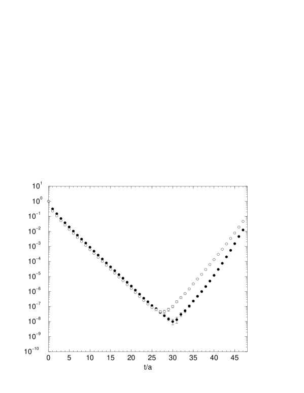
Figure 22: Relativistic (open circles) and non-relativistic (filled circles) two-point operators, eq. (120) with $\vec{p}=\vec{0}$, for $\beta=6.2$ at $\kappa=0.1344$.

we show a comparison for the nucleon two-point correlation function using the relativistic and non-relativistic operators when applied to eq. (120). The gradient of the left branch measures the nucleon mass. It can be seen that this branch has been extended by about $5$ units of $t/a$ when using the NR operator as opposed to the relativistic operator.

For the three-point functions the new tilde, replacing eq. (122), is given by

$$\tilde{X}=(C\gamma_{5}\mbox{\small$\frac{1}{2}$}(1+\gamma_{4})X\mbox{\small$\frac{1}{2}$}(1+\gamma_{4})\gamma_{5}C)^{T_{D}}\,,$$ (142)

and obeys

$$\mbox{\small$\frac{1}{2}$}(1+\gamma_{4})\tilde{X}=\tilde{X}=\tilde{X}\mbox{\small$\frac{1}{2}$}(1+\gamma_{4})\,.$$ (143)

Considering eqs. (LABEL:source_u), (LABEL:source_d) then eqs. (141), (143) imply that

$$\mbox{\small$\frac{1}{2}$}(1+\gamma_{4})S^{(q)}=S^{(q)}=S^{(q)}\mbox{\small$\frac{1}{2}$}(1+\gamma_{4})\,.$$ (144)

This identity reduces the number of independent components from $4$ to $2$ for the source for the stage II inversion, eq. (132). Again, for the Dirac representation eq. (118) only the first two components are needed.

Appendix D Tables

The action used here (in the quenched limit) is

$$S=\mbox{\small$\frac{1}{3}$}\beta\sum_{\Box}\mbox{Tr}_{C}\mbox{Re}\left[1-U^{\Box}_{\mu\nu}\right]+a^{4}\sum_{xy;q=u,d}\overline{q}(x)M^{(q)}(x;y)q(y)\,,$$ (145)

where $U^{\Box}_{\mu\nu}$ is the product of links around an elementary plaquette in the $\mu-\nu$ plane and the Wilson (clover) fermion matrix is given by

$$\sum_{xy}\overline{q}(x)M^{(q)}(x;y)q(y)=$$ (146)

$$\sum_{x}\Big{\{}{1\over a}\overline{q}(x)q(x)-{\kappa\over a}\sum_{\mu}\overline{q}(x)\,U^{\dagger}_{\mu}(x-a\hat{\mu})\left[1+\gamma_{\mu}\right]q(x-a\hat{\mu})$$

$$\phantom{\sum_{x}\Big{\{}{1\over a}\overline{q}(x)q(x)}-{\kappa\over a}\sum_{\mu}\overline{q}(x)\,U_{\mu}(x)\left[1-\gamma_{\mu}\right]q(x+a\hat{\mu})$$

$$\hskip 28.90755pt-2\kappa a\,c_{sw}\,g_{0}\,\sum_{\mu\nu}{1\over 4}\overline{q}(x)\,\sigma_{\mu\nu}F_{\mu\nu}^{\rm clover}(x)q(x)\Big{\}}\,,$$

where the hopping parameter, $\kappa$, is related to the (bare) quark mass via eq. (38), and we are taking mass degenerate $u$ and $d$ quarks. In eq. (146) the quark fields are normalised according to the lattice conventions ie they correspond to the continuum fields by rescaling $q\to 1/\sqrt{2\kappa}q$. (This introduces a further factor $1/(2\kappa)$ on the RHS of eq. (41) when using the raw output for the two- and three- point functions.) The last term in eq. (146), sufficient for on-shell $O(a)$ improvement (with a to be determined function $c_{sw}(g_{0})$) has a ‘clover’ field strength tensor given by

$$F^{\rm clover}_{\mu\nu}(x)={1\over 8ig_{0}a^{2}}\sum_{\pm\mu,\pm\nu}\left[U^{\Box}_{\mu\nu}(x)-U^{\Box}_{\mu\nu}(x)^{\dagger}\right]\,,$$ (147)

where we have extended the definition of the plaquette, so that the $\mu$, $\nu$ directions can be negative.

Thus we can re-write eq. (146) as

$$\sum_{xy}\overline{q}(x)M^{(q)}(x;y)q(y)\to$$ (148)

$$\sum_{x}\Big{\{}\overline{q}(x)(\stackrel{{\scriptstyle\rightarrow}}{{\not{D}}}+m_{q})q(x)+m_{0c}\overline{q}(x)q(x)-\mbox{\small$\frac{1}{2}$}a\sum_{\mu}\overline{q}(x)\stackrel{{\scriptstyle\rightarrow}}{{\Delta_{\mu}^{-}}}\stackrel{{\scriptstyle\rightarrow}}{{\Delta_{\mu}^{+}}}q(x)$$

$$\hskip 28.90755pt-a\,c_{sw}\,g_{0}\,\sum_{\mu\nu}{1\over 4}\overline{q}(x)\,\sigma_{\mu\nu}F_{\mu\nu}^{\rm clover}(x)q(x)\Big{\}}\,,$$

where

$$\stackrel{{\scriptstyle\rightarrow}}{{\Delta^{+}_{\mu}}}q(x) = {1\over a}\left[U_{\mu}(x)q(x+a\hat{\mu})-q(x)\right]\,,$$

$$\stackrel{{\scriptstyle\rightarrow}}{{\Delta^{-}_{\mu}}}q(x) = {1\over a}\left[q(x)-U^{\dagger}_{\mu}(x-a\hat{\mu})q(x-a\hat{\mu})\right]\,,$$ (149)

so that (see eq. (32))

$$\stackrel{{\scriptstyle\rightarrow}}{{D_{\mu}}}=\mbox{\small$\frac{1}{2}$}\left(\stackrel{{\scriptstyle\rightarrow}}{{\Delta^{+}_{\mu}}}+\stackrel{{\scriptstyle\rightarrow}}{{\Delta^{-}_{\mu}}}\right)\,.$$ (150)

$am_{q}$ is defined in eq. (38) and

$$am_{0c}={1\over 2}\left({1\over\kappa_{c}}-8\right)\,.$$ (151)

In this latter form eq. (148) shows the additional $O(a)$ operators most clearly.

In Table 7 we give our parameter values

$\beta$	$c_{sw}$	$\kappa$	Volume	$\#$ configs.	$am_{ps}$	$am_{N}$
6.0	1.769	0.1320	$16^{3}\times 32$	$O(445)$	0.5412(9)	0.9735(40)
6.0	1.769	0.1324	$16^{3}\times 32$	$O(560)$	0.5042(7)	0.9353(25)
6.0	1.769	0.1333	$16^{3}\times 32$	$O(560)$	0.4122(9)	0.8241(34)
6.0	1.769	0.1338	$16^{3}\times 32$	$O(520)$	0.3549(12)	0.7400(85)
6.0	1.769	0.1342	$16^{3}\times 32$	$O(735)$	0.3012(10)	0.7096(48)
6.2	1.614	0.1333	$24^{3}\times 48$	$O(300)$	0.4136(6)	0.7374(21)
6.2	1.614	0.1339	$24^{3}\times 48$	$O(300)$	0.3565(7)	0.6655(28)
6.2	1.614	0.1344	$24^{3}\times 48$	$O(300)$	0.3034(6)	0.5963(29)
6.2	1.614	0.1349	$24^{3}\times 48$	$O(470)$	0.2431(6)	0.5241(39)
6.4	1.526	0.1338	$32^{3}\times 48$	$O(220)$	0.3213(8)	0.5718(28)
6.4	1.526	0.1342	$32^{3}\times 48$	$O(120)$	0.2836(9)	0.5266(31)
6.4	1.526	0.1346	$32^{3}\times 48$	$O(220)$	0.2402(8)	0.4680(37)
6.4	1.526	0.1350	$32^{3}\times 48$	$O(320)$	0.1923(9)	0.4156(34)
6.4	1.526	0.1353	$32^{3}\times 64$	$O(260)$	0.1507(8)	0.3580(47)

Table 7: Parameter values used in the simulations, together with the measured pseudoscalar and nucleon masses. Note that the statistics refers to the number of (independent) configurations used for the $3$-point functions; the masses have sometimes been determined with a larger statistic.

used in the (quenched) fermion simulations together with the pseudoscalar, $am_{ps}$, and nucleon mass, $am_{N}$.

We now give a series of tables tabulating the bare matrix elements $v_{n}^{(q)}$ for $q=u$, $d$, the improvement operator matrix elements $av_{2}^{(q;i)}$ for $i=1$, $2$ and the mixing operators $v_{3}^{(q;m_{i})}$ for $i=1$, $2$ and $v_{4}^{(q;m_{i})}$ for $i=1$, $2$ and $v_{4}^{(q;m_{3})}/a$.

$\kappa$	0.1320	0.1324	0.1333	0.1338	0.1342
$\vec{p}=\vec{p}_{1}$
$v_{2a}^{(u)}$	0.359(19)	0.348(16)	0.335(21)	0.382(45)	0.312(35)
$v_{2a}^{(d)}$	0.1696(89)	0.1557(82)	0.144(11)	0.163(19)	0.123(17)
$v_{2a}$	0.189(11)	0.1925(95)	0.192(13)	0.219(31)	0.188(25)
$av_{2a}^{(u;1)}$	-0.0254(17)	-0.0261(15)	-0.0288(40)	-0.0288(40)	-0.0226(36)
$av_{2a}^{(d;1)}$	-0.01321(93)	-0.01372(85)	-0.0136(12)	-0.0115(21)	-0.0130(25)
$av_{2a}^{(1)}$	-0.01211(98)	-0.01238(91)	-0.0117(14)	-0.0170(29)	-0.00974(292)
$av_{2a}^{(u;2)}$	0.0190(14)	0.0162(13)	0.00676(165)	0.00188(206)	-0.00361(302)
$av_{2a}^{(d;2)}$	0.01025(82)	0.00933(75)	0.00592(104)	-0.00017(142)	0.00136(227)
$av_{2a}^{(2)}$	0.00872(79)	0.00693(82)	0.00111(117)	0.00204(200)	-0.00448(260)
$\vec{p}=\vec{0}$
$v_{2b}^{(u)}$	0.4066(32)	0.4108(27)	0.4130(48)	0.4196(78)	0.414(11)
$v_{2b}^{(d)}$	0.1894(17)	0.1886(16)	0.1851(26)	0.1845(41)	0.1798(55)
$v_{2b}$	0.2171(18)	0.2221(16)	0.2278(29)	0.2350(52)	0.2336(69)
$av_{2b}^{(u;1)}$	-0.02844(39)	-0.02895(40)	-0.03002(81)	-0.0328(13)	-0.0311(25)
$av_{2b}^{(d;1)}$	-0.01490(26)	-0.01503(27)	-0.01585(51)	-0.0185(11)	-0.0189(16)
$av_{2b}^{(1)}$	-0.01354(21)	-0.01390(25)	-0.01406(54)	-0.0141(11)	-0.0117(16)
$av_{2b}^{(u;2)}$	0.03954(52)	0.03552(52)	0.0266(11)	0.0235(19)	0.0173(43)
$av_{2b}^{(d;2)}$	0.02015(31)	0.01822(35)	0.01494(72)	0.0173(43)	0.0152(30)
$av_{2b}^{(2)}$	0.01936(29)	0.01722(32)	0.01135(69)	0.00741(162)	0.00108(219)
$\vec{p}=\vec{p}_{1}$
$v_{2b}^{(u)}$	0.3918(54)	0.3959(49)	0.3908(88)	0.417(24)	0.370(19)
$v_{2b}^{(d)}$	0.1842(30)	0.1807(28)	0.1727(49)	0.186(13)	0.155(11)
$v_{2b}$	0.2076(31)	0.2152(32)	0.2180(59)	0.231(13)	0.215(14)
$av_{2b}^{(u;1)}$	-0.02642(60)	-0.01472(41)	-0.0288(12)	-0.0266(32)	-0.0268(41)
$av_{2b}^{(d;1)}$	-0.01420(37)	-0.01488(42)	-0.01563(85)	-0.0171(20)	-0.0185(47)
$av_{2b}^{(1)}$	-0.01222(42)	-0.01320(39)	-0.01297(90)	-0.0102(24)	-0.00898(402)
$av_{2b}^{(u;2)}$	0.03714(80)	0.03357(78)	0.0244(17)	0.0168(45)	0.0114(63)
$av_{2b}^{(d;2)}$	0.01944(48)	0.01944(48)	0.01433(11)	0.0149(26)	0.0168(58)
$av_{2b}^{(2)}$	0.01777(52)	0.01604(50)	0.00988(109)	0.00353(335)	-0.00315(519)

Table 8: The bare results for $v_{2}$ from eq. (41) for $\beta=6.0$, $c_{sw}=1.769$.

$\kappa$	0.1333	0.1339	0.1344	0.1349
$\vec{p}=\vec{p}_{1}$
$v_{2a}^{(u)}$	0.403(24)	0.393(23)	0.413(38)	0.422(42)
$v_{2a}^{(d)}$	0.187(11)	0.179(11)	0.182(17)	0.175(18)
$v_{2a}$	0.217(14)	0.214(13)	0.232(23)	0.246(28)
$av_{2a}^{(u;1)}$	-0.0252(18)	-0.0247(18)	-0.0251(28)	-0.0269(32)
$av_{2a}^{(d;1)}$	-0.01294(96)	-0.01224(97)	-0.0130(16)	-0.0123(18)
$av_{2a}^{(1)}$	-0.0122(10)	-0.0125(11)	-0.0122(19)	-0.0144(22)
$av_{2a}^{(u;2)}$	0.0117(12)	0.00453(116)	-0.00110(179)	-0.00493(254)
$av_{2a}^{(d;2)}$	0.00622(71)	0.00308(68)	-0.0067(110)	-0.00224(144)
$av_{2a}^{(2)}$	0.00550(71)	0.00143(81)	-0.00140(146)	-0.00273(209)
$\vec{p}=\vec{0}$
$v_{2b}^{(u)}$	0.4100(28)	0.4020(39)	0.4071(52)	0.4052(58)
$v_{2b}^{(d)}$	0.1920(14)	0.1839(21)	0.1834(28)	0.1775(35)
$v_{2b}$	0.2179(17)	0.2181(22)	0.2237(34)	0.2278(39)
$av_{2b}^{(u;1)}$	-0.02554(35)	-0.02494(48)	-0.02775(65)	-0.02883(96)
$av_{2b}^{(d;1)}$	-0.01316(21)	-0.01302(31)	-0.01444(42)	-0.01523(68)
$av_{2b}^{(1)}$	-0.01239(20)	-0.01191(28)	-0.01323(42)	-0.01357(68)
$av_{2b}^{(u;2)}$	0.02801(41)	0.02091(58)	0.01874(79)	0.0152(12)
$av_{2b}^{(d;2)}$	0.01443(26)	0.01141(38)	0.01071(56)	0.00959(87)
$av_{2b}^{(2)}$	0.01360(24)	0.00949(35)	0.00777(58)	0.00548(97)
$\vec{p}=\vec{p}_{1}$
$v_{2b}^{(u)}$	0.4153(56)	0.3987(58)	0.419(14)	0.406(19)
$v_{2b}^{(d)}$	0.1966(29)	0.1840(32)	0.1938(77)	0.186(11)
$v_{2b}$	0.2186(33)	0.2146(40)	0.2255(81)	0.220(10)
$av_{2b}^{(u;1)}$	-0.02536(49)	-0.02377(76)	-0.0269(11)	-0.0288(19)
$av_{2b}^{(d;1)}$	-0.01316(30)	-0.01251(59)	-0.01438(63)	-0.0148(14)
$av_{2b}^{(1)}$	-0.01219(30)	-0.01144(42)	-0.01233(82)	-0.0136(15)
$av_{2b}^{(u;2)}$	0.02761(67)	0.01973(92)	0.0174(15)	0.0151(25)
$av_{2b}^{(d;2)}$	0.01437(42)	0.01088(74)	0.0105(10)	0.00970(179)
$av_{2b}^{(2)}$	0.01326(44)	0.00901(56)	0.00664(125)	0.00454(215)

Table 9: The bare results for $v_{2}$ from eq. (41) for $\beta=6.2$, $c_{sw}=1.614$.

$\kappa$	0.1338	0.1342	0.1346	0.1350	0.1353
$\vec{p}=\vec{p}_{1}$
$v_{2a}^{(u)}$	0.368(21)	0.348(30)	0.340(28)	0.339(34)	0.329(63)
$v_{2a}^{(d)}$	0.173(11)	0.161(15)	0.150(12)	0.140(16)	0.122(24)
$v_{2a}$	0.196(12)	0.185(17)	0.191(18)	0.199(23)	0.205(44)
$av_{2a}^{(u;1)}$	-0.0210(13)	-0.0181(17)	-0.0208(18)	-0.0214(24)	-0.0242(55)
$av_{2a}^{(d;1)}$	-0.01092(75)	-0.0092(10)	-0.0104(11)	-0.0103(14)	-0.00981(291)
$av_{2a}^{(1)}$	-0.01010(73)	-0.00853(99)	-0.0104(11)	-0.0107(16)	-0.0141(39)
$av_{2a}^{(u;2)}$	0.00470(68)	-0.00203(101)	-0.00181(99)	-0.00525(152)	-0.00456(307)
$av_{2a}^{(d;2)}$	0.00323(45)	0.000043(690)	0.000384(646)	-0.000831(942)	-0.00049(205)
$av_{2a}^{(2)}$	0.00147(44)	-0.00206(64)	-0.00229(75)	-0.00472(121)	-0.00352(269)
$\vec{p}=\vec{0}$
$v_{2b}^{(u)}$	0.4088(27)	0.4140(47)	0.4017(47)	0.3951(70)	0.397(13)
$v_{2b}^{(d)}$	0.1914(14)	0.1881(23)	0.1842(24)	0.1781(39)	0.1674(71)
$v_{2b}$	0.2174(17)	0.2259(32)	0.2174(31)	0.2169(47)	0.2294(90)
$av_{2b}^{(u;1)}$	-0.02267(23)	-0.02191(58)	-0.02290(38)	-0.02295(75)	-0.0213(22)
$av_{2b}^{(d;1)}$	-0.01161(15)	-0.01118(31)	-0.01190(28)	-0.01265(50)	-0.0120(16)
$av_{2b}^{(1)}$	-0.01105(13)	-0.01076(34)	-0.01093(26)	-0.01028(50)	-0.00988(133)
$av_{2b}^{(u;2)}$	0.01943(28)	0.01406(68)	0.01122(48)	0.00728(90)	0.00206(265)
$av_{2b}^{(d;2)}$	0.01015(19)	0.00797(33)	0.00672(37)	0.00611(66)	0.00485(201)
$av_{2b}^{(2)}$	0.00926(15)	0.00624(44)	0.00445(32)	0.00115(64)	-0.00261(160)
$\vec{p}=\vec{p}_{1}$
$v_{2b}^{(u)}$	0.4097(42)	0.4059(97)	0.4012(91)	0.385(16)	0.390(34)
$v_{2b}^{(d)}$	0.1906(23)	0.1828(46)	0.1813(46)	0.1697(72)	0.162(15)
$v_{2b}$	0.2191(27)	0.2231(61)	0.2200(59)	0.215(12)	0.228(25)
$av_{2b}^{(u;1)}$	-0.02238(38)	-0.0212(11)	-0.02219(70)	-0.0209(15)	-0.0252(40)
$av_{2b}^{(d;1)}$	-0.01156(24)	-0.01044(57)	-0.01189(48)	-0.01251(91)	-0.0113(24)
$av_{2b}^{(1)}$	-0.01079(21)	-0.01088(67)	-0.01022(46)	-0.00844(101)	-0.0142(29)
$av_{2b}^{(u;2)}$	0.01898(44)	0.0142(13)	0.01042(78)	0.00566(163)	0.00748(445)
$av_{2b}^{(d;2)}$	0.01003(28)	0.00731(63)	0.00675(56)	0.00639(111)	0.00358(326)
$av_{2b}^{(2)}$	0.00895(23)	0.00706(79)	0.00366(55)	-0.00046(124)	0.00485(456)

Table 10: The bare results for $v_{2}$ from eq. (41) for $\beta=6.4$, $c_{sw}=1.526$.

$\kappa$	0.1320	0.1324	0.1333	0.1338	0.1342
$\vec{p}=\vec{p}_{1}$
$v_{3}^{(u)}$	0.0981(55)	0.0973(52)	0.0961(72)	0.114(15)	0.0955(125)
$v_{3}^{(d)}$	0.0435(26)	0.0408(25)	0.0378(36)	0.0407(61)	0.0342(62)
$v_{3}$	0.0546(34)	0.0566(31)	0.0582(46)	0.0710(98)	0.0606(85)
$v_{3}^{(u;m_{1})}$	0.00051(215)	0.00165(221)	0.00193(373)	0.00694(638)	-0.00015(818)
$v_{3}^{(d;m_{1})}$	0.00007(129)	-0.00140(145)	-0.00208(232)	-0.00158(379)	-0.00160(557)
$v_{3}^{(m_{1})}$	0.00045(150)	0.00056(155)	-0.00009(298)	0.0103(57)	0.00113(687)
$v_{3}^{(u;m_{2})}$	-0.00490(717)	-0.0102(73)	-0.0070(132)	0.0350(269)	-0.0205(311)
$v_{3}^{(d;m_{2})}$	-0.00342(459)	-0.0108(54)	-0.0118(100)	0.0053(167)	0.0146(227)
$v_{3}^{m_{2}}$	-0.00134(487)	0.00002(522)	0.0022(112)	0.0308(212)	0.0073(273)
$\vec{p}=\vec{p}_{1}$
$v_{4}^{(u)}$	0.0272(28)	0.0330(27)	0.0342(39)	0.0339(74)	0.0331(64)
$v_{4}^{(d)}$	0.0128(15)	0.0128(16)	0.0112(24)	0.0141(42)	0.00780(485)
$v_{4}$	0.0143(19)	0.0201(18)	0.0232(27)	0.0206(55)	0.0253(47)
$v_{4}^{(u;m_{1})}$	-0.00588(626)	-0.00625(648)	-0.0048(104)	-0.0109(217)	0.0196(243)
$v_{4}^{(d;m_{1})}$	0.00355(394)	-0.00113(450)	0.00144(708)	0.0086(129)	0.0152(153)
$v_{4}^{(m_{1})}$	-0.00905(399)	-0.00512(392)	-0.00612(799)	-0.0202(144)	0.0047(214)
$v_{4}^{(u;m_{2})}$	-0.00680(598)	-0.00273(503)	-0.00053(841)	-0.0052(198)	0.0163(201)
$v_{4}^{(d;m_{2})}$	0.00180(298)	-0.00188(359)	-0.00142(591)	0.0066(100)	-0.0068(150)
$v_{4}^{(m_{2})}$	-0.00803(382)	-0.00169(327)	0.00038(692)	-0.0085(150)	0.0243(180)
$v_{4}^{(u;m_{3})}/a$	0.0178(75)	0.00521(918)	0.0082(157)	0.0028(330)	0.0378(447)
$v_{4}^{(d;m_{3})}/a$	0.00244(508)	0.00523(630)	0.0093(108)	-0.0111(188)	0.0434(496)
$v_{4}^{(m_{3})}/a$	0.0156(48)	-0.00127(587)	-0.0041(107)	0.0150(255)	-0.0062(351)

Table 11: The bare results for $v_{3}$ and $v_{4}$ from eq. (41) for $\beta=6.0$, $c_{sw}=1.769$.

$\kappa$	0.1333	0.1339	0.1344	0.1349
$\vec{p}=\vec{p}_{1}$
$v_{3}^{(u)}$	0.1087(72)	0.1075(64)	0.110(11)	0.115(12)
$v_{3}^{(d)}$	0.0493(36)	0.0467(30)	0.0478(53)	0.0455(54)
$v_{3}$	0.0594(41)	0.0608(40)	0.0628(71)	0.0697(88)
$v_{3}^{(u;m_{1})}$	-0.00141(292)	0.00278(316)	0.00002(551)	-0.00474(849)
$v_{3}^{(d;m_{1})}$	-0.00233(195)	-0.00023(187)	-0.00364(328)	-0.00716(453)
$v_{3}^{(m_{1})}$	0.00062(175)	0.00294(225)	0.00364(415)	0.00319(699)
$v_{3}^{(u;m_{2})}$	-0.0011(101)	-0.0038(120)	0.0201(228)	0.0449(378)
$v_{3}^{(d;m_{2})}$	-0.00088(704)	-0.00597(810)	0.0136(159)	0.0262(224)
$v_{3}^{(m_{2})}$	0.00191(505)	0.00098(765)	0.0135(143)	0.0223(288)
$\vec{p}=\vec{p}_{1}$
$v_{4}^{(u)}$	0.0333(41)	0.0336(55)	0.0331(69)	0.0442(85)
$v_{4}^{(d)}$	0.0127(21)	0.0129(30)	0.00757(388)	0.00803(561)
$v_{4}$	0.0205(31)	0.0206(37)	0.0238(62)	0.0344(89)
$v_{4}^{(u;m_{1})}$	0.0212(116)	-0.0113(147)	0.0339(256)	0.0375(332)
$v_{4}^{(d;m_{1})}$	0.0102(69)	-0.0117(90)	0.0176(136)	0.0088(189)
$v_{4}^{(m_{1})}$	0.0118(73)	0.0083(906)	0.0172(180)	0.0270(267)
$v_{4}^{(u;m_{2})}$	0.0074(101)	-0.0007(130)	0.0157(213)	0.0357(310)
$v_{4}^{(d;m_{2})}$	0.00098(587)	-0.00384(687)	0.0082(121)	0.0092(168)
$v_{4}^{(m_{2})}$	0.00756(606)	0.00218(904)	0.0100(150)	0.0257(249)
$v_{4}^{(u;m_{3})}/a$	0.0225(166)	-0.0201(192)	0.0324(364)	-0.0271(578)
$v_{4}^{(d;m_{3})}/a$	0.0090(110)	-0.00002(1285)	0.0198(235)	0.0291(390)
$v_{4}^{(m_{3})}/a$	0.0136(104)	-0.0134(129)	0.0097(275)	-0.0520(497)

Table 12: The bare results for $v_{3}$ and $v_{4}$ from eq. (41) for $\beta=6.2$, $c_{sw}=1.614$.

$\kappa$	0.1338	0.1342	0.1346	0.1350	0.1353
$\vec{p}=\vec{p}_{1}$
$v_{3}^{(u)}$	0.0996(62)	0.0940(88)	0.0963(88)	0.0946(104)	0.0898(179)
$v_{3}^{(d)}$	0.0453(31)	0.0413(43)	0.0410(40)	0.0381(54)	0.0313(71)
$v_{3}$	0.0543(37)	0.0516(53)	0.0554(59)	0.0564(73)	0.0594(148)
$v_{3}^{(u;m_{1})}$	-0.00088(245)	-0.00250(353)	-0.00078(418)	-0.00659(559)	0.0180(117)
$v_{3}^{(d;m_{1})}$	-0.00166(157)	-0.00301(268)	-0.00270(278)	-0.00400(400)	-0.00394(813)
$v_{3}^{(m_{1})}$	-0.00056(139)	0.00018(258)	0.00187(271)	-0.00341(430)	0.0213(109)
$v_{3}^{(u;m_{2})}$	-0.0194(96)	0.0135(151)	-0.0240(180)	-0.0067(282)	0.0557(718)
$v_{3}^{(d;m_{2})}$	-0.0121(58)	-0.0016(110)	-0.0152(110)	-0.0039(183)	0.0212(400)
$v_{3}^{(m_{2})}$	-0.00752(523)	0.0131(103)	-0.0057(109)	0.0014(191)	0.0383(582)
$\vec{p}=\vec{p}_{1}$
$v_{4}^{(u)}$	0.0355(49)	0.0382(78)	0.0440(75)	0.0496(104)	0.0403(227)
$v_{4}^{(d)}$	0.0136(32)	0.0136(37)	0.0161(52)	0.0169(72)	0.0303(137)
$v_{4}$	0.0216(27)	0.0249(51)	0.0280(46)	0.0310(69)	0.0123(166)
$v_{4}^{(u;m_{1})}$	-0.0067(130)	0.0220(222)	-0.0004(217)	0.0194(296)	0.0878(792)
$v_{4}^{(d;m_{1})}$	-0.00681(859)	0.0162(132)	-0.0117(151)	0.0046(199)	0.0106(445)
$v_{4}^{(m_{1})}$	-0.00076(782)	-0.0006(131)	0.0085(154)	0.0107(230)	0.0727(662)
$v_{4}^{(u;m_{2})}$	-0.0055(112)	0.0189(190)	0.0064(187)	0.0356(250)	0.0102(674)
$v_{4}^{(d;m_{2})}$	-0.00045(699)	0.0163(141)	0.0050(117)	0.0264(164)	0.0029(425)
$v_{4}^{(m_{2})}$	-0.00455(654)	0.00174(936)	-0.0001(127)	0.0075(208)	0.0038(508)
$v_{4}^{(u;m_{3})}/a$	0.0306(223)	-0.0381(328)	0.0570(402)	0.142(57)	-0.069(127)
$v_{4}^{(d;m_{3})}/a$	0.0182(124)	-0.0155(202)	0.0325(221)	0.0961(364)	-0.100(84)
$v_{4}^{(m_{3})}/a$	0.0072(124)	-0.0211(255)	0.0100(259)	0.0488(449)	0.028(108)

Table 13: The bare results for $v_{3}$ and $v_{4}$ from eq. (41) for $\beta=6.4$, $c_{sw}=1.526$.

References

- [1] G. Martinelli and C. T. Sachrajda, Nucl. Phys. B316 (1989) 355.
- [2] M. Göckeler, R. Horsley, E. M. Ilgenfritz, H. Perlt, P. Rakow, G. Schierholz and A. Schiller, Phys. Rev. D53 (1996) 2317, hep-lat/9508004.
- [3] M. Göckeler, R. Horsley, D. Pleiter, P. E. L. Rakow and G. Schierholz, hep-ph/0108105.
- [4] A. W. Thomas, W. Melnitchouk and F.M. Steffens, Phys. Rev. Lett. 85 (2000) 2892, hep-ph/0005043.
- [5] W. Detmold, W. Melnitchouk, J. W. Negele, D. B. Renner and A. W. Thomas, Phys. Rev. Lett. 87 (2001) 172001, hep-lat/0103006.
- [6] J.-W. Chen and X. Ji, Phys. Lett. B523 (2001) 107, hep-ph/0105197.
- [7] J.-W. Chen and X. Ji, Phys. Rev. Lett. 87 (2001) 152002, hep-ph/0107158.
- [8] D. Arndt and M. J. Savage, Nucl. Phys. A697 (2002) 429, nucl-th/0105045.
- [9] J.-W. Chen and M. J. Savage, Nucl. Phys. A707 (2002) 452, nucl-th/0108042.
- [10] T. van Ritbergen, J. A. M. Vermaseren and S. A. Larin, Phys. Lett. B400 (1997) 379, hep-ph/9701390.
- [11] J. A. M. Vermaseren, S. A. Larin and T. van Ritbergen, Phys. Lett. B405 (1997) 327, hep-ph/9703284.
- [12] W. A. Bardeen, A. J. Buras, D. W. Duke and T. Muta, Phys. Rev. D18 (1978) 3998.
- [13] W. L. van Neerven and E. B. Zijlstra, Phys. Lett. B272 (1991) 127.
- [14] S. A. Larin and J. A. M. Vermaseren, Z. Phys. C57 (1993) 93.
- [15] W. L. van Neerven and A. Vogt, Nucl. Phys. B568 (2000) 263, hep-ph/9907472.
- [16] A. González-Arroyo, C. López and F. J. Ynduráin, Nucl. Phys. B153 (1979) 161.
- [17] S. A. Larin, T. van Ritbergen and J. A. M. Vermaseren, Nucl. Phys. B427 (1994) 41.
- [18] A. Rétey and J. A. M Vermaseren, Nucl. Phys. B604 (2001) 281, hep-ph/0007294
- [19] R. Sommer, Nucl. Phys. B411 (1994) 839, hep-lat/9310022.
- [20] S. Capitani, M. Lüscher, R. Sommer and H. Wittig, Nucl. Phys. B544 (1999) 669, hep-lat/9810063.
- [21] S. Booth, M. Göckeler, R. Horsley, A. C. Irving, B. Joó, S. Pickles, D. Pleiter, P. E. L. Rakow, G. Schierholz, Z. Sroczynski and H. Stüben, Phys. Lett. B519 (2001) 229, hep-lat/0103023.
- [22] A. D. Martin, R. G. Roberts, W. J. Stirling and R. S. Thorne, Eur. Phys. J. C28 (2003) 455, hep-ph/0211080.
- [23] J. Pumplin, D. R. Stump, J. Huston, H. L. Lai, P. Nadolsky and W. K. Tung, J. High Energy Phys. 0207 (2002) 12, hep-ph/0201195.
- [24] J. T. Londergan and A. W. Thomas, Prog. Part. Nucl. Phys. 41 (1998) 49, hep-ph/9806510.
- [25] A. D. Martin, R. G. Roberts, W. J. Stirling and R. S. Thorne, Eur. Phys. J. C23 (2002) 73, hep-ph/0110215.
- [26] see: http://durpdg.dur.ac.uk/hepdata/pdf3.html.
- [27] A. Arneodo et al., Phys. Rev. D50 (1994) R1.
- [28] A. Bruell, Habilitation thesis, Ruprecht-Karls-Universität Heidelberg 1995.
- [29] P. Amaudruz et al., Nucl. Phys. B371 (1992), 3.
- [30] J. Blümlein, H. Böttcher and A. Guffanti, hep-ph/0407089.
- [31] C. Best, M. Göckeler, R. Horsley, E.-M. Ilgenfritz, H. Perlt, P. Rakow, A. Schäfer, G. Schierholz, A. Schiller and S. Schramm, Phys. Rev. D56 (1997) 2743, hep-lat/9703014.
- [32] R. C. Brower, S. Huang, J. W. Negele, A. Pochinsky and B. Schreiber, Nucl. Phys. Proc. Suppl. 53 (1997) 318, hep-lat/9608069.
- [33] M. Göckeler, R. Horsley, E.-M. Ilgenfritz, H.Perlt, P. Rakow, G. Schierholz and A. Schiller, Phys. Rev. D54 (1996) 5705, hep-lat/9602029.
- [34] S. Capitani, M. Göckeler, R. Horsley, H. Perlt, P. E. L. Rakow, G. Schierholz and A. Schiller, Nucl. Phys. B593 (2000) 183, hep-lat/0007004.
- [35] M. Göckeler, R. Horsley, E. M. Ilgenfritz, H. Oelrich, H. Perlt, P. E. L. Rakow, G. Schierholz, A. Schiller and P. Stephenson, Nucl. Phys. Proc. Suppl. 53 (1997) 324, hep-lat/9608017.
- [36] M. Lüscher, S. Sint, R. Sommer, P. Weisz and U. Wolff, Nucl. Phys. B491 (1997) 323, hep-lat/9609035.
- [37] M. Göckeler, R. Horsley, M. Ilgenfritz, H. Perlt, P. Rakow, G. Schierholz and A. Schiller, Nucl. Phys. Proc. Suppl. 42 (1995) 337, hep-lat/9412055.
- [38] M. Guagnelli, R. Sommer and H. Wittig, Nucl. Phys. B535 (1998) 389, hep-lat/9806005.
- [39] M. Baake, B. Gemünden, R. Oedingen, J. Math. Phys 24 (1983) 1021.
- [40] M. Göckeler, R. Horsley, E.-M. Ilgenfritz, H. Perlt, P. Rakow, G. Schierholz and A. Schiller, Nucl. Phys. B472 (1996) 309, hep-lat/9603006.
- [41] G. Martinelli, C. Pittori, C. T. Sachrajda, M. Testa and A. Vladikas, Nucl. Phys. B445 (1995) 81, hep-lat/9411010.
- [42] S. Capitani, Phys. Rept. 382 (2003) 113, hep-lat/0211036.
- [43] S. Capitani, private communication.
- [44] S. Capitani, Nucl. Phys. B597 (2001) 313, hep-lat/0009018.
- [45] S. Capitani, M. Göckeler, R. Horsley, D. Pleiter, P. Rakow, H. Stüben and G. Schierholz, Nucl. Phys. Proc. Suppl. 106 (2002) 299, hep-lat/0111012.
- [46] M. Lüscher and P. Weisz, Phys. Lett. B349 (1995) 165, hep-lat/9502001.
- [47] T. Bakeyev, M. Göckeler, R. Horsley, D. Pleiter, P. E. L. Rakow, G. Schierholz and H. Stüben, Phys. Lett. B580 (2004) 197, hep-lat/0305014.
- [48] K. G. Chetyrkin and A. Retey, Nucl. Phys. B583 (2000) 3, hep-ph/9910332.
- [49] M. Göckeler, R. Horsley, H. Oelrich, H. Perlt, D. Petters, P. E. L. Rakow, A. Schäfer, G. Schierholz and A. Schiller, Nucl. Phys. B544 (1999) 699, hep-lat/9807044.
- [50] M. Göckeler, R. Horsley, H. Oelrich, H. Perlt, D. Petters, P .E. L. Rakow, A. Schäfer, G. Schierholz and A. Schiller, Nucl. Phys. Proc. Suppl. 73 (1999) 291, hep-lat/9809001.
- [51] J. A. Gracey, Nucl. Phys. B667 (2003) 242, hep-ph/0306163.
- [52] K. G. Chetyrkin and A. Retey, hep-ph/0007088.
- [53] M. Göckeler et al., in preparation.
- [54] M. Guagnelli, K. Jansen, F. Palombi, R. Petronzio, A. Shindler and I. Wetzorke, hep-lat/0405027.
- [55] M. Baake, B. Gemünden and R. Oedingen, J. Math. Phys. 23 (1982) 944.
- [56] M. Göckeler, R. Horsley, D. Pleiter, P. E. L. Rakow, A. Schäfer and G. Schierholz, Nucl. Phys. Proc. Suppl. 119 (2003) 398, hep-lat/0209151.
- [57] M. Göckeler, R. Horsley, W. Kürzinger, H. Oelrich, D. Pleiter, P. E. L. Rakow, A. Schäfer and G. Schierholz, Phys. Rev. D63 (2001) 074506, hep-lat/0011091.
- [58] T. Bakeyev, D. Galletly, M. Göckeler, M. Gürtler, R. Horsley, B. Joó, A. D. Kennedy, B. Pendleton, H. Perlt, D. Pleiter, P. E. L. Rakow, G. Schierholz, A. Schiller, T. Streuer and H. Stüben, Nucl. Phys. Proc. Suppl. 128 (2004) 82, hep-lat/0311017.
- [59] D. Dolgov, R. Brower, S. Capitani, P. Dreher, J. W. Negele, A. Pochinsky, D. B. Renner, N. Eicker, Th. Lippert, K. Schilling, R. G. Edwards and U. M. Heller, Phys. Rev. D66 (2002) 034506, hep-lat/0201021.
- [60] D. Galletly, M. Gürtler, R. Horsley, B. Joó, A. D. Kennedy, H. Perlt, B. J. Pendleton, P. E. L. Rakow, G. Schierholz, A. Schiller and T. Streuer, Nucl. Phys. Proc. Suppl. 129 & 130 (2004) 456, hep-lat/0310028.
- [61] An Introduction to Quarks and Partons, F. E. Close, Academic Press (1981).