Abstract

The paper is devoted to the calculation of the two-loop ${\mathcal{O}}(\alpha_{s}y^{2})$ and ${\mathcal{O}}(y^{4})$ MSSM corrections to the relation between the pole mass of the $b$-quark and its running mass in $\overline{\rm DR}$ scheme. To evaluate the needed diagrams the large mass expansion procedure is used. The obtained contributions are negative in most of the regions of the parameter space and partly compensate the positive ${\mathcal{O}}(\alpha_{s}^{2})$ contribution calculated earlier.

1 Introduction

The Minimal Supersymmetric Standard Model (MSSM) became an underlying framework for both the theoretical and experimental research in supersymmetric phenomenology. During recent years considerable progress has been achieved in calculation of various processes involving supersymmetric particles and the parameter space of the MSSM is severely constrained by numerous phenomenological fits [1, 2, 3, 4, 5]. These fits require precision calculations of radiative corrections due to virtual supersymmetric particles. Because of complexity of the MSSM Lagrangian these calculations are very lengthy and assume the creation of the proper computer codes.

In this paper we calculate two-loop radiative corrections to the pole mass of the $b$-quark within the MSSM. The one-loop correction has been calculated in [6] and is very essential. It reduces considerably the value of the running quark mass extracted from the pole mass. It should be noted that the leading ${\mathcal{O}}(\alpha_{s})$ contribution from stop-gluino loop which is positive is reduced significantly by large negative correction from stop-chargino loop that is proportional to the Yukawa couplings of heavy quarks ($y_{t},y_{b}$), $\tan\beta$ and the Higgs mixing parameter $\mu$. For large $\tan\beta$ one has to take into account not only $y_{t}$ but also $y_{b}$ since it becomes large as well. Calculation of the two-loop correction of the order of ${\mathcal{O}}(\alpha_{s}^{2})$ has been performed in [7]. It was found that this correction is also positive and of the same order of magnitude as the one-loop MSSM contribution.

The aim of this paper is to present our calculations of the corrections proportional to the Yukawa couplings. We calculate the two-loop ${\mathcal{O}}(\alpha_{s}y^{2})$ and ${\mathcal{O}}(y^{4})$ MSSM corrections to the relation between the pole mass of the $b$-quark and its running mass in $\overline{\rm DR}$ scheme [8]. The $\overline{\rm DR}$ scheme corresponds to a theory regularized by dimensional reduction (from space-time dimension $d=4$ to $d=4-2\varepsilon$) and renormalized minimally. This allows one to keep supersymmetry unbroken and use the computational advantages of dimensional regularization.

To evaluate the needed diagrams we made use of the large mass expansion procedure [9] and restrict ourselves to the terms up to ${\mathcal{O}}(m_{b}^{2}/M_{hard}^{2})$, where $M_{hard}$ stands for all mass scales involved in the problem that are much larger than $m_{b}$. Since the total number of diagrams exceeds 1000, we are not able to present the calculation in a compact form, so we provide numerical demonstration of the results. The final result is also available upon request in a form of C++ code. As expected the calculated corrections are negative in most of the regions of the parameter space of the MSSM and partly compensate those proportional to ${\cal O}(\alpha_{s}^{2})$. By absolute value the “leading” ${\mathcal{O}}(\alpha_{s}^{2}+\alpha_{s}y^{2}+y^{4})$ two-loop corrections are of the order of 30 to 40 percent of the one-loop ones.

2 Pole mass of $b$-quark

The pole mass of a particle is defined as the real part of complex pole of resumed propagator (we discuss only perturbative effects). Full connected propagator of a quark can be written as

$$\frac{i}{\hat{p}-m-\Sigma(\hat{p},m_{i})},$$ (1)

where

$$\Sigma(\hat{p},m_{i})=\hat{p}\Sigma_{V}(p^{2},m_{i}^{2})+\hat{p}\gamma_{5}\Sigma_{A}(p^{2},m_{i}^{2})+m\Sigma_{S}(p^{2},m_{i})$$ (2)

is the self-energy of the quark, so the pole mass $M_{pole}$ satisfies the following equation

$$\left(1+\Sigma_{V}(M_{pole}^{2},m_{i}^{2})\right)^{2}M_{pole}^{2}-\Sigma_{A}^{2}(M_{pole}^{2},m_{i}^{2})M_{pole}^{2}-m^{2}\left(1-\Sigma_{S}(M_{pole}^{2},m_{i})\right)^{2}=0.$$ (3)

Solving this equation perturbatively, one gets

$$\frac{M_{pole}-m}{m}=\alpha M^{(1)}+\alpha^{2}M^{(2)},\quad\mbox{where}$$ (4)

$$M^{(1)}=\Sigma_{V}^{(1)}(m^{2},m_{i}^{2})+\Sigma_{S}^{(1)}(m^{2},m_{i}),$$ (5)

$$M^{(2)}=\Sigma_{V}^{(2)}(m^{2},m_{i}^{2})+\Sigma_{S}^{(2)}(m^{2},m_{i})+\frac{1}{2}{\Sigma_{A}^{(1)}}^{2}(m^{2},m_{i}^{2})$$

$$+M^{(1)}\left(\Sigma_{V}^{(1)}(m^{2},m_{i}^{2})+2m^{2}\frac{\partial}{\partial p^{2}}\left(\Sigma_{V}^{(1)}(p^{2},m_{i}^{2})+\Sigma_{S}^{(1)}(p^{2},m_{i})\right)|_{p^{2}=m^{2}}\right)\;,$$ (6)

and $\alpha$ stands for all couplings of the theory.

Using eq. (4), one calculate relation between pole and running masses of the $b$-quark (depending on the prescription used for evaluation of $\Sigma^{(i)}$, mass parameter $m$ in (4) may correspond to bare or renormalized mass, so one obtains relation between pole and bare masses or between pole and running masses).

We use regularization by dimensional reduction $\overline{\rm DR}$, a modification of the conventional dimensional regularization, originally proposed in [8] and the same renormalization prescription as in [7, 10]. Therefore we calculate

$$\frac{\Delta m_{b}}{m_{b}}\equiv\frac{M_{b}^{pole}-m_{b}^{run}}{m_{b}^{run}},$$ (7)

where $M_{b}^{pole}$ stands for the pole mass of the $b$-quark and $m_{b}^{run}\equiv m_{b}(\bar{\mu})$ corresponds to the running $\overline{\rm DR}$ mass of the $b$-quark at the scale $\bar{\mu}$.

To evaluate this quantity, we have to calculate more than 1000 two-loop propagator type diagrams (see Fig. 1). In order to simplify our calculations, we used the t’Hooft-Feynman gauge ($\xi_{W}=1,\xi_{Z}=1$). We also neglected mixing in the chargino and neutralino sectors, so only higgsino states were taken into account. This implies that all higgsinos have the same mass which is equal to Higgs mixing parameter $\mu$.

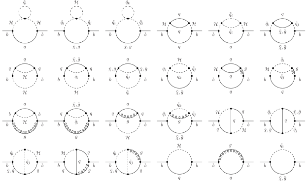
Figure 1: Feynman diagrams contributing to quark self-energies, Here $q$, $\tilde{q}_{i}$, $g$, $\tilde{g}$ denote quark, squark, gluon and gluino fields respectively, ${\cal H}=\{h_{0},H_{0},A_{0},G_{0},H^{+},G^{+}\}$ corresponds to various Higgs fields and $\tilde{\chi}=\{\tilde{\chi}_{0},\tilde{\chi}^{+}\}$ are higgsino states. Two-loop diagrams of the order ${\cal O}(\alpha_{s}^{2})$ are not presented here (see, e.g [7]).

Due to presence of many different mass scales, the problem of exact evaluation of two-loop diagrams is rather complex. Exploiting the fact that

$$m_{b}\ll m_{t},m_{h_{0}},m_{H_{0}},m_{H^{+}},m_{\tilde{q}},m_{{\tilde{\chi}}^{0}},m_{{\tilde{\chi}}^{+}},m_{G_{0}},m_{G^{+}},$$ (8)

where $m_{b}$ and $m_{t}$ are masses of bottom and top quarks, respectively, $m_{h_{0}},m_{H_{0}},m_{H^{+}}$ are masses of the Higgs bosons, $m_{{\tilde{\chi}}^{0}}$ is the neutralino mass, $m_{{\tilde{\chi}}^{+}}$ is the chargino mass, $m_{\tilde{q}}$ are masses of different squarks, $m_{G_{0}},m_{G^{+}}$ are masses of pseudo-goldstone bosons, we use the method of large mass expansion [9] to reduce the evaluation of multi-scale two-loop diagrams to the calculation of two-loop vacuum integrals and products of one-loop on-shell propagator-type diagrams and one-loop bubble integrals. We include only terms up to $\mathcal{O}(m_{b}^{2}/M_{hard}^{2})$, where $M_{hard}$ denotes any mass of the right hand side of (8).

A general Feynman diagram $F_{\Gamma}$ which depends on the large masses $M_{1},M_{2},\ldots,$ small masses $m_{1},m_{2},\ldots$ and small external momenta $p_{1},p_{2},\ldots$ can be expanded as follows [9]:

$$F_{\Gamma}(p_{1},\ldots,M_{1},\ldots,m_{1},\ldots)=\sum_{\gamma}F_{\Gamma/\gamma}(p,m)\mathcal{M}_{\gamma}(p_{\gamma},m)F_{\gamma}(M,m,p_{\gamma}),$$ (9)

where operator $\mathcal{M}_{\gamma}(p_{\gamma},m)$ performs Taylor expansion in small external (with respect to subgraph $\gamma$) momenta and masses. The sum runs over all asymptotically irreducible subgraphs of original graph $\Gamma$.

For calculation of a two-loop propagator diagram that does not have cuts composed of two light lines up to $\mathcal{O}(p^{2}/M^{2})$ one can use naive expansion, when sum in (9) runs over only the trivial subgraph $\gamma=\Gamma$ (see Fig. 2).

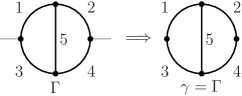
Figure 2: The diagram has no cuts composed of two light lines, therefore the naive expansion can be used.

In case of a diagram that has such a cut a non-trivial subgraph $\gamma_{1}$ has to be taken into account (see Fig. 3).

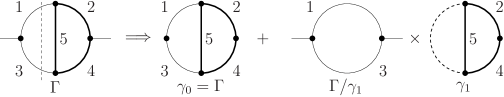
Figure 3: The diagram has one cut composed of two light lines, so non-trivial subgraph $\gamma_{1}$ has to be taken into account.

Two-loop vacuum integrals can be recursively reduced to a master-integral [11] by integration by parts method [12].

Our calculation can be performed in a semi-automatic way. First, FeynArts [13] is used to generate the diagrams. Then the contribution of individual diagrams to the relation (4) is evaluated by means of C++ program TwoLoop, based on GiNaC [14]. TwoLoop [15] performs large mass expansion according to (9), uses recurrence relations of [11] to reduce two-loop vacuum integrals to the master integral, and performs expansion in $\varepsilon$. Results of this calculation were analytically cross-checked using FORM program based on ON-SHELL2 package [16].

After evaluation of two-loop diagrams one should substitute them into (4) and perform renormalization in order to express the correction (7) in terms of running $\overline{\rm DR}$ parameters. Counter-terms were calculated and checked in the same way as in [7], e.g. our renormalization constants for the gauge and Yukawa couplings reproduce well-known $\beta$-functions [17].

3 Numerical results

The analytical result of our calculation is very complicated due to presence of a large number of masses, and no phenomenologically acceptable limit seems to exist. Therefore we present here the numerical analysis of our results.

While a detailed scan over the more-than-hundred-dimensional parameter space of MSSM is clearly not practicable, even a sampling of the three- (four-)dimensional CMSSM parameter space of $m_{0}$, $m_{1/2}$ and $A_{0}$ ($\tan\beta$) is beyond the present capabilities of phenomenological studies, especially when one tries to simulate experimental signatures of supersymmetric particles within a detector. For this reason, one often resorts to specific benchmark scenarios, i.e., one studies only specific parameter points or at best samples the one-dimensional parameter space [18, 19]

Numerical values of running SUSY parameters at the $M_{Z}$ scale have been calculated as a function of CMSSM parameters with the program TwoLoop [15] after interfacing it to a slightly modified version of SOFTSUSY [20] in the framework of mSUGRA supersymmetry breaking scenario. We only consider $\mu>0$ and large values of $\tan\beta$, since small $\tan\beta$ and negative $\mu$ seem to be excluded by experimental data [2].

Fig. 4 shows $m_{1/2}$-dependence of ${\mathcal{O}}(\alpha_{s}^{2})$ [7] and ${\mathcal{O}}(\alpha_{s}y^{2}+y^{4})$ MSSM contributions to (7). For comparison, full one-loop MSSM correction was plotted. Numerical value of the ${\mathcal{O}}(\alpha_{s}^{2})$ contribution is comparable with the full one-loop result, so neglecting other two-loop MSSM corrections leads to a contradiction with the perturbation theory. The ${\mathcal{O}}(\alpha_{s}y^{2}+y^{4})$ contribution is negative in a wide range of the CMSSM parameter space and reduces ${\mathcal{O}}(\alpha_{s}^{2})$ contribution by approximately $30-80\%$. As a consequence ${\mathcal{O}}(\alpha_{s}^{2}+\alpha_{s}y^{2}+y^{4})$ two-loop correction appears to be less than 40% of the one-loop contribution and therefore can be used in phenomenological studies of CMSSM.

Varying $A_{0}$ in a wide range from $-1000\;{\rm GeV}$ to $1000\;{\rm GeV}$ does not change the behaviour of ${\mathcal{O}}(\alpha_{s}^{2}+\alpha_{s}y^{2}+y^{4})$ correction significantly, as one can see from Fig. 4. To make this fact more clear, several curves corresponding to different values of $A_{0}$ were plotted in Fig. 5.

In Fig. 6 we present dependence of different two-loop MSSM contributions on $m_{0}$. For $m_{1/2}\gtrsim 500\;{\rm GeV}$ the change of $m_{0}$ from $400\;{\rm GeV}$ to $1000\;{\rm GeV}$ yields change of ${\mathcal{O}}(\alpha_{s}y^{2}+y^{4})$ correction less than 10%. On the other hand, dependence of ${\mathcal{O}}(\alpha_{s}y^{2}+y^{4})$ correction on $m_{0}$ becomes essential for relatively small $m_{1/2}\;(m_{1/2}\approx 200\;{\rm GeV})$.

It should be noted, that in considered range of CMSSM parameters space ${\mathcal{O}}(\alpha_{s}^{2}+\alpha_{s}y^{2}+y^{4})$ correction is positive.

4 Conclusion

In this paper we presented the results of calculation of the two-loop corrections to the relation between pole and running massess of the $b$-quark, proportional to the Yukawa couplings of heavy quarks ($y_{t},y_{b}$). We provided a numerical analysis of the value of these corrections in different regions of the CMSSM parameter space. Corrections presented here can be used in a renormalization group analysis of the Yukawa coupling unification. It was also found that $m_{b}$ corrections significantly affect low energy phenomenology where the $b$-quark enters [21]. The analysis given in [22] showed that the neutralino relic density is very sensitive to the mass of the $b$-quark for large $\tan\beta$, thus the result considered in this paper may have important implications to the dark matter searches. We are going to study these issues and calculate more ${\mathcal{O}}(\alpha_{s}^{2})$ terms in the large mass expansion of the relation between the top pole and $\overline{\rm DR}$ masses, which requires some improvement of our code.

The authors would like to thank M.Kalmykov, D.Kazakov, A.Onishchenko, V.Velizhanin and O.Veretin for fruitful discussions and multiple comments. Financial support from RFBR grant # 02-02-16889, the grant of Russian Ministry of Industry, Science and Technologies # 2339.2003.2, DFG grant 436 RUS 113/626/0-1 and the Heisenberg-Landau Programme is kindly acknowledged.

Figure 4: Different MSSM contributions to $\Delta m_{b}(M_{Z})/m_{b}(M_{Z})$. Here $m_{0}=1000\;{\rm GeV}$, left column corresponds to $\tan\beta=35$, right column corresponds to $\tan\beta=50$.

Figure 5: $A_{0}$ dependence of ${\mathcal{O}}(\alpha_{s}^{2}+y^{4}+\alpha_{s}y^{2})$ two-loop correction to $\Delta m_{b}(M_{Z})/m_{b}(M_{Z})$. Here $m_{0}=1000\;{\rm GeV}$. Varying $A_{0}$ from $-1000\;{\rm GeV}$ to $1000\;{\rm GeV}$ does not change behaviour of the correction significantly.

Figure 6: Different two-loop MSSM corrections to $\Delta m_{b}(M_{Z})/m_{b}(M_{Z})$ as a function of $m_{0}$. Here $m_{0}=1000\;{\rm GeV},A_{0}=0,\tan\beta=50$. Dependence of ${\mathcal{O}}(\alpha_{s}y^{2}+y^{4})$ correction on $m_{0}$ is essential for $m_{1/2}=200\;{\rm GeV}$. On the other hand, for $m_{1/2}=700\;{\rm GeV}$ the change of $m_{0}$ from $400\;{\rm GeV}$ to $1000\;{\rm GeV}$ yields change of ${\mathcal{O}}(\alpha_{s}y^{2}+y^{4})$ correction less than 10%.

References

- [1] J. R. Ellis, K. A. Olive, Y. Santoso and V. C. Spanos, arXiv:hep-ph/0408118.
- [2] W. de Boer and C. Sander, Phys. Lett. B 585, 276 (2004) [arXiv:hep-ph/0307049].
- [3] H. Baer, C. Balazs, A. Belyaev, T. Krupovnickas and X. Tata, JHEP 0306, 054 (2003) [arXiv:hep-ph/0304303].
- [4] W. de Boer, M. Huber, A. V. Gladyshev and D. I. Kazakov, Eur. Phys. J. C 20, 689 (2001) [arXiv:hep-ph/0102163].
- [5] S. Abel et al. [SUGRA Working Group Collaboration], arXiv:hep-ph/0003154.
- [6] D. M. Pierce, J. A. Bagger, K. T. Matchev and R. j. Zhang, Nucl. Phys. B 491, 3 (1997) [arXiv:hep-ph/9606211].
- [7] A. Bednyakov, A. Onishchenko, V. Velizhanin and O. Veretin, Eur. Phys. J. C 29, 87 (2003) [arXiv:hep-ph/0210258].
- [8] W. Siegel, Phys. Lett. B 84, 193 (1979).
- [9] V. A. Smirnov, “Applied asymptotic expansions in momenta and masses,” http://www.slac.stanford.edu/spires/find/hep/www?irn=4841620
- [10] L. V. Avdeev and M. Y. Kalmykov, Nucl. Phys. B 502, 419 (1997) [arXiv:hep-ph/9701308].
- [11] A. I. Davydychev and J. B. Tausk, Nucl. Phys. B 397, 123 (1993).
- [12] K. G. Chetyrkin and F. V. Tkachov, Nucl. Phys. B 192, 159 (1981).
- [13] T. Hahn and C. Schappacher, Comput. Phys. Commun. 143, 54 (2002) [arXiv:hep-ph/0105349].
- [14] C. Bauer, A. Frink and R. Kreckel, arXiv:cs.sc/0004015.
- [15] A. Sheplyakov, “TwoLoop, C++ library for large mass expansion of 2-loop propagator-type diagrams” (in preparation).
- [16] J. Fleischer and M. Y. Kalmykov, Comput. Phys. Commun. 128, 531 (2000) [arXiv:hep-ph/9907431].
- [17] L. E. Ibanez, C. Lopez and C. Munoz, Nucl. Phys. B 256, 218 (1985).
- [18] S.P. Martin, http://zippy.physics.niu.edu/modellines.html
- [19] S. P. Martin, S. Moretti, J. m. Qian and G. W. Wilson, in Proc. of the APS/DPF/DPB Summer Study on the Future of Particle Physics (Snowmass 2001) ed. N. Graf, eConf C010630, P346 (2001).
- [20] B. C. Allanach, Comput. Phys. Commun. 143, 305 (2002) [arXiv:hep-ph/0104145].
- [21] T. Ibrahim and P. Nath, Phys. Rev. D 68, 015008 (2003) [arXiv:hep-ph/0305201].
- [22] M. E. Gomez, T. Ibrahim, P. Nath and S. Skadhauge, Phys. Rev. D 70, 035014 (2004) [arXiv:hep-ph/0404025].