Equation of state of deconfined matter within dynamical quasiparticle description

Abstract

A simple quasiparticle model, motivated by lowest-order perturbative QCD, is proposed. It is applied to interpret the lattice QCD equation of state. A reasonable reproduction of the lattice data is obtained. In contrast to existing quasiparticle models, the present model is formulated in dynamical rather than thermodynamical terms, and is easily applicable to a system with finite baryon density. In particular, the model simulates the confinement property.
PACS numbers: 12.38.Mh, 12.39.Hg, 24.85.+p

I Introduction

The most fundamental way to compute properties of strongly interacting matter and, in particular, its equation of state (EoS) is provided by lattice QCD calculations latEoS0 . The technique of these calculations rapidly progresses. Recently, lattice data on the EoS at finite baryon chemical potential became available latEoS ; Allton ; Gavai . Interpretation of these data within the straightforward QCD perturbation theory Arnold is hardly possible in view of its extremely poor convergence for any temperature of practical interest. To overcome this poor convergence, resummation schemes were developed. A scheme based on hard-thermal-loop (HTL) effective action Pisarski have been proposed, with alternative formulations in the form of so-called HTL perturbation theory Andersen or based on the $\Phi$-derivable approximation Blaizot . This approach justified a picture of weakly interacting quasiparticles, as determined by the HTL propagators, and resulted in remarkably good agreement with lattice data above $3T_{C}$, with $T_{C}$ being the critical temperature of the phase transition. It is important to emphasize that this quasiparicle picture emerges directly from the QCD dynamics, although treated within the thermal framework. Recently, a new resummation scheme based on dimensionally reduced screened perturbation theory (DRSPT) was proposed Blaizot03 . In certain sense, the efficiency of this DRSPT scheme even surpasses that of the HTL perturbation theory. However, it still gives reliable results only above $2.5T_{C}$.

To extend this perturbative description below $3T_{C}$, various phenomenological quasiparticle models Gorenstein95 ; Greiner ; Levai ; Pesh96 ; Szabo03 ; Rebhan03 ; Weise01 were proposed. These models are formulated in terms of massive quarks and gluons and are constructed in such a way that at high temperatures they match the perturbative results and then extend them down in temperature. It is not clear, if a quasiparicle picture is relevant below $3T_{C}$ at all. Therefore, all these models are purely phenomenological. Nevertheless, interpretation of lattice data within these quasiparticle models turned out to be very successful. With few phenomenological parameters it was possible to reasonably reproduce all lattice thermodynamic quantities. The feature of all above cited quasiparticle models, which still looks slightly irritating, is that they are formulated in terms of thermodynamic quantities (i.e. temperature $T$ and baryon chemical potential $\mu$) rather than dynamical ones, like various densities. From the theoretical point of view, the quasiparticle picture should be formulated in dynamical terms. The thermal equilibrium is only a particular case of this general picture. From the practical point of view, if the quasiparticle is introduced as a dynamical object, it would be possible to use a quasiparticle model for extending the equilibrium lattice description to (at least, slightly) nonequilibrium configurations, relying on reasonable reproduction of equilibrium properties by this model. Such kind of extension is really required for analyzing heavy-ion collisions, where the thermalization is still a debating problem.

In the present paper we propose a simple quasiparticle model formulated in dynamical terms. In construction of this model, we proceed from properties of the perturbative solution to QCD, justifying the quasiparticle picture, rather than from first principles of QCD.

II Dynamical Quasiparticles

Here we will follow the line of Refs. Gorenstein95 ; Pesh96 ; Szabo03 ; Rebhan03 , assuming only massive quasiparticles and avoiding artificial reduction of quark–gluon degrees of freedom as in Weise01 . Let the effective Lagrangian for transverse gluons $\phi_{a}$ and quarks $\psi_{qc}$ of $N_{f}$ flavors be as follows

$${\mathcal{L}} = \frac{1}{2}\sum_{a=1}^{N_{g}}\left((\partial_{\mu}\phi_{a})^{2}-m_{g}^{2}(\eta,{\mbox{\boldmath$\xi$}})\phi_{a}^{2}\right)$$ (1)

$$+ \sum_{c=1}^{N_{c}}\sum_{q=1}^{N_{f}}\bar{\psi}_{qc}[i\gamma_{\mu}\partial^{\mu}-m_{q}(\eta,{\mbox{\boldmath$\xi$}})]\psi_{qc}-B(\eta,{\mbox{\boldmath$\xi$}}),$$ (2)

where $N_{c}=3$ is number of colors, $N_{g}=2(N_{c}^{2}-1)$ is number of transverse gluons, taking into account two transverse polarizations, $m_{g}$ and $m_{q}$ are effective masses of gluons and quarks, respectively, depending on self-consistent fields $\eta$ and ${\mbox{\boldmath$\xi$}}=\{\xi_{1},...,\xi_{N_{f}}\}$. $B(\eta,{\mbox{\boldmath$\xi$}})$ is a potential of mean-field self-interaction. Writing down Lagrangian (1) we have omitted kinetic terms of the $\eta$ and $\xi$ fields, assuming that they are not essential for the problem. Note that these kinetic terms are precisely zero in the spatially homogeneous equilibrium and hence are really negligible for slight deviations from it. This Lagrangian is written proceeding from general features of the perturbative solution to QCD, which claims that quarks and transverse gluons are weakly interacting quasiparticles. Here all interactions between gluons and quarks, as well as their self-interactions, are hidden in their effective masses depending on mean fields, which in their turn are determined in terms of these masses.

Equations of motion for the mean fields are derived in the standard way:

$$-\frac{\partial B}{\partial\eta^{2}} = \frac{1}{2}\frac{\partial m_{g}^{2}}{\partial\eta^{2}}\sum_{a=1}^{N_{g}}\left\langle\phi_{a}^{2}\right\rangle+\frac{1}{2}\sum_{q=1}^{N_{f}}\frac{\partial m_{q}^{2}}{\partial\eta^{2}}\sum_{c=1}^{N_{c}}\frac{\left\langle\bar{\psi}_{qc}\psi_{qc}\right\rangle}{m_{q}},$$ (3)

$$-\frac{\partial B}{\partial\xi_{i}^{2}} = \frac{1}{2}\frac{\partial m_{g}^{2}}{\partial\xi_{i}^{2}}\sum_{a=1}^{N_{g}}\left\langle\phi_{a}^{2}\right\rangle+\frac{1}{2}\sum_{q=1}^{N_{f}}\frac{\partial m_{q}^{2}}{\partial\xi_{i}^{2}}\sum_{c=1}^{N_{c}}\frac{\left\langle\bar{\psi}_{qc}\psi_{qc}\right\rangle}{m_{q}}.$$ (4)

Here

$$\sum_{a=1}^{N_{g}}\left\langle\phi_{a}^{2}\right\rangle = \frac{N_{g}}{2\pi^{2}}\int_{0}^{\infty}\frac{k^{2}\;dk}{(k^{2}+m_{g}^{2})^{1/2}}f_{g}(x,k),$$ (5)

$$\sum_{c=1}^{N_{c}}\frac{\left\langle\bar{\psi}_{qc}\psi_{qc}\right\rangle}{m_{q}} = \frac{N_{c}}{\pi^{2}}\int_{0}^{\infty}\frac{k^{2}\;dk}{(k^{2}+m_{q}^{2})^{1/2}}[f_{q}(x,k)+f_{\bar{q}}(x,k)]$$ (6)

are scalar densities of gluons and quarks divided by mass, respectively, with $f_{g}(x,k)$, $f_{q}(x,k)$ and $f_{\bar{q}}(x,k)$ being distribution functions of gluons, quarks and antiquarks in space–time ($x$) and 4-momenta ($k$). In the particular case of thermal equilibrium we going to consider here, these are

$$f_{g}(k) = \frac{1}{\exp[(k^{2}+m_{g}^{2})^{1/2}/T]-1},$$ (7)

$$f_{q}(k) = \frac{1}{\exp\{[(k^{2}+m_{q}^{2})^{1/2}-\mu_{q}]/T\}+1},$$ (8)

$$f_{\bar{q}}(k) = \frac{1}{\exp\{[(k^{2}+m_{q}^{2})^{1/2}+\mu_{q}]/T\}+1}.$$ (9)

where $T$ is the temperature, and $\mu_{q}$ is the $q$-quark chemical potential. In general, all $\mu_{q}$ may be different. If we consider a system with zero overall strangeness and charm, $\mu_{q}$ relates to the baryon chemical potential as $\mu_{u}=\mu_{d}=\mu/3$ with all other $\mu_{q}=0$.

A solution of Eqs (3) and (4), which are usually referred as gap equations, provides us with an expressions of fields $\eta$ and $\xi_{q}$ in terms of above scalar densities. Without loosing generality, it is convenient to demand that these solutions for the $\eta$ and $\xi$ fields are given by scalar densities of gluons and quarks divided by mass

$$\eta^{2} = \sum_{a=1}^{N_{g}}\left\langle\phi_{a}^{2}\right\rangle,$$ (10)

$$\xi_{q}^{2} = \sum_{c=1}^{N_{c}}\frac{\left\langle\bar{\psi}_{qc}\psi_{qc}\right\rangle}{m_{q}}.$$ (11)

Indeed, had we started from other collective variables $\widetilde{\eta}$ and $\widetilde{\mbox{\boldmath$\xi$}}$, which differ from $\eta$ and $\xi$ defined by Eqs (10) and (11), and the corresponding potential $\widetilde{B}(\widetilde{\eta},\widetilde{\mbox{\boldmath$\xi$}})$, equations of motion (3) and (4) would provide us with solutions $\widetilde{\eta}(\eta,{\mbox{\boldmath$\xi$}})$ and $\widetilde{\mbox{\boldmath$\xi$}}(\eta,{\mbox{\boldmath$\xi$}})$ with $\eta$ and $\xi$ associated with densities (10) and (11). Then we could immediately redefine the potential as $B(\eta,{\mbox{\boldmath$\xi$}})=\widetilde{B}(\widetilde{\eta}(\eta,{\mbox{\boldmath$\xi$}}),\widetilde{\mbox{\boldmath$\xi$}}(\eta,{\mbox{\boldmath$\xi$}}))$ and thus transform to desired variables $\eta$ and $\xi$.

The high-temperature limit, $T\gg T_{C}$, where $T_{C}$ is the temperature of the deconfinement phase transition, puts certain constrains on the functional dependence of the effective masses $m_{g}(\eta,{\mbox{\boldmath$\xi$}})$ and $m_{q}(\eta,{\mbox{\boldmath$\xi$}})$. In this limit, the straightforward calculation of above scalar densities in the leading order results in

$$\eta^{2}(T\gg T_{C}) \simeq \frac{N_{g}}{12}T^{2},$$ (12)

$$\xi_{q}^{2}(\mu_{q},T\gg T_{C}) \simeq N_{c}\left(\frac{1}{6}T^{2}+\frac{1}{2\pi^{2}}\mu_{q}^{2}\right).$$ (13)

Perturbative values of $m_{g}$ and $m_{q}$ are also known Lebel96

$$m_{g}^{2}(\{\mu_{q}\},T\gg T_{C}) = \frac{1}{12}\left((2N_{c}+N_{f}^{\mbox{\scriptsize eff}})T^{2}+\frac{3}{\pi^{2}}\sum_{q=1}^{N_{f}^{\mbox{\scriptsize eff}}}\mu_{q}^{2}\right)g^{2}(\{\mu_{q}\},T\gg T_{C}),$$ (14)

$$m_{q}^{2}(\{\mu_{q}\},T\gg T_{C})-m_{q0}^{2} = \frac{N_{g}}{16N_{c}}\left(T^{2}+\frac{\mu_{q}^{2}}{\pi^{2}}\right)g^{2}(\{\mu_{q}\},T\gg T_{C}),$$ (15)

where $m_{q0}$ is the current mass of the $q$-quark, $N_{f}^{\mbox{\scriptsize eff}}$ is the effective number of quark flavors which can be excited, and $g^{2}$ is the QCD running coupling constant squared, generally depending on $T$ and all $\mu_{q}$. In the particular case of all $\mu_{q}=0$, the latter is also known Yndurain ; Kapusta , in the 2-loop approximation it is

$$g^{2}(\{\mu_{q}=0\},T\gg T_{C})=\frac{16\pi^{2}}{\beta_{0}\ln(2\pi T/\Lambda)^{2}}\left(1-\frac{2\beta_{1}}{\beta_{0}^{2}}\frac{\ln\ln(2\pi T/\Lambda)^{2}}{\ln(2\pi T/\Lambda)^{2}}\right)$$ (16)

with

$$\beta_{0}=\frac{1}{3}(11N_{c}-2N_{f}^{\mbox{\scriptsize eff}}),\quad\beta_{1}=\frac{1}{6}(34N_{c}^{2}-13N_{c}N_{f}^{\mbox{\scriptsize eff}}+3N_{f}^{\mbox{\scriptsize eff}}/N_{c}),$$ (17)

and $\Lambda$ being the QCD scale. The energy scale is taken here equal to $2\pi T$, i.e. the first nonzero Mastubara frequency. In HTL calculations this scale is sometimes varied from $\pi T$ to $4\pi T$ to determine theoretical error bars.

Expressing $T$ and all $\mu_{q}$ in terms of scalar densities $\eta$ and $\xi$ of Eqs. (12) and (13), and substituting them into expressions for asymptotic effective masses (14) and (15), we arrive at the following expressions for the latter

$$m_{g}^{2}(\eta,{\mbox{\boldmath$\xi$}}) = \left(\frac{2N_{c}}{N_{g}}\eta^{2}+\frac{1}{2N_{c}}\sum_{q=1}^{N_{f}}\xi_{q}^{2}\right)g^{2}(\eta^{2},{\mbox{\boldmath$\xi$}}),$$ (18)

$$m_{q}^{2}(\eta,{\mbox{\boldmath$\xi$}})-m_{q0}^{2} = \left(\frac{1}{2N_{c}}\eta^{2}+\frac{N_{g}}{8N_{c}^{2}}\xi_{q}^{2}\right)g^{2}(\eta^{2},{\mbox{\boldmath$\xi$}}).$$ (19)

Here we keep $N_{f}$ instead of $N_{f}^{\mbox{\scriptsize eff}}$, since quark densities $\xi_{q}^{2}$ automatically take care of quark contribution, i.e. $\xi_{q}^{2}\approx 0$, if the $q$-quark is too heavy. These expressions give at the same time the ansatz for the effective masses in terms of scalar densities.

Now our goal is to find an appropriate expression for $g^{2}(\eta,{\mbox{\boldmath$\xi$}})$, which takes the limit (16) at $\mu_{q}=0$ and $T\gg T_{C}$, and then to solve gap equations (3) and (4) with respect to $B(\eta,{\mbox{\boldmath$\xi$}})$. Then the quasiparticle model would be completely defined, and we could do any calculations both in thermodynamics and nonequilibrium. Unfortunately, we failed to solve this problem in general, i.e. we have not found an appropriate potential $B$ which is required for calculation of the thermodynamic quantities, cf. Eqs (32) and (34). However, we have found an elegant solution in the particular case, when number of colors equals number of flavors, i.e. $N_{f}=N_{c}$. In fact, this case is quite general for comparison to lattice data as well as for possible applications in astrophysics and heavy-ion physics.

III Particular Case of $N_{f}=N_{c}$

Let us consider a particular case when $N_{f}=N_{c}$ while the quarks may be different, i.e. their current masses $m_{q0}$ as well as chemical potentials $\mu_{q}$ may differ.

Since $N_{f}=N_{c}$, Eqs. (18) and (19) can be represented as follows

$$m_{g}^{2} = \frac{2}{N_{g}}\sum_{q=1}^{N_{f}}\zeta_{q}^{2}g^{2}(\chi),$$ (20)

$$m_{q}^{2}-m_{q0}^{2} = \frac{1}{2N_{c}}\zeta_{q}^{2}g^{2}(\chi),$$ (21)

where

$$\zeta_{q}^{2} = \eta^{2}+\frac{N_{g}}{4N_{c}}\xi_{q}^{2},$$ (22)

$$\chi^{2} = \left(\sum_{q=1}^{N_{f}}\zeta_{q}^{4}\right)^{1/2}.$$ (23)

Here we just guessed that the $\chi$ dependence of $g^{2}$ is the proper one. This functional dependence is required to define the potential $B$, with which gap equations (3) and (4) give solutions for masses precisely in the form of Eqs (20) and (21). Indeed, gap Eqs. (3) and (4) in terms of new variables $\zeta_{q}^{2}$ read

$$-\frac{\partial B}{\partial\zeta_{i}^{2}} = \frac{1}{2}\frac{\partial m_{g}^{2}}{\partial\zeta_{i}^{2}}\eta^{2}+\frac{1}{2}\sum_{q=1}^{N_{f}}\frac{\partial(m_{q}^{2}-m_{q0}^{2})}{\partial\zeta_{i}^{2}}\xi_{q}^{2}$$ (24)

$$= \frac{1}{N_{g}}\left(g^{2}+\frac{dg^{2}}{d\chi^{2}}\frac{\zeta_{i}^{2}}{\chi^{2}}\sum_{q=1}^{N_{f}}\zeta_{q}^{2}\right)\eta^{2}+\frac{1}{4N_{c}}\sum_{q=1}^{N_{f}}\left(\delta_{qi}g^{2}+\zeta_{q}^{2}\frac{dg^{2}}{d\chi^{2}}\frac{\zeta_{i}^{2}}{\chi^{2}}\right)\xi_{q}^{2}$$ (25)

$$= \frac{1}{N_{g}}g^{2}\left(\eta^{2}+\frac{N_{g}}{4N_{c}}\xi_{i}^{2}\right)+\frac{1}{N_{g}}\frac{dg^{2}}{d\chi^{2}}\frac{\zeta_{i}^{2}}{\chi^{2}}\sum_{q=1}^{N_{f}}\zeta_{q}^{2}\left(\eta^{2}+\frac{N_{g}}{4N_{c}}\xi_{q}^{2}\right)$$ (26)

$$= \frac{1}{N_{g}}\left(g^{2}+\chi^{2}\frac{dg^{2}}{d\chi^{2}}\right)\zeta_{i}^{2}.$$ (27)

where $i=u,d$ or $s$. In fact, this is the main trick advanced by the peculiar case of $N_{f}=N_{c}$. This relation implies that the potential of mean-field self-interaction $B(\eta,{\mbox{\boldmath$\xi$}})$ is in fact a function of a single variable $\chi$, and gap equations (3) and (4) are reduced to the single one

$$\frac{dB}{d\chi}=-\frac{1}{N_{g}}\chi^{2}\frac{d(\chi^{2}g^{2})}{d\chi},$$ (28)

integration of which is straightforward

$$B(\chi) = B_{C}-\frac{1}{N_{g}}\left[\chi^{4}g^{2}(\chi)-\chi_{C}^{4}g^{2}(\chi_{C})\right]+\frac{2}{N_{g}}\int_{\chi_{C}}^{\chi}d\chi_{1}\chi_{1}^{3}g^{2}(\chi_{1})$$ (29)

with $B_{C}$ being an integration constant. In fact, this function $B(\chi)$ has a meaning of the bag constant of the bag model. However, we will refer $B_{C}$ as the “bag parameter”, since it is really constant.

Thus, we succeeded to determine the $B$ potential, which is required for thermodynamically consistent calculation of thermodynamic quantities (32)–(35). We cannot claim that this is the only possible solution for this $B$, because it was obtained as a result of certain guess. However, this solution works quite well in reproducing lattice data, as it is demonstrated in the next section.

A reasonable ansatz for the coupling constant itself is as follows

$$g^{2}(\chi)=\frac{16\pi^{2}}{\beta_{0}\ln[(\chi^{2}+\chi_{0}^{2})/\chi_{C}^{2}]}f(\chi),$$ (30)

where $\chi_{C}^{2}$ and $\chi_{0}^{2}$ are some phenomenological parameters, and an auxiliary function $f(\chi)$, meeting the condition $f(\chi\to\infty)\to 1$, helps us to choose between 1-loop ($f(\chi)\equiv 1$) and 2-loop asymptotics of the coupling constant, cf. Eq. (16). Two reasonable choices of this auxiliary function are discussed below, in sect. IV. This $g^{2}(\chi^{2})$ indeed takes the limit (16) at $\mu_{q}=0$ and $T\gg T_{C}$, provided $\chi_{0}^{2}\ll\chi_{C}^{2}$ and properly defined $\chi_{C}^{2}$ in terms of $\Lambda$. The proper definition in the case, when the temperature is much larger than all current quark masses, $T\gg m_{q0}$, is as follows

$$\chi_{C}^{2}=\frac{N_{g}N_{c}^{1/2}}{8}\left(\frac{\Lambda}{2\pi}\right)^{2}.$$

It is appropriate to mention here that in spite of the declared case $N_{f}=N_{c}$, we are able to consider less number of flavours, $N_{f}^{\mbox{\scriptsize eff}}<3$, cf. Eq. (17), within the same formalism. To exclude a $q$-quark flavor from the treatment at certain temperature $T$, we should take its current mass to be large: $m_{q0}\gg T$, which implies $m_{q}\gg T$, cf. Eq. (21). In this limit the respective density $\xi_{q}^{2}\to 0$ and simply falls out of the corresponding $\zeta_{q}^{2}$, cf. Eq. (22), and hence out of the calculation scheme for lighter particles. Taking into account that the contribution of this heavy quark into thermodynamic quantities (32)–(35) is negligible as compared with that of lighter particles, we see that this heavy quark turns out to be completely switched off from the calculation, as if it does not exist. If we consider $m_{q0}\gg T\gg T_{C}$, the contribution of this heavy quark disappears even from asymptotic formulas (14) and (15). However, the delicate feature of the present solution is that we still should keep the flavor summation in Eq. (20) running though all 3 flavors, in order to obtain the proper gluon contribution into the gluon mass, even in the case of $m_{q0}\gg T\gg T_{C}$. The reason is that for the heavy quark we still have $\zeta_{q}^{2}=\eta^{2}$, i.e. the gluon density which is nonzero. Thus, e.g. for the 2-flavour case, we should keep $N_{f}=3$ whereas take $N_{f}^{\mbox{\scriptsize eff}}=2$ in Eq. (17) required for definition of the coupling constant (30).

To summarize, the procedure of solving the model equations is as follows. First, we define all the free parameters of the model ($\chi_{C}$, $\chi_{0}$, $B_{C}$), including the auxiliary function $f(\chi)$. Given the temperature $T$ and the set of chemical potentials $\mu_{q}$, implicit set of equations (5), (6), (20)–(23) and (30) should be solved. As a result of this solution, we obtain effective quark and gluon masses and the value of $\chi$ variable, which is required for calculation of $B(\chi)$, cf. Eq. 29). Now, when all the quantities are defined, we can calculate the energy density $\varepsilon(T,\mu)$, pressure $P(T,\mu)$, and baryon density $n_{B}(T,\mu)$ as follows

$$\varepsilon(T,\mu) = \frac{N_{g}}{2\pi^{2}}\int_{0}^{\infty}k^{2}\;dk\;(k^{2}+m_{g}^{2})^{1/2}\;f_{g}(k)$$ (32)

$$+\sum_{q=1}^{N_{f}}\frac{N_{c}}{\pi^{2}}\int_{0}^{\infty}k^{2}\;dk\;(k^{2}+m_{q}^{2})^{1/2}\;[f_{q}(k)+f_{\bar{q}}(k)]+B(\chi),$$

$$P(T,\mu) = \frac{N_{g}}{6\pi^{2}}\int_{0}^{\infty}\frac{k^{4}\;dk}{(k^{2}+m_{g}^{2})^{1/2}}f_{g}(k)$$ (34)

$$+\sum_{q=1}^{N_{f}}\frac{N_{c}}{3\pi^{2}}\int_{0}^{\infty}\frac{k^{4}\;dk}{(k^{2}+m_{q}^{2})^{1/2}}[f_{q}(k)+f_{\bar{q}}(k)]-B(\chi),$$

$$n_{B}(T,\mu) = \frac{1}{3}\sum_{q=1}^{N_{f}}\frac{N_{c}}{\pi^{2}}\int_{0}^{\infty}k^{2}\;dk\;[f_{q}(k)-f_{\bar{q}}(k)].$$ (35)

Note that the thermodynamic consistency is automatically fulfilled in this scheme, since we proceed from a proper Lagrangian formulation.

In particular, we would like to mention that the present model simulates the confinement of quarks and gluons. When temperature and/or chemical potentials decrease, the densities, $\eta^{2}$ and $\xi_{q}^{2}$, and together with them the variable $\chi$ drop down. At some value of $\chi$ the argument of $\ln[(\chi^{2}+\chi_{0}^{2})/\chi_{C}^{2}]$ in Eq. (30) becomes very close to 1, and hence $g^{2}\to\infty$. Thus, there are no solutions to the above equations below certain values of temperature and chemical potentials. This can be interpreted as a kind of confinement.

IV Comparison with Lattice Data

Our goal is to fit the above described model to the recent (2+1) flavour lattice data for nonzero chemical potentials latEoS . To be consistent with these lattice data, we accepted current quark masses $m_{u0}=m_{d0}=$ 65 MeV and $m_{s0}=$ 135 MeV, which were used in these lattice calculations. As we have found out, the actual results of our quasiparticle model are quite insensitive to variation of $m_{q0}$ from above lattice values to the “physical” ones $m_{u0}=m_{d0}=$ 7 MeV and $m_{s0}=$ 150 MeV. The model also involves several phenomenological parameters: the “bag parameter” $B_{C}$, cf. (29), the “QCD scale” $\chi_{C}$ and an auxiliary function $f(\chi)$, cf. (30). Another parameter $\chi_{0}^{2}$, as it was expected, should be taken small $\chi_{0}^{2}\ll\chi_{C}^{2}$. In fact, it shifts the lower limit of integration in the expression for $B(\chi)$, cf. Eq. (29), from the singular point of the coupling constant, cf. Eq. (30), and hence regularizes the calculation of $B(\chi)$. Therefore, it is closely related to the “bag parameter” $B_{C}$, which is an integration constant in the same expression. A change of $\chi_{0}^{2}$ implies the corresponding change of $B_{C}$. In all further calculations we take $\chi_{0}^{2}=0.01\chi_{C}^{2}$, and hence the below stated values of $B_{C}$ correspond only to this choice.

An implicit parameter of our model is the critical temperature $T_{C}$, i.e. the temperature at which the deconfinement phase transition occurs at $\mu=$ 0. We could identify this temperature with that of the end point of the solution discussed above. However, this end point is numerically determined not quite reliably because of the singular behavior of the solution near it. Another reason is that the end-point temperature should not necessary coincide with $T_{C}$. The phase transition at $\mu=$ 0 in the case of (2+1) flavours is of the cross-over type, as it was found in lattice calculations. This implies that a strong interplay between quark–gluon and hadronic degrees of freedom occurs near $T_{C}$, which actually determines the $T_{C}$ value itself. As we completely disregard the hadronic degrees of freedom in the model, we cannot count on proper determinations of $T_{C}$ value. Therefore, we vary $T_{C}$ from the determined end-point temperature to slightly below in order to achieve the best fit of the lattice data.

As for the auxiliary function $f(\chi)$, our first choice was

$$f_{\mbox{\scriptsize 1-loop}}(\chi)\equiv 1,$$ (36)

which we refer as “1-loop” choice, because with this $f_{\mbox{\scriptsize 1-loop}}$ the coupling constant takes the 1-loop perturbative limit at $T\to\infty$, cf. Eq. (16). In this case we are left with only two basic parameters, $\chi_{C}$ and $B_{C}$. These are fitted to reproduce the form of the pressure as a function of temperature at zero chemical potential. However, these two parameters does not allow us to reproduce the overall normalization of the lattice pressure. With this respect, it is suitable to recollect that the overall normalization of the lattice data is somewhat uncertain. Indeed, the lattice calculations were done on lattices with $N_{t}=$ 4 temporal extension latEoS . To transform the raw lattice data into physical ones, i.e. to extrapolate to the continuum case of $N_{t}\to\infty$, the raw data are multiplied by “the dominant $T\to\infty$ correction factors between the $N_{t}=$ 4 and continuum case”, $c_{p}=$ 0.518 and $c_{\mu}=$ 0.446, latEoS . These factors are determined as a ratios of the Stefan–Boltzmann pressure at $\mu=$ 0 ($c_{p}$) and the $\mu$-dependent part of the Stefan–Boltzmann pressure ($c_{\mu}$) to the corresponding values on the $N_{t}=$ 4 lattice latEoS . In view of this uncertainty, it is legal to apply an additional overall normalization factor to the same quantities calculated within quasiparticle model . In order to keep the number of fitting parameters as few as possible, we use a single normalization factor instead of two different ones, $c_{p}$ and $c_{\mu}$, in the lattice calculations. For the best fit of the lattice data the overall normalization factor was chosen equal 0.9 and $T_{C}$ was shifted slightly below the end-point temperature, which by itself was determined quite approximately. Note that the fitted $T_{C}=$ 195 MeV is slightly above its lattice value 175 MeV. The set of parameters is summarized in Table. The result of the fit is presented in Fig. 1. In the same figure, also comparison with 2-flavour lattice data latEoS0 is presented. For the present “1-loop” variant, 2-flavour data are perfectly reproduced with the same set of parameters as for (2+1)-flavour case, only the current mass of the strange quark was taken $m_{s0}=$ 100 GeV in order to suppress its contribution. In this case the result for critical temperature is even better: $T_{C}^{\mbox{\scriptsize(2f)}}=$ 175 MeV, which well complies with its lattice value latEoS0 .

Version	$N_{f}^{\mbox{\scriptsize eff}}$∗	$T_{C}$, MeV	$\chi_{C}$, MeV	$B_{C}/\chi_{C}^{4}$∗∗	$f$-factor∗∗∗	overall normalization factor
“1-loop”	2+1	195	141.3	-97.5	1	0.9
“1-loop”	2∗∗∗∗	175	141.3	-97.5	1	0.9
“2-loop”	2+1	195	119.6	-267.5	2.6	1
“2-loop”	2∗∗∗∗	175	119.6	-262.0	2.6	1

^∗ Please, do not confuse it with $N_{f}$, which should be always $N_{f}=3$.
^∗∗ These $B_{C}$ values correspond to the $\chi_{0}^{2}=0.01\chi_{C}^{2}$ choice.
^∗∗∗ This is the effective value of the auxiliary function $f(\chi)$ in the temperature range under investigation, i.e. from $T_{C}$ to $3T_{C}$.
^∗∗∗∗ $m_{s0}=$ 100 GeV in order to suppress the $s$-quark contribution.

Table: Best fits of quasiparticle parameters to the lattice data latEoS0 ; latEoS .

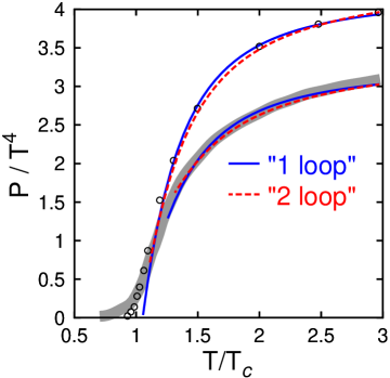
Figure 1: Pressure normalized by $T^{4}$ as a function of $T/T_{c}$ at $\mu=0$. The solid line corresponds to “1-loop” calculation with the overall normalization factor of 0.9. The dashed line represents the “2-loop” calculation. The (2+1)-flavour lattice data latEoS are displayed by open circles, and the 2-flavour lattice data latEoS0 – by grey band.

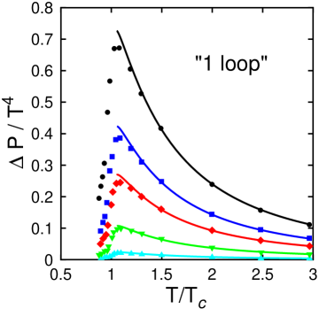
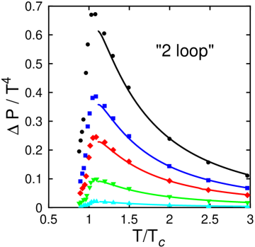
Figure 2: $\Delta P=P(T,\mu)-P(T,\mu=0)$ normalized by $T^{4}$ as a function of $T/T_{c}$ at $\mu=$ 100, 210, 330, 410, 530 MeV (from bottom to top) within the “1-loop” (left panel) and “2-loop” (right panel) calculations. The (2+1)-flavour lattice data are from latEoS .

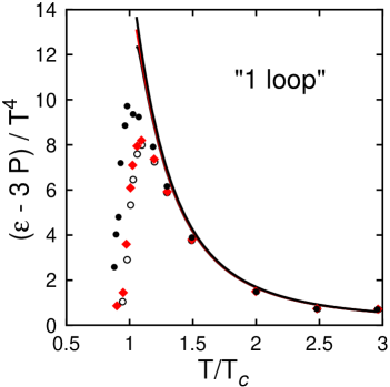
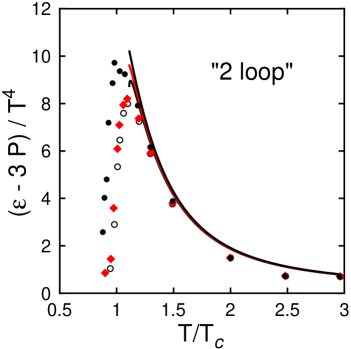
Figure 3: Interaction measure, $\varepsilon-3P$, normalized by $T^{4}$ as a function of $T/T_{c}$ at $\mu=$ 0, 330, 530 MeV (which are hardly distinguishable between each other) within the “1-loop” (left panel) and “2-loop” (right panel) calculations. The (2+1)-flavour lattice data latEoS for different $\mu=$ 0, 330, 530 MeV are displayed by open circles, diamonds and full circles, respectively, similarly to other figures.

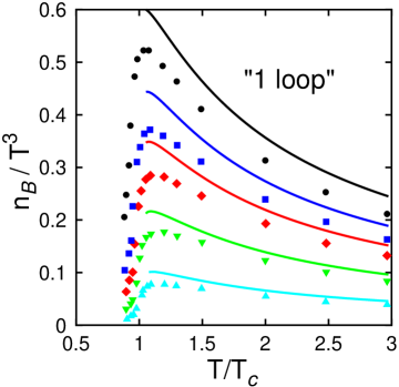
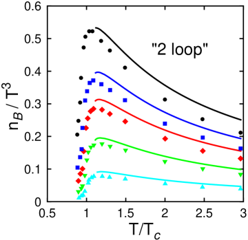
Figure 4: Baryon density normalized by $T^{3}$ as a function of $T/T_{c}$ at $\mu=$ 100, 210, 330, 410, 530 MeV (from bottom to top) within the “1-loop” (left panel) and “2-loop” (right panel) calculations. The (2+1)-flavour lattice data are from latEoS .

Now, when all the parameters are fixed to reproduce the lattice pressure at $\mu=$ 0, all other calculations can be considered as “predictions” of the model. These results are presented in Figs 2–4. The model perfectly reproduces $\mu$-dependent part of the pressure, $\Delta P=P(T,\mu)-P(T,\mu=0)$, Fig. 2, and the “interaction measure”, $\varepsilon-3P$, Fig. 3, at various chemical potentials. In particular, it describes practical $\mu$-independence of the right slope of $\varepsilon-3P$. At the same time, the lattice baryon density, see Fig. 4, turns out to be somewhat overestimated by the model. In fact, this is not surprising, since the thermodynamic consistency of continuum lattice limit is somewhat unbalanced because of application of different normalization coefficients to the raw lattice data: $c_{p}$ and $c_{\mu}$ latEoS mentioned above. Therefore, an exactly thermodynamically consistent model is unable to simultaneously reproduce all the continuum lattice data.

Note that the model fits the lattice quantities only above $T_{C}$. In view of arguments of Ref. Redlich this is not surprising. In Redlich it is argued that below $T_{C}$ these quantities are quantitatively well described by the resonance hadronic gas. From this point of view, we cannot count on proper description below $T_{C}$, since the hadronic degrees of freedom are completely disregarded by the model.

On the other hand, we are able to reproduce the lattice data without varying the overall normalization. However, for this we need nontrivial auxiliary function $f(\chi)$. One of possible choices is

$$f_{\mbox{\scriptsize 2-loop}}(\chi)=1+\arctan\left[\frac{\beta_{1}}{8\pi^{2}\beta_{0}}g^{2}(\chi)\ln\frac{g^{2}(\chi)}{\lambda}\right]$$ (37)

with

$$\lambda=0.001\frac{16\pi^{2}}{\beta_{0}},$$

which we refer as “2-loop” choice, because with this $f_{\mbox{\scriptsize 2-loop}}$ the coupling constant takes the 2-loop perturbative limit at $T\to\infty$, cf. Eq. (16). The additional $g^{2}\ln(0.001)$ term is subleading as compared to $g^{2}(\chi)\ln g^{2}(\chi)$ and thus does not prevent agreement with the 2-loop approximation for coupling constant. In fact, the function $f_{\mbox{\scriptsize 2-loop}}$ is an “exotic” representation of a constant, since in the temperature range under consideration, from $T_{C}$ to $3T_{C}$, it is $f_{\mbox{\scriptsize 2-loop}}(\chi)\simeq$ 2.6 with good accuracy. Precisely this enhancement of the coupling constant is required to fit the actual overall normalization of the lattice data. The reason of using function instead of the constant is only that the function provides us with the proper 2-loop asymptotic limit. In this respect, any function $f$, providing us with additional factor 2.6 in the temperature range from $T_{C}$ to $3T_{C}$ and respecting the proper asymptotic limit of the coupling constant, is as well suitable for this fit. The fitting procedure in this case is completely similar to that for the “1-loop” choice. The obtained sets of parameters for (2+1)- and 2-flavour cases are also summarized in Table. The result of fitting the pressure at $\mu=$ 0 is presented in Fig. 1. The 2-flavour case requires here only slight tune of the $B_{C}$ value as compared to the (2+1)-flavour case. “Predictions” of the “2-loop” version are demonstrated in Figs 2–4. The quality of reproduction of the lattice data here is approximately the same as in the “1-loop” case.

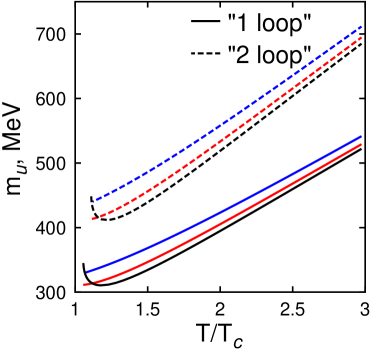
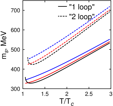
Figure 5: Effective masses of $u$ and $d$ quarks (left panel) and $s$ quark (right panel) as functions of $T/T_{c}$ at $\mu=$ 0, 900, 1500 MeV (from bottom to top). Solid and dashed lines correspond to “1-loop” and “2-loop” calculations, respectively.

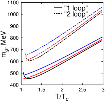
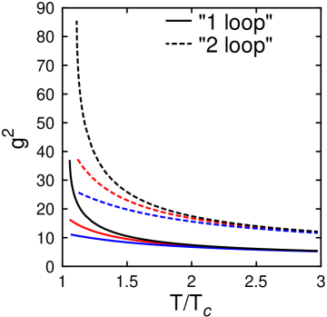
Figure 6: Effective gluon mass (left panel) and coupling constant squared (right panel) as a function of $T/T_{c}$ at $\mu=$ 0, 900, 1500 MeV (from bottom to top in left panel, and from top to bottom in right panel). Solid and dashed lines correspond to “1-loop” and “2-loop” calculations, respectively.

In spite of the similar reproduction of lattice data, the two versions of the model reveal quite different “internal” quantities, see Figs 5 and 6. Their absolute values differ by approximately 30%, while the $T$ and $\mu$ dependences are very similar in the “1-loop” and “2-loop” versions. General trend of these dependences is quite similar to those in the thermodynamic quasiparticle model Szabo03 . Apparently, precisely this trend is essential for reproduction of lattice data within both thermodynamic and present quasiparticle models.

V Summary and Outlook

We have presented a simple quasiparticle model aimed to interpret the lattice QCD data. Similarly to existing quasiparticle approaches Pesh96 ; Szabo03 ; Rebhan03 ; Weise01 , this model is motivated by the lowest-order perturbative QCD. However, contrary to those models , it is formulated in dynamical rather than thermodynamical terms. Presently we have succeeded only for the case $N_{f}\leq N_{c}$, where $N_{f}$ and $N_{c}$ are numbers of quark flavours and colors, respectively. Nevertheless, this is quite a general case for practical applications.

The model has been applied to fit the lattice (2+1)-flavour QCD EoS at finite baryon chemical potentials latEoS . This is the most physical and important from the point of view of practical applications case. However, we fragmentary considered also 2-flavour case . It is demonstrated that a reasonable fit of the quark–gluon sector can be obtained with different sets of phenomenological parameters. The “1-loop” version of the model, cf. Eq. (36), certainly looks more natural, since it does not involve an “exotic” auxiliary function $f$, as it does in the “2-loop” version, cf. Eq. (37). The only problem with the “1-loop” version is that it overestimates all lattice quantities by approximately 10% (and slightly more for the baryonic density). However, since the overall normalization of the lattice data is indeed somewhat uncertain because of the poor extrapolation of these data to the continuum limit, this misfit is quite acceptable.

In spite of the difference in absolute values, “internal” quantities of the model, like effective quark and gluon masses and coupling constant, reveal very similar behaviour as functions of temperature and chemical potential in both “1-loop” and “2-loop” versions. Moreover, this behaviour is also similar to that in thermodynamic quasiparticle models Gorenstein95 ; Greiner ; Levai ; Pesh96 ; Szabo03 ; Rebhan03 ; Weise01 . Apparently, precisely this general trend is essential for reproduction of lattice data within both thermodynamic and present quasiparticle models.

The presented model simulates the confinement of the QCD. In the equilibrium case considered here, the solution to the model equations simply does not exist below certain combination of the temperature and the chemical potential. In particular, this is the reason why we are able to fit the lattice quantities only above $T_{C}$. In Redlich it is argued that below $T_{C}$ these quantities are quantitatively well described by the resonance hadronic gas. From this point of view, we cannot count on proper description below $T_{C}$, since the hadronic degrees of freedom are completely disregarded by the model. From both theoretical and practical points of view, it is desirable to include hadronic degrees of freedom in this model. Then we could count on reproduction of EoS in the whole range of temperatures and chemical potentials. Such a “realistic” EoS would be very useful in hydrodynamic simulations of relativistic heavy-ion collisions.

Acknowledgements

We are grateful to D.N. Voskresensky for fruitful discussions and careful reading of the manuscript. This work was supported in part by the Deutsche Forschungsgemeinschaft (DFG project 436 RUS 113/558/0-2), the Russian Foundation for Basic Research (RFBR grant 03-02-04008) and Russian Minpromnauki (grant NS-1885.2003.2).

References

- (1) F. Karsch, Lect. Notes in Phys. 583, 209 (2002), [hep-lat/0106019]; AIP Conf. Proc. 602, 323 (2001), [hep-lat/0109017].
- (2) Z. Fodor, Nucl. Phys. A715, 319 (2003), [hep-lat/0209101]; F. Csikor, G.I. Egri, Z. Fodor, S.D. Katz, K.K. Szabo, and A.I. Toth, JHEP 405, 46 (2004), [hep-lat/0401016].
- (3) C.R. Allton, S. Ejiri, S.J. Hands, O. Kaczmarek, F. Karsch, E. Laermann, and C. Schmidt, Phys. Rev. D 68, 014507 (2003), [hep-lat/0305007].
- (4) R.V. Gavai and S. Gupta, Phys. Rev. D 68, 034506 (2003), [hep-lat/0303013]
- (5) P. Arnold and C.X. Zhai, Phys. Rev. D 51, 1906 (1995); C.X. Zhai and B. Kastening, Phys. Rev. D 52, 7232 (1995).
- (6) E. Braaten and R.D. Pisarski, Phys. Rev. D 45, R1827 (1992); J. Frenkel and J.C. Taylor, Nucl. Phys. B374, 156 (1992); J.P. Blaizot and E. Iancu, Nucl. Phys. B417, 608 (1994).
- (7) J.O. Andersen, E. Braaten, and M. Strickland, Phys. Rev. Lett. 83, 2139 (1999), [hep-ph/9902327]; Phys. Rev. D 62, 045004 (2000), [hep-ph/0002048]; J.O. Andersen, E. Braaten, E. Petitgirard, and M. Strickland, Phys. Rev. D 66, 085016 (2002), [hep-ph/0205085].
- (8) J.P. Blaizot, E. Iancu, and A. Rebhan, Phys. Rev. Lett. 83, 2906 (1999), [hep-ph/9906340]; Phys. Lett. B470, 181 (1999), [hep-ph/9910309]; Phys. Rev. D 63, 065003 (2001), [hep-ph/0005003].
- (9) K. Kajantie, M. Laine, K. Rummukainen, and Y. Schröder, Phys. Rev. D 67, 105008 (2003), [hep-ph/0211321]; J.P. Blaizot, E. Iancu, and A. Rebhan, Phys. Rev. D 68, 025011 (2003), [hep-ph/0303045]; A. Ipp, A. Rebhan and, A. Vuorinen, Phys. Rev D 69, 077901 (2004), [hep-ph/0311200].
- (10) M.I. Gorenstein and S.N. Yang, Phys. Rev. D 52, 5206 (1995).
- (11) W. Greiner and D.H. Rischke, Phys. Rep. 264, 183 (1996).
- (12) P. Levai and U. Heinz, Phys. Rev. C 57, 1879 (1998), [hep-ph/9710463].
- (13) A. Peshier, B. Kampfer, O.P. Pavlenko, and G. Soff, Phys. Rev. D 54, 2399 (1996); A. Peshier, B. Kampfer, and G. Soff, Phys. Rev. C 61, 045203 (2000), [hep-ph/9911474]; A. Peshier, B. Kampfer, and G. Soff, Phys. Rev. D 66, 094003 (2002) [hep-ph/0206229]; M. Bluhm, B. Kampfer, and G. Soff, hep-ph/0411106.
- (14) K.K. Szabó and A.I. Tóth, JHEP 306, 008 (2003), [hep-ph/0302255].
- (15) A. Rebhan and P. Romatschke, Phys. Rev. D 68, 025022 (2003), [hep-ph/0304294].
- (16) R.A. Schneider and W. Weise, Phys. Rev. C 64, 055201 (2001), [hep-ph/0105242]; T. Renk, R.A. Schneider, and W. Weise, Phys. Rev. C 66, 014902 (2002), [hep-ph/0201048]; M.A. Thaler, R. Schneider, and W. Weise, Phys.Rev. C 69, 035210 (2004), [hep-ph/0310251].
- (17) M. Le Bellac, Thermal Field Theory, Cambridge University Press, Cambridge, 1996.
- (18) J.I. Kapusta, Finite-Temperature Field Theory, Cambridge University Press, Cambridge, 1989.
- (19) F.J. Yndurain, The Theory of Quark and Gluon Interactions, Berlin, Springer-Verlag, 1993.
- (20) F. Karsch, K. Redlich, and A. Tawfik, Eur. Phys. J. C29, 549 (2003), [hep-ph/0303108].