Effective field theories for heavy quarkonium

Abstract

We review recent theoretical developments in heavy quarkonium physics from the point of view of Effective Field Theories of QCD. We discuss Non-Relativistic QCD and concentrate on potential Non-Relativistic QCD. Our main goal will be to derive QCD Schrödinger-like equations that govern heavy quarkonium physics in the weak and strong coupling regime. We also discuss a selected set of applications, which include spectroscopy, inclusive decays and electromagnetic threshold production.

TABLE OF ACRONYMS

For ease of convenience, we list below the acronyms used in the review.

2PI: Two-particle irreducible
2PR: Two-particle reducible
DR: Dimensional Regularization
EFT: Effective Field Theory
IR: Infrared
HQET: Heavy quark effective theory
LO: Leading order
MS: Minimal subtraction
NLO: Next-to-leading order
NNLO: Next-to-next-to-leading order
NNNLO: Next-to-next-to-next-to-leading order
LL: Leading-logarithm order
NLL: Next-to-leading-logarithm order
NNLL: Next-to-next-to-leading-logarithm order
NR: non-relativistic
NRQCD: Non-relativistic Quantum Chromodynamics
NRQED: Non-relativistic Quantum Electrodynamics
pNRQCD: potential Non-relativistic Quantum Chromodynamics
PS: Potential-subtracted
QFT: Quantum Field Theory
QCD: Quantum Chromodynamics
QED: Quantum Electrodynamics
RG: Renormalization group
RS: Renormalon-subtracted
SCET: Soft-collinear effective theory
US: Ultrasoft
UV: Ultraviolet
vNRQCD: velocity Non-relativistic Quantum Chromodynamics

I Introduction

In order to understand human scale processes, a classical NR picture of physics based on Galilean symmetry proves sufficient. Until the beginning of the last century, this picture, supplemented with electromagnetism, was enough in order to understand the majority of processes observed in nature. At the start of the quantum age, it is again a NR equation, the Schrödinger equation, which proved to be the most successful in explaining the atomic and nuclear spectra.

High-energy processes are far away from human scale processes. They are described in present days by relativistic QFTs. Under some circumstances however, high-energy processes develop a NR regime and produce bound states that behave very much like atoms.

The discovery of the $J/\psi$, a heavy resonance with a very narrow width, in Brookhaven and SLAC Aubert et al. (1974); Augustin et al. (1974), which was later on identified with a bound state of a new (heavy) quark, charm, and its antiquark, namely a charmonium ($c{\bar{c}}$) state, opened up the possibility to use a NR picture in the realm of QCD, the fundamental QFT of strong interactions. This possibility was enhanced three years later by the discovery of the $\Upsilon$, an even heavier and narrower resonance, which was again interpreted as a bound state of a new (heavier) quark, bottom, and its antiquark, namely a bottomonium ($b\bar{b}$) state Herb et al. (1977). In fact, the narrow width of these resonances proved to be crucial to establish QCD as the sector of the Standard Model that describes the strong interaction Appelquist and Politzer (1975); De Rujula and Glashow (1975). From that moment on, charmonia and bottomonia have been throughly studied, and still are a subject of intensive theoretical and experimental research (see for instance Skwarnicki (2004); Brambilla et al. (2004)). They can indeed be classified in terms of the quantum numbers of a NR bound state, and the spacing of the radial excitations and of the fine and hyperfine splittings has a pattern similar to the ones in positronium, a well studied QED NR bound state. A related system, the $b{\bar{c}}$ bound state ($B_{c}$) has also been found in nature Abe et al. (1998). The heaviest of the quarks, the top, which has recently been found at Tevatron Abe et al. (1994), has a large decay width (due to weak interactions) and is not expected to form narrow $t$-$\bar{t}$ resonances. However, the production of $t$-$\bar{t}$ near threshold, namely in the NR regime, will be one of the major programs at the Next Linear Collider.

These systems will be denoted by heavy quarkonium. They are characterized by, at least, three widely separated scales: the hard scale (the mass $m$ of the heavy quarks), the soft scale (the relative momentum of the heavy-quark–antiquark $|{\bf p}|\equiv p\sim mv$, $v\ll 1$), and the US scale (the typical kinetic energy $E\sim mv^{2}$ of the heavy quark and antiquark). Moreover, by definition of heavy quark, $m$ is large in comparison with the typical hadronic scale $\Lambda_{\rm QCD}$. Hence, processes that happen at the scale $m$ are expected to be successfully described in perturbation theory, due to the asymptotic freedom of QCD. This explains why the narrow heavy quarkonium widths could be qualitatively understood as a manifestation of asymptotic freedom. However, lower scales, like $|{\bf p}|$ and $E$, which are responsible for the binding, may or may not be accessible to perturbation theory. The appearance of all these scales in the dynamics of heavy quarkonium makes its quantitative study extremely difficult. This is even so in the weak-coupling regime, where the system becomes Coulombic. Nevertheless, by exploiting the hierarchies $m\gg p\gg E$ and $m\gg\Lambda_{\rm QCD}$ the problem can be considerably simplified. This may be done in any particular calculation for a given observable, or, alternatively, using EFTs. In the latter, the hierarchies of scales are exploited at the action level producing universal results independent of particular observables, which is far more advantageous. The basic idea behind EFTs is that to describe observables of a particular (low) energy region, one can integrate out the degrees of freedom of the other regions. This produces an effective action (for the EFT) involving only the degrees of freedom in the region we are interested in. Calculating with the effective (EFT) or with the fundamental (QCD) action gives equivalent physical results as far as that particular region is concerned, but calculations are much simpler with the EFT. In heavy quarkonium, we are interested in physics at the low energy scale $E$. Hence EFTs, which have energy scales larger than $E$ integrated out, can be and have been built. They have led to a major progress in our understanding of heavy quarkonium in recent years. We will devote this review to these new developments. Before that, let us put this progress in a historical perspective.

The discovery of bottomonium and charmonium triggered the use of NR potential models (where the physics of the bound state is described by a Schrödinger equation). The main input in this approach is the potential introduced. At lowest order in the weak-coupling regime ($|{\bf p}|\gg\Lambda_{\rm QCD}$), the potential is Coulombic. Higher-order corrections to the potential in perturbation theory were obtained over the years Gupta and Radford (1981, 1982); Buchmüller et al. (1981); Pantaleone et al. (1986); Titard and Yndurain (1994), even though the computations were difficult due to the several scales involved. It was also not clear how to systematically incorporate US effects (for instance, let us mention the infrared sensitivity found in the static potential Appelquist et al. (1978) or in the one-loop calculations of $P$-wave decays Barbieri et al. (1980)). In any case, the observed bottomonium and charmonium spectra turned out not to be Coulombic and phenomenologically fine-tuned potentials were necessary to reproduce them (Eichten et al. (1978), see Brambilla and Vairo (1999a) for more references). This motivated attempts to derive the heavy-quarkonium potential from QCD without relying on perturbation theory. The idea was to find gauge invariant expressions for the potentials (within an expansion in $1/m$) in terms of the expectation values of Wilson loops. Several methods have been worked out over the years and expressions for the spin-dependent and -independent potentials up to ${\cal O}(1/m^{2})$ were obtained Wilson (1974); Susskind (1977); Brown and Weisberger (1979); Eichten and Feinberg (1981); Peskin (1983); Gromes (1984); Barchielli et al. (1988, 1990); Szczepaniak and Swanson (1997). All the obtained potentials have been investigated on the lattice (see Bali (2001) for a recent review). However, these results had a number of shortcomings. Lucha et al. (1991) pointed out that, if calculated in perturbation theory, the potentials obtained from the Wilson loop approach missed the hard logarithms $\sim\ln m$ present in the potentials directly computed from QCD. More recently, Brambilla et al. (2001b) also pointed out that not only hard logarithms, but some of the potentials, relevant at relative order $\alpha_{\rm s}^{2}$ in the spectrum, were missed as well. Finally, the IR divergences in the perturbative computation of $P$-wave decays seemed impossible to accommodate in that framework. Overall, a more systematic and controlled derivation of the NR dynamics from QCD was required.

Independently of the line above, NRQED, an EFT for NR leptons, was introduced Caswell and Lepage (1986). It turned out to provide the first and decisive link in the chain of developments that we will review here. NRQED is obtained from QED by integrating out the hard scale $m$. It is characterized by an UV cut-off much smaller than the mass $m$ and much larger than any other scale. NRQCD, which also appears in the title of Caswell and Lepage (1986), was born soon afterwards Lepage and Thacker (1988). The Lagrangian of NRQCD can be organized in powers of $1/m$, thus making explicit its NR nature. To each power in $1/m$, a set of operators (which encode the low-energy content of the theory) and matching coefficients (which encode the effects due to degrees of freedom with energy of ${\cal O}(m)$ that have been integrated out from QCD) are associated. Namely, in NRQCD the contributions coming from the hard scale $m$ are factorized. NRQCD had two major virtues that we would like to pont out here: (i) it could be rigorously derived from QCD in a systematic manner (providing an optimized framework for lattice simulations Thacker and Lepage (1991)) and (ii) it solved the problem of the IR divergences of the $P$-wave decays of heavy quarkonium. This solution, however, came to the price of introducing the so-called color-octet matrix elements, which could not be incorporated in the Schrödinger-like formulations available at that time. In spite of this, it was noted in Chen et al. (1995) that if the non-perturbative potentials were calculated starting from NRQCD instead of from QCD, the problem of the missing hard logarithms mentioned above disappeared. This raised again some hope that NR potential models could eventually be regarded as EFTs of QCD. It also made it evident that the potential models available, even those in which the potentials were obtained in terms of Wilson loops, were not controlled derivations from QCD and that first-principles computations of heavy quarkonia should better be done within the framework of NRQCD.

NRQCD itself was, however, not free of shortcomings. The main problem was related to the fact that both soft and US degrees of freedom were entangled. This had effects on (i) the power counting rules, which were not homogeneous (the power counting by Lepage et al. (1992), which assumed that $\Lambda_{\rm QCD}{\ \lower-1.2pt\vbox{\hbox{\hbox to0.0pt{$<$\hss}\lower 6.0pt\vbox{\hbox{$\sim$}}}}\ }mv^{2}$, catches the leading order contribution of the matrix elements but there are also subleading contributions in $v$); and on (ii) the perturbative calculations, which were dependent on two scales and, therefore, still difficult to compute. Another problem was that the first computations in NRQCD were based on cut-off regularization, whereas the calculations in QCD are often done in DR. Attempts to perform the matching between QCD and NRQCD using DR had the drawback that the naive incorporation of the kinetic term in the quark propagator jeopardized the power counting rules.

A solution to the last problem was first proposed by Manohar (1997). There, it was argued that the matching between QCD and NRQCD in the bilinear sector of the theory in DR should be performed just as in HQET (see Neubert (1994) for a review), namely treating the kinetic-energy term as a perturbation. Along the same lines, the matching of QCD to NRQCD in the 4-fermion sector, where the Coulomb pole enhancement starts playing a role, was performed soon after by Pineda and Soto (1998a, c). The key point was that, in order to carry out the matching, it is not so important to know the power counting of each term in the effective theory, but to know that the remaining dynamical scales of the effective theory are much lower than the mass: $m\gg|{\bf p}|,\;E,\;\Lambda_{\rm QCD}$.

Coming back to the main problem, the first works addressing the entanglement of the soft and US scales in NRQCD tried to classify the different momentum regions existing in a purely perturbative version of NRQCD and/or to reformulate NRQCD in such a way that some of these regions were explicitly displayed by introducing new fields in the NRQCD Lagrangian. In particular, we mention Labelle (1998) where a diagrammatic approach to NRQED was used and the subsequent work by Luke and Manohar (1997); Grinstein and Rothstein (1998); Luke and Savage (1998) in NRQCD. All these early attempts turned out to be missing some relevant intermediate degrees of freedom.

The first complete solution came in Pineda and Soto (1998a). The idea was to build an EFT containing only the degrees of freedom relevant for ${\bar{Q}}$–$Q$ systems near threshold, i.e. those with $E\sim mv^{2}$, and as close as possible to a Schrödinger-like formulation (see also Lepage (1997)). All other degrees of freedom were to be integrated out. The EFT, which was called pNRQCD had, roughly, the following structure:

$$\,\left.\begin{array}[]{ll}{\cal L}=\Phi({\bf r})^{\dagger}&\displaystyle{\Bigg{(}i\partial_{0}-{{\bf p}^{2}\over 2m}-V^{(0)}(r)}\\ &\displaystyle{~{}~{}+\hbox{\rm corrections to the potential}}\\ &\displaystyle{~{}~{}+\hbox{interactions with other low-energy degrees of freedom}}\Bigg{)}\Phi({\bf r})\end{array}\right\}{\rm pNRQCD}$$

where $V^{(0)}(r)$ is the static potential ($-C_{F}\alpha_{\rm s}/r$ in the perturbative case) and $\Phi({\bf r})$ is the field associated with the ${\bar{Q}}$–$Q$ state. This EFT turned out to meet all our expectations: it achieved the factorization between US and higher energy modes, had a definite power counting (at least in the perturbative regime), and was very close to a NR Schrödinger-like formulation of the heavy quarkonium dynamics. In the Lagrangian, there appear potentials. These are the matching coefficients of the theory and are calculated by matching with NRQCD amplitudes, either using Feynman diagrams (see Pineda and Soto (1999); Czarnecki et al. (1999b); Beneke et al. (1999); Kniehl et al. (2002b) for specific examples in QCD and QED and sec. IV.5 for further details) or Wilson-loop amplitudes Brambilla et al. (1999b); Brambilla et al. (2000). In the perturbative regime, a confirmation that pNRQCD was able to catch all the relevant dynamical regions came from diagrammatic studies. Beneke and Smirnov (1998) made the most complete classification of (perturbative) momentum regions to date by a diagrammatic study called the threshold expansion. In the language of the threshold expansion, the matching between NRQCD and QCD corresponds to integrating out the hard region and pNRQCD is obtained from NRQCD by integrating out what are called soft quarks and gluons and potential gluons. Finally, we mention two later works, which dealt with reformulating NRQCD within an effective Lagrangian formalism. In Griesshammer (1998) all degrees of freedom of NRQCD were made explicit in the Lagrangian. In Luke et al. (2000) the question on how to obtain RG equations for NR systems was addressed for the first time. The resulting formalism is now known as vNRQCD (for a review on this theory see Hoang (2002)). All these formulations should be equivalent to pNRQCD, once the same degrees of freedom have been integrated out.

This closed the circle, connecting QCD with a properly modified Schrödinger-like formulation in the weak-coupling regime. Compared with the traditional methods, perturbative computations are optimized since only one scale appears in each of the Feynman integrals. The interaction with US gluons is treated in a quantum field theory fashion but yet everything can be encoded in a Schrödinger-like formulation. The applications of these ideas to QED have also been very successful. We refer to sec. IV.7 for references.

The natural question then was: what happens in the strong-coupling regime? The application of EFTs has also led to a well-founded connection with QCD in this regime. The potentials are now understood as matching coefficients to be obtained by comparison with NRQCD. This (along with new computational techniques) has solved the problems mentioned before allowing for the complete computation of the potential at ${\cal O}(1/m^{2})$ Brambilla et al. (2001b); Pineda and Vairo (2001) (as well as identifying new non-analytic terms in the $1/m$ expansion Brambilla et al. (2004)), and the solution of the IR sensitivity of the $P$-wave decays in terms of singlet fields and potentials only Brambilla et al. (2002a). Again, the use of EFTs has allowed to close the circle and connect QCD with a properly modified Schrödinger-like formulation in the strong-coupling regime.

Heavy quarkonium lives nowadays in a new golden age. In the early seventies, its high-energy nature helped to establish asymptotic freedom and QCD as the fundamental theory of the strong interaction. Later on, its NR nature served as a playground for many models of the low-energy dynamics of QCD. Since the nineties, due to the rise of EFTs for heavy quarks, heavy quarkonium observables can be rigorously derived from QCD, low and high energy modes factorized, large logarithms systematically resummed. From a conceptual point of view, the origin and the exact meaning of a QCD Schrödinger-like equation has been clarified. In the weak-coupling regime, this opens up the possibility to have precision determinations of the Standard Model parameters to which heavy quarkonium is sensitive: $\alpha_{\rm s}$ and the heavy quark masses. In the strong-coupling regime, heavy quarkonia are, thanks to their wealth of scales, an ideal laboratory in which to probe the structure of the QCD vacuum.

It is our aim to review here the recent developments in heavy quarkonium physics mentioned above from the point of view of EFTs. Our main goal will be to derive the QCD Schrödinger-like equation that governs heavy quarkonium physics in the weak and strong coupling regime. We will not be exhaustive in most of the derivations but concentrate on the main ideas and general lines of development with spotted examples to illustrate the procedure. Then we will discuss a selected set of applications. The review is not exhaustive. In particular, we will not discuss one of the major phenomenological successes of NRQCD: to provide an explanation of the heavy quarkonium production rate at the Tevatron Braaten et al. (1996); Beneke (1997); Krämer (2001); Bodwin et al. (2003).

Before moving to the main body of the review, we list here our main notational choices Yndurain (1999). The QCD Lagrangian density reads

$${\cal L}=\sum_{i=1}^{N_{f}}\bar{q}_{i}(i\,\raise 0.6458pt\hbox{/}\mkern-13.5muD-m_{i})q_{i}-\frac{1}{4}G^{\mu\nu\,a}G_{\mu\nu}^{a},$$ (2)

where $D_{\mu}=\partial_{\mu}+igA_{\mu}$, $i\,g\,G_{\mu\nu}=[D_{\mu},D_{\nu}]$, $q_{i}$ are the quark fields and $m_{i}$ their current masses. $N_{f}$ is the total number of quark flavors. In the review, we will often indicate with the capital letter, $Q_{i}$, the heavy quark fields and always set to zero the light quark masses. In the EFT, the heavy quark masses will be also indicated by $m_{i}$, but always understood, if not differently specified, as pole masses. The strong-coupling constant, $\alpha_{\rm s}=g^{2}/(4\pi)$, in the presence of $n_{f}$ light quarks runs, at energies below the heavy quark thresholds, as

$$\nu{d\alpha_{\rm s}\over d\nu}=-2\alpha_{\rm s}\left\{\beta_{0}{\alpha_{\rm s}\over 4\pi}+\beta_{1}\left({\alpha_{\rm s}\over 4\pi}\right)^{2}+\cdots\right\},$$ (3)

where

$$\beta_{0}=\frac{11}{3}C_{A}-\frac{4}{3}T_{F}n_{f}\,,\qquad\beta_{1}=\frac{34}{3}C_{A}^{2}-\frac{20}{3}C_{A}T_{F}n_{f}-4\,C_{F}T_{F}n_{f},~{}~{}~{}~{}~{}~{}~{}\dots,$$

and $C_{A}=N_{c}=3$, $C_{F}=(N_{c}^{2}-1)/(2\,N_{c})=4/3$ and $T_{F}=1/2$.

The basic computational techniques for perturbative QCD used through the review can be found in Pascual and Tarrach (1984).

II NRQCD

II.1 Degrees of freedom

NRQCD is designed to describe the dynamics of a heavy quark and a heavy antiquark (not necessarily of the same flavor) at energy scales (in the center of mass frame) much smaller than their masses, which are assumed to be much larger than $\Lambda_{\rm QCD}$, the typical hadronic scale. At these energies, further heavy quark-antiquark pairs cannot be created so it is sufficient, and convenient, to use Pauli spinors for both the heavy quark and the heavy anti-quark degrees of freedom. We shall denote by $\psi(x)$ the Pauli spinor field that annihilates a quark and by $\chi(x)$ the one that creates an antiquark. Both $\psi(x)$ and $\chi(x)$ transform in the fundamental representation of color SU(3). The remaining (light) degrees of freedom are the same as in QCD, except for the UV cut-offs as we shall discuss below. In particular, the gluon fields will appear in covariant derivatives $D_{\mu}$ and field strengths $G_{\mu\nu}$. For instance, we shall see that the leading-order Lagrangian density for the heavy quark and antiquark fields reads

$${\cal L}=\psi^{\dagger}\left(iD_{0}+{1\over 2m}{\bf D}^{2}\right)\psi+\chi^{\dagger}\left(iD_{0}-{1\over 2m}{\bf D}^{2}\right)\chi\,.$$ (4)

In a NR frame, the energy and three-momentum of the heavy particles scale in a different way and hence a different UV cut-off may be introduced for each: $\nu_{s}$ and $\nu_{p}$ respectively. However, NRQCD is usually considered as having a single UV cut-off $\nu_{NR}=\{\nu_{p},\nu_{s}\}$ satisfying $E,p,\Lambda_{\rm QCD}\ll\nu_{NR}\ll m$; $\nu_{p}$ is the UV cut-off of the relative three-momentum of the heavy quark and antiquark; $\nu_{s}$ is the UV cut-off of the energy of the heavy quark and the heavy antiquark, and of the four-momentum of the gluons and light quarks.

From a Wilson RG point of view, NRQCD is obtained from QCD by integrating out energy fluctuations about the heavy quark (heavy antiquark) mass and three-momentum fluctuations up to the scale $\nu_{NR}$ for the heavy quark (heavy antiquark) fields, and four-momentum fluctuations up to the same scale for the fields of the light degrees of freedom. Since $\nu_{NR}\gg\Lambda_{\rm QCD}$, this can be carried out in practice perturbatively in $\alpha_{\rm s}(\nu_{NR})$. Within the threshold expansion framework Beneke and Smirnov (1998), this corresponds to integrating out the hard modes of QCD.

If the quark and antiquark have the same flavor, they can annihilate into hard gluons, which have already been integrated out and are not present in the NRQCD Lagrangian. This implies that, in this case, the QCD Lagrangian must, and will, contain imaginary Wilson coefficients. The non-Hermiticity of the NRQCD Lagrangian, which at first sight may appear rather unpleasant, if not disastrous, turns out to provide an extremely powerful tool for calculating inclusive decay widths to light particles.

II.2 Power counting

From the discussion above, it follows that the NRQCD Lagrangian can be organized as a power series in $1/m_{Q}$ (and $1/m_{\bar{Q}}$). The Wilson (matching) coefficients of each operator depend logarithmically on $m_{Q}$ ($m_{\bar{Q}}$), $\nu_{NR}$ and, as mentioned before, can be calculated in perturbation theory in $\alpha_{\rm s}(\nu_{NR})$. Hence the importance of a given operator for a practical calculation not only depends on its size (power counting), which we will briefly discuss next, but also on the leading power of $\alpha_{\rm s}$ that its matching coefficient has.

Since several scales ($E$, $|{\bf p}|$, $\Lambda_{\rm QCD}$) remain dynamical, it is not possible to assign a size to each operator unambiguously without extra assumptions: no homogeneous power counting exists. As we will see below, the introduction of pNRQCD facilitates this task. The original power counting introduced by Bodwin et al. (1995) assumes $\Lambda_{\rm QCD}\sim E\sim mv^{2}$, and hence $|{\bf p}|\sim mv\gg\Lambda_{\rm QCD}$, $v\sim\alpha_{\rm s}(mv)\ll 1$. We will see that this implies that the bound state is Coulombic (positronium-like). In this case homogeneous power counting rules can be given using pNRQCD in the weak-coupling regime (ch. IV). Nevertheless, it is unlikely that the whole heavy quarkonium spectrum can be described by this power counting and alternatives need to be explored. We only anticipate here that in the strong-coupling regime of pNRQCD the following scaling will be considered: $E\ll|{\bf p}|\sim\Lambda_{\rm QCD}$. The issue of the power counting of NRQCD has also been addressed by Beneke (1997) and Fleming et al. (2001) (see also the discussion in sec. II.6). In both cases, the authors allow for some freedom in the possible size of the NRQCD matrix elements by introducing a parameter $\lambda$ that interpolates between different power countings.

II.3 Lagrangian, currents and symmetries

The allowed operators in the Lagrangian are constrained by the symmetries of QCD. However, due to the particular kinematic region on which we are focusing on, Lorentz invariance is not linearly realized in the heavy quark sector, and it is not straightforward (though certainly possible, as will be discussed below) to implement. One has, in a first stage, to content oneself with implementing the rotational subgroup only. Including $n_{f}$ light quarks, the NRQCD Lagrangian density for a quark of mass $m_{1}$ and an antiquark of mass $m_{2}$ ($m_{1}\;,\;m_{2}\gg\Lambda_{\rm QCD}$) reads at ${\cal O}(1/m^{2})$ , $m=m_{1},m_{2}$ Caswell and Lepage (1986); Bodwin et al. (1995); Manohar (1997); Bauer and Manohar (1998):

$${\cal L}_{\rm NRQCD}={\cal L}_{g}+{\cal L}_{l}+{\cal L}_{\psi}+{\cal L}_{\chi}+{\cal L}_{\psi\chi},$$ (5)

$${\cal L}_{g}=-\frac{1}{4}G^{\mu\nu\,a}G_{\mu\nu}^{a}+{1\over 4}\left({c_{1}^{g\,(1)}\over m_{1}^{2}}+{c_{1}^{g\,(2)}\over m_{2}^{2}}\right)gf_{abc}G_{\mu\nu}^{a}G^{\mu\,b}{}_{\alpha}G^{\nu\alpha\,c},$$ (6)

$${\cal L}_{l}=\sum_{i=1}^{n_{f}}\bar{q}_{i}\,i\,\raise 0.6458pt\hbox{/}\mkern-13.5muD\,q_{i}+{1\over 8}\left({c_{1}^{ll\,(1)}\over m_{1}^{2}}+{c_{1}^{ll\,(2)}\over m_{2}^{2}}\right)\,g^{2}\,\sum_{i,j=1}^{n_{f}}\bar{q_{i}}T^{a}\gamma^{\mu}q_{i}\ \bar{q}_{j}T^{a}\gamma_{\mu}q_{j}$$

$$\qquad\qquad+{1\over 8}\left({c_{2}^{ll\,(1)}\over m_{1}^{2}}+{c_{2}^{ll\,(2)}\over m_{2}^{2}}\right)\,g^{2}\,\sum_{i,j=1}^{n_{f}}\bar{q_{i}}T^{a}\gamma^{\mu}\gamma_{5}q_{i}\ \bar{q}_{j}T^{a}\gamma_{\mu}\gamma_{5}q_{j}$$

$$\qquad\qquad+{1\over 8}\left({c_{3}^{ll\,(1)}\over m_{1}^{2}}+{c_{3}^{ll\,(2)}\over m_{2}^{2}}\right)\,g^{2}\,\sum_{i,j=1}^{n_{f}}\bar{q_{i}}\gamma^{\mu}q_{i}\ \bar{q}_{j}\gamma_{\mu}q_{j}$$

$$\qquad\qquad+{1\over 8}\left({c_{4}^{ll\,(1)}\over m_{1}^{2}}+{c_{4}^{ll\,(2)}\over m_{2}^{2}}\right)\,g^{2}\,\sum_{i,j=1}^{n_{f}}\bar{q_{i}}\gamma^{\mu}\gamma_{5}q_{i}\ \bar{q}_{j}\gamma_{\mu}\gamma_{5}q_{j},$$ (7)

$${\cal L}_{\psi}=\psi^{\dagger}\Biggl{\{}iD_{0}+{c_{k}^{(1)}\over 2m_{1}}{\bf D}^{2}+{c_{4}^{(1)}\over 8m_{1}^{3}}{\bf D}^{4}+{c_{F}^{(1)}\over 2m_{1}}{\mbox{\boldmath$\sigma$}\cdot g{\bf B}}$$

$$\qquad\qquad+{c_{D}^{(1)}\over 8m_{1}^{2}}\left({\bf D}\cdot g{\bf E}-g{\bf E}\cdot{\bf D}\right)+i\,{c_{S}^{(1)}\over 8m_{1}^{2}}{\mbox{\boldmath$\sigma$}\cdot\left({\bf D}\times g{\bf E}-g{\bf E}\times{\bf D}\right)}\Biggr{\}}\psi$$

$$\qquad\qquad+{c_{1}^{hl\,(1)}\over 8m^{2}_{1}}\,g^{2}\,\sum_{i=1}^{n_{f}}\psi^{\dagger}T^{a}\psi\ \bar{q}_{i}\gamma_{0}T^{a}q_{i}+{c_{2}^{hl\,(1)}\over 8m^{2}_{1}}\,g^{2}\,\sum_{i=1}^{n_{f}}\psi^{\dagger}\gamma^{\mu}\gamma_{5}T^{a}\psi\ \bar{q}_{i}\gamma_{\mu}\gamma_{5}T^{a}q_{i}$$

$$\qquad\qquad+{c_{3}^{hl\,(1)}\over 8m^{2}_{1}}\,g^{2}\,\sum_{i=1}^{n_{f}}\psi^{\dagger}\psi\ \bar{q}_{i}\gamma_{0}q_{i}+{c_{4}^{hl\,(1)}\over 8m^{2}_{1}}\,g^{2}\,\sum_{i=1}^{n_{f}}\psi^{\dagger}\gamma^{\mu}\gamma_{5}\psi\ \bar{q}_{i}\gamma_{\mu}\gamma_{5}q_{i},$$ (8)

$${\cal L}_{\chi}=\hbox{c.c. of ${\cal L}_{\psi}(1\leftrightarrow 2)$},$$

$${\cal L}_{\psi\chi}={f_{1}(^{1}S_{0})\over m_{1}m_{2}}O_{1}(^{1}S_{0})+{f_{1}(^{3}S_{1})\over m_{1}m_{2}}O_{1}(^{3}S_{1})+{f_{8}(^{1}S_{0})\over m_{1}m_{2}}O_{8}(^{1}S_{0})+{f_{8}(^{3}S_{1})\over m_{1}m_{2}}O_{8}(^{3}S_{1}),$$ (9)

where

$$O_{1}(^{1}S_{0}) =\psi^{{\dagger}}\chi\,\chi^{{\dagger}}\psi ,\quad O_{1}(^{3}S_{1})=\psi^{{\dagger}}{\mbox{\boldmath$\sigma$}}\chi\,\chi^{{\dagger}}{\mbox{\boldmath$\sigma$}}\psi,$$ (10)

$$O_{8}(^{1}S_{0}) =\psi^{{\dagger}}{\rm T}^{a}\chi\,\chi^{{\dagger}}{\rm T}^{a}\psi ,\quad O_{8}(^{3}S_{1})=\psi^{{\dagger}}{\rm T}^{a}{\mbox{\boldmath$\sigma$}}\chi\,\chi^{{\dagger}}{\rm T}^{a}{\mbox{\boldmath$\sigma$}}\psi.$$ (11)

The matching coefficients are symmetric under the exchange $m_{1}\leftrightarrow m_{2}$, $\sigma$ are the Pauli matrices, $iD^{0}=i\partial^{0}-gA^{0}$, $i{\bf D}=i\mbox{\boldmath$\nabla$}+g{\bf A}$, ${\bf E}^{i}=G^{i0}$, ${\bf B}^{i}=-\epsilon_{ijk}G^{jk}/2$, $\epsilon_{ijk}$ being the usual three-dimensional antisymmetric tensor ($({\bf a}\times{\bf b})^{i}\equiv\epsilon_{ijk}{\bf a}^{j}{\bf b}^{k}$) with $\epsilon_{123}=1$, and c.c. stands for charge conjugate ($\psi^{c}=-i\sigma^{2}\chi^{\ast}$, $\chi^{c}=i\sigma^{2}\psi^{\ast}$ and $A_{\mu}^{c}=-A_{\mu}^{T}$).

The NRQCD Lagrangian is defined up to field redefinitions. In the expression adopted here, we have made use of this freedom. Powers larger than one of $iD_{0}$ applied to the quark fields have been eliminated. We have also redefined the gluon fields in such a way that the coefficient in front of $-G^{\mu\nu\,a}G_{\mu\nu}^{a}/4$ in ${\cal L}_{g}$ is one. This turns out to be equivalent to redefining the coupling constant in such a way that it runs with $N_{f}-2=n_{f}$ flavors (for $m_{1}\neq m_{2}$, $N_{f}-1=n_{f}$ for $m_{1}=m_{2}$), where $N_{f}$ are the flavors in QCD Pineda and Soto (1998c) (see also Griesshammer (2000) for a calculation of the $\beta$ function in NRQCD). A possible term $D^{\mu}\,G_{\mu\alpha}^{a}\,D_{\nu}\,G^{\nu\alpha\,a}$ has been eliminated through the identity Manohar (1997):

$$\int d^{4}x\,\left(2\,D^{\mu}\,G_{\mu\alpha}^{a}\,D_{\nu}\,G^{\nu\alpha\,a}+2\ g\,f_{abc}\,G_{\mu\nu}^{a}G^{\mu\,b}{}_{\alpha}G^{\nu\alpha\,c}+G_{\mu\nu}^{a}\,D^{2}\,G^{\mu\nu\,a}\right)=0.$$ (12)

Finally, a possible term like $c\,G_{\mu\nu}^{a}D^{2}G^{\mu\nu\,a}$ has been eliminated through the field redefinition $A_{\mu}\to A_{\mu}+2\,c\,[D^{\alpha},G_{\alpha\mu}]$ Pineda and Vairo (2001).

The Wilson coefficients appearing in the NRQCD Lagrangian will be discussed in sec. II.4. The ${\cal O}(1/m^{3})$ Lagrangian (without the light-fermion sector) can be found in Manohar (1997). The Feynman rules associated to the first two lines of Eq. (8) can be found in Bodwin and Chen (1999).

NR currents should also be considered, since they appear in inclusive (electromagnetic) decays, NR sum rules or $t$-$\bar{t}$ production near threshold. Similarly to the Lagrangian, they can be written as an expansion in $1/m$ times some hard matching coefficients times some NR (local) operators. For instance, the electromagnetic vector and axial-vector currents read (see Hoang and Teubner (1999))

$$j_{k}^{v}(x) = b^{v}_{1,\rm NR}\,\Big{(}{\psi}^{\dagger}\sigma_{k}\chi\Big{)}(x)-\frac{b^{v}_{2,\rm NR}}{6m^{2}}\,\Big{(}{\psi}^{\dagger}\sigma_{k}(\mbox{$-\frac{i}{2}$}\stackrel{{\scriptstyle\leftrightarrow}}{{\mbox{\boldmath$D$}}})^{2}\chi\Big{)}(x)+\ldots\,,$$ (13)

$$j_{k}^{a}(x) = \frac{b^{a}_{1,\rm NR}}{m}\,\Big{(}{\psi}^{\dagger}(\mbox{$-\frac{i}{2}$}\stackrel{{\scriptstyle\leftrightarrow}}{{\mbox{\boldmath$D$}}}\!\!\times{\mbox{\boldmath$\sigma$}})_{k}\,\chi\Big{)}(x)+\ldots\,,$$ (14)

where $\psi^{\dagger}\stackrel{{\scriptstyle\leftrightarrow}}{{\mbox{\boldmath$D$}}}\chi\equiv\psi^{\dagger}({\bf D}\chi)-({\bf D}\psi)^{\dagger}\chi$ and the dots stand for corrections, which do not contribute at NNLO order for $S$-waves. In practice, most of the physical information can be extracted from the imaginary parts of the 4-fermion operators, which are discussed in sec. II.6.2. In particular, the matching coefficients $b^{v}_{1,\rm NR}$ and $b^{v}_{2,\rm NR}$ can be traded for the matching coefficients Im $f_{\rm EM}({}^{3}S_{1})$ and Im $g_{\rm EM}({}^{3}S_{1})$ respectively.

II.3.1 Poincaré/reparametrization invariance

The QCD Lagrangian is invariant under Lorentz boosts. However, the NR expansion has destroyed the manifest invariance of the EFT under Lorentz boosts. Since the EFT is equivalent to QCD at any order of the strong-coupling and NR expansion, the invariance under Lorentz boosts is not lost, but must be somehow incorporated in the EFT. Indeed, it imposes specific constraints on the form of the EFT itself.

Constraints imposed by the relativistic invariance have been first worked out for HQET, which coincides with NRQCD in the bilinear sector of the heavy-quark fields Luke and Manohar (1992); Manohar (1997). In HQET the realization of the relativistic invariance is called reparametrization invariance. It imposes constraints on the Wilson coefficients of the EFT. For instance:

$$c_{k}=c_{4}=1,\qquad 2\,c_{F}-c_{S}-1=0,\qquad$$ (15)

where we have dropped the explicit indication of the flavor index.

An alternative derivation consists of imposing the Poincaré algebra on the generators $H$, ${\bf P}$, ${\bf J}$ and ${\bf K}$ of time translations, space translations, rotations, and Lorentz-boosts transformations of NRQCD Brambilla et al. (2003b). The idea originates from Dirac (1949), and has been used to constrain the form of the relativistic corrections to phenomenological potentials in Foldy (1961); Krajcik and Foldy (1974); Sebastian and Yun (1979). It was applied to NR EFTs in Brambilla et al. (2003b); Vairo (2004a). In a field theory, the Poincaré algebra has to be understood among fields quantized in accordance with the canonical equal-time commutation relations. The translation and rotation generators ${\bf P}$ and ${\bf J}$ may be derived from the NRQCD Lagrangian or by matching to the QCD generators. They are exact, because translational and rotational invariance have not been explicitly broken in going to the EFT. The Lorentz-boost generators may be obtained by matching order by order in $1/m$ to the Lorentz-boost generators of QCD. They depend on some specific matching coefficients independent of those in the Lagrangian. The NRQCD Poincaré generators satisfy the Poincaré algebra if Eq. (15) is satisfied for each flavor up to ${\cal O}(1/m)$ and ${\cal O}(\mbox{\boldmath$\nabla$}^{2}\,\mbox{\boldmath$\nabla$}/m^{2})$ (plus some other constraints on the matching coefficients appearing in ${\bf K}$)Brambilla et al. (2003b). Therefore, at the considered order, we get the same result as from reparametrization invariance. The calculation of constraints specific to NRQCD, i.e. involving 4-fermion operators, has not been done in either approach yet. This would correspond to going to higher orders in $1/m$.

In general, we will constrain the matching coefficients of the kinetic energy in accordance with Eq. (15). Occasionally, however, we will keep them explicit for tracking purposes.

II.4 Matching

The calculation of the Wilson coefficients of NRQCD is done through a procedure called matching. In a matching calculation suitable renormalized QCD and renormalized NRQCD Green’s functions (or matrix elements) are imposed to be equal for scales below $\nu_{NR}$ at the desired order of $\alpha_{\rm s}$ and $1/m$. In particular, the expansion of Green’s functions in external energies $E$ and three-momenta $p$ must be equal. This fixes the matching coefficients, which will depend on the renormalization schemes used in QCD and in NRQCD. It extraordinarily simplifies calculations if these expansions are done before the loop integrals are performed. However, doing so may introduce IR divergences and for the equality between QCD and NRQCD Green functions to remain valid the same IR regulator must be used in both theories. It is very convenient to use DR as an IR regulator as well as an UV one. This is so because all loop integrals in the NRQCD calculations will be scaleless and can be set to zero, as we will argue below. Let us advance what will happen. Schematically Manohar (1997), one has

$$A_{eff}\left({1\over\epsilon_{UV}}-{1\over\epsilon_{IR}}\right)$$ (16)

in the EFT, which is zero if $\epsilon_{UV}=\epsilon_{IR}$ in DR. Therefore, we only have to calculate loop integrals in QCD that depend on a single scale ($m$). Typically we get

$$A{1\over\epsilon_{UV}}+B{1\over\epsilon_{IR}}+\left(A+B\right)\ln{\nu\over m}+D\,.$$ (17)

Since the full and the effective theory share the same IR behavior $B=-A_{eff}$. Moreover the UV divergences are absorbed in the coefficients of the full and effective theory. In this way the difference between the full and the effective theory reads

$$\left(A+B\right)\ln{\nu\over m}+D\,,$$ (18)

which provides the one-loop contribution to the matching coefficients for the effective theory. It is implicitly in this procedure that the same renormalization scheme is used for both UV and IR divergences in NRQCD. In the QCD calculation both the UV and IR divergences can also be renormalized in the same way, for instance using the $\overline{\rm MS}$ scheme, which is the standard one for QCD calculations. This fixes the UV renormalization scheme in NRQCD in which the Wilson coefficients have been calculated. This means that for these Wilson coefficients to be consistently used in a NRQCD calculation, this calculation must be carried out in the same scheme, for instance in DR and in the $\overline{\rm MS}$ scheme.

The matching calculation can be carried out in any gauge, since both the QCD and NRQCD Lagrangians are manifestly gauge invariant. However, since most of the times one is matching gauge-dependent Green functions, the same gauge must be chosen in QCD and NRQCD. Using different gauges or, in general, different ways to carry out the matching procedure, may lead to apparently different results for the matching coefficients (within the same regularization and renormalization scheme). These results must be related by local field redefinitions, or, in other words, if both matching calculations had agreed to use the same minimal basis of operators beforehand, the results would have coincided. If the matching is carried out as described above, it is more convenient to choose a covariant gauge (i.e. Feynman gauge), since only QCD calculations, which are manifestly covariant, are to be carried out.

In the procedure described above, one may be worried about the fact that the NR propagator $1/(p^{0}-{\bf p}^{2}/m)$ contains the scale $m$, which spoils the usual argument (used in HQET for instance) that loop integrals in the EFT contain no scales once one has expanded in the external energies and three-momenta. Let us argue in the following paragraphs that the procedure is indeed correct.

Consider first the single quark (antiquark) sector. In any diagram in NRQCD, one can always choose the momenta flowing along the heavy quark (antiquark) line in the same direction. Then all heavy quark propagators will have poles in either the lower or the upper half of the complex plane only. Then, if all integrals over the energies flowing through the heavy quark propagators are carried out by closing the contour around the opposite half-complex plane, these energies will be substituted by linear dependencies in the three-momenta in the NR quark (antiquark) propagators. These linear dependencies dominate over quadratic dependencies of the kinetic terms both in the IR and in the UV. The latter is so because $\nu_{NR}$ is always smaller than $m$. Hence the kinetic term can be expanded and the integrals become dimensionless. In fact, in DR the kinetic term not only can but must be expanded, since this is the only way to implement that three-momenta must remain smaller than $\nu_{NR}$.

Consider next the quark-antiquark sector. Any fixed-order loop calculation may contain heavy quark-antiquark irreducible diagrams (meaning diagrams which cannot be disconnected by cutting an internal quark line and an internal antiquark line) and heavy quark-antiquark reducible ones.

Consider first a quark-antiquark irreducible diagram. The fact that at any point of an internal quark propagator there is always at least one gluon propagator (or two light quark propagators) in addition to an antiquark propagator allows to choose all momenta flowing both along the quark and along the antiquark propagator in the same direction. Hence the poles of both the quark and antiquark propagators are in the same complex half-plane, and therefore the argument put forward for the single-quark sector also holds here.

Consider finally a quark-antiquark reducible diagram. It can always be written as a series of 2PI diagrams linked by a quark and by an antiquark propagator. Let us choose the center of mass momentum to be zero and focus on one such 2PI block. If $p$ ($p^{\prime}$) is the momentum flowing along the incoming (outgoing) quark line, then $-p$ ($-p^{\prime}$) is necessarily the momentum flowing along the incoming (outgoing) antiquark line. $p^{0}$ (${p^{0}}^{\prime}$) has two relevant scalings, namely $p^{0}\sim|{\bf p}|$ and $p^{0}\sim{\bf p}^{2}/2m$. If the scaling $p^{0}\sim|{\bf p}|$ occurs, then kinetic terms $\sim{\bf p}^{2}/2m$ can be neglected in the 2PI diagram and no further scale $m$ will be introduced. If the scaling $p^{0}\sim{\bf p}^{2}/2m$ occurs, then $k^{0}$ can be neglected in the gluon propagators and the only dependence in $p^{0}$ can be reduced to either the quark or antiquark propagator. Furthermore, the internal energies in the 2PI diagram eventually take the value of the three-momenta $|{\bf p}|$ and hence $p^{0}$ and ${\bf p}^{2}/2m$ can be expanded. Hence in either case, no extra scales $m$ are introduced in the 2PI diagrams and they can be set to zero. Consider now the link between two 2PI diagrams. If $p^{0}\sim|{\bf p}|$, the kinetic term can be expanded and no further scale $m$ is introduced. If $p^{0}\sim{\bf p}^{2}/2m$, no further dependence on $p^{0}$ in the 2PI diagrams exists, and hence the integral over $p^{0}$ can be trivially done inducing a $m/{\bf p}^{2}$ propagator so that the $m$ dependence factorizes trivially. In summary, 2PR diagrams also become scaleless and can be set to zero.

One might be worried about the appearance of pinch singularities when the kinetic terms are expanded in the links. Let us argue that they are of no concern. Recall first that pinch singularities blow up only after the limit $\eta\rightarrow 0$ is taken, where $i\eta$ defines the causal propagator. We prescribe to take this limit at the end of the calculation. If no other dependence on $p^{0}$ existed, we could carry out all integrals except the one over $p^{0}$. Since they have no scale, as argued before, and they contain no pinch singularities, they can safely be set to zero, and hence the net result is zero. If there are further dependencies on $p^{0}$, by fraction decomposition one can always isolate the pinch singularity in a term $1/(p^{0}+i\eta)(-p^{0}+i\eta)$ with no further dependencies on $p^{0}$ (plus other terms with no pinch singularity) and proceed as above.

Let us finally note that this matching procedure corresponds to taking the purely hard contribution in the threshold expansion for the NRQCD matching coefficients.

In order to address the matching calculation, we also need the relation between the QCD and NRQCD quark (antiquark) fields:

$$Q_{1}(x)\rightarrow Z_{1}^{1\over 2}{1+\gamma_{0}\over 2}e^{-im_{1}t}\psi(x)\quad,\quad Q_{2}(x)\rightarrow Z_{2}^{1\over 2}{1-\gamma_{0}\over 2}e^{im_{2}t}\chi(x)$$ (19)

At one loop, one obtains for the wavefunction renormalization constants

$$Z_{i}=1+C_{F}{\alpha\over\pi}\left({3\over 4}\ln{m_{i}^{2}\over\nu^{2}}-1\right)+{\cal O}\left(\left({\alpha\over\pi}\right)^{2}\right)\quad,\quad i=1,2\,.$$ (20)

Notice also that the states are differently normalized in relativistic ($\left<{\bf p}|{\bf p}^{\prime}\right>=(2\pi)^{3}2\sqrt{{\bf p}^{2}+m^{2}}\delta^{3}({\bf p}-{\bf p}^{\prime})$) or NR ($\left<{\bf p}|{\bf p}^{\prime}\right>=(2\pi)^{3}\delta^{3}({\bf p}-{\bf p}^{\prime})$) theories. Hence, in order to compare the S-matrix elements between the two theories, a factor $(2\sqrt{{\bf p}^{2}+m^{2}})^{1/2}$ has to be introduced for each external fermion.

For the single quark (antiquark) sector as well as for the purely gluonic sector, the matching coefficients have been obtained at one loop up to ${\cal O}(1/m^{2})$ in the background Feynman gauge by Manohar (1997). They read (similarly for $1\rightarrow 2$)

$$c_{F}^{(1)} = 1+{\alpha_{\rm s}\over 2\pi}\left[C_{F}+\left(1-\ln{m_{1}\over\nu}\right)C_{A}\right]\,,$$

$$c_{D}^{(1)} = 1+{\alpha_{\rm s}\over\pi}\left[\left({8\over 3}\ln{m_{1}\over\nu}\right)C_{F}+\left({1\over 2}+{2\over 3}\ln{{m_{1}}\over\nu}\right)C_{A}\right]-{4\over 15}{\alpha_{\rm s}\over\pi}T_{F}\left({m_{1}^{2}+m_{2}^{2}\over m_{2}^{2}}\right)\,,$$

$$c_{S}^{(1)} = 1+{\alpha_{\rm s}\over\pi}\left[C_{F}+\left(1-\ln{m_{1}\over\nu}\right)C_{A}\right]\,,$$

$$c_{1}^{g\,(1)} = {\alpha_{\rm s}\over 360\pi}T_{F}\,,$$ (21)

($\nu=\nu_{NR}$). The complete ${\cal O}(\alpha_{\rm s}^{2})$ correction to $c_{F}$ is also known Czarnecki and Grozin (1997).

For the quark-antiquark sector, they have been obtained at one loop up to ${\cal O}(1/m^{2})$ in Pineda and Soto (1998c). For the non-annihilation diagrams, which are displayed in Fig. 1,

Figure 1: Relevant one-loop diagrams for the matching of the 4-fermion operators at order ${\cal O}(1/m^{2})$ for the case of unequal masses. The incoming and outgoing particles are on-shell and exactly at rest.

it is convenient to use the following basis

$${\cal L}_{\psi\chi} = {d_{ss}\over m_{1}m_{2}}\psi_{1}^{{\dagger}}\psi_{1}\chi_{2}^{{\dagger}}\chi_{2}+{d_{sv}\over m_{1}m_{2}}\psi_{1}^{{\dagger}}{\mbox{\boldmath$\sigma$}}\psi_{1}\chi_{2}^{{\dagger}}{\mbox{\boldmath$\sigma$}}\chi_{2}$$ (22)

$$+{d_{vs}\over m_{1}m_{2}}\psi_{1}^{{\dagger}}{\rm T}^{a}\psi_{1}\chi_{2}^{{\dagger}}{\rm T}^{a}\chi_{2}+{d_{vv}\over m_{1}m_{2}}\psi_{1}^{{\dagger}}{\rm T}^{a}{\mbox{\boldmath$\sigma$}}\psi_{1}\chi_{2}^{{\dagger}}{\rm T}^{a}{\mbox{\boldmath$\sigma$}}\chi_{2}\,,$$

which is equivalent to the one in Eq. (9). The relation between them can be found (in four dimensions) in Pineda and Soto (1998c). In this basis, for the case of the quark and the antiquark having arbitrary flavor, the matching coefficients at one loop read in Feynman gauge

$$d_{ss} = -C_{F}\left({C_{A}\over 2}-C_{F}\right){\alpha_{\rm s}^{2}\over m_{1}^{2}-m^{2}_{2}}\left\{m_{1}^{2}\left(\ln{m^{2}_{2}\over\nu^{2}}+{1\over 3}\right)-m^{2}_{2}\left(\ln{m^{2}_{1}\over\nu^{2}}+{1\over 3}\right)\right\}\,,$$ (23)

$$d_{sv} = C_{F}\left({C_{A}\over 2}-C_{F}\right){\alpha_{\rm s}^{2}\over m_{1}^{2}-m^{2}_{2}}m_{1}m_{2}\ln{m^{2}_{1}\over m^{2}_{2}}\,,$$ (24)

$$d_{vs} = -{2C_{F}\alpha_{\rm s}^{2}\over m_{1}^{2}-m^{2}_{2}}\left\{m_{1}^{2}\left(\ln{m^{2}_{2}\over\nu^{2}}+{1\over 3}\right)-m^{2}_{2}\left(\ln{m^{2}_{1}\over\nu^{2}}+{1\over 3}\right)\right\}$$

$$+{C_{A}\alpha_{\rm s}^{2}\over 4(m_{1}^{2}-m^{2}_{2})}\Biggl{[}3\left\{m_{1}^{2}\left(\ln{m^{2}_{2}\over\nu^{2}}+{1\over 3}\right)-m^{2}_{2}\left(\ln{m^{2}_{1}\over\nu^{2}}+{1\over 3}\right)\right\}$$

$$\quad\quad\quad\quad+{1\over m_{1}m_{2}}\left\{m_{1}^{4}\left(\ln{m^{2}_{2}\over\nu^{2}}+{10\over 3}\right)-m^{4}_{2}\left(\ln{m^{2}_{1}\over\nu^{2}}+{10\over 3}\right)\right\}\Biggr{]}\,,$$

$$d_{vv} = {2C_{F}\alpha_{\rm s}^{2}\over m_{1}^{2}-m^{2}_{2}}m_{1}m_{2}\ln{m^{2}_{1}\over m^{2}_{2}}$$

$$+{C_{A}\alpha_{\rm s}^{2}\over 4(m_{1}^{2}-m^{2}_{2})}\Biggl{[}\left\{m_{1}^{2}\left(\ln{m^{2}_{2}\over\nu^{2}}+3\right)-m^{2}_{2}\left(\ln{m^{2}_{1}\over\nu^{2}}+3\right)\right\}-3m_{1}m_{2}\ln{m^{2}_{1}\over m^{2}_{2}}\Biggr{]}\,.$$

($\nu=\nu_{NR}$). The $\nu$-independent pieces of $d_{vv}$ depend on the prescription for reducing the $D$-dimensional Dirac matrices to Pauli matrices. Note that we have used the prescription for the dimensionally regulated spin matrices of Pineda and Soto (1998c), which differs from the more standard ’t Hooft-Veltman scheme.

The contribution of the diagrams in Fig. 1 to the case of equal flavor is obtained by taking the limit $m_{1}\rightarrow m_{2}=m$. Explicit formulas for this case can be found in Pineda and Soto (1998c). In this case, however, annihilation processes are allowed and they should be taken into account. The relevant annihilation diagrams up to one loop are displayed in Fig. 2.

Figure 2: Relevant diagrams to the matching for the 4-fermion operators at order ${\cal O}(1/m^{2})$ and one loop that only appear for the equal mass case. The incoming and outgoing particles are on-shell and exactly at rest.

One obtains:

$$f_{1}({}^{1}S_{0}) = \alpha_{\rm s}^{2}C_{F}\left({C_{A}\over 2}-C_{F}\right)\left(2-2\ln 2+i\pi\right)\,,$$ (27)

$$f_{1}({}^{3}S_{1}) = 0\,,$$ (28)

$$f_{8}({}^{1}S_{0}) = {\alpha_{\rm s}^{2}\over 2}\left(-{3\over 2}C_{A}+4\,C_{F}\right)\left(2-2\ln 2+i\pi\right)\,,$$ (29)

$$f_{8}({}^{3}S_{1}) = -\pi\alpha_{\rm s}(m)\Biggl{[}1+{\alpha_{\rm s}\over\pi}\Biggl{(}T_{F}\left[{n_{f}\over 3}\left(2\ln 2-{5\over 3}-i\pi\right)-{8\over 9}\right]+{109\over 36}C_{A}-4\,C_{F}\Biggr{)}\Biggr{]}\,.$$ (30)

Recall that we have to add to the annihilation contributions above the contributions (23)-(II.4) in the $m_{1}\rightarrow m_{2}=m$ limit. Note that imaginary contributions appear, which are relevant for the calculation of inclusive decay widths. The calculation of corrections of higher order in $\alpha_{\rm s}$ to the imaginary parts of the 4-fermion matching coefficients has a long history Bodwin et al. (1995); Petrelli et al. (1998); Barbieri et al. (1980, 1981); Mackenzie and Lepage (1981); Maltoni (1999); Czarnecki and Melnikov (1998); Beneke et al. (1998); Barbieri et al. (1979); Hagiwara et al. (1981). An updated list of them and a summary of the state of the art can be found in Vairo (2004b). No further matching calculations beyond the order reported here have been carried out for the real part of 4-quark operators.

The $\nu$-dependence of the matching coefficients is eventually traded for a lower scale ($|{\bf p}|$, $E$, $\Lambda_{\rm QCD}$). This may introduce large logarithms, which ought to be summed up. This is discussed in sec. II.5. When higher order terms in $\alpha_{\rm s}$ are calculated, it may occur that large numerical factors lead to poor convergence of the perturbative series. This is often related to so-called renormalon singularities, which are discussed in ch. V.

II.5 Renormalization group

Once the EFT has been built, one may try to perform its RG improvement. This has proven to be a non-trivial task for NRQCD, which is related to the fact that different kinds of degrees of freedom are encoded in the same fields. In other words, the soft and US physics have not been disentangled at the NRQCD Lagrangian level. This means that obtaining the RG improvement at the NRQCD level becomes a not very well-defined problem. We will see later on that the introduction of pNRQCD, which does factorize soft and US physics, indicates how this problem must be posed. Indeed, it is possible to obtain some results at this level (in fact it is even convenient), which will be used afterwards in order to obtain the RG equations in potential NRQCD (in the weak-coupling regime). The NRQCD matching coefficients are functions of $\nu_{NR}=\{\nu_{p},\nu_{s}\}$. It is convenient to restrict ourselves to derive RG equations with respect to the scale $\nu_{s}$, since the RG equations with respect to the scale $\nu_{p}$ are obtained in a much simpler way using pNRQCD.

The matching coefficients of the terms bilinear in the heavy quark fields and of the pure gluonic terms are just functions of $\nu_{s}$, i.e. $c=c(\nu_{s},m)\equiv c(\nu_{s})$. This is due to the fact that UV behavior of the Green functions in this sector is only sensitive to the energy and not to the three-momentum of the heavy quarks, as it can also be seen by explicit computations. Therefore, the anomalous dimensions can be computed using the static propagator for the heavy quark, and coincide with those obtained for HQET. The complete LL running of these matching coefficients in the basis of operators (6-8) has been calculated by Bauer and Manohar (1998) in the (background) Feynman gauge (some partial previous results already existed in the literature Eichten and Hill (1990); Falk et al. (1991); Blok et al. (1997)). For the case of the only non-trivial matching coefficient at ${\cal O}(1/m)$, $c_{F}$, also a NLL evaluation is available Amoros et al. (1997); Czarnecki and Grozin (1997), which we explicitly display to illustrate the typical structure of the RG improved matching coefficients:

$$c_{F}(m_{i}) = z^{-{\gamma_{0}\over 2}}\left[1+\frac{\alpha_{\rm s}(\nu_{h})}{4\pi}\left(c_{1}+\frac{\gamma_{0}}{2}\ln\frac{\nu_{h}^{2}}{m_{i}^{2}}\right)+\frac{\alpha_{\rm s}(\nu_{h})-\alpha_{\rm s}(\nu_{s})}{4\pi}\left(\frac{\gamma_{1}}{2\beta_{0}}-\frac{\gamma_{0}\beta_{1}}{2\beta_{0}^{2}}\right)+\dots\right]\,,$$

where $z=\left(\alpha_{\rm s}(\nu_{s})/\alpha_{\rm s}(\nu_{h})\right)^{1/\beta_{0}}$, $\nu_{h}\sim m_{i}$ is the hard matching scale, $c_{1}=2(C_{A}+C_{F})$ and the one- and two-loop anomalous dimensions read

$$\gamma_{0}=2C_{A}\,,\qquad\gamma_{1}=\frac{68}{9}\,C_{A}^{2}-\frac{52}{9}\,C_{A}T_{F}\,n_{f}\,.$$ (32)

Complications appear when the 4-heavy-quark operators, $\{f\}$, are considered. As we have mentioned, they depend on both cutoffs: $\nu_{p}$ and $\nu_{s}$. Nevertheless, at one loop, all the dependence of the matching coefficients is only due to $\nu_{s}$, i.e. $f(\nu_{p},\nu_{s},m)\equiv f(\nu_{p},\nu_{s})\simeq f(\nu_{s})$. The dependence on $\nu_{p}$ appears at two loops or higher and will be discussed in ch. IV. In any case, if one restricts oneself to the purely soft running (i.e $\nu_{s}$-dependence only), it still makes sense to consider the (soft) RG running of the NRQCD matching coefficients including the 4-heavy fermion operators. In this approximation, one can always perform the computation with static propagators for the heavy quarks and order by order in $1/m$.

Formally, we can write the NRQCD Lagrangian as an expansion in $1/m$:

$${\cal L}_{\rm NRQCD}=\sum_{n=0}^{\infty}{1\over m^{n}}\lambda_{n}O_{n},$$ (33)

where the RG equations of the matching coefficients read

$$\nu_{s}{d\over d\nu_{s}}\lambda=B_{\lambda}(\lambda).$$ (34)

The RG equations have a triangular structure (the standard structure one can see, for instance, in HQET RG equations):

$$\nu_{s}{d\over d\nu_{s}}\lambda_{0} = B_{0}(\lambda_{0})\,,$$

$$\nu_{s}{d\over d\nu_{s}}\lambda_{1} = B_{1}(\lambda_{0})\lambda_{1}\,,$$

$$\nu_{s}{d\over d\nu_{s}}\lambda_{2} = B_{2(2,1)}(\lambda_{0})\lambda_{2}+B_{2(1,2)}(\lambda_{0})\lambda_{1}^{2}\,,$$ (35)

$$\cdots\,,$$

where the different $B$’s can be expanded into a power series in $\lambda_{0}$ ($\lambda_{0}$ corresponds to the marginal operators (renormalizable interactions)). For NRQCD we have $\lambda_{0}=\alpha_{\rm s}$ and $\lambda_{1}=\{c_{k},c_{F}\}$, $\lambda_{2}=\{c_{1}^{g},c_{D},c_{S},\{c^{ll}\},\{c^{hl}\},\{f\}\}$.

As we have already mentioned, the LL running for the $\{c\}$ in Feynman gauge can be read off from the results of Bauer and Manohar (1998). The LL running of the $\{f\}$ in Feynman gauge can be found in Pineda (2002b).

At this stage, we would like to stress that we are working in a non-minimal basis of operators for the NRQCD Lagrangian. Consequently, the values of (some of) the matching coefficients are ambiguous (only some combinations with physical meaning are unambiguous) and could depend upon the gauge in which the calculation has been performed. At the practical level, this means that they will depend on the specific basis of operators we have taken for the NRQCD Lagrangian and on the procedure used (in particular on the gauge). Therefore, if working in a non-minimal basis, one should be careful to do the matching using the same gauge for all the operators (or at least for those that are potentially ambiguous). This affects the running of $c_{D}$, $f_{8}({}^{1}S_{0})$ and $c_{1}^{hl}$. Indeed, it has been shown in Bauer and Manohar (1998) that $c_{D}$ can be absorbed into $f_{8}({}^{1}S_{0})$ and $c_{1}^{hl}$ by using the equations of motion (${\bf D}\cdot{\bf E}^{a}=g(\psi^{\dagger}T^{a}\psi+\chi^{\dagger}T^{a}\chi+\sum_{j=1}^{n_{f}}\bar{q}_{j}\gamma^{0}T^{a}q_{j})$).

Let us illustrate the point by considering the running of $c_{D}$ and $f_{8}({}^{1}S_{0})$ in the equal mass case and without light quarks. In Feynamn gauge we obtain:

$$\nu_{s}{d\over d\nu_{s}}c_{D} = {\alpha_{\rm s}\over 4\pi}\left[{4C_{A}\over 3}c_{D}-\left({2C_{A}\over 3}+{32C_{F}\over 3}\right)c_{k}^{2}-{10C_{A}\over 3}c_{F}^{2}\right],$$ (36)

$$\nu_{s}{d\over d\nu_{s}}f_{8}({}^{1}S_{0}) = 4\left(C_{F}-C_{A}\right)\alpha_{\rm s}^{2}c_{k}^{2}+{3\over 2}\alpha_{\rm s}^{2}C_{A}c_{D}\,,$$ (37)

while in Coulomb gauge we have:

$$\nu_{s}{d\over d\nu_{s}}c_{D}({\rm Coulomb}) = {\alpha_{\rm s}\over 4\pi}\left[{22C_{A}\over 3}c_{D}-\left({32C_{A}\over 3}+{32C_{F}\over 3}\right)c_{k}^{2}-{10C_{A}\over 3}c_{F}^{2}\right]\,,$$

$$\nu_{s}{d\over d\nu_{s}}f_{8}({}^{1}S_{0})({\rm Coulomb}) = \left(4C_{F}-{3C_{A}\over 2}\right)\alpha_{\rm s}^{2}c_{k}^{2}\,.$$ (38)

Clearly, the running of $c_{D}$ and $f_{8}({}^{1}S_{0})$ is gauge dependent, but the running of the combination $\alpha_{\rm s}c_{D}+(1/\pi)f_{8}({}^{1}S_{0})$ is not, reflecting the fact that $c_{D}$ can be absorbed into $f_{8}({}^{1}S_{0})$ by means of a suitable field redefinition.

II.6 Applications: spectrum and inclusive decay widths

NRQCD has been applied over the last twelve years to a large number of observables related to heavy quarkonium physics. Here we will only briefly discuss two kinds of observables: spectra and inclusive decay widths. Concerning the spectra, we will just mention the state of the art for what concerns the lattice determination of the bottomonium levels. We will keep a continuum EFT point of view, since a discussion of lattice NRQCD is beyond the scope of the present work (see Kronfeld (2004); Lepage (2005) for some recent reviews). We will, however, give a more detailed discussion of the inclusive decay width. We have chosen these observables because they are amenable to rather clean theoretical derivations. They will also be addressed in the following sections dedicated to pNRQCD.

Before proceeding, we have to establish a power counting for NRQCD. As was mentioned in sec. II.2, since the scales $(E,|{\bf p}|,\Lambda_{\rm QCD})$ remain dynamical, it is not possible to give a homogeneous counting for each operator. In other words, in contrast to pNRQCD, we will not be able to disentangle the contributions coming from the different scales. In order to be on the safe side, we have to assume the most conservative counting where each operator counts like $(mv)^{d}$, $d$ being its dimension, with the exception of $iD_{0}$ that counts like $mv^{2}$ ($v\sim|{\bf p}|/m\sim E/|{\bf p}|$). To count matrix elements of color singlet operators between quarkonium states is rather simple. Since the quarkonium states are normalized, it is sufficient to count the dimension of the gluon field operators and covariant derivatives. For color octet operators, one has to take into account that they give a non-vanishing contribution between quarkonium states if at least two extra $1/m$ operators are inserted. Hence, using the above rules, one has to add two to the dimension of the gluon field operators and covariant derivatives. This counting, which we will call the “conservative counting”, differs from the “original counting” of NRQCD introduced in Lepage et al. (1992). We refer to sec. II.2 for further details.

b \put(100.0,0.0){\epsfbox{ups_si_sfix.eps}}

Figure 3: Radial and orbital splittings in the $\Upsilon$ system from lattice QCD in the quenched approximation (open circles) and including dynamical $u,d$ and $s$ quarks (filled circles). The lattice spacing has been fixed on the radial splitting between $\Upsilon(2S)$ and $\Upsilon(1S)$. The $b$ quark mass has been tuned to get the $\Upsilon$ mass correct. Figure taken from Lepage and Davies (2004).

II.6.1 Spectra

The idea to put NRQCD on the lattice has been a very early one Lepage et al. (1992). The advantages with respect to full QCD are obvious. The lattice spacing $a$ and the dimension $L$ of the lattice have to fulfill the requirement: $1/a\gg Q\gg q\gg 1/L$, where $Q$ is the largest and $q$ the smallest scale of the system under study. In full QCD we have $Q\sim m$ while in NRQCD $Q\sim|{\bf p}|\ll m$. NRQCD, therefore, does not require such a fine lattice as full QCD, which means that much more economical simulations are sufficient. The drawback is that the continuum scaling window will not be reached and much more care has to be taken in order to extrapolate from the discrete simulations to the continuum physics.

Some recent results obtained in the lattice version of NRQCD can be found in Lepage and Davies (2004). For what concerns the heavy quarkonium spectra, as a consequence of the rather precise data, all levels below the open flavor threshold have been obtained from multiexponential fits to suitable correlation functions. In Fig. 3, we show some recent quenched and unquenched results for the radial and orbital splittings in the bottomonium system Gray et al. (2003).

Let us comment on the theoretical limits on the precision of the lattice results. We will neglect all (indeed rather serious) complications and uncertainties connected with the numerical simulations and the continuum extrapolations. The version of the NRQCD Lagrangian used in all lattice simulations contains, apart from the Yang–Mills term, only bilinear terms in the heavy quark fields. The matching coefficients are taken at tree level. This is due to the fact that their calculation in a lattice regularization scheme turns out to be quite cumbersome so that, up to now, only some preliminary numerical estimates are available for a few of themTrottier and Lepage (1998). As a consequence, regardless of how many operators have been added to the bilinear sector of the Lagrangian, the theoretical limit on the precision of the radial splittings is of relative order $\alpha_{\rm s}\,v^{2}\simeq 0.2\times 0.1\simeq 2\%$ in the original power counting of Lepage et al. (1992) ($\alpha_{\rm s}\,v\simeq 0.2\times 0.3\simeq 6\%$ in the conservative counting introduced above), while for the fine and hyperfine splittings it is of relative order $\alpha_{\rm s}\simeq 0.2\simeq 20\%$. We have assumed for the bottomonium case $v^{2}\simeq 0.1$ and $\alpha_{\rm s}(m_{b})\simeq 0.2$. In any case, the precision in the radial splittings is rather good, while it is worse by an order of magnitude in the fine and hyperfine splittings. In the charmonium case, $v^{2}\simeq 0.3$ and $\alpha_{\rm s}(m_{c})\simeq 0.35$, which means that the theoretical limit on the precision of the radial splittings is not smaller than $10\%$ in the original counting ($20\%$ in the conservative counting). In order to improve the present precision, it is, therefore, crucial to calculate the one loop corrections to the Wilson coefficients in the NRQCD Lagrangian in a consistent lattice regularization and renormalization scheme. In this sense, the recent work by Becher and Melnikov (2002, 2003) seems to be rather promising. Note that at order $\alpha_{\rm s}v^{4}$ ($\alpha_{\rm s}v^{3}$ in the conservative counting), $1/m^{2}$ corrections to the Yang–Mills sector of the NRQCD Lagrangian and 4-fermion operators also have to be taken into account.

II.6.2 Inclusive decay widths

Let us consider heavy quarkonia made out of a quark and an antiquark of the same flavor ($m_{1}$ $=$ $m_{2}$ $=$ $m$). Annihilation processes happen in QCD at the scale of the mass $m$. Therefore, integrating out these scales in the matching from QCD to NRQCD produces imaginary terms in the matching coefficients of the 4-four fermion operators of the NRQCD Lagrangian as we have seen in sec. II.4. Therefore, the annihilation width of a heavy quarkonium H into light particles is given by Bodwin et al. (1995):

$$\Gamma({\rm H}\to\hbox{light particles})=2\,{\rm Im}\,\langle{\rm H}|{\cal L}_{\psi\chi}|{\rm H}\rangle,$$ (39)

where $|{\rm H}\rangle$ is a normalized eigenstate of the NRQCD Hamiltonian with the quantum numbers of the considered quarkonium in its centre-of-mass frame . In Eq. (9), we have given ${\cal L}_{\psi\chi}$ up to order $1/m^{2}$, here we will need it up to order $1/m^{4}$:

$${\cal L}_{\psi\chi} = {f_{1}({}^{1}S_{0})\over m^{2}}\,O_{1}({}^{1}S_{0})+{f_{1}({}^{3}S_{1})\over m^{2}}\,O_{1}({}^{3}S_{1})+{f_{8}({}^{1}S_{0})\over m^{2}}\,O_{8}({}^{1}S_{0})+{f_{8}({}^{3}S_{1})\over m^{2}}\,O_{8}({}^{3}S_{1})$$ (40)

$$+{f_{1}({}^{1}P_{1})\over m^{4}}O_{1}({}^{1}P_{1})+{f_{1}({}^{3}P_{0})\over m^{4}}O_{1}({}^{3}P_{0})+{f_{1}({}^{3}P_{1})\over m^{4}}O_{1}({}^{3}P_{1})+{f_{1}({}^{3}P_{2})\over m^{4}}O_{1}({}^{3}P_{2})$$

$$+{g_{1}({}^{1}S_{0})\over m^{4}}{\cal P}_{1}({}^{1}S_{0})+{g_{1}({}^{3}S_{1})\over m^{4}}{\cal P}_{1}({}^{3}S_{1})+{g_{1}({}^{3}S_{1},{}^{3}D_{1})\over m^{4}}{\cal P}_{1}({}^{3}S_{1},{}^{3}D_{1})$$

$$+[O_{1}\rightarrow O_{8},{\cal P}_{1}\rightarrow{\cal P}_{8},f_{1}\rightarrow f_{8},g_{1}\rightarrow g_{8}],$$

where the explicit expressions for the operators in the first line can be found in (11) and for the remaining operators in Bodwin et al. (1995).

The NRQCD factorization formula for the inclusive heavy quarkonium annihilation width into light particles reads ($d_{n}$ denotes the dimension of the generic 4-fermion operator $O^{(n)}$):

$$\Gamma({\rm H}\to LH)=\sum_{n}{2\,{\rm Im}\,f^{(n)}\over m^{d_{n}-4}}\langle{\rm H}|O^{(n)}|{\rm H}\rangle,$$ (41)

$$\Gamma({\rm H}\to EM)=\sum_{n}{2\,{\rm Im}\,f_{\rm EM}^{(n)}\over m^{d_{n}-4}}\langle{\rm H}|O^{(n)}_{\rm EM}|{\rm H}\rangle,$$ (42)

where we have distinguished between electromagnetic decay widths and decay widths into light hadrons ($LH$). Let us comment on the electromagnetic decay widths. The information needed in order to describe decays into hard electromagnetic particles is encoded in the electromagnetic contributions to the matching coefficients that we denote by $f_{\rm EM}$, $g_{\rm EM}$, … We do not use a special symbol to denote the purely hadronic component of the matching coefficients, which is the dominant one. The purely electromagnetic component of the inclusive decay width may be singled out by projecting the 4-fermion operators onto the QCD vacuum state $|\hbox{vac}\rangle$ according to $\psi^{\dagger}\cdots\chi\,\chi^{\dagger}\cdots\psi\to\psi^{\dagger}\cdots\chi\,|\hbox{vac}\rangle\,\langle\hbox{vac}|\,\chi^{\dagger}\cdots\psi$. The projected operators are denoted by $O_{\rm EM}$, ${\cal P}_{\rm EM}$, $\cdots$. For instance $O_{\rm EM}(^{1}S_{0})=\psi^{\dagger}\chi\,|\hbox{vac}\rangle\,\langle\hbox{vac}|\,\chi^{\dagger}\psi$. The inclusive annihilation width into light hadrons may be obtained from the full annihilation width by switching off the electromagnetic interaction. The factorization formulas (41) and (42) have been rigorously proven, also diagrammatically, in Bodwin et al. (1995).

Working out Eqs. (41) and (42), the explicit expressions for the decay widths of $S$- and $P$-wave quarkonium up to ${\cal O}({\rm Im}\,f\times mv^{5})$ are

$$\Gamma(V_{Q}(nS)\rightarrow LH)={2\over m^{2}}\Bigg{(}{\rm Im\,}f_{1}(^{3}S_{1})\langle V_{Q}(nS)|O_{1}(^{3}S_{1})|V_{Q}(nS)\rangle$$

$$+{\rm Im\,}f_{8}(^{3}S_{1})\langle V_{Q}(nS)|O_{8}(^{3}S_{1})|V_{Q}(nS)\rangle+{\rm Im\,}f_{8}(^{1}S_{0})\langle V_{Q}(nS)|O_{8}(^{1}S_{0})|V_{Q}(nS)\rangle$$

$$+{\rm Im\,}g_{1}(^{3}S_{1}){\langle V_{Q}(nS)|{\cal P}_{1}(^{3}S_{1})|V_{Q}(nS)\rangle\over m^{2}}+{\rm Im\,}f_{8}(^{3}P_{0}){\langle V_{Q}(nS)|O_{8}(^{3}P_{0})|V_{Q}(nS)\rangle\over m^{2}}$$

$$+{\rm Im\,}f_{8}(^{3}P_{1}){\langle V_{Q}(nS)|O_{8}(^{3}P_{1})|V_{Q}(nS)\rangle\over m^{2}}+{\rm Im\,}f_{8}(^{3}P_{2}){\langle V_{Q}(nS)|O_{8}(^{3}P_{2})|V_{Q}(nS)\rangle\over m^{2}}\Bigg{)},$$ (43)

$$\Gamma(P_{Q}(nS)\rightarrow LH)={2\over m^{2}}\Bigg{(}{\rm Im\,}f_{1}(^{1}S_{0})\langle P_{Q}(nS)|O_{1}(^{1}S_{0})|P_{Q}(nS)\rangle$$

$$+{\rm Im\,}f_{8}(^{1}S_{0})\langle P_{Q}(nS)|O_{8}(^{1}S_{0})|P_{Q}(nS)\rangle+{\rm Im\,}f_{8}(^{3}S_{1})\langle P_{Q}(nS)|O_{8}(^{3}S_{1})|P_{Q}(nS)\rangle$$

$$+{\rm Im\,}g_{1}(^{1}S_{0}){\langle P_{Q}(nS)|{\cal P}_{1}(^{1}S_{0})|P_{Q}(nS)\rangle\over m^{2}}+{\rm Im\,}f_{8}(^{1}P_{1}){\langle P_{Q}(nS)|O_{8}(^{1}P_{1})|P_{Q}(nS)\rangle\over m^{2}}\Bigg{)},$$ (44)

$$\Gamma(\chi_{Q}(nJS)\rightarrow LH)={2\over m^{2}}\Bigg{(}{\rm Im\,}f_{1}(^{2S+1}P_{J}){\langle\chi_{Q}(nJS)|O_{1}(^{2S+1}P_{J})|\chi_{Q}(nJS)\rangle\over m^{2}}$$

$$+{\rm Im\,}f_{8}(^{2S+1}S_{S})\langle\chi_{Q}(nJS)|O_{8}(^{1}S_{0})|\chi_{Q}(nJS)\rangle\Bigg{)},$$ (45)

$$\Gamma(V_{Q}(nS)\rightarrow e^{+}e^{-})={2\over m^{2}}\Bigg{(}{\rm Im\,}f_{ee}(^{3}S_{1})\langle V_{Q}(nS)|O_{\rm EM}(^{3}S_{1})|V_{Q}(nS)\rangle$$

$$+{\rm Im\,}g_{ee}(^{3}S_{1}){\langle V_{Q}(nS)|{\cal P}_{\rm EM}(^{3}S_{1})|V_{Q}(nS)\rangle\over m^{2}}\Bigg{)},$$ (46)

$$\Gamma(P_{Q}(nS)\rightarrow\gamma\gamma)={2\over m^{2}}\Bigg{(}{\rm Im\,}f_{\gamma\gamma}(^{1}S_{0})\langle P_{Q}(nS)|O_{\rm EM}(^{1}S_{0})|P_{Q}(nS)\rangle$$

$$+{\rm Im\,}g_{\gamma\gamma}(^{1}S_{0}){\langle P_{Q}(nS)|{\cal P}_{\rm EM}(^{1}S_{0})|P_{Q}(nS)\rangle\over m^{2}}\Bigg{)},$$ (47)

$$\Gamma(\chi_{Q}(nJ1)\rightarrow\gamma\gamma)=2{\rm Im\,}f_{\gamma\gamma}(^{3}P_{J}){\langle\chi_{Q}(nJ1)|O_{\rm EM}(^{3}P_{J})|\chi_{Q}(nJ1)\rangle\over m^{4}}\qquad{\rm for}\;J=0,2\,,$$ (48)

where the symbols $V$ and $P$ stand for the vector and pseudoscalar $S$-wave heavy quarkonium and the symbol $\chi$ for the generic $P$-wave quarkonium (the states $\chi(n10)$ and $\chi(nJ1)$ are usually called $h((n-1)P)$ and $\chi_{J}((n-1)P)$, respectively).

Let us comment on Eqs. (43)-(48). The first obvious observation is that in the hadronic decay widths, besides singlet also octet matrix elements occur. In the case of the hadronic $P$-wave decay widths they are of the same order as the singlet matrix elements. This means that a description of heavy quarkonium in terms of a color-singlet bound state of a heavy quark and antiquark necessarily fails at some point: for $P$-wave decay this point is the leading order! There is another way to understand the role of the octet matrix elements. The singlet matching coefficients are plagued by IR divergences. The coefficients ${\rm Im}\,f(^{3}P_{0})$ and ${\rm Im}\,f(^{3}P_{2})$ are IR divergent at NLO Barbieri et al. (1976). These divergences are precisely canceled by the octet contributions Bodwin et al. (1992). Therefore, the inclusion of the octet matrix elements is crucial to make Eq. (45) physical, i.e. independent of the cut-off. For what concerns $S$-wave decays, let us note that in the original NRQCD power counting of Lepage et al. (1992) the octet matrix elements are ${\cal O}(v^{4})$ suppressed compared with the leading order. This is not so within the conservative power counting adopted here, where they are ${\cal O}(v^{2})$. This may be of phenomenological relevance for $\Gamma(V\rightarrow LH)$, since ${\rm Im}\,f_{1}(^{3}S_{1})$ is ${\cal O}(\alpha_{\rm s})$-suppressed with respect to ${\rm Im}\,f_{8}(S)$.

Despite the fact that the NRQCD factorization formulas for inclusive decay widths are theoretically solid and have provided a solution to the long-standing problem of the cancellation of the IR divergences, their practical relevance in calculating inclusive or electromagnetic decay widths of quarkonia has been rather limited. This is mainly due to the following reasons:
(1) NRQCD matrix elements may be fitted on the experimental decay data Maltoni (2000) or calculated on the lattice Bodwin et al. (2002, 1996). The matrix elements of singlet operators can be linked at leading order to the Schrödinger wavefunctions at the origin Bodwin et al. (1995) and, therefore, may be evaluated by means of potential models Eichten and Quigg (1995). In general, however, NRQCD matrix elements, in particular of higher dimensionality, are poorly known or completely unknown.
(2) The formulas depend on a large number of matrix elements. In the bottomonium system, 14 $S$- and $P$-wave states lie below the open flavor threshold ($\Upsilon(nS)$ and $\eta_{b}(nS)$ with $n=1,2,3$; $h_{b}(nP)$ and $\chi_{bJ}(nP)$ with $n=1,2$ and $J=0,1,2$) and in the charmonium system 8 ($\psi(nS)$ and $\eta_{c}(nS)$ with $n=1,2$; $h_{c}(1P)$ and $\chi_{cJ}(1P)$ with $J=0,1,2$). For these states, Eqs. (43)-(48) describe the decay widths into light hadrons and into photons or $e^{+}e^{-}$ in terms of 46 NRQCD matrix elements (40 for the $S$-wave decays and $6$ for the $P$-wave decays). More matrix elements are needed if higher-order operators have to be included. Indeed, it has been discussed in Ma and Wang (2002) and Bodwin and Petrelli (2002) that higher-order operators, not included in Eqs. (43)-(48), even if parametrically suppressed, may turn out to give sizable contributions to the decay widths. This may be the case, in particular, for charmonium, where $v^{2}\sim 0.3$, so that relativistic corrections are large, and for $P$-wave decays where the above formulas provide only the leading-order contribution in the velocity expansion. In fact it was pointed out in Ma and Wang (2002); Vairo (2002) that if no special cancellations among the matrix elements occur, then the order $v^{2}$ relativistic corrections to the electromagnetic decays $\chi_{c0}\to\gamma\gamma$ and $\chi_{c2}\to\gamma\gamma$ may be as large as the leading terms. Finally, it was noted in Maltoni (2000) that the relevance of higher-order matrix elements may be enhanced (or suppressed) by the multiplying matching coefficients.
(3) The convergence of the perturbative series of the 4-fermion matching coefficients is often poor (see, for instance, the examples in Vairo (2002)). This limits, in general, the reliability and stability of the results. Some classes of large perturbative contributions have been resummed for $S$-wave annihilation decays in Bodwin and Chen (2001, 1999); Braaten and Chen (1998), improving the convergence of the series.

III Potential NRQCD. The physical picture

Of the full hierarchy of scales in heavy quarkonium, NRQCD only takes advantage of the fact that $m$ is much larger than the remaining ones ($|{\bf p}|$, $E$, $\Lambda_{\rm QCD}$, …). This means that if we are interested in physics at the scale of the binding energy $E$, NRQCD contains degrees of freedom that can never appear as physical states at that scale. These are, in particular, light degrees of freedom of energy $\sim|{\bf p}|\gg E$ and heavy quarks with energy fluctuations of the same order. Therefore, within the philosophy of EFTs, these degrees of freedom should better be integrated out. The implementation of this idea gives rise to a new effective theory called pNRQCD Pineda and Soto (1998a). The appropriate description of the remaining degrees of freedom and how this integration can actually be carried out will clearly depend on the relative size of $\Lambda_{\rm QCD}$ compared to the scales $|{\bf p}|$ and $E$. We consider the different possibilities in the next two sections. In pNRQCD, it is the large scale $|{\bf p}|$ that limits the UV cut-off of the energy fluctuations. Even if its typical value in a bound state can be associated with $mv$, its fluctuations may reach up to the scale $m$, which is the UV cut-off for the three-momentum fluctuations of the heavy quarks, $|{\bf p}|$.

III.1 Weak-coupling regime

If $|{\bf p}|\gg\Lambda_{\rm QCD}$, the integration of degrees of freedom of energy scale $|{\bf p}|$ can be done in perturbation theory. Hence, we do not expect a qualitative change in the degrees of freedom, but only a lowering of their energy cut-off. Let us call the resulting EFT pNRQCD’. pNRQCD’ is thus defined by the same particle content as NRQCD and the cut-offs $\nu_{pNR}=\{\nu_{p},\nu_{us}\}$, where $\nu_{p}$ is the cut-off of the relative three-momentum of the heavy quarks and $\nu_{us}$ is the cut-off of energy fluctuations of the heavy quarks and of the four-momenta of the gluons and light quarks. They satisfy the following inequalities: $|{\bf p}|\ll\nu_{p}\ll m$ and ${\bf p}^{2}/m\ll\nu_{us}\ll|{\bf p}|$. The Wilson coefficients of pNRQCD’ will then depend on ${\bf p}$ and ${\bf p}^{\prime}$, the three-momenta of the heavy quark and antiquark respectively, usually through the combination ${\bf k}={\bf p}-{\bf p}^{\prime}$. Hence, non-local terms (potentials) in real space are produced. Indeed, these potentials encode the non-analytic behavior in the momentum transfer ${\bf k}$ of the heavy quark, which is of the order of the relative three-momentum of the heavy quarks. This is again a peculiar feature of pNRQCD which had not been observed in any EFT before. It provides an appealing interpretation of the usual potentials in quantum mechanics within an EFT framework.

In order to take advantage of the fact that the three-momentum of the heavy quarks is always larger than the four-momentum of the light degrees of freedom, it is very convenient to use fields in which the relative coordinate (conjugate to the relative momentum) appears explicitly. We define the centre-of-mass coordinate of the $Q$-$\bar{Q}$ system ${\bf R}\equiv({\bf x}_{1}+{\bf x}_{2})/2$ and the relative coordinate ${\bf r}\equiv{\bf x}_{1}-{\bf x}_{2}$. A $Q$-$\bar{Q}$ state can be decomposed into a singlet state $S({\bf r},{\bf R},t)$ and an octet state $O({\bf R},{\bf r},t)$, in relation to color gauge transformation with respect to the centre-of-mass coordinate. (We notice that in QED only the state analogous to the singlet appears). The gauge fields are evaluated in ${\bf R}$ and $t$, i.e. $A_{\mu}=A_{\mu}({\bf R},t)$: they do not depend on ${\bf r}$. This is due to the fact that, since the typical size of ${\bf r}$ is the inverse of the soft scale, gluon fields are multipole expanded with respect to this variable.

If the binding energy $E$ is larger than or of the same order as $\Lambda_{\rm QCD}$, we will have accomplished our goal and the EFT we are looking for, namely pNRQCD in the weak-coupling regime, coincides with pNRQCD’. If, on the contrary, $\Lambda_{\rm QCD}\gg E$, we still have to integrate out the energy scale $\Lambda_{\rm QCD}$, and its associated three-momentum scale $\sqrt{\Lambda_{\rm QCD}m}$ in order to obtain pNRQCD. This cannot be done perturbatively in $\alpha_{\rm s}$ anymore, but one can definitely continue exploiting the hierarchy of scales, as will be discussed in the following section.

III.2 Strong-coupling regime

For illustration purposes, let us first consider the particular case $|{\bf p}|\gg\Lambda_{\rm QCD}\gg E$, which directly links to the discussion in the previous section. We have to figure out what happens to the pNRQCD’ degrees of freedom after integrating out those of energy $\sim\Lambda_{\rm QCD}$. Below the scale $\Lambda_{\rm QCD}$, it is better to think in terms of hadronic degrees of freedom, which are color singlet states. Hence the octet field is not acceptable in the final EFT and must be integrated out. Since it couples to gluons of energy $\sim\Lambda_{\rm QCD}$ it is also expected that it develops a mass gap of the same order. Therefore in pure gluodynamics the only degree of freedom left is the singlet field interacting with a potential, which also has non-perturbative contributions from the integration of degrees of freedom of order $\Lambda_{\rm QCD}$. In real QCD, pseudo-Goldstone bosons, which have masses smaller than $\Lambda_{\rm QCD}$, should also be included. These are the expected degrees of freedom of pNRQCD in the strong-coupling regime Brambilla et al. (2000).

In the general case $|{\bf p}|\gtrsim\Lambda_{\rm QCD}$, we cannot integrate out energy degrees of freedom at the scale $|{\bf p}|$ in perturbation theory in $\alpha_{\rm s}$. Still the relevant energy scales are at a lower scale $E\ll|{\bf p}|\sim\Lambda_{\rm QCD}$ and one can in principle build an EFT at that scale, as we have done above in a particular case. This is pNRQCD in the strong-coupling regime. At scales $E\ll\Lambda_{\rm QCD}$, QCD becomes strongly coupled and it is again better to think in terms of hadronic degrees of freedom, which are color singlet states. Hence the most likely degrees of freedom in this regime are a singlet field and pseudo-Goldstone bosons. This is supported by our knowledge of the static limit of QCD as will be argued below.

Figure 4: Mass gap between the singlet and hybrid fields. From Bali et al. (2000).

In the static limit, there is an energy gap between the ground state and the first excited state. In the non-static case there will be a set of states $\{n_{\rm us}\}$ whose energies $E_{n_{\rm us}}$ lie much below the energy of the first excited state in the static case. We denote these states as US. The aim of pNRQCD is to describe the behaviour of the US states. Therefore, all the physical degrees of freedom in NRQCD with energies larger than $E_{n_{\rm us}}$ can be integrated out in order to obtain pNRQCD. The available lattice calculations of the static spectrum (see Fig. 4) clearly show that from small to moderately large values of ${\bf r}$ there is an energy gap between the ground state and higher excitations. The ground state energy is known as the static QCD potential. If the binding energy of the heavy quarkonium state we are interested in is much lower than the first excitation of the static limit, we can integrate out all higher excitations of this limit and keep only the ground state, which will be represented by a singlet field whose static energy is given by the static QCD potential.

Note finally, that for heavy quarkonium states whose binding energy is close to or above the region where higher excitations occur, the use of pNRQCD is not justified and one should stay at the NRQCD level. In the case of real QCD, the heavy-light meson pair threshold plays the role of a higher excitation.

IV Potential NRQCD. The weak-coupling regime

IV.1 pNRQCD: the degrees of freedom

The degrees of freedom of pNRQCD in the weak-coupling regime ($|{\bf p}|\gg E\gtrsim\Lambda_{\rm QCD}$) are a quark-antiquark pair, gluons and light quarks with the cut-offs $\nu_{pNR}=\{\nu_{p},\nu_{us}\}$. $\nu_{p}$ is the cut-off of the relative three-momentum of the heavy quarks and $\nu_{us}$ is the cut-off of the energy of the heavy quark-antiquark pair and of the four momentum of the gluons and light quarks. They satisfy the following inequalities: $|{\bf p}|\ll\nu_{p}\ll m$ and ${\bf p}^{2}/m\ll\nu_{us}\ll|{\bf p}|$.

The degrees of freedom of pNRQCD can be represented by the same fields as in NRQCD. The main difference with respect to the NRQCD Lagrangian will be that now non-local terms in space (namely, potentials) are allowed. This representation is suitable for explicit perturbative matching calculations. However, in order to establish a power counting, it is more convenient to represent the quark-antiquark pair by a wavefunction field

$$\Psi({\bf x}_{1},{\bf x}_{2},t)_{\alpha\beta}\sim\psi_{\alpha}({\bf x}_{1},t)\chi_{\beta}^{\dagger}({\bf x}_{2},t)\sim{1\over N_{c}}\delta_{\alpha\beta}\psi_{\sigma}({\bf x}_{1},t)\chi_{\sigma}^{\dagger}({\bf x}_{2},t)+{1\over T_{F}}T^{a}_{\alpha\beta}T^{a}_{\rho\sigma}\psi_{\sigma}({\bf x}_{1},t)\chi_{\rho}^{\dagger}({\bf x}_{2},t)\,.$$ (49)

This can be rigorously achieved in a NR system: (i) time is universal, and hence one can constrain oneself to calculating correlators in which the time coordinate of the quark field coincides with the time coordinate of the antiquark field, (ii) since particle and antiparticle numbers are separately conserved, if we are interested in the one-heavy-quark one-heavy-antiquark sector, there is no loss of generality if we project our theory to that subspace of the Fock space, which is described by the wave function field $\Psi({\bf x}_{1},{\bf x}_{2},t)$. Furthermore, this wave function field can be uniquely decomposed into singlet and octet field components with homogeneous (US) gauge transformations with respect to the centre-of-mass coordinate:

$$\Psi({\bf x}_{1},{\bf x}_{2},t)=P\bigl{[}e^{ig\int_{{\bf x}_{2}}^{{\bf x}_{1}}{\bf A}\cdot d{\bf x}}\bigr{]}\;{\rm S}({{\bf r}},{{\bf R}},t)+P\bigl{[}e^{ig\int_{{\bf R}}^{{\bf x}_{1}}{\bf A}\cdot d{\bf x}}\bigr{]}\;{\rm O}({\bf r},{\bf R},t)\;P\bigl{[}e^{ig\int^{{\bf R}}_{{\bf x}_{2}}{\bf A}\cdot d{\bf x}}\bigr{]}\,.$$ (50)

$P$ stands for path ordered. Under (US) color gauge transformations ($g({\bf R},t)$), we have

$${\rm S}({\bf r},{\bf R},t)\rightarrow{\rm S}({\bf r},{\bf R},t)\,,\qquad O({\bf r},{\bf R},t)\rightarrow g({\bf R},t)O({\bf r},{\bf R},t)g^{-1}({\bf R},t)\,.$$ (51)

Using these fields has the advantage that the relative coordinate ${\bf r}$ is explicit, and hence the fact that ${\bf r}$ is much smaller than the typical length of the light degrees of freedom can be easily implemented via a multipole expansion. This implies that the gluon fields will always appear evaluated at the centre-of-mass coordinate. Note that this is nothing but translating to real space the constraint $\nu_{p}\gg\nu_{us}$. In addition, if we restrict ourselves to the singlet field only, we are left with a theory which is totally equivalent to a quantum-mechanical Hamiltonian. The whole theory however will contain singlet-to-octet transitions mediated by the emission of an US gluon, which cannot be encoded in any quantum-mechanical Hamiltonian.

IV.2 Power counting

The power counting of the pNRQCD Lagrangian is easier to establish when it is written in terms of singlet and octet fields. Since quark and antiquark particle numbers are separately conserved, the Lagrangian will be bilinear in these fields and, hence, we only have to estimate the size of the terms multiplying those bilinears. $m$ and $\alpha_{\rm s}(m)$, inherited from the hard matching coefficients, have well-known values. Derivatives with respect to the relative coordinate $i\mbox{\boldmath$\nabla$}_{\bf r}$ and $1/r\sim k$ (the transfer momentum) must be assigned the soft scale $\sim|{\bf p}|$. Time derivatives $i\partial_{0}$, centre-of-mass derivatives $i\mbox{\boldmath$\nabla$}_{\bf R}$, and the fields of the light degrees of freedom must be assigned the US scale $E\sim{\bf p}^{2}/m$. The $\alpha_{\rm s}$ arising in the matching calculation from NRQCD, namely those in the potentials, must be assigned the size $\alpha_{\rm s}(1/r)$ and those associated with the light degrees of freedom (gluons, at lower orders) the size $\alpha_{\rm s}(E)$. If $\Lambda_{\rm QCD}$ did not exist (like in QED) this would provide a homogeneous counting in which each term has a well-defined size. If $E\sim\Lambda_{\rm QCD}$ (recall that then $\alpha_{\rm s}(E)\sim 1$) this is also true, but calculations at the US scale cannot be done in perturbation theory in $\alpha_{\rm s}(E)$ anymore. If $E\gg\Lambda_{\rm QCD}$, the counting becomes inhomogeneous (i.e. it is not possible to assign a priori a unique size to each term) since the light degrees of freedom may have contributions both at the scale $E$ and at the scale $\Lambda_{\rm QCD}$ (see sec. IV.7). Nevertheless, the largest size a term may have can be estimated identically as before.

IV.3 Lagrangian and symmetries

The degrees of freedom of pNRQCD can be arranged in several ways and so accordingly can the pNRQCD Lagrangian. We first write it in terms of quarks and gluons, which allows a smooth connection with the NRQCD chapter. One of the most distinct features of the pNRQCD Lagrangian is the appearance of the terms $V$, non-local in $r$, as matching coefficients of 4-fermion operators:

$$L_{\rm pot} = -\int d^{3}{\bf x}_{1}d^{3}{\bf x}_{2}\;\psi^{\dagger}(t,{\bf x}_{1})\chi(t,{\bf x}_{2})\;V({\bf r},{\bf p}_{1},{\bf p}_{2},{\bf S}_{1},{\bf S}_{2})$$

$$\times(\hbox{US gluon fields})\;\chi^{\dagger}(t,{\bf x}_{2})\psi(t,{\bf x}_{1})\,,$$

where ${\bf p}_{j}=-i\mbox{\boldmath$\nabla$}_{{\bf x}_{j}}$, for $j=1,2$, and ${\bf S}_{1}={\mbox{\boldmath$\sigma$}}_{1}/2$, ${\bf S}_{2}={\mbox{\boldmath$\sigma$}}_{2}/2$ act on the fermion and antifermion, respectively (the fermion and antifermion spin indices are contracted with the indices of $V$, which are not explicitly displayed). Typically, US gluon fields show up at higher order. With this new term the pNRQCD Lagrangian can be written in the following way

$$L_{\rm pNRQCD}=L_{\rm NRQCD}^{\rm US}+L_{\rm pot}\,,$$ (53)

where $L_{\rm NRQCD}^{\rm US}$ has the form of the NRQCD Lagrangian, but all the gluons must be understood as US. This way of writing the pNRQCD Lagrangian is advantageous for calculating the matching potentials straightforwardly by means of standard Feynman diagram techniques. On the other hand, for the study of heavy quarkonium, it is convenient, before calculating physical quantities, to project the above Lagrangian onto the quark-antiquark sector of the Fock space. This makes the multipole expansion explicit at the Lagrangian level, and it may also be useful at the matching level, depending on how it is done. An example is the matching via Wilson loops discussed in sec. IV.6. The projection onto the quark-antiquark sector is easily done at the Hamiltonian level by projecting onto the subspace spanned by

$$\int d^{3}{\bf x}_{1}d^{3}{\bf x}_{2}\,\Psi({\bf x}_{1},{\bf x}_{2})\,\psi^{\dagger}({\bf x}_{1})\chi({\bf x}_{2})|\hbox{US gluons}\rangle\,,$$ (54)

where $|\hbox{US gluons}\rangle$ is a generic state belonging to the Fock subspace with no quarks and antiquarks but an arbitrary number of US gluons. The pNRQCD Lagrangian then has the form:

$$L_{\rm pNRQCD} = \int d^{3}{\bf x}_{1}\,d^{3}{\bf x}_{2}\;{\rm Tr}\,\left\{\Psi^{\dagger}(t,{\bf x}_{1},{\bf x}_{2})\left(iD_{0}+{{\bf D}_{{\bf x}_{1}}^{2}\over 2\,m_{1}}+{{\bf D}_{{\bf x}_{2}}^{2}\over 2\,m_{2}}+\cdots\right)\Psi(t,{\bf x}_{1},{\bf x}_{2})\right\}$$ (55)

$$- \int d^{3}x\;{1\over 4}G_{\mu\nu}^{a}(x)\,G^{\mu\nu\,a}(x)+\int d^{3}x\;\sum_{i=1}^{n_{f}}\bar{q}_{i}(x)\,i\,\raise 0.6458pt\hbox{/}\mkern-13.5muD\,q_{i}(x)+\cdots$$

$$+ \int d^{3}{\bf x}_{1}\,d^{3}{\bf x}_{2}\;{\rm Tr}\left\{\Psi^{\dagger}(t,{\bf x}_{1},{\bf x}_{2})\,V({\bf r},{\bf p}_{1},{\bf p}_{2},{\bf S}_{1},{\bf S}_{2})\right.$$

$$\left.\times(\hbox{US gluon fields})\,\Psi(t,{\bf x}_{1},{\bf x}_{2})\right\},$$

where the first two lines stand for the NRQCD Lagrangian projected onto the quark-antiquark sector and

$$iD_{0}\Psi(t,{\bf x}_{1},{\bf x}_{2})=i\partial_{0}\Psi(t,{\bf x}_{1},{\bf x}_{2})-gA_{0}(t,{\bf x}_{1})\,\Psi(t,{\bf x}_{1},{\bf x}_{2})+\Psi(t,{\bf x}_{1},{\bf x}_{2})\,gA_{0}(t,{\bf x}_{2}).$$ (56)

The dots in Eq. (55) stand for higher terms in the $1/m$ expansion. The last two lines contain the 4-fermion terms specific of pNRQCD. In general also US gluon fields may appear there, but the leading term (in $\alpha_{\rm s}$, $1/m$ and in the multipole expansion) is simply given by the Coulomb law (one gluon exchange):

$${\alpha_{\rm s}\over|{\bf x}_{1}-{\bf x}_{2}|}\,{\rm Tr}\,\biggl{(}T^{a}\,\Psi^{\dagger}(t,{\bf x}_{1},{\bf x}_{2})\,T^{a}\Psi(t,{\bf x}_{1},{\bf x}_{2})\biggr{)}.$$ (57)

We can enforce the gluons to be US by multipole expanding them in ${\bf r}$. In the case of the covariant derivatives in (55) this corresponds to:

$$iD_{0}\Psi(t,{\bf x}_{1},{\bf x}_{2})=i\partial_{0}\Psi(t,{\bf x}_{1},{\bf x}_{2})-[gA_{0}(t,{\bf R}),\Psi(t,{\bf x}_{1},{\bf x}_{2})]$$

$$\qquad\qquad-{1\over 2}{\bf r}^{i}\,(\partial_{i}gA_{0}(t,{\bf R}))\,\Psi(t,{\bf x}_{1},{\bf x}_{2})-{1\over 2}{\bf r}^{i}\Psi(t,{\bf x}_{1},{\bf x}_{2})\,(\partial_{i}gA_{0}(t,{\bf R}))+{\cal O}(r^{2}),$$ (58)

$$i{\bf D}_{{\bf x}_{1(2)}}\Psi(t,{\bf x}_{1},{\bf x}_{2})=\left(+(-)i\mbox{\boldmath$\nabla$}_{\bf r}+{i\over 2}\mbox{\boldmath$\nabla$}_{\bf R}+g{\bf A}(t,{\bf R})+(-){{\bf r}^{i}\over 2}\,(\partial_{i}g{\bf A}(t,{\bf R}))\right)\Psi(t,{\bf x}_{1},{\bf x}_{2})$$

$$\qquad\qquad+{\cal O}(r^{2}).$$ (59)

From now on, all the gluon (and light-quark) fields will be understood as functions of $t$ and ${\bf R}$. We will not always explicitly display this dependence. According to the power counting given in the previous section, the multipole expansion makes explicit the size of each term in the Lagrangian. On the other hand, expansions like (58) and (59) spoil the manifest gauge invariance of the Lagrangian. This may be restored by introducing singlet and octet fields as in Eq. (50). We choose the following normalization with respect to color:

$${\rm S}={S1\!\!{\rm l}_{c}/\sqrt{N_{c}}}\quad,\quad\quad\quad{\rm O}=O^{a}{{\rm T}^{a}/\sqrt{T_{F}}}.$$ (60)

We will not always explicitly display their dependence on ${\bf R}$, r and $t$ in the following. After multipole expansion, the pNRQCD Lagrangian may be organized as an expansion in $1/m$ and $r$ (and $\alpha_{\rm s}$). The most general pNRQCD Lagrangian density, compatible with the symmetries of QCD, that can be constructed with a singlet field, an octet field and US gluon fields up to order $p^{3}/m^{2}$ (see sec. IV.2) has the form:

$$\!\!\!\!\!\!\!{\cal L}_{\rm pNRQCD}=\int d^{3}{\bf r}\;{\rm Tr}\,\Biggl{\{}{\rm S}^{\dagger}\left(i\partial_{0}-h_{s}({\bf r},{\bf p},{\bf P}_{\bf R},{\bf S}_{1},{\bf S}_{2})\right){\rm S}+{\rm O}^{\dagger}\left(iD_{0}-h_{o}({\bf r},{\bf p},{\bf P}_{\bf R},{\bf S}_{1},{\bf S}_{2})\right){\rm O}\Biggr{\}}$$

$$\qquad\qquad+V_{A}(r){\rm Tr}\left\{{\rm O}^{\dagger}{\bf r}\cdot g{\bf E}\,{\rm S}+{\rm S}^{\dagger}{\bf r}\cdot g{\bf E}\,{\rm O}\right\}+{V_{B}(r)\over 2}{\rm Tr}\left\{{\rm O}^{\dagger}{\bf r}\cdot g{\bf E}\,{\rm O}+{\rm O}^{\dagger}{\rm O}{\bf r}\cdot g{\bf E}\right\}$$

$$\qquad\qquad-{1\over 4}G_{\mu\nu}^{a}G^{\mu\nu\,a}+\sum_{i=1}^{n_{f}}\bar{q}_{i}\,i\,\raise 0.6458pt\hbox{/}\mkern-13.5muD\,q_{i}\,,$$ (61)

$$h_{s}({\bf r},{\bf p},{\bf P}_{\bf R},{\bf S}_{1},{\bf S}_{2})=\{c_{S}^{(1,-2)}(r),{{\bf p}^{2}\over 2\,m_{\rm red}}\}+c_{S}^{(1,0)}(r){{\bf P}_{\bf R}^{2}\over 2\,m_{\rm tot}}+V_{s}({\bf r},{\bf p},{\bf P}_{\bf R},{\bf S}_{1},{\bf S}_{2}),$$ (62)

$$h_{o}({\bf r},{\bf p},{\bf P}_{\bf R},{\bf S}_{1},{\bf S}_{2})=\{c_{O}^{(1,-2)}(r),{{\bf p}^{2}\over 2\,m_{\rm red}}\}+c_{O}^{(1,0)}(r){{\bf P}_{\bf R}^{2}\over 2\,m_{\rm tot}}+V_{o}({\bf r},{\bf p},{\bf P}_{\bf R},{\bf S}_{1},{\bf S}_{2}),$$ (63)

$$V_{s}=V^{(0)}_{s}+{V^{(1,0)}_{s}\over m_{1}}+{V^{(0,1)}_{s}\over m_{2}}+{V^{(2,0)}_{s}\over m_{1}^{2}}+{V^{(0,2)}_{s}\over m_{2}^{2}}+{V^{(1,1)}_{s}\over m_{1}m_{2}},$$ (64)

$$V_{o}=V^{(0)}_{o}+{V^{(1,0)}_{o}\over m_{1}}+{V^{(0,1)}_{o}\over m_{2}}+{V^{(2,0)}_{o}\over m_{1}^{2}}+{V^{(0,2)}_{o}\over m_{2}^{2}}+{V^{(1,1)}_{o}\over m_{1}m_{2}},$$ (65)

where $iD_{0}{\rm O}\equiv i\partial_{0}{\rm O}-g[A_{0}({\bf R},t),{\rm O}]$, ${\bf P}_{\bf R}=-i{\bf D}_{\bf R}$, ${\bf p}=-i\mbox{\boldmath$\nabla$}_{\bf r}$, $m_{\rm red}=m_{1}\,m_{2}/m_{\rm tot}$ and $m_{\rm tot}=m_{1}+m_{2}$. When acting between singlet fields, the color trace reduces ${\bf P}_{\bf R}$ to $-i\mbox{\boldmath$\nabla$}_{\bf R}$. According to the order at which we are working, the potentials have been displayed up to terms of order $1/m^{2}$. The static and the $1/m$ potentials are real-valued functions of $r$ only. The $1/m^{2}$ potentials have an imaginary part proportional to $\delta^{(3)}({\bf r})$ and a real part that may be decomposed as (we drop the labels $s$ and $o$ for singlet and octet, which have to be understood):

$$V^{(2,0)}=V^{(2,0)}_{SD}+V^{(2,0)}_{SI},\qquad V^{(0,2)}=V^{(0,2)}_{SD}+V^{(0,2)}_{SI},\qquad V^{(1,1)}=V^{(1,1)}_{SD}+V^{(1,1)}_{SI},$$ (66)

$$V^{(2,0)}_{SI}={1\over 2}\left\{{\bf p}_{1}^{2},V_{{\bf p}^{2}}^{(2,0)}(r)\right\}+{V_{{\bf L}^{2}}^{(2,0)}(r)\over r^{2}}{\bf L}_{1}^{2}+V_{r}^{(2,0)}(r),$$ (67)

$$V^{(0,2)}_{SI}={1\over 2}\left\{{\bf p}_{2}^{2},V_{{\bf p}^{2}}^{(0,2)}(r)\right\}+{V_{{\bf L}^{2}}^{(0,2)}(r)\over r^{2}}{\bf L}_{2}^{2}+V_{r}^{(0,2)}(r),$$ (68)

$$V^{(1,1)}_{SI}=-{1\over 2}\left\{{\bf p}_{1}\cdot{\bf p}_{2},V_{{\bf p}^{2}}^{(1,1)}(r)\right\}-{V_{{\bf L}^{2}}^{(1,1)}(r)\over 2r^{2}}({\bf L}_{1}\cdot{\bf L}_{2}+{\bf L}_{2}\cdot{\bf L}_{1})+V_{r}^{(1,1)}(r),$$ (69)

$$V^{(2,0)}_{SD}=V^{(2,0)}_{LS}(r){\bf L}_{1}\cdot{\bf S}_{1},$$ (70)

$$V^{(0,2)}_{SD}=-V^{(0,2)}_{LS}(r){\bf L}_{2}\cdot{\bf S}_{2},$$ (71)

$$V^{(1,1)}_{SD}=V_{L_{1}S_{2}}^{(1,1)}(r){\bf L}_{1}\cdot{\bf S}_{2}-V_{L_{2}S_{1}}^{(1,1)}(r){\bf L}_{2}\cdot{\bf S}_{1}+V_{S^{2}}^{(1,1)}(r){\bf S}_{1}\cdot{\bf S}_{2}+V_{{\bf S}_{12}}^{(1,1)}(r){\bf S}_{12}({\hat{\bf r}}),$$ (72)

where, ${\bf S}_{1}=\mbox{\boldmath$\sigma$}_{1}/2$, ${\bf S}_{2}=\mbox{\boldmath$\sigma$}_{2}/2$, ${\bf L}_{1}\equiv{\bf r}\times{\bf p}_{1}$, ${\bf L}_{2}\equiv{\bf r}\times{\bf p}_{2}$ and ${\bf S}_{12}({\hat{\bf r}})\equiv 3{\hat{\bf r}}\cdot\mbox{\boldmath$\sigma$}_{1}\,{\hat{\bf r}}\cdot\mbox{\boldmath$\sigma$}_{2}-\mbox{\boldmath$\sigma$}_{1}\cdot\mbox{\boldmath$\sigma$}_{2}$. The pNRQCD Lagrangian density at order $r^{2}/m^{0}$, $r^{0}/m$, $(r/m)\,{\bf P}_{\bf R}$ and $(r^{0}/m^{2})\,{\bf P}_{\bf R}$ and the corresponding matching coefficients at tree level can be found in Brambilla et al. (2003b).

For the case $m_{1}=m_{2}=m$, the potential has the following structure,

$$V(r) = V^{(0)}(r)+{V^{(1)}(r)\over m}+{V^{(2)}\over m^{2}}+\cdots,$$ (73)

$$V^{(2)} = V^{(2)}_{SD}+V^{(2)}_{SI},$$

$$V^{(2)}_{SI} = {1\over 8}\{{\bf P}_{\bf R}^{2},V^{(2)}_{{\bf p}^{2},{\rm CM}}(r)\}+{({\bf r}\times{\bf P}_{\bf R})^{2}\over 4r^{2}}V^{(2)}_{{\bf L}^{2},{\rm CM}}(r)+{1\over 2}\left\{{\bf p}^{2},V_{{\bf p}^{2}}^{(2)}(r)\right\}+{V_{{\bf L}^{2}}^{(2)}(r)\over r^{2}}{\bf L}^{2}+V_{r}^{(2)}(r),$$

$$V^{(2)}_{SD} = {({\bf r}\times{\bf P}_{\bf R})\cdot({\bf S}_{1}-{\bf S}_{2})\over 2}V^{(2)}_{LS,{\rm CM}}(r)+V_{LS}^{(2)}(r){\bf L}\cdot{\bf S}+V_{S^{2}}^{(2)}(r){\bf S}^{2}+V_{{\bf S}_{12}}^{(2)}(r){\bf S}_{12}({\hat{\bf r}}),$$

${\bf S}={\bf S}_{1}+{\bf S}_{2}$ and ${\bf L}={\bf r}\times{\bf p}$. Other forms of the potential can be brought to the one above by using unitary transformations, or the relation

$$-\left\{{1\over r},{\bf p}^{2}\right\}+{1\over r^{3}}{\bf L}^{2}+4\pi\delta^{(3)}({\bf r})=-{1\over r}\left({\bf p}^{2}+{1\over r^{2}}{\bf r}\cdot({\bf r}\cdot{\bf p}){\bf p}\right).$$ (74)

From Eq. (61) we see that the relative coordinate ${\bf r}$ plays the role of a continuous parameter, which specifies different fields. Moreover, we note that the Lagrangian is now in an explicitly gauge invariant form. This is a consequence of the transformation properties (51) of the singlet and octet fields and of the fact that the gluon fields depend on $t$ and ${\bf R}$ only. The functions $V_{s}$, $V_{o}$, $c_{S}^{(1,-2)}$, $c_{O}^{(1,-2)}$, $c_{S}^{(1,0)}$, $c_{O}^{(1,0)}$, $V_{A}$ and $V_{B}$ are the matching coefficients of the effective theory. At leading order it follows from (58) that $V_{A}=V_{B}=1$, from (59) that $c_{S}^{(1,-2)}=c_{O}^{(1,-2)}=c_{S}^{(1,0)}=c_{O}^{(1,0)}=1$, and from (57) that $V_{s}^{(0)}=-C_{F}\,\alpha_{\rm s}/r$ and $V_{o}^{(0)}=1/(2\,N_{c})\,\alpha_{\rm s}/r$.

Equations (53), (55) and (61) provide three different ways to write the pNRQCD Lagrangian. We have also shown how to derive one from the other. This works (and is useful) at tree level. In general, each form of the pNRQCD Lagrangian may be constructed independently of the others by identifying the degrees of freedom, using symmetry arguments and matching directly to NRQCD.

The expressions for the currents in pNRQCD are equal to those of NRQCD with the replacements: NR $\rightarrow$ pNR and $\nu\rightarrow\nu_{pNR}$. In particular, this applies to Eqs. (13) and (14). As in NRQCD, most of the physical information can be extracted from the imaginary part of the potentials, which are proportional to the imaginary part of the NRQCD 4-fermion mathing coefficients. Therefore, the imaginary part of the (singlet or octet) potential will have the following structure (with only local potentials, delta functions or derivatives of delta functions):

$${\rm Im}\,V={{\rm Im}\,V^{(2)}\over m^{2}}+{{\rm Im}\,V^{(4)}\over m^{4}}+\cdots\;,$$ (75)

where the explicit expressions for ${\rm Im}\,V^{(2)}$ and ${\rm Im}\,V^{(4)}$ are:

$${\rm Im}\,V^{(2)} = -{C_{A}\over 2}\delta^{(3)}({\bf r})\Bigg{(}4\,{\rm Im}\,f_{1}^{\rm pNR}(^{1}S_{0})-2\,{\bf S}^{2}\left({\rm Im}\,f_{1}^{\rm pNR}(^{1}S_{0})-{\rm Im}\,f_{1}^{\rm pNR}(^{3}S_{1})\right)$$ (76)

$$\qquad\qquad+4\,{\rm Im}\,f_{\rm EM}^{\rm pNR}(^{1}S_{0})-2\,{\bf S}^{2}\left({\rm Im}\,f_{\rm EM}^{\rm pNR}(^{1}S_{0})-{\rm Im}\,f_{\rm EM}^{\rm pNR}(^{3}S_{1})\right)\Bigg{)},$$

$${\rm Im}\,V^{(4)}=C_{A}\,{\cal T}^{ij}_{SJ}\mbox{\boldmath$\nabla$}_{\bf r}^{i}\delta^{(3)}({\bf r})\mbox{\boldmath$\nabla$}_{\bf r}^{j}\,\left({\rm Im}\,f_{1}^{\rm pNR}({}^{2S+1}P_{J})+{\rm Im}\,f_{\rm EM}^{\rm pNR}({}^{2S+1}P_{J})\right)$$

$$\qquad\qquad+{C_{A}\over 2}\,\Omega^{ij}_{SJ}\bigg{\{}\mbox{\boldmath$\nabla$}_{\bf r}^{i}\mbox{\boldmath$\nabla$}_{\bf r}^{j},\delta^{(3)}({\bf r})\bigg{\}}\,\left({\rm Im}\,g_{1}^{\rm pNR}({}^{2S+1}S_{J})+{\rm Im}\,g_{\rm EM}^{\rm pNR}({}^{2S+1}S_{J})\right),$$ (77)

$${\cal T}^{ij}_{01} = \delta_{ij}(21\!\!{\rm l}-{\bf S}^{2}),$$ (78)

$${\cal T}^{ij}_{10} = {1\over 3}{\bf S}^{i}\,{\bf S}^{j},$$ (79)

$${\cal T}^{ij}_{11} = {1\over 2}\epsilon_{ki\ell}\,\epsilon_{kj\ell^{\prime}}\,{\bf S}^{\ell}\,{\bf S}^{\ell^{\prime}},$$ (80)

$${\cal T}^{ij}_{12} = \left({\delta_{ik}{\bf S}^{\ell}+\delta_{i\ell}{\bf S}^{k}\over 2}-{{\bf S}^{i}\delta_{k\ell}\over 3}\right)\left({\delta_{jk}{\bf S}^{\ell}+\delta_{j\ell}{\bf S}^{k}\over 2}-{{\bf S}^{j}\delta_{k\ell}\over 3}\right),$$ (81)

$$\Omega^{ij}_{00} = \delta_{ij}(21\!\!{\rm l}-{\bf S}^{2}),\qquad\Omega^{ij}_{11}=\delta_{ij}\,{\bf S}^{2},$$ (82)

and we have omitted the labels singlet/octet in the matching coefficients for simplicity. Note that we use a notation for the matching coefficients similar to the one used in NRQCD, but this does not imply that the matching coefficients are equal.

IV.3.1 Discrete symmetries and Poincaré invariance

The pNRQCD Lagrangian is invariant under charge conjugation plus $1\leftrightarrow 2$ exchange (83), time reversal (84) and parity (85). In particular singlet, octet and gluon fields transform under these as:

$${\rm S}({\bf r},{\bf R},t)\!\rightarrow\!\sigma^{2}{\rm S}(-{\bf r},{\bf R},t)^{T}\sigma^{2},\,\,{\rm O}({\bf r},{\bf R},t)\!\rightarrow\sigma^{2}{\rm O}(-{\bf r},{\bf R},t)^{T}\sigma^{2},\,\,A_{\mu}({\bf R},t)\rightarrow-A_{\mu}({\bf R},t)^{T},$$ (83)

$${\rm S}({\bf r},{\bf R},t)\rightarrow\!\sigma^{2}\,{\rm S}({\bf r},{\bf R},-t)\,\sigma^{2},\>\>{\rm O}({\bf r},{\bf R},t)\rightarrow\sigma^{2}\,{\rm O}({\bf r},{\bf R},-t)\,\sigma^{2},\!\!\!\quad A_{\mu}({\bf R},t)\rightarrow A^{\mu}({\bf R},-t),$$ (84)

$${\rm S}({\bf r},{\bf R},t)\!\rightarrow\!-{\rm S}(-{\bf r},-{\bf R},t),\quad\>{\rm O}({\bf r},{\bf R},t)\rightarrow-{\rm O}(-{\bf r},-{\bf R},t),\!\!\!\!\qquad A_{\mu}({\bf R},t)\rightarrow A^{\mu}(-{\bf R},t).$$ (85)

Singlet and octet field transformations may be derived from Eq. (49).

The discrete symmetries constrain the form of the Lagrangian. As an example we observe that the charge conjugate of $\int d^{3}{\bf r}\;{\rm Tr}\left\{{\rm O}^{\dagger}{\bf r}\cdot g{\bf E}\,{\rm O}\right\}$ is $\int d^{3}{\bf r}\;{\rm Tr}\left\{{\rm O}^{\dagger}{\rm O}{\bf r}\cdot g{\bf E}\right\}$ and, therefore, only the sum of the two appears in the Lagrangian. For a similar reason the term $\int d^{3}{\bf r}\;{\rm Tr}\left\{{\rm S}^{\dagger}({\bf r}\times{\bf p}\cdot g{\bf B})\,{\rm S}\right\}/m$ cannot appear, while the combination $\int d^{3}{\bf r}\;{\rm Tr}\left\{{\rm O}^{\dagger}({\bf r}\times{\bf p}\cdot g{\bf B})\,{\rm O}-{\rm O}^{\dagger}{\rm O}\,({\bf r}\times{\bf p}\cdot g{\bf B})\right\}/m$ is possible.

As in NRQCD, also the form of the pNRQCD Lagrangian may be constrained by imposing the Poincaré algebra of the generators $H$, ${\bf P}$, ${\bf J}$ and ${\bf K}$ of time translations, space translations, rotations, and Lorentz boosts of the EFT Brambilla et al. (2003b). $H$ is the pNRQCD Hamiltonian. The translation and rotation generators ${\bf P}$ and ${\bf J}$ may be derived from the pNRQCD Lagrangian or by matching to the NRQCD generators. They are exact, because translational and rotational invariance have not been broken in going to the EFT. The Lorentz-boost generators may be obtained by matching to the Lorentz-boost generators of NRQCD. As can be seen from the explicit expressions given in Brambilla et al. (2003b), they depend on some specific matching coefficient independent of those in the Lagrangian. The tree-level matching may be performed by multipole expanding the NRQCD Lorentz-boost generators and projecting onto singlet and octet two-particles states. Loop corrections can, in principle, be calculated as has been done for the matching coefficients of the pNRQCD Lagrangian.

Imposing the Poincaré algebra on the above generators constrains the form of the pNRQCD Lagrangian. For the constraints on the Lorentz-boost generators, see Brambilla et al. (2003b). For what concerns the Lagrangian, the constraints

$$c_{S}^{(1,0)}=c_{O}^{(1,0)}=1$$ (86)

fix the centre-of-mass kinetic energy to be equal to ${\bf P}_{\bf R}^{2}/4m$. The coefficient of the kinetic energy ${\bf p}^{2}/m$, $c_{S}^{(1,-2)}$, is not fixed by Poincaré invariance. However, one may argue that, because no other momentum-dependent operator than the kinetic energy of NRQCD, $-\psi^{\dagger}\,\mbox{\boldmath$\nabla$}^{2}/(2m)\,\psi+\chi^{\dagger}\,\mbox{\boldmath$\nabla$}^{2}/(2m)\,\chi$, may contribute to the kinetic energy of pNRQCD, the coefficients $c_{S}^{(1,0)}$ and $c_{S}^{(1,-2)}$ have to be equal. It follows then that also $c_{S}^{(1,-2)}=1$ (analogously for $c_{O}^{(1,-2)}$). In the singlet and octet potential sectors we obtain:

$${V_{LS,{\rm CM}}\over V^{(0)\prime}}=-{1\over 2r},\qquad V_{{\bf L}^{2},{\rm CM}}+{r\,V^{(0)\prime}\over 2}=0,\qquad V_{{\bf p}^{2},{\rm CM}}+V_{{\bf L}^{2},{\rm CM}}+{V^{(0)}\over 2}=0\,,$$ (87)

where $V^{\prime}=d\,V/dr$. We will come back to the relations between the singlet potentials in the strong-coupling regime in sec. VII.5.2. Finally, in the singlet-octet and octet-octet sectors of the Lagrangian, the chromoelectric fields are constrained to enter in the combination

$${\bf r}\cdot\left(g{\bf E}+{1\over 2}\left\{{{\bf P}_{\bf R}\over 2m}\times,g{\bf B}\right\}\right),$$ (88)

i.e. like in the Lorentz force. Further constraints can be found in Brambilla et al. (2003b).

IV.4 Feynman rules

The Feynman rules of pNRQCD for the static limit were given in Brambilla et al. (2000) in terms of the time variable and background gluon fields. However, for computations in pNRQCD using Feynman diagrams, it is sometimes more useful to consider the Feynman rules in US momentum space (even if preserving the relative distance ${\bf r}$ between the heavy quarks in position space). The propagator of the singlet is

$${i\over\displaystyle{E-h_{s}}}\,.$$ (89)

This expression contains subleading terms in the velocity expansion. In order to have homogeneous power counting, it is convenient to expand it about the Coulomb Green function, $G_{c}$, defined in Fig. 5, which scales as $1/(mv^{2})$, and similarly for the octet. The complete set of Feynman rules at the order displayed in (61) is shown in Fig. 5.

b

Figure 5: Propagators and vertices of the pNRQCD Lagrangian (61). Dashed lines represent longitudinal gluons and curly lines transverse gluons. $P^{\mu}$ represents the gluon incoming momentum.

IV.5 Matching: diagrammatic approach

We discuss here how the matching between NRQCD and pNRQCD (in the formulation of Eq. (53)) within a diagrammatic approach is made along the lines of Pineda and Soto (1998a, b, 1999). This procedure is specially convenient for obtaining the potentials order by order in $\alpha_{\rm s}$, since the whole technology of Feynman diagrams can be used.

A practical way to obtain the matching coefficients of pNRQCD is by enforcing 2- and 4-fermion Green functions with arbitrary US external gluons to be equal to those of NRQCD at any desired order in $E/k$. It is convenient to expand the energy of the external quark and the energy and momenta of the US gluons around zero before carrying out the loop integrals so that the integrals become homogeneous in the soft scale and hence are easier to evaluate. This may produce IR divergences which are most conveniently (but not necessarily) regulated in DR, in the same way as the UV divergences are. Since the IR behavior of NRQCD and pNRQCD is the same, these IR divergences will cancel out in the matching, provided the same IR regulator is used in both theories. The UV divergences of NRQCD must be renormalized in the $\overline{\rm MS}$ scheme if we want to use the matching coefficients of the NRQCD Lagrangian computed themselves in the $\overline{\rm MS}$ scheme. We still have a choice in the renormalization scheme of pNRQCD. However, it is most advantageous to use again the $\overline{\rm MS}$ scheme. Indeed, with this choice we can blindly subtract any divergence regardless of whether it is UV or IR in the matching calculation. For the UV divergences of NRQCD and pNRQCD, this just corresponds to our choice of scheme, and for the IR divergences this is possible since, as long as we use the same treatment in both theories, their IR behavior is the same. This allows to set integrals with no scale equal to zero.

Notice that we demand off-shell Green functions in NRQCD and pNRQCD to be equal and not on-shell Green functions (or on-shell matrix elements) as it is usual in many matching calculations, in particular in matching calculations from QCD to NRQCD. This is due to the fact that we are eventually interested in bound states, and particles in a bound state are typically off-shell. Being more precise, the equations of motion at lowest order are not those of the free particles. The equations of motion of pNRQCD (with potential terms included), or local field redefinitions, may be consistently used later on to remove time derivatives in higher order terms and to write the pNRQCD Lagrangian in a standard form, in the philosophy advocated by Scherer and Fearing (1995) (see also Balzereit (1999)). It has actually been checked by Pineda and Soto (1999) that this procedure produces gauge independent results at ${\cal O}(m\alpha_{\rm s}^{4})$ in the computation of the positronium spectrum.

The remaining important ingredient to carry out the matching efficiently is the use of static (HQET) propagators for the fermions. This can be justified as follows. When $p^{0}\sim|{\bf p}|$ we are in the kinematical region we wish to integrate out, and the cut-offs of both NRQCD and pNRQCD ensure that the kinetic term ${\bf p}^{2}/2m$ will always be subleading with respect to the energy irrespectively of the value of $|{\bf p}|$. This fact is not automatically implemented in DR. When DR is used, the correct UV behavior of NRQCD is only obtained when expanding about the static propagator. When $p^{0}\sim{\bf p}^{2}/2m$, we are in a kinematical region which still exists in pNRQCD, and hence it should not be integrated out. The simplest way to avoid this kinematical region is, again, by expanding the kinetic term. After all these simplifications the computations in the NRQCD side reduce to diagrams with only one scale inside loops. In short, one would have (where $E$ generically denotes the external momentum or the kinetic term ${\bf p}^{2}/m$)

$$\int d^{D}q\,f(q,k,E)=\int d^{D}q\,f(q,k,0)+{\cal O}\left({E\over k}\right)\,.$$ (90)

Now we are in a position to prove that no pNRQCD diagram containing a loop contributes to the matching calculation. Consider first the 2-fermion Green function with an arbitrary number of US legs. For potential terms to contribute we need at least a 4-fermion Green function and hence we only have to care about US gluons. If we put a momentum $\sim|{\bf p}|$ in the fermion line, this momentum cannot flow out through any external US gluon line (by definition of US). Then it must flow through the fermion line, which is a series of static propagators insensitive to the momentum flowing through them. Hence upon expanding about external fermion energies and external energies and momenta of the US gluons there is no scale left in any of the integrals and therefore any loop contribution vanishes. In fact, exactly the same argument can be used for the NRQCD calculation. Then we conclude that the terms bilinear in fermions are exactly the same in NRQCD and pNRQCD. However, we have to keep in mind that the latter (by definition) must be understood as containing US gluons only.

Consider next the 4-fermion Green function in pNRQCD containing several potential terms but no US gluons. Since no energy can flow through the potentials and the static propagators are insensitive to the momentum, upon expanding about the US external energy, the integrals over internal energies have no scale. However, these integrals have IR (pinch) singularities, which are not regulated by standard DR. How to rigorously deal with them is discussed in sec. IV.5.1. Since the IR behavior of pNRQCD and NRQCD is the same, the same kind of integrals appear in the NRQCD calculation. If we consistently set them to zero we obtain the correct potential terms. It is important to keep in mind that the Wilson coefficients compensate the different UV behavior of the effective theory (pNRQCD) with respect to that of the more ’fundamental’ theory (NRQCD). Hence they are not sensitive to the details of the IR behavior, which legitimates the prescription above. Then any loop diagram in pNRQCD with no US gluons can be set to zero. This still holds if an arbitrary number of US gluon lines is included in the diagram. Indeed, any potential line in the diagram may now also contain US momenta from the gluon lines. These, however, can be expanded about zero since they are (by definition) much smaller than the momentum transfer in the potential. Hence the integrals over US gluon energies and momenta contain no scale (again upon expanding the US external energy in the fermion static propagators) and can also be set to zero. In short, loops in pNRQCD will have the following structure in general:

$$\int d^{D}q\,f(q,E)=\int d^{D}q\,f(q,0)+{\cal O}\left({E\over k}\right)=0\,.$$ (91)

In summary, we can directly identify the potential terms from a calculation in NRQCD. We would like to stress again the similarity in the procedure with the matching between QCD and NRQCD as carried out before. The potential terms in pNRQCD play the role of Wilson coefficients in the matching procedure. As a summary for the practitioner, the final set of rules are the following:

• Compute (off-shell) NRQCD Feynman diagrams within an expansion in $\alpha_{\rm s}$, $1/m$ and $E$. In case loops appear, they have to be computed using static propagators for the heavy quark and antiquark, which makes the integrals depend on $k$ only.

• Match the resulting expression to the tree level expression in pNRQCD (i.e. the potentials that appear in the pNRQCD Lagrangian) to the required order in $\alpha_{\rm s}$, $1/m$ and $E$.

• In case pinch singularities appear, one must isolate them in expressions which are identical to those which appear in the pNRQCD computation and set them to zero. Or, alternatively, one may just subtract the pNRQCD diagrams with the same pinch singularity, as discussed in sec. IV.5.1 below.

Let us mention here, that when this procedure is used to match local NRQCD 4-fermion operators, these do not get any loop correction. Indeed, due to the use of HQET propagators, all NRQCD integrals become scaleless and hence vanish. We often say that they are inherited in pNRQCD.

A word of caution is necessary concerning the procedure above. It heavily relies on the fact that there are no further scales other than $m$, $k$ and $E$. If, for instance, an energy scale $m^{\prime}$ such that $E\ll m^{\prime}\sim k\ll m$ enters the game, it would be convenient to take $\nu_{us}\ll m^{\prime}$ rather than $\nu_{us}\ll k$ and hence $\nu_{p}\ll\sqrt{m\,m^{\prime}}$ rather than $\nu_{p}\ll m$. Then, in the matching calculation we should also integrate out quarks with energy $\sim m^{\prime}$ and three-momentum $\sim\sqrt{m\,m^{\prime}}$, which cannot be done anymore in the static approximation. A careful analysis of the integration regions along the lines of the threshold expansion discussed below should be carried out in this case. Incidentally, this situation is of physical relevance for the $\Upsilon(1S)$ system, where the charm quark mass plays the role of $m^{\prime}$.

It is also possible to perform the matching to pNRQCD using the threshold expansion Beneke and Smirnov (1998). This possibility has been followed by several groups Beneke et al. (1999); Kniehl et al. (2002b, a). Typically (although not always), the procedure consists in taking one specific diagram of NRQCD and splitting it in the different existing regions of momenta. According to this terminology the modes (and correspondingly the regions of momenta) that appear in NRQCD are the following:

(i) soft modes. Quarks and gluons with energy and three-momenta of ${\cal O}(mv)$ (the quarks are off-shell in this situation).
(ii) potential modes. Quarks and gluons with energy of ${\cal O}(mv^{2})$ and three-momenta of ${\cal O}(mv)$ (the gluons are off-shell in this situation).
(iii) US modes. Quarks and gluons with energy and three-momenta of ${\cal O}(mv^{2})$ (in practice, it does not seem there are quarks in this situation).

Integrating out soft modes and potential gluons corresponds to matching NRQCD to pNRQCD. In some cases, it is customary to perform the matching using (free) on-shell quarks. This has the consequence that loops in pNRQCD do not vanish (since the energy is not left as a free parameter in which one can expand) and have to be subtracted accordingly. In addition, the on-shell condition may set to zero some terms in the (off-shell) potential. When these terms enter in a NRQCD subdiagram of a higher-loop matching calculation, they may give rise to new contributions to the potential due to quark potential loops. This never occurs if the procedure described above is used. In any case, the potentials obtained by using different methods can be related to each other by unitary transformations.

IV.5.1 Pinch singularities

Figure 6: Matching between NRQCD and pNRQCD without considering pinch singularities. The dashed and curly lines represent the longitudinal and transverse gluon exchange respectively.

Let us now discuss the issue of the so-called pinch singularity. We illustrate this discussion with the diagram (in the Coulomb gauge) in Fig. 6. Actually, such a diagram appears in the computation of the positronium spectrum at ${\cal O}(m\alpha^{5})$ faced in Pineda and Soto (1999). The one-loop integral of this diagram reads

$$I\sim\int{d^{D}\,q\over(2\pi)^{D}}{1\over({\bf q-k})^{2}}{1\over q^{0}+i\epsilon}\,{1\over-q^{0}+i\epsilon}{1\over q^{2}}\left(\delta_{ij}-{{\bf q}^{i}{\bf q}^{j}\over{\bf q}^{2}}\right)\left(\cdots\right)\,,$$ (92)

where $\left(\cdots\right)$ stands for a $q_{0}$ independent term. We see that it has two singularities at $q_{0}=\pm i\epsilon$. This is usually referred to as the pinch singularity. The rigorous procedure to set the prescription to eliminate the pinch singularity comes from the matching computation. Previously we have mentioned that loops in pNRQCD could be set to zero, as far as the matching computation was concerned, but that required that the same kind of pinch singularity diagrams were set to zero in NRQCD. The implementation of this idea can be translated into a simple prescription: since for any NRQCD diagram with a pinch singularity, there must be a pNRQCD diagram with the same pinch singularity, just subtract it (see Fig. 7). Therefore, the actual integral to be computed reads

$$I\sim\int{d^{D}\,q\over(2\pi)^{D}}{1\over({\bf q-k})^{2}}{1\over q^{0}+i\epsilon}\,{1\over-q^{0}+i\epsilon}\left({1\over q^{2}}+{1\over{\bf q}^{2}}\right)\left(\delta_{ij}-{{\bf q}^{i}{\bf q}^{j}\over{\bf q}^{2}}\right)\left(\cdots\right)\,.$$ (93)

We can see how the pinch singularity disappears, and the resulting integral provides new contributions to the potential only.

Figure 7: Matching between NRQCD and pNRQCD taking into account pinch singularities. In pNRQCD the loop regulates the pinch singularity.

Pinch singularities also appear in computations using the threshold expansion. We have seen here that understanding the pinch singularities within the EFT framework provides a consistent prescription to eliminate them in each case.

IV.5.2 Potentials

The general structure of the potentials has been given in sec. IV.3. We will focus on the equal mass case, Eq. (73). By dimensional analysis, $V^{(1)}$ scales like $1/r^{2}$, $V^{(2)}_{{\bf p}^{2}}$ like $1/r$, $V^{(2)}_{r}$ like $1/r^{3}$ or $\delta^{(3)}({\bf r})$, and so on. They read

$$V^{(0)}_{s}(r) = -C_{F}{\alpha_{V_{s}}(r)\over r},$$ (94)

$${V^{(1)}_{s}}(r) = -{C_{F}C_{A}D^{(1)}_{s}\over 2r^{2}},$$ (95)

$$V_{{\bf p}^{2},s}^{(2)}(r) = -{C_{F}D^{(2)}_{1,s}},$$ (96)

$$V_{{\bf L}^{2},s}^{(2)}(r) = {C_{F}D^{(2)}_{2,s}\over 2}{1\over r},$$ (97)

$$V_{r,s}^{(2)}(r) = {\pi C_{F}D^{(2)}_{d,s}}\delta^{(3)}({\bf r}),$$ (98)

$$V_{S^{2},s}^{(2)}(r) = {4\pi C_{F}D^{(2)}_{S^{2},s}\over 3}\delta^{(3)}({\bf r}),$$ (99)

$$V_{LS,s}^{(2)}(r) = {3C_{F}D^{(2)}_{LS,s}\over 2}{1\over r^{3}},$$ (100)

$$V_{{\bf S}_{12},s}^{(2)}(r) = {C_{F}D^{(2)}_{S_{12},s}\over 4}{1\over r^{3}},$$ (101)

where $\alpha_{V_{s}}$ and the various $D$s depend logarithmically on $r$ and the renormalization scale $\nu_{pNR}$. In order to obtain the spectrum at order $m\alpha_{\rm s}^{4}$, $\alpha_{V_{s}}$ has to be calculated to order $\alpha_{\rm s}^{3}$ (two loops), $V_{s}^{(1)}$ to order $\alpha_{\rm s}^{2}$ (one loop) and the remaining potentials to order $\alpha_{\rm s}$ (tree level). They read

$${\alpha}_{V_{s}}=\alpha_{\rm s}(r)\left\{1+\left(a_{1}+2{\gamma_{E}\beta_{0}}\right){\alpha_{\rm s}(r)\over 4\pi}\right.$$

$$\qquad\qquad+\left.\left[\gamma_{E}\left(4a_{1}\beta_{0}+2{\beta_{1}}\right)+\left({\pi^{2}\over 3}+4\gamma_{E}^{2}\right){\beta_{0}^{2}}+a_{2}\right]{\alpha_{\rm s}^{2}(r)\over 16\,\pi^{2}}\right\},$$ (102)

$$D^{(1)}_{s}=\alpha_{\rm s}^{2}(r)\quad,\quad D^{(2)}_{1,s}=D^{(2)}_{2,s}=D^{(2)}_{d,s}=D^{(2)}_{S^{2},s}=D^{(2)}_{LS,s}=D^{(2)}_{S_{12},s}=\alpha_{\rm s}(r)\,.$$ (103)

$a_{1}$ was computed by Fischler (1977) and $a_{2}$ by Peter (1997); Schröder (1999b). If one wishes to have the spectrum to one order higher, namely $m\alpha_{\rm s}^{5}$, all these potentials must be calculated to one more power in $\alpha_{\rm s}$. For $\alpha_{V_{s}}$, only the logarithmic contributions are known Brambilla et al. (1999b); Kniehl and Penin (1999) (Padé approximant Chishtie and Elias (2001) and renormalon based Pineda (2001) estimates are also available). $V_{s}^{(1)}$ was calculated by Kniehl et al. (2002b) (the logarithmic corrections were computed by Kniehl and Penin (1999); Brambilla et al. (1999a)) and the complete $V_{s}^{(2)}$ have been computed over the years Gupta and Radford (1981, 1982); Buchmüller et al. (1981); Pantaleone et al. (1986); Titard and Yndurain (1994); Pineda and Soto (1999); Brambilla et al. (1999a); Manohar and Stewart (2000b); Kniehl et al. (2002a) and can be found in Kniehl et al. (2002a). Several comments are in order concerning these calculations.

1. The potentials in the matching calculation appear naturally in momentum space, and so they are given in many of the references above. The real space potentials, which are better suited for bound-state calculations, are obtained by Fourier transforming the momentum space potentials. At lower orders, it is enough to take the Fourier transform in $3$-dimensions in the sense of distributions Titard and Yndurain (1994). At higher orders, it must be taken in $d$ dimensions, as discussed below.

2. In different papers, the results displayed for each of the potentials may vary, even if the same basis (73) is used. This does not mean a priori that there are inconsistencies. The basis (73) is overcomplete and hence apparently different results may be related to each other by unitary transformations. In particular $V_{s}^{(1)}$ can be totally reshuffled into $1/m^{2}$ potentials.

3. In earlier papers, the potentials were calculated directly from QCD without expanding in the kinetic energy. In that case there are contributions from the pNRQCD side to the matching calculation due to the fact that the kinetic term in the pNRQCD Hamiltonian cannot be expanded anymore. In this framework, the integrals involved in the calculation have more than one scale and hence are harder to evaluate.

4. In higher-order calculations, quantum-mechanical perturbation theory requires regularization and renormalization. The UV divergences are renormalized by local potentials inherited from NRQCD and the scale dependence is compensated by the one in the NRQCD matching coefficients. In order to use the NRQCD matching coefficients obtained in sec. II.4, the potentials must be kept in $d$ dimensions. This is not important as far as the soft/US factorization is concerned (it amounts to a change of subtraction scheme), but it becomes so when the calculation is sensitive to divergences due to the hard/potential factorization. This occurs at order $m\alpha_{\rm s}^{6}$ for the spectrum and in ${\cal O}(\alpha_{\rm s}^{2})$ corrections for the current. Note that any loop correction to a given (e.g. Coulomb) potential slightly changes its functional form (it gets multiplied by $(r\nu)^{(4-D)}$ for each loop). The expressions for the potentials in $3$ dimensions calculated at higher orders display small logarithms, which eventually cancel out in the full calculation, in addition to the large logarithms, which eventually become $\ln\alpha_{\rm s}$, as discussed in Kniehl et al. (2002a) (note that in Brambilla et al. (1999a) only the large logarithms were displayed).

5. The octet potential is also known at two loop accuracy Kniehl et al. (2005),

$$V^{(0)}_{o}(r)\equiv\left({C_{A}\over 2}-C_{F}\right){\alpha_{V_{o}}(r)\over r},\quad\alpha_{V_{o}}(r)=\alpha_{V_{s}}(r)-\left({3\over 4}-{\pi^{2}\over 16}\right)C_{A}^{2}\alpha_{\rm s}^{3}+{\cal O}(\alpha_{\rm s}^{4}).$$ (104)

6. At order $m\alpha_{\rm s}^{5}$ for the spectrum and at ${\cal O}(\alpha_{\rm s}^{3})$ for the current US loops start to contribute. This implies that $V_{A}(r)$ is also needed. At tree level we have

$$V_{A}(r)=V_{B}(r)=1.$$ (105)

7. For the case $m_{1}\not=m_{2}$, the $1/m^{2}$ potentials have only been calculated in the scheme described in sec. IV.5 for QED Pineda and Soto (1999). Earlier calculations both for QCD Gupta and Radford (1982) and QED Gupta et al. (1989) exist, which have been carried out by matching directly the fundamental theory to a quantum-mechanical Hamiltonian.

8. RG improved expressions for the potential can also be obtained. They are discussed in sec. IV.8.

Finally, we would like to briefly discuss the matching of currents and the imaginary pNRQCD potential. Integrating out the soft scale when matching local currents produces scaleless integrals, which are zero in DR. This means that the matching coefficient remains the same at the matching scale. If we take the electromagnetic vector current as an example, the matching condition reads $b^{v}_{\rm 1,pNR}(\nu_{p},\nu_{us}=\nu_{s})=b^{v}_{\rm 1,NR}(\nu_{p},\nu_{s})$. In the case of $b^{v}_{1,\rm NR}$, only a dependence on $\nu_{p}$ appears (at least at low orders). An equivalent discussion applies to the imaginary terms of the Lagrangian for which the general matching condition Im $f^{\rm pNR}(\nu_{p},\nu_{us}=\nu_{s})=$Im$f(\nu_{p},\nu_{s})$ holds. Nevertheless, one should keep in mind that the expressions for the matching coefficients will change once their running is considered (see sec. IV.8).

IV.6 Matching: Wilson loop approach

We will discuss here an other way to perform the matching to pNRQCD. We will sometimes denote it as Wilson-loop matching. With respect to the previously discussed procedure, it is characterized by the following points.

• It is done in coordinate space.

• It is done with the pNRQCD Lagrangian in the form of Eq. (61). This means that the degrees of freedom that appear most naturally in the pNRQCD part of the matching are singlet and octet fields.

• As a consequence of (b), only one time appears in the computation.

• For what concerns the gluon fields, they appear in the NRQCD part of the matching procedure in terms of Wilson-loop amplitudes. Therefore, the formulation will be explicitly gauge invariant at each step.

• Gauge-invariant expressions can be obtained for the potentials that encode all the corrections in $\alpha_{\rm s}(1/r)$, for a given order in $1/m$ and the multipole expansion.

The results obtained within this matching procedure will be equivalent (up to field redefinitions) to those obtained in the previous section.

From point (d) and (e) above, it is clear that the Wilson-loop matching is well suited to be generalized to non-perturbative cases. Therefore, it provides us with a bridge between the weak-coupling matching procedure of this section and the strong-coupling one of ch. VII. There, the language will be exactly the one introduced here in the safe framework of perturbative QCD.

In the following, we will define our interpolating fields, set the basis of the matching, and illustrate the procedure by discussing the static matching up to and including order $r^{2}$ in the multipole expansion. We will closely follow Brambilla et al. (2000), to which we refer for more details of the original derivation.

IV.6.1 Interpolating fields

Our aim is to match, in coordinate space, amplitudes defined in terms of the fields of NRQCD with amplitudes defined in terms of the fields that appear in the pNRQCD Lagrangian (61), i.e. $A_{\mu}$, $S$ and $O^{a}$ fields. Therefore, we need to identify some interpolating fields in NRQCD that have the same quantum numbers and the same transformation properties as $S$ and $O^{a}$. The correspondence is not one-to-one. Given an interpolating field in NRQCD there are an infinite number of combinations of singlet and octet operators with US fields that have the same quantum numbers and, therefore, a non-vanishing overlap with the NRQCD operator. Fortunately, the operators in pNRQCD can be organized according to the counting of the multipole expansion. For instance, for the singlet we have

$$\chi^{\dagger}({\bf x}_{2},t)\phi({\bf x}_{2},{\bf x}_{1};t)\psi({\bf x}_{1},t)\rightarrow\sqrt{Z^{(0)}_{s}(r)}S({\bf r},{\bf R},t)+\sqrt{Z_{E,s}(r)}\,r\,{\bf r}\cdot g{\bf E}^{a}({\bf R},t)O^{a}({\bf r},{\bf R},t)+\dots,$$ (106)

and for the octet

$$\chi^{\dagger}({\bf x}_{2},t)\phi({\bf x}_{2},{\bf R};t)T^{a}\phi({\bf R},{\bf x}_{1};t)\psi({\bf x}_{1},t) \rightarrow \sqrt{Z^{(0)}_{o}(r)}O^{a}({\bf r},{\bf R},t)$$ (107)

$$+\sqrt{Z_{E,o}(r)}\,r\,{\bf r}\cdot g{\bf E}^{a}({\bf R},t)S({\bf r},{\bf R},t)+\dots,$$

where

$$\phi({\bf y},{\bf x};t)\equiv P\,\exp\left\{i\displaystyle\int_{0}^{1}\!\!ds\,({\bf y}-{\bf x})\cdot g{\bf A}({\bf x}-s({\bf x}-{\bf y}),t)\right\}.$$ (108)

The arrows are a reminder that the two operators act on different Hilbert spaces and that the equalities hold only inside Green functions. The factors $Z$ are normalization factors. From Eqs. (106) and (107), it follows that the operators on the left-hand side overlap at leading order in the multipole expansion with the singlet and octet fields respectively.

The matching for the octet in Eq. (107) does not make use of a gauge-invariant operator. In a perturbative matching this is not problematic, since $V_{o}$ is gauge invariant order by order in $\alpha_{\rm s}$. However, if one aims at taking advantage of non-perturbative techniques, it is preferable to work with a manifestly gauge-invariant quantity. The simplest solution consists in substituting the $T^{a}$ color matrix on the left-hand side of Eq. (107) by a local gluonic operator $H^{a}({\bf R},t)\,T^{a}$ with the right transformation properties, an example being $g{\bf B}^{a}({\bf R},t)\,T^{a}$. All $H^{a}({\bf R},t)\,T^{a}$ with the right transformation properties will give in the weak-coupling regime the same potential, corresponding to the perturbative octet potential. In the strong-coupling regime, where octet quark-antiquark fields do not exist as independent degrees of freedom, they identify different degrees of freedom and, hence, different potentials, corresponding to the different symmetry properties of $H^{a}$. We will come back to this in full detail in ch. VI.

b

Figure 8: A graphical representation of the static Wilson loop. We adopt the convention that the time direction is from the left to the right. Therefore, the quark trajectories are represented by horizontal lines and the equal-time endpoint Wilson lines by shorter vertical lines.

IV.6.2 Matching at ${\cal O}(r^{0},1/m^{0})$

In order to get $V^{(0)}_{s}$ and $Z^{(0)}_{s}$, we choose the following Green function in NRQCD Susskind (1977); Brown and Weisberger (1979):

$$G_{\rm NRQCD} = \langle{\rm vac}|\chi^{\dagger}(x_{2})\phi(x_{2},x_{1})\psi(x_{1})\psi^{\dagger}(y_{1})\phi(y_{1},y_{2})\chi(y_{2})|{\rm vac}\rangle$$ (109)

$$= \delta^{3}({\bf x}_{1}-{\bf y}_{1})\delta^{3}({\bf x}_{2}-{\bf y}_{2})\langle W_{\Box}\rangle+\dots\;,$$

where the dots stand for higher-order corrections in the $1/m$ expansion. The quantity $W_{\Box}$ is the rectangular Wilson loop Wilson (1974) with corners $x_{1}=(T_{W}/2,{\bf r}/2)$, $x_{2}=(T_{W}/2,-{\bf r}/2)$, $y_{1}=(-T_{W}/2,{\bf r}/2)$ and $y_{2}=(-T_{W}/2,-{\bf r}/2)$:

$$W_{\Box}\equiv P\,\exp\left\{{\displaystyle-ig\oint_{r\times T_{W}}\!\!dz^{\mu}A_{\mu}(z)}\right\}.$$ (110)

A graphical representation that we will often use is given in Fig. 8. We also define

$$\langle\cdots\rangle\equiv\langle{\rm vac}|{\rm Tr}\left\{\cdots\right\}|{\rm vac}\rangle=\int{\cal D}A\,{\cal D}q\,{\cal D}\bar{q}\;e^{-iS^{(0)}}\;{\rm Tr}\left\{\cdots\right\},$$ (111)

where $S^{(0)}$ is the pure Yang–Mills plus light-quark action of QCD and the path-integral is over all light fields.

Equation (106) states that the leading overlap of the Green function (109) is with the singlet propagator in pNRQCD. Indeed, in pNRQCD we get in the static limit and at the zeroth order in the multipole expansion:

$$G_{\rm pNRQCD}=Z_{s}^{(0)}(r)\delta^{3}({\bf x}_{1}-{\bf y}_{1})\delta^{3}({\bf x}_{2}-{\bf y}_{2})e^{-iT_{W}V_{s}^{(0)}(r)}.$$ (112)

In order to single out the soft scale, we consider the large $T_{W}$ limit of the Wilson loop (equivalent to setting $E\rightarrow 0$):

$${i\over T_{W}}\ln\langle W_{\Box}\rangle=u_{0}(r)+i{u_{1}(r)\over T_{W}}+{\cal O}\left({1\over T^{2}_{W}}\right)\quad\hbox{for}\quad T_{W}\to\infty\,,$$ (113)

then from the matching condition $G_{\rm NRQCD}=G_{\rm pNRQCD}$ we obtain:

$$V_{s}^{(0)}(r) \equiv -C_{F}{\alpha_{V_{s}}(r)\over r}=u_{0}(r),$$ (114)

$$\ln Z^{(0)}_{s}(r) = u_{1}(r).$$ (115)

The matching does not rely on any perturbative expansion in $\alpha_{\rm s}$. However, since we are concerned with the weak-coupling situation, the quantities on the right-hand side of Eqs. (114) and (115) can be evaluated expanding order by order in $\alpha_{\rm s}$. At LO in $\alpha_{\rm s}$ we have

$$V^{(0)}_{s}(r) = -C_{F}{\alpha_{\rm s}\over r}\quad\hbox{or}\quad\alpha_{V_{s}}=\alpha_{\rm s},$$ (116)

$$Z^{(0)}_{s}(r) = N_{c}.$$ (117)

In order to get $V^{(0)}_{o}$ and $Z^{(0)}_{o}$ one proceeds in a similar way. We choose the NRQCD Green function:

$$G_{\rm NRQCD}^{ab} = \langle{\rm vac}|\chi^{\dagger}(x_{2})\phi\left({\bf x}_{2},{{\bf x}_{1}+{\bf x}_{2}\over 2};{T_{W}\over 2}\right)T^{a}\phi\left({{\bf x}_{1}+{\bf x}_{2}\over 2},{\bf x}_{1};{T_{W}\over 2}\right)\psi(x_{1})$$ (118)

$$\qquad\qquad\times\psi^{\dagger}(y_{1})\phi\left({\bf y}_{1},{{\bf y}_{1}+{\bf y}_{2}\over 2};-{T_{W}\over 2}\right)T^{b}\phi\left({{\bf y}_{1}+{\bf y}_{2}\over 2},{\bf y}_{2};-{T_{W}\over 2}\right)\chi(y_{2})|{\rm vac}\rangle$$

$$= \delta^{3}({\bf x}_{1}-{\bf y}_{1})\delta^{3}({\bf x}_{2}-{\bf y}_{2})\langle T^{a}W_{\Box}T^{b}\rangle+\dots\;,$$

where in the last line the color matrices are understood as inserted in the static Wilson loop at the points (${\bf R},T_{W}/2$) and (${\bf R},-T_{W}/2$). The dots stand for higher-order corrections in the $1/m$ expansion.

Equation (107) states that the leading overlap of the Green function (118) is with the octet propagator in pNRQCD. Indeed, in pNRQCD we obtain in the static limit and at zeroth order in the multipole expansion:

$$G_{\rm pNRQCD}^{ab}=Z^{(0)}_{o}(r)\delta^{3}({\bf x}_{1}-{\bf y}_{1})\delta^{3}({\bf x}_{2}-{\bf y}_{2})e^{-iT_{W}V^{(0)}_{o}(r)}\langle\phi_{ab}^{\rm adj}(T_{W}/2,-T_{W}/2)\rangle,$$ (119)

where the Wilson line

$$\phi(T_{W}/2,-T_{W}/2)\equiv\phi(T_{W}/2,{\bf R},-T_{W}/2,{\bf R})=P\,\exp\left\{-ig\displaystyle\int_{-T_{W}/2}^{T_{W}/2}\!\!dt\,A_{0}({\bf R},t)\right\}$$

is evaluated in the adjoint representation. As in the singlet case, we define

$${i\over T_{W}}\ln{\langle T^{a}W_{\Box}T^{b}\rangle\over\langle\phi_{ab}^{\rm adj}(T_{W}/2,-T_{W}/2)\rangle}=v_{0}(r)+i{v_{1}(r)\over T_{W}}+{\cal O}\left({1\over T_{W}^{2}}\right)\quad\hbox{for}\quad T_{W}\to\infty\,.$$ (120)

From the matching condition $G_{\rm NRQCD}^{ab}=G_{\rm pNRQCD}^{ab}$ we obtain:

$$V^{(0)}_{o}(r) \equiv \left({C_{A}\over 2}-C_{F}\right){\alpha_{V_{o}}(r)\over r}=v_{0}(r),$$ (121)

$$\ln Z^{(0)}_{o}(r) = v_{1}(r).$$ (122)

Again, the formulas above do not rely on any expansion in $\alpha_{\rm s}$. However, in the weak-coupling situation, the quantities on the right-hand side of Eqs. (121) and (122) can be expanded order-by-order in $\alpha_{\rm s}$. At LO in $\alpha_{\rm s}$, we obtain

$$V^{(0)}_{o}(r) = \left({C_{A}\over 2}-C_{F}\right){\alpha_{\rm s}\over r}\quad\hbox{or}\quad\alpha_{V_{o}}=\alpha_{\rm s},$$ (123)

$$Z^{(0)}_{o}(r) = T_{F}.$$ (124)

Note that, despite the octet-matching procedure being gauge dependent, the octet static potential obtained in this way is not at any finite order in perturbation theory (it corresponds to the pole of the octet static propagator). All the gauge dependence goes into the normalization factor $Z^{(0)}_{o}$. In this respect, it is worthwhile to observe that the string $\langle\phi_{ab}^{\rm adj}(T_{W}/2,-T_{W}/2)\rangle$ does not give contributions to the potential at any finite order in perturbation theory, but it does to $Z^{(0)}_{o}$.

IV.6.3 Matching at ${\cal O}(r^{1},1/m^{0})$ and ${\cal O}(r^{2},1/m^{0})$

At ${\cal O}(r)$, there are no additional contributions to the singlet and octet matching potentials and to the normalization factors. At this order in the multipole expansion one finds $V_{A}$ and $V_{B}$. In the weak-coupling regime at LO in $\alpha_{\rm s}$, they are

$$V_{A}(r)=1,\qquad\qquad V_{B}(r)=1.$$ (125)

At ${\cal O}(r^{2})$, one finds the next-to-leading contributions to the singlet and octet static potentials and to the singlet static normalization factor.

b

Figure 9: The matching of $V^{(0)}_{s}$ and $Z^{(0)}_{s}$ at NLO in the multipole expansion. On the left-hand side is the Wilson loop in NRQCD, on the right-hand side are the pNRQCD propagators. The 1st and 2nd term on the right-hand side symbolically represent the 1st and 2nd term in Eq. (126).

The NLO correction in the multipole expansion to the singlet static propagator (112) is given by (see Fig. 9)

$$G_{\rm pNRQCD}=Z^{(0)}_{s}(r)\delta^{3}({\bf x}_{1}-{\bf y}_{1})\delta^{3}({\bf x}_{2}-{\bf y}_{2})e^{-iT_{W}V^{(0)}_{s}(r)}$$ (126)

$$\times\left(1-{T_{F}\over N_{c}}V_{A}^{2}(r)\int_{-T_{W}/2}^{T_{W}/2}\!dt\int_{-T_{W}/2}^{t}\!dt^{\prime}\,e^{-i(t-t^{\prime})(V^{(0)}_{o}-V^{(0)}_{s})}\langle{\bf r}\cdot g{\bf E}^{a}(t)\phi^{\rm adj}_{ab}(t,t^{\prime}){\bf r}\cdot g{\bf E}^{b}(t^{\prime})\rangle\right)\,,$$

where fields with only temporal arguments are evaluated in the centre-of-mass coordinate. From the matching condition $G_{\rm NRQCD}=G_{\rm pNRQCD}$, we obtain $Z^{(0)}_{s}$ and $V^{(0)}_{s}$ at NLO in the multipole expansion:

$$V_{s}^{(0)}(r) = u_{0}(r)+{T_{F}\over N_{c}}V_{A}^{2}(r)\,\lim_{T_{W}\to\infty}\,{i\over T_{W}}\int_{-T_{W}/2}^{T_{W}/2}\!\!\!dt\int_{-T_{W}/2}^{t}\!\!\!dt^{\prime}\,e^{-i(t-t^{\prime})(V^{(0)}_{o}-V^{(0)}_{s})}$$ (127)

$$\qquad\qquad\qquad\qquad\qquad\qquad\qquad\times\langle{\bf r}\cdot g{\bf E}^{a}(t)\phi^{\rm adj}_{ab}(t,t^{\prime}){\bf r}\cdot g{\bf E}^{b}(t^{\prime})\rangle,$$

$$\ln Z^{(0)}_{s}(r) = u_{1}(r)+{T_{F}\over N_{c}}V_{A}^{2}(r)\int_{-\infty}^{\infty}\!dt\int_{-\infty}^{t}\!dt^{\prime}\,e^{-i(t-t^{\prime})(V^{(0)}_{o}-V^{(0)}_{s})}$$ (128)

$$\qquad\qquad\qquad\qquad\qquad\qquad\qquad\times\langle{\bf r}\cdot g{\bf E}^{a}(t)\phi^{\rm adj}_{ab}(t,t^{\prime}){\bf r}\cdot g{\bf E}^{b}(t^{\prime})\rangle.$$

Equations (127) and (128) do not rely on any perturbative expansion in $\alpha_{\rm s}$. However, since we are considering the weak-coupling case, they can be evaluated order-by-order in $\alpha_{\rm s}$ and one can obtain the leading logarithmic contribution to the static potential. This comes from the three-loop IR logarithmic divergence of the Wilson loop first noticed in Appelquist et al. (1978) (see also Kummer et al. (1996)). The calculation may be done in various ways, depending on how divergences are regularized. Obviously the scheme adopted for calculating the Wilson loop must be the same as adopted for calculating the loop diagram in pNRQCD. This study has been performed by Brambilla et al. (1999b); Brambilla et al. (2000) giving

$$V^{(0)}_{s}(r,\nu_{us}) = -C_{F}{\alpha_{V_{s}}(r)\over r}=(u_{0}(r))_{\rm two-loops}-{C_{F}C_{A}^{3}\over 12}{\alpha_{\rm s}\over r}{\alpha_{\rm s}^{3}\over\pi}\ln({r\nu_{us}}),$$ (129)

$$\ln Z^{(0)}_{s}(r,\nu_{us}) = (u_{1}(r))_{\rm two-loops}+{C_{F}\,C_{A}^{2}\over 2}{\alpha_{\rm s}^{3}\over\pi}\ln({r\nu_{us}}).$$ (130)

The two-loop expression for $u_{0}(r)$ is given by $-C_{F}\alpha_{V_{s}}(r)_{\rm two-loops}/r$ and the two-loop expression for $\alpha_{V_{s}}$ can be found in Eq. (102). The contributions proportional to $\ln({r\nu_{us}})$ in Eq. (129) and (130) would be zero in QED. The fact that $\alpha_{V_{s}}$ depends on the IR behaviour of the theory is, therefore, a distinct feature of QCD, more specifically, of the non-Abelian nature of QCD, which allows gluons to interact with themselves at arbitrarily small energy scales. We stress that, in order to match the normalization factor (130), it is necessary to take into account contributions coming from the end-point Wilson lines, which can be considered irrelevant only at order $(1/T_{W})^{0}$, i.e. for the potential (note that this does not require any special assumption about the large-time behaviour of the gluon fields).

b

Figure 10: The matching of $V^{(0)}_{o}$ and $Z^{(0)}_{o}$ at NLO in the multipole expansion. On the left-hand side is the Wilson loop in NRQCD with color matrix insertions, on the right-hand side are the pNRQCD propagators.

The NLO correction to Eq. (119) in the multipole expansion comes from the graph shown in Fig. 10. We omit a term proportional to $V_{B}^{2}$ of the type shown in Fig. 11 and terms which contain operators like ${\rm Tr}\{{\bf r}^{i}{\bf r}^{j}[{\bf D}^{i},{\bf E}^{j}]{\rm O}{\rm O}^{\dagger}\}$, because in perturbation theory they neither contribute to the octet matching potential nor to the normalization. The reason is that, differently from the non-perturbative regime where we may have dependencies on the scale $\Lambda_{\rm QCD}$, in perturbation theory loops on octet lines are scaleless and vanish in DR. With an analogous calculation as in the singlet case we obtain at leading logarithmic three-loop accuracy:

$$V^{(0)}_{o}(r,\nu_{us})=\left({C_{A}\over 2}-C_{F}\right){\alpha_{V_{o}}(r)\over r}=(v_{0}(r))_{\rm two-loops}+\left({C_{A}\over 2}-C_{F}\right){C_{A}^{3}\over 12}{\alpha_{\rm s}\over r}{\alpha_{\rm s}^{3}\over\pi}\ln{r\nu_{us}}.$$ (131)

The two-loop expression for $v_{0}(r)$ is given by $(C_{A}-C_{F}/2)\alpha_{V_{o}}(r)_{\rm two-loops}/r$ and for the two-loop expression of $\alpha_{V_{o}}$, see the comments after Eq. (104). Similarly also $Z^{(0)}_{o}$ may be calculated, but only in a specific gauge.

b

Figure 11: Octet self-energy graph proportional to $V_{B}^{2}$.

IV.6.4 Matching at order $r^{0}$, ($1/m$, $1/m^{2}$ and beyond)

Following this method, one could consider $1/m$ corrections. If one works at LO in the multipole expansion, the singlet and octet fields decouple. If we further focus on the singlet sector, the computations would be similar to those that appear in sec. VII.5.4 for the strong-coupling regime. This is so because we are actually performing the matching order by order in $1/m$ and to any order in $\alpha_{\rm s}$. Therefore, the expressions obtained in the strong-coupling regime also hold here up to corrections due to US effects. This reasoning also applies to what in ch. VII is called the ”quantum-mechanical matching” (see sec. VII.5), where explicit expressions in terms of Wilson-loop amplitudes for the real and imaginary parts of the pNRQCD potentials are derived. Those expressions are also valid here, in the perturbative regime, if they are understood to be at ${\cal O}(r^{0})$ in the multipole expansion. Note that the Wilson loops multiplying delta functions of ${\bf r}$ or derivatives of them are zero in the perturbative regime, since they become dimensionless objects and vanish in DR. In particular, this applies to the gluonic correlators which appear in the imaginary part of the potential. Finally, we note that non-analytic terms due to the scale $\sqrt{m\,\Lambda_{\rm QCD}}$ do not appear here since for $\Lambda_{\rm QCD}{\ \lower-1.2pt\vbox{\hbox{\hbox to0.0pt{$<$\hss}\lower 6.0pt\vbox{\hbox{$\sim$}}}}\ }E$, this three-momentum scale has not been integrated out.

IV.7 Observables: spectrum and inclusive decay widths

We have finally built the pNRQCD Lagrangian, and are in the position to calculate observables with it. We will mainly consider observables (being the theoretically cleanest ones) that in pNRQCD only involve the calculation of the NR propagator (Green function) of the system projected onto the colorless sector of a quark-antiquark pair (let us call $P_{s}$ the corresponding projector) and the gluonic vacuum,

$$\Pi(E,{\bf r},{\bf r}^{\prime})\equiv i\int dt\,d^{3}{\bf R}\,e^{iEt}\langle{\rm vac}|T\{S({\bf r}^{\prime},{\bf 0},0)S^{\dagger}({\bf r},{\bf R},t)\}|{\rm vac}\rangle=\langle{\bf r}^{\prime}|G_{s}(E)|{\bf r}\rangle\,,$$ (132)

$$G_{s}(E)\equiv P_{s}\langle{\rm vac}|{1\over H-E}|{\rm vac}\rangle P_{s}=G_{c}(E)+\delta G_{s}\,,$$ (133)

where $H$ is the pNRQCD Hamiltonian, $G_{c}$ the Coulomb Green function, defined in Fig. 5, and $E$ the energy measured from the threshold $2m$.

Besides the heavy quarkonium spectrum (i.e. the poles of the Green function), we will consider inclusive (electromagnetic) decay widths, NR sum rules and $t$-$\bar{t}$ production near threshold. For these only the normalization at the origin will be important, i.e. the object $\langle{\bf r}=0|G_{s}(E)|{\bf r}=0\rangle$ has to be computed.

In pNRQCD, there are only potential and US loops. Within pNRQCD, talking about potential loops is nothing but talking about quantum-mechanical perturbation theory:

b

where the black square represents a generic $\delta V_{s}$ correction to the singlet Coulomb Hamiltonian.

US loops can be computed using standard Feynman diagram techniques, where it is sometimes convenient to work in momentum space for the US momenta and in position space for the soft scale (this is certainly so if one wants to do standard (finite) quantum-mechanical perturbation theory, although it is clearly possible to do it in momentum space). We illustrate the procedure with the first US contribution to $G_{s}$:

b

$$\sim G_{c}(E)\,{\bf r}\,(h_{o}^{(0)}-E)^{3}\left\{{1\over\epsilon}+\gamma+\ln{(h_{o}^{(0)}-E)^{2}\over\nu_{us}^{2}}+C\right\}\,{\bf r}\,G_{c}(E)\,,\vspace{3mm}$$ (134)

where $d=3+2\epsilon$. We can see that the result is UV divergent. This is not a problem in an EFT, where such divergences can (and should) be absorbed in the matching coefficients of the EFT, i.e. in the potentials. Moreover, there are other sources of logarithmic UV divergences, proportional to $\ln\nu_{p}$, coming from potential loops. They show up by either going to high enough orders in quantum-mechanical perturbation theory (for instance if we are interested in computing the spectrum at ${\cal O}(m\alpha_{\rm s}^{6})$),

$$G_{c}(E)\delta V_{s}G_{c}(E)\cdots\delta V_{s}G_{c}(E)\,,$$ (135)

or by inserting sufficiently singular operators in the computation (as it is the case for the renormalization of the matching coefficient of the electromagnetic current). These divergences can be absorbed in the matching coefficients of the local potentials (those proportional to $\delta^{(3)}({\bf r}$) or its derivatives) or in the matching coefficients associated with the currents. Let us explain how this works in detail. Since the singular behavior of the potential loops appears for $|{\bf p}|\gg\alpha_{\rm s}/r$, a perturbative expansion in $\alpha_{\rm s}$ is allowed in $G_{c}(E)$, which can be approximated by the free propagator:

b

Therefore, a practical simplification follows from the fact that the Coulomb potential, $-C_{F}{\alpha_{\rm s}/r}$, can be considered a perturbation as far as the computation of the $\ln\nu_{p}$ UV divergences is concerned. Moreover, each $G_{c}^{(0)}$ produces a potential loop and one extra power of $m$ in the numerator, which kills the powers of $1/m$ in the different potentials. This allows the mixing of potentials with different powers of $1/m$. One typical example is the diagram in Fig. 12, which corresponds to

$$G_{c}^{(0)}(E){\pi C_{F}D^{(2)}_{d,s}\over m^{2}}\delta^{(3)}({\bf r})G_{c}^{(0)}(E)C_{F}{\alpha_{V_{s}}\over r}G_{c}^{(0)}(E){\pi C_{F}D^{(2)}_{d,s}\over m^{2}}\delta^{(3)}({\bf r})G_{c}^{(0)}(E)\,.$$ (136)

The relevant computation reads

$$\langle{\bf r}=0|G_{c}^{(0)}(E)C_{F}{\alpha_{V_{s}}\over r}G_{c}^{(0)}(E)|{\bf r}=0\rangle$$ (137)

$$\qquad\sim\int\frac{{\rm d}^{d}p^{\prime}}{(2\pi)^{d}}\int\frac{{\rm d}^{d}p}{(2\pi)^{d}}\frac{m}{{\bf p}^{\prime 2}-mE}C_{F}\frac{4\pi\alpha_{V_{s}}}{{\bf q}^{2}}\frac{m}{{\bf p}^{2}-mE}\sim-C_{F}\frac{m^{2}\alpha_{V_{s}}}{16\pi}\frac{1}{\epsilon},$$

where ${\bf q}={\bf p}-{\bf p}^{\prime}$. This divergence can be absorbed in $D_{d,s}^{(2)}$ contributing to its running as follows

$$\nu_{p}{d\over d\nu_{p}}D_{d,s}^{(2)}(\nu_{p})\sim\alpha_{V_{s}}(\nu_{p})D_{d,s}^{(2)2}(\nu_{p})+\cdots\,.$$ (138)

Figure 12: One possible contribution to the running of $D_{d,s}^{(2)}$ at NLL. The first picture represents the calculation in terms of the free quark-antiquark propagator $G_{c}^{(0)}$ and the potentials (the small rectangles). The picture on the right is the representation within a more standard diagrammatic interpretation in terms of quarks and antiquarks. The delta potentials are displayed as local interactions and the Coulomb potential as an extended object in space (but not in time).

It is particularly appealing how the EFT framework gives a solution to the problem of the UV divergences one finds in standard quantum-mechanical perturbation theory calculations. When potential divergences are found it can be more convenient to work in a momentum representation (see for instance Czarnecki et al. (1999b)). Nevertheless, it is also possible to handle the UV divergences in position space Yelkhovsky (2001). Either way, the computation should be performed in the same scheme used to compute the potentials (see sec. IV.5 for details).

IV.7.1 Heavy quarkonium mass

After this discussion and taking into account the power counting rules given in IV.2 one can obtain the different observables up to some order in $v\sim\alpha_{\rm s}$. For instance, the level of precision of the perturbative computation for the heavy quarkonium mass

$$M_{nlj}^{\rm pert.}=2m+\sum_{m=2}^{\infty}A_{nlj}^{(m)}\alpha_{\rm s}^{m}\,,$$ (139)

is as follows (some results were actually computed prior to the existence of pNRQCD). The ${\cal O}(m\alpha_{\rm s}^{2})$ result is nothing but the positronium-like result with the proper color factor. The ${\cal O}(m\alpha_{\rm s}^{3})$ contribution was computed by Billoire (1980). The ${\cal O}(m\alpha_{\rm s}^{4})$ term was computed by Pineda and Yndurain (1998); Melnikov and Yelkhovsky (1998); Penin and Pivovarov (1999); Pineda and Yndurain (2000), the one at ${\cal O}(m\alpha_{\rm s}^{5}\ln\alpha_{\rm s})$ by Brambilla et al. (1999a); Kniehl and Penin (2000c); Hoang et al. (2001a), the NNNLO large-$\beta_{0}$ result by Kiyo and Sumino (2000); Hoang (2000), and the computations that complete the NNNLO result for the ground state (but without the static potential three-loop coefficient) by Kniehl et al. (2002a); Penin and Steinhauser (2002). Logarithms have also been resummed for the heavy quarkonium mass (we refer to sec. IV.8 for details).

In principle, for the bottomonium ground state, finite charm mass effects have to be taken into account, since the soft scale is of the order of the charm mass. They can be found in Melles (2000); Eiras and Soto (2000); Hoang (2000); Wang and Yao (2004).

So far, non-perturbative effects have not been discussed. Therefore, it was implicitly assumed that $\Lambda_{\rm QCD}\ll mv^{2}$, which makes them relevant at ${\cal O}(m\alpha_{\rm s}^{5})$, where US modes appear for the first time. This assumption may be reasonable for $t$–$\bar{t}$ systems, but for bottomonium and charmonium it is more questionable. In the situation $\Lambda_{\rm QCD}\simeq mv^{2}$, one cannot compute using perturbation theory at the US scale. In this situation (which may be relevant for bottomonium), the energy of the heavy quarkonium reads as follows

$$M_{nlj}=2m+\sum_{m=2}^{\infty}A_{nlj}^{(m)}(\nu_{us})\alpha_{\rm s}^{m}+\delta M_{nlj}^{\rm US}(\nu_{us})\,,$$ (140)

where the $\nu_{us}$ scale dependence of the different pieces cancels in the overall sum (for the perturbative sum, this dependence first appears in $A_{nlj}^{(5)}$) and ($E_{n}\equiv A_{nlj}^{(2)}\alpha_{\rm s}^{2}$)

$$\delta M_{nlj}^{\rm US}(\nu_{us})\simeq\delta M_{nl}^{\rm US}(\nu_{us})={T_{F}\over 3N_{c}}\int_{0}^{\infty}\!\!dt\langle n,l|{\bf r}e^{-t(h_{o}^{(0)}-E_{n})}{\bf r}|n,l\rangle\langle g{\bf E}^{a}(t)\phi(t,0)^{\rm adj}_{ab}g{\bf E}^{b}(0)\rangle(\nu_{us}),$$ (141)

for which one can think of several possibilities depending on the relative size between $mv^{2}$ and $\Lambda_{\rm QCD}$. In the limit $mv^{2}\gg\Lambda_{\rm QCD}$, the result obtained by Penin and Steinhauser (2002) is the combination

$$A_{nlj}^{(5)}(\nu_{us})\alpha_{\rm s}^{5}+\delta M_{nlj}^{\rm US}(\nu_{us})|_{\rm{\cal O}(\alpha_{\rm s}^{5})\;pert.}\,.$$ (142)

The expression for the non-perturbative object looks similar to Eq. (141) but with an UV cutoff, $\Lambda$, such that $mv^{2}\gg\Lambda\gg\Lambda_{\rm QCD}$. Therefore we have

$$\delta M_{nlj}^{\rm US}(\nu_{us})=\delta M_{nlj}^{\rm pert.,US}(\nu_{us};\Lambda)+\delta M_{nlj}^{\rm US}(\Lambda)\,.$$ (143)

The study of the non-perturbative effects in this limit, often called Voloshin–Leutwyler limit, has a long history starting from Voloshin (1979); Leutwyler (1981). $\delta M_{nlj}^{\rm US}(\Lambda)$ reads (this expression follows by Fourier transforming to energy space Eq. (141) and setting $\nu_{us}=\Lambda$)

$$\delta M_{nlj}^{\rm US}(\Lambda)={g^{2}\over 6N_{c}}\langle{\rm vac}|E^{a}_{j}(0)\langle n,l|{\bf r}\left[{1\over E_{n}-h_{o}^{(0)}-iD_{0}^{\rm adj}}\right]_{ab}{\bf r}|n,l\rangle E^{b}_{j}(0)|{\rm vac}\rangle\,.$$

A notation closer to the one used by Voloshin (1979) can be obtained by going to a Hamiltonian formulation (for instance, fixing the gauge $A_{0}=0$). This corresponds to replace $iD_{0}^{\rm adj}\rightarrow H^{(0)}$, where $H^{(0)}$ is defined in Eq. (196) and the physical states are constrained to satisfy the Gauss law (projected to the octet sector)

$${\bf D}\cdot{\mbox{\boldmath$\Pi$}}^{a}|{\rm phys}\rangle=\left(\int d^{3}R\;{\rm Tr}\left\{{\rm O}^{\dagger}[gT^{a},\,{\rm O}]\right\}+\bar{q}\gamma^{0}T^{a}q\right)|{\rm phys}\rangle,$$ (144)

where $\mbox{\boldmath$\Pi$}^{a}$ is the canonical momentum conjugated to ${\bf A}^{a}$. As far as we do not study the fine and hyperfine splittings (see Leutwyler (1981); Curci et al. (1983); Campostrini et al. (1986); Krämer et al. (1992); Titard and Yndurain (1995); Pineda (1997a) for such studies in the Voloshin–Leutwyler limit), the corrections do not depend on $j$ (total angular momentum) and $s$ (spin) so we will not display these indices in the states. The octet propagator mixes low ${\cal O}(iD_{0}^{\rm adj}\sim\Lambda_{\rm QCD}$) and high energies ${\cal O}(h_{o}^{(0)}\sim E_{n}\sim mv^{2}$). Therefore, an operator product expansion can be performed whose expansion parameter is of order

$$\left({iD_{0}^{\rm adj}\over E_{n}-h_{o}}\right)^{2}\sim\left({\Lambda_{\rm QCD}\over m\beta_{n}^{2}}\right)^{2},$$ (145)

and one obtains

$$\delta M_{nl}^{\rm US}(\Lambda)=\sum_{r=0}^{\infty}C_{r}O_{r}\equiv\sum_{r=0}^{\infty}\delta E^{(r)}_{nl}\,,$$ (146)

where

$$C_{r}=\langle n,l|{\bf r}\left({1\over E_{n}-h_{o}}\right)^{2r+1}{\bf r}|n,l\rangle\,,$$ (147)

$$O_{r}={g^{2}\over 54}\langle{\rm vac}|{\rm Tr}\left([D_{0}(0),[...[D_{0}(0),{\bf E}(0)]...][D_{0}(0),[...[D_{0}(0),{\bf E}(0)]...]\right)|{\rm vac}\rangle\,,$$ (148)

and the trace is in the adjoint representation. $\delta E_{nl}^{(0)}$ has been obtained by Leutwyler (1981); Voloshin (1982); Pineda (1997b) and $\delta E^{(1)}_{nl}$ by Pineda (1997b). For further details, we refer to these works.

What we have discussed applies for $t\bar{t}$ production near threshold. In the case of bottomonium or charmonium, it is more likely that the kinematical situations $mv^{2}\sim\Lambda_{\rm QCD}$ (where the whole functional form of the chromoelectric correlator is needed) or $\Lambda_{\rm QCD}\gg mv^{2}$ apply. This last situation is discussed in ch. VII. A phenomenological analysis is presented in sec. VIII.1.

IV.7.2 Inclusive decay widths

It is rather easy, after the matching has been performed, to calculate in pNRQCD the inclusive decay width of a heavy quarkonium H into light particles. This is the imaginary part of the singlet propagator pole in the complex plane and may be calculated as (at LO in Im ${H}$)

$$\Gamma({\rm H}\to\hbox{ light particles})=-2\,\langle n,l,s,j|{\rm Im}\,H|n,l,s,j\rangle.$$ (149)

The imaginary part of the pNRQCD Hamiltonian has been written in Eqs. (76) and (77). It depends on delta (or derivatives of delta) potentials and does not mix singlet and octet fields. The states $|n,l,s,j\rangle$ are the eigenstates of the pNRQCD Hamiltonian. For electromagnetic inclusive decays, Im$\,f_{\rm EM}^{\rm pNR}({}^{3}S_{1})$ is needed (or equivalently the matching coefficient of the electromagnetic current, $b^{v}_{1,\rm pNR}$) for the decay into $e^{+}e^{-}$ and Im$f_{\rm EM}^{\rm pNR}({}^{1}S_{0})$, for the decay into $\gamma\gamma$. The first matching coefficient is known at present with two-loop accuracy Källen and Sarby (1955); Beneke et al. (1998); Czarnecki and Melnikov (1998) in a closed analytic form. For the second, besides the one-loop result by Harris and Brown (1957), a semi-analytic two-loop result was obtained by Czarnecki and Melnikov (2002). Apart from the electromagnetic matching coefficients, the relevant calculation is that of the residue of the NR propagator at the origin:

$${\ \lower-2.2pt\vbox{\hbox{\hbox to0.0pt{ {Res}\hss}\lower 9.0pt\vbox{\hbox{$\scriptscriptstyle{E=E_{\rm pole}}$}}}}\ }\langle{\bf r}=0|G_{s}(E)|{\bf r}=0\rangle=|\phi_{n}^{(0)}|^{2}\left(1+\delta\phi_{n}\right)^{2}\,,$$ (150)

where

$$|\phi_{n}^{(0)}|^{2}={1\over\pi}\left({mC_{F}\alpha_{\rm s}\over 2n}\right)^{3}\equiv\rho_{n}\,,$$ (151)

and $E_{\rm pole}$ is the energy for which $G_{s}(E)$ has a pole. Explicit expressions for the purely perturbative computation at NNLO can be found in Melnikov and Yelkhovsky (1999a); Penin and Pivovarov (1999). Note that at this order the LO expressions for Im $g_{\rm EM}^{\rm pNR}({}^{3}S_{1})$ and Im $g_{\rm EM}^{\rm pNR}({}^{1}S_{0})$ are also needed. Therefore, with NNLO precision, the electromagnetic decays can be written in the following way

$$\Gamma(V_{Q}(nS)\rightarrow e^{+}e^{-}) = {4C_{A}\over m^{2}}\rho_{n}\left[{\rm Im}f_{\rm EM}^{\rm pNR}({}^{3}S_{1})(1+\delta\phi_{n})^{2}+{\rm Im}g_{\rm EM}^{\rm pNR}({}^{3}S_{1}){E_{n}\over m}\right]\,,$$ (152)

$$\Gamma(P_{Q}(nS)\rightarrow\gamma\gamma) = {4C_{A}\over m^{2}}\rho_{n}\left[{\rm Im}f_{\rm EM}^{\rm pNR}({}^{1}S_{0})(1+\delta\phi_{n})^{2}+{\rm Im}g_{\rm EM}^{\rm pNR}({}^{1}S_{0}){E_{n}\over m}\right]\,,$$ (153)

where $V$ and $P$ stand for the vector and pseudoscalar heavy quarkonium. Some higher order corrections are also known. The ${\cal O}(\alpha_{\rm s}^{3}\ln\alpha_{\rm s})$ term has been computed by Kniehl et al. (2003); Hoang (2004), the ${\cal O}(\alpha_{\rm s}^{3}\ln^{2}\alpha_{\rm s})$ term by Kniehl and Penin (2000c). For RG improved expressions, see sec. IV.8.

For the non-perturbative corrections, a discussion similar to the mass case applies concerning the relative size between $\Lambda_{\rm QCD}$ and $mv^{2}$. Near the pole $E_{n}$, we have the expansion (we only consider non-perturbative corrections in what follows)

$$\langle{\bf r}=0|G_{s}(E)|{\bf r}=0\rangle={\rho_{n}+\delta\rho^{\rm np}_{n}\over E_{n}+\delta E_{n0}^{\rm np}-E}+{\cal O}((E_{n}+\delta E_{n0}^{\rm np}-E)^{0})$$

$$={\rho_{n}\over E_{n}-E}-{\rho_{n}\delta E_{n0}^{\rm np}\over(E_{n}-E)^{2}}+{\delta\rho_{n}^{\rm np}\over E_{n}-E}+{\cal O}((E_{n}-E)^{0})+{\cal O}(\delta^{\rm np}E_{n0}^{2})\,.$$ (154)

On the other hand, one obtains

$$\langle{\bf r}=0|G_{s}(E)|{\bf r}=0\rangle\simeq\langle{\bf r}=0|G_{c}(E)|{\bf r}=0\rangle+\langle{\bf r}=0|\delta G_{s}^{\rm np}(E)|{\bf r}=0\rangle\,,$$ (155)

where

$$\langle{\bf r}=0|\delta G_{s}^{\rm np}(E)|{\bf r}=0\rangle={g^{2}\over 18}\langle{\rm vac}|E^{a}_{j}(0)\langle{\bf r}=0|{1\over h_{s}^{(0)}-E}{\bf r}\left[{1\over h_{o}^{(0)}+iD_{0}^{\rm adj}-E}\right]_{ab}{\bf r}$$

$$\qquad\times{1\over h_{s}^{(0)}-E}|{\bf r}=0\rangle E^{b}_{j}(0)|{\rm vac}\rangle=-{\rho_{n}\delta E_{n0}^{\rm np}\over(E_{n}-E)^{2}}+{\delta\rho^{\rm np}_{n}\over E_{n}-E}+{\cal O}((E_{n}-E)^{0})\,.$$ (156)

Proceeding in the same way as before, we can factorize $mv^{2}$ from $\Lambda_{\rm QCD}$ effects:

$$\langle{\bf r}=0|\delta G_{s}^{\rm np}(E)|{\bf r}=0\rangle=\sum_{r=0}^{\infty}C_{r}^{G}O_{r}\,,$$ (157)

where

$$C_{r}^{G} =\langle{\bf r}=0|{1\over h_{s}^{(0)}-E}{\bf r}\left({1\over h_{o}^{(0)}-E}\right)^{2r+1}{\bf r}{1\over h_{s}^{(0)}-E}|{\bf r}=0\rangle$$ (158)

$$={A_{-2}^{(r)}\over(E_{n}-E)^{2}}+{A_{-1}^{(r)}\over(E_{n}-E)}+{\cal O}((E_{n}-E)^{0}),$$

and $O_{r}$ is defined in Eq. (148). Now, from these expressions, we can read off the observables we are interested in, namely

$$\delta\rho_{n}^{\rm np}\equiv\sum_{r=0}^{\infty}\delta\rho_{n}^{(r)}=\sum_{r=0}^{\infty}A_{-1}^{(r)}O_{r}\,,\qquad\qquad\delta E_{n0}^{\rm np}={-1\over\rho_{n}}\sum_{r=0}^{\infty}A_{-2}^{(r)}O_{r}\,.$$ (159)

This also provides a new method to obtain the energy corrections for $l=0$ states, which can be used to check the results of the previous subsection. $\delta\rho_{n}^{(0)}$ and $\delta E^{(0)}_{n0}$ were calculated by Voloshin (1982) and $\delta\rho_{n}^{(1)}$ by Pineda (1997b). We refer to these works for further details.

NR sum rules and $t$-$\bar{t}$ production near threshold will be discussed in secs. VIII.5 and VIII.6 respectively. For those, the relevant objects to be computed are again $\langle{\bf r}=0|G_{s}(E)|{\bf r}=0\rangle$, but for arbitrary energy $E\sim mv^{2}$, and the electromagnetic matching coefficients considered before. Finally, it is also possible to obtain RG-improved expressions, which we consider in the next section.

IV.8 Renormalization group

Schematically, we can write the pNRQCD Lagrangian as an expansion in $r$ and $1/m$ in the following way

$${\cal L}_{\rm pNRQCD}=\sum_{n=-1}^{\infty}r^{n}{\tilde{V}}_{n}O_{n}+{1\over m}\sum_{n=-2}^{\infty}r^{n}{\tilde{V}}_{n}^{(1)}O_{n}^{(1)}+{\cal O}\left({1\over m^{2}}\right),$$ (160)

where ${\tilde{V}}_{n}^{(\ell)}$ (${\tilde{V}}_{n}^{(0)}\equiv{\tilde{V}}_{n}$) are dimensionless constants (in four dimensions). Since they reabsorbe the divergences of the EFT in the way explained in sec. IV.7, they will depend on $\nu_{p}$ and $\nu_{us}$. One can obtain RG improved expressions for ${\tilde{V}}_{n}^{(\ell)}$ in the following way.

One first performs the matching from QCD to NRQCD. The latter depends on some matching coefficients: $c(\nu_{s})$ and $f(\nu_{p},\nu_{s})$, which can be obtained order by order in $\alpha_{\rm s}$ (with $\nu_{p}=\nu_{s}$) following the procedure described in sec. II.4. In sec. II.5, we discussed the procedure to get the running of $c$ and the soft ($\nu_{s}$) running of $f$ at any finite order (basically using HQET techniques). Nevertheless, the running of $f(\nu_{p},\nu_{s})$ is more complicated beyond one loop since a dependence on $\nu_{p}$ appears. As we will see, it can be obtained within pNRQCD.

The second step is the matching from NRQCD to pNRQCD. The latter depends on some matching coefficients (potentials), which typically have the following structure: ${\tilde{V}}(c(\nu_{s}),f(\nu_{p},\nu_{s}),\nu_{s},\nu_{us},r)$. These potentials can be obtained order by order in $\alpha_{\rm s}$ following the procedure described in secs. IV.5 and IV.6. The integrals in the matching calculation depend on a factorization scale $\nu$, which corresponds either to $\nu_{s}$ or to $\nu_{us}$. In an explicit calculation, they may be distinguished looking at the UV and IR behavior of the diagrams: UV divergences are proportional to $\ln\nu_{s}$, which are such to cancel the $\nu_{s}$ scale dependence inherited from the NRQCD matching coefficients, and IR divergences are proportional to $\nu_{us}$. In practice, however, as far as we only want to perform a matching calculation at some given scale $\nu=\nu_{s}=\nu_{us}$ (or when working order by order in $\alpha_{\rm s}$ without attempting any resummation of logarithms), it is not necessary to distinguish between $\nu_{s}$ and $\nu_{us}$.

The third step is to obtain the RG equations of the potentials. $\nu_{s}$ provides us with the starting point of the RG evolution with respect to $\nu_{us}$ (up to a constant of order one). The running with respect to $\nu_{us}$ can then be obtained following the procedure described by Pineda and Soto (2000); Pineda (2002b). Formally, the RG equations of the matching coefficients due to the $\nu_{us}$-dependence read

$$\nu_{us}{d\over d\nu_{us}}{\tilde{V}}=B_{{\tilde{V}}}({\tilde{V}}).$$ (161)

From a practical point of view, one can organize the RG equations within an expansion in $1/m$ and $\alpha_{\rm s}(\nu_{us})$. At ${\cal O}(1/m^{0})$, the analysis corresponds to the study of the static limit of pNRQCD, which has been carried out by Pineda and Soto (2000). Since ${\tilde{V}}_{-1}\not=0$, there are relevant operators (super-renormalizable terms) in the Lagrangian and the US RG equations lose the triangular structure that we enjoyed for the RG equations of $\nu_{s}$. Still, if ${\tilde{V}}_{-1}\ll 1$, the RG equations can be obtained as a double expansion in ${\tilde{V}}_{-1}$ and ${\tilde{V}}_{0}$, where the latter corresponds to the marginal operators (renormalizable interactions). At short distances ($1/r\gg\Lambda_{\rm QCD}$), the static limit of pNRQCD is in this situation. Specifically, we have ${\tilde{V}}_{-1}=\{\alpha_{V_{s}},\alpha_{V_{o}}\}$, that fulfills ${\tilde{V}}_{-1}\sim\alpha_{\rm s}(r)\ll 1$; ${\tilde{V}}_{0}=\alpha_{\rm s}(\nu_{us})$ and ${\tilde{V}}_{1}=\{V_{A},V_{B}\}\sim 1$. Therefore, we can calculate the anomalous dimensions order by order in $\alpha_{\rm s}(\nu_{us})$. In addition, we also have an expansion in ${\tilde{V}}_{-1}$. Moreover, the specific form of the pNRQCD Lagrangian severely constrains the RG equations’ general structure. Therefore, for instance, the leading non-trivial RG equation for $\alpha_{V_{s}}$ reads

$$\nu_{us}{d\over d\nu_{us}}\alpha_{V_{s}}={2\over 3}{\alpha_{\rm s}\over\pi}V_{A}^{2}\left(\left({C_{A}\over 2}-C_{F}\right)\alpha_{V_{o}}+C_{F}\alpha_{V_{s}}\right)^{3}+{\cal O}({\tilde{V}}_{-1}^{4}{\tilde{V}}_{0},{\tilde{V}}_{0}^{2}{\tilde{V}}_{-1}^{3})\,.$$ (162)

At higher orders in $1/m$ the analysis has been carried out by Pineda (2002b). The same considerations as for the static limit apply here as far as the non-triangularity of the RG equations is concerned. In general, one has the structure

$$\nu_{us}{d\over d\nu_{us}}{\tilde{V}}_{n}^{(\ell)}\sim\sum_{\{n_{i}\}\{\ell_{i}\}}{\tilde{V}}_{n_{1}}^{(\ell_{1})}{\tilde{V}}_{n_{2}}^{(\ell_{2})}\cdots{\tilde{V}}_{n_{j}}^{(\ell_{j})}\,,\quad{\rm with}\quad\sum_{i=1}^{j}\ell_{i}=\ell\;,\,\sum_{i=1}^{j}n_{i}=n\,,$$ (163)

and one has to pick up the leading contributions from all possible terms. Actually, as far as the NNLL heavy quarkonium mass is concerned, the relevant US running can be obtained by computing the diagram displayed in Eq. (134) (one also has to consider the running of $V_{A}$, which happens to be zero). Working in DR, one should note that the potentials have to be understood in $D$ dimensions (see for instance Eq. (3.1) of Schröder (1999a)). Therefore, powers of $g_{B}^{2}$ (the bare coupling) have dimensions and have to be compensated by powers of $k^{2\epsilon}$ in $\alpha_{V_{s}}$. This means that the US divergences ($1/\epsilon$ poles) generated by the right-hand-side of Eq. (162) are absorbed by the terms in $\alpha_{V_{s}}$ proportional to $g_{B}^{8}$ or to a higher power. Finally, by solving Eq. (161) between $\nu_{s}$ and $\nu_{us}$, we will have ${\tilde{V}}(c(\nu_{s}),f(\nu_{p},\nu_{s}),\nu_{s},\nu_{us},r)$, where the running with respect to $\nu_{us}$ is known. Note that the running with respect $\nu_{s}$ is also known, since we demand the potential to be independent of it:

$$\nu_{s}{d\over d\nu_{s}}{\tilde{V}}=0\,,$$ (164)

which can be solved by setting $\nu_{s}=1/r$. Therefore, one can also deduce the dependence of ${\tilde{V}}$ on $r$.

The final step is to obtain the RG equation for $\nu_{p}$. In pNRQCD, integrals over the relative three-momentum of the heavy quarks occur. When these integrals are finite no dependence on $\nu_{p}$ occurs and one has $|{\bf p}|\sim 1/r\sim m\alpha_{\rm s}$ and ${\bf p}^{2}/m\sim m\alpha_{\rm s}^{2}$. Therefore, one can lower $\nu_{us}$ down to $\sim m\alpha_{\rm s}^{2}$ reproducing the results obtained by Pineda (2002b). In general, the integrals over ${\bf p}$ are divergent, and the structure of the logarithms is dictated by the UV behavior of ${\bf p}$ and $1/r$. This means that we cannot replace $1/r$ and $\nu_{us}$ by their physical expectation values but rather by their cutoffs within the integral over ${\bf p}$, i.e. $\nu_{p}$. Therefore, besides the explicit dependence on $\nu_{p}$ of the potential, which appears in $f$, the potential also implicitly depends on $\nu_{p}$ through the requirement $1/r\sim|{\bf p}|\ll\nu_{p}$, and also through $\nu_{us}$, since $\nu_{us}$ has to fulfill ${\bf p}^{2}/m\ll\nu_{us}\ll|{\bf p}|$ in order to ensure that only soft degrees of freedom have been integrated out for a given $|{\bf p}|$. This latter requirement holds if we fix the final point of the evolution of the ultrasoft RG equation to be $\nu_{us}=\nu_{p}^{2}/m$. At this stage, a single cutoff, $\nu_{p}$, exists and the correlation of cutoffs becomes manifest. Therefore, for the RG equation for $\nu_{p}$, the anomalous dimensions of ${\tilde{V}}(c(1/r),f(\nu_{p},1/r),1/r,\nu_{p}^{2}/m,r)$ is at LO the same as the one of ${\tilde{V}}(c(\nu_{p}),f(\nu_{p},\nu_{p}),\nu_{p},\nu_{p}^{2}/m,\nu_{p})$. It appears through the divergences induced by the iteration of the potentials in the way explained in Pineda (2002a) and sec. IV.7. In particular, the computation of the anomalous dimension can be organized within an expansion in $\alpha_{\rm s}$ and using the free propagators $G_{c}^{(0)}$. Finally the running will go from $\nu_{p}\sim m$ down to $\nu_{p}\sim m\alpha_{\rm s}$. A similar discussion applies to the running of the matching coefficients of the currents (or, in other words, of the imaginary terms of the potential). This completes the procedure to obtain the RG equations for the hard, soft and US scales. An example is given below.

This line of investigation has led to several new results on heavy quarkonium physics. They can be summarized as follows (we omit all numerical coefficients that may be found in the quoted literature):

• The NNLL correction to the heavy quarkonium energy Pineda (2002b), i.e. corrections of order

  $$\delta E\sim m\alpha_{\rm s}^{4}+m\alpha_{\rm s}^{5}\ln\alpha_{\rm s}+m\alpha_{\rm s}^{6}\ln^{2}\alpha_{\rm s}+\cdots\,.\\$$ (166)

• The LL Pineda (2002b) (first obtained in Hoang et al. (2001a)) and NLL Kniehl et al. (2004); Penin et al. (2004a) correction to the heavy quarkonium hyperfine splitting

  $$\delta E_{HF} \sim m\alpha_{\rm s}^{4}+m\alpha_{\rm s}^{5}\ln\alpha_{\rm s}+m\alpha_{\rm s}^{6}\ln^{2}\alpha_{\rm s}+\cdots$$

  $$+ m\alpha_{\rm s}^{5}+m\alpha_{\rm s}^{6}\ln\alpha_{\rm s}+m\alpha_{\rm s}^{7}\ln^{2}\alpha_{\rm s}+m\alpha_{\rm s}^{8}\ln^{3}\alpha_{\rm s}+\cdots\,.$$

• The NLL Pineda (2002a) correction to the inclusive electromagnetic decays (this result can be applied to ${\bar{t}}$-$t$ production at threshold or NR sum rules since the running of the electromagnetic current matching coefficient is the only non-trivial object that appears in the NLL running)

  $$\Gamma(V_{Q}(nS)\rightarrow e^{+}e^{-}) \sim m\alpha_{\rm s}^{3}(1+\alpha_{\rm s}^{2}\ln\alpha_{\rm s}+\alpha_{\rm s}^{3}\ln^{2}\alpha_{\rm s}+\cdots)\,,$$ (168)

  $$\Gamma(P_{Q}(nS)\rightarrow\gamma\gamma) \sim m\alpha_{\rm s}^{3}(1+\alpha_{\rm s}^{2}\ln\alpha_{\rm s}+\alpha_{\rm s}^{3}\ln^{2}\alpha_{\rm s}+\cdots)\,,$$

  and for the ratio the NNLL correction Penin et al. (2004b)

  $${\Gamma(V_{Q}(nS)\rightarrow e^{+}e^{-})\over\Gamma(P_{Q}(nS)\rightarrow\gamma\gamma)}\sim 1+\alpha_{\rm s}^{2}\ln\alpha_{\rm s}+\alpha_{\rm s}^{3}\ln^{2}\alpha_{\rm s}+\cdots+\alpha_{\rm s}^{3}\ln\alpha_{\rm s}+\alpha_{\rm s}^{4}\ln^{2}\alpha_{\rm s}+\cdots\,.$$ (169)

The resummation of logarithms using EFTs was first addressed within the vNRQCD framework Luke et al. (2000) (see also Manohar and Stewart (2000c); Manohar and Stewart (2001); Hoang et al. (2001a); Hoang and Stewart (2003); Hoang (2004)), where the relevance of the cutoff correlation for the RG was first realized. Nevertheless, the early formulations of this theory had some problems (in particular concerning the treatment of US modes), which led to incorrect results for the heavy quarkonium mass at NNLL Hoang et al. (2001a) and the electromagnetic current matching coefficient at NLL Manohar and Stewart (2001). They have been resolved by Hoang and Stewart (2003) and their results now agree with those obtained in pNRQCD Pineda (2002b, a). The application of the RG to QED bound states has also been considered in both formalisms, see Manohar and Stewart (2000a); Pineda (2002a, c); Penin et al. (2004b).

IV.8.1 An example

Finally, we illustrate the method in the simplest possible situation where all the scales appear. We consider the corrections to the heavy quarkonium spectrum for the non-equal mass case in the limit where one of the masses ($m_{2}$) goes to infinity, and in the Abelian limit with zero light flavors ($C_{F}\rightarrow 1$, $C_{A}\rightarrow 0$, $T_{F}\rightarrow 1$, $n_{f}\rightarrow 0$). This is nothing but the hydrogen atom case. We will compute some NNNLL corrections to the Lamb shift of ${\cal O}(m\alpha_{\rm s}^{8}\ln^{3}\alpha_{\rm s})$. They were first computed using the RG by Manohar and Stewart (2000a). We will follow here the discussion in Pineda (2002c, a). In this limit, $\alpha_{\rm s}$ does not run and we can neglect the four-fermion matching coefficients, since they are suppressed by powers of $1/m_{2}$. Therefore, we only have to consider the running of the matching coefficients of the heavy-quark bilinear terms. At ${\cal O}(1/m^{2})$, $c_{D}$ is the only matching coefficient with non-trivial running. By solving Eq. (36) in this limit, one obtains

$$c_{D}(\nu_{s})=1-{8\over 3}{\alpha_{\rm s}\over\pi}\ln{\nu_{s}\over m}\,.$$ (170)

At the pNRQCD level, we have to consider first the US RG running of $D_{d,s}^{(2)}$, which follows from Eq. (134). It reads (we already use that $V_{A}=1$ and $c_{S}^{(1,-2)}=1$)

$$\nu_{us}{d\over d\nu_{us}}D_{d,s}^{(2)}=-{4\over 3}{\alpha_{\rm s}^{2}\over\pi}\,.$$ (171)

By using the initial matching condition:

$$D^{(2)}_{d,s}(\nu_{s})=\alpha_{\rm s}{c_{D}(\nu_{s})\over 2}\,,$$ (172)

we can solve Eq. (171). The solution reads

$$D^{(2)}_{d}(\nu_{us})={\alpha_{\rm s}\over 2}\left(1-{8\over 3}{\alpha_{\rm s}\over\pi}\ln{\nu_{us}\over m}\right)\,,$$ (173)

which gives the full NNLL contribution to the spectrum, of ${\cal O}(m\alpha_{\rm s}^{5}\ln\alpha_{\rm s})$ and nothing else. At NNNLL, we can obtain the ${\cal O}(m\alpha_{\rm s}^{8}\ln^{3}\alpha_{\rm s})$ contribution from Eq. (138), which is due to the diagram in Fig. 12. This is because the ${\cal O}(m\alpha_{\rm s}^{8}\ln^{3}\alpha_{\rm s})$ term has the highest possible power of logarithm that could appear from a NNNLL evaluation of the energy and that, in order to achieve such power, it is necessary to mix with its NNLL logarithms. As we have seen, the latter only appear in the LL evaluation of $D_{d}^{(2)}$ (173), which, indeed, only produces a single logarithm. The other point is that the NLL evaluation of the potentials only produces single logarithms unless mixed with LL running. Therefore, the diagrams with the highest possible power of $D_{d}^{(2)}$ will give the highest possible power of logarithm of the spectrum at NNNLL. Thus, we only have to solve Eq. (138) (note the replacement $\nu_{us}=\nu_{p}^{2}/m$), which in the limit considered here reads

$$\nu_{p}{d\over d\nu_{p}}D_{d,s}^{(2)}(\nu_{p})=\alpha_{\rm s}D_{d,s}^{(2)2}(\nu_{p})+\cdots\,.$$ (174)

The solution is

$$\delta D_{d}^{(2)}={64\over 27}\alpha_{\rm s}^{3}\left({\alpha_{\rm s}\over\pi}\right)^{2}\ln^{3}{\nu_{p}\over m}\,.$$ (175)

V Renormalons and the definition of the heavy quark mass

V.1 The pole mass and static singlet potential renormalon

The pole mass of a heavy quark can be related to the $\overline{\rm MS}$ mass by the series

$$m=m_{\overline{\rm MS}}+\sum_{n=0}^{\infty}r_{n}\alpha_{\rm s}^{n+1}\,,$$ (176)

where $\alpha_{\rm s}\equiv\alpha_{\rm s}(\nu)$, $m_{\overline{\rm MS}}$ is calculated at the normalization point $\nu=m_{\overline{\rm MS}}$ (in this way logarithms that are not associated with the renormalon are effectively resummed) and the first three coefficients $r_{0}$, $r_{1}$ and $r_{2}$ are known Gray et al. (1990); Melnikov and Ritbergen (2000); Chetyrkin and Steinhauser (2000). The pole mass is also known to be IR finite and scheme-independent at any finite order in $\alpha_{\rm s}$ Kronfeld (1998). We then define the Borel transform

$$m=m_{\overline{\rm MS}}+\int\limits_{0}^{\infty}dt\,e^{-t/\alpha_{\rm s}}\,B[m](t)\,,\qquad B[m](t)\equiv\sum_{n=0}^{\infty}r_{n}\frac{t^{n}}{n!}.$$ (177)

We will denote by renormalons the singularities on the real axis of the Borel plane. The behavior of the perturbative expansion of Eq. (176) at large orders is dictated by the closest renormalon to the origin of its Borel transform, which happens to be located at $t=2\pi/\beta_{0}$ Beneke and Braun (1994); Bigi et al. (1994); Neubert and Sachrajda (1995). Being more precise, the behavior of the Borel transform near the closest renormalon at the origin reads (we define $u={\beta_{0}t/(4\pi)}$)

$$B[m](t(u))=B[\delta m_{\rm RS}](t(u))+({\rm term\;analytic\;at}\;u=1/2),$$ (178)

where

$$B[\delta m_{\rm RS}](t(u))\equiv N_{m}\nu{1\over(1-2u)^{1+b}}\left(1+c_{1}(1-2u)+c_{2}(1-2u)^{2}+\cdots\right).$$ (179)

This dictates the behavior of the perturbative expansion at large orders to be

$$r_{n}\stackrel{{\scriptstyle n\rightarrow\infty}}{{=}}N_{m}\,\nu\,\left({\beta_{0}\over 2\pi}\right)^{n}\,{\Gamma(n+1+b)\over\Gamma(1+b)}\left(1+\frac{b}{(n+b)}c_{1}+\frac{b(b-1)}{(n+b)(n+b-1)}c_{2}+\cdots\right).$$ (180)

The different $b$, $c_{1}$, $c_{2}$, etc … can be obtained from the procedure used by Beneke (1995). The coefficients $b$ and $c_{1}$ were computed by Beneke (1995), and $c_{2}$ by Beneke (1999); Pineda (2001). They read

$$b={\beta_{1}\over 2\beta_{0}^{2}}\,,\qquad\qquad c_{1}={1\over 4\,b\beta_{0}^{3}}\left({\beta_{1}^{2}\over\beta_{0}}-\beta_{2}\right),$$ (181)

and

$$c_{2}={1\over b(b-1)}{\beta_{1}^{4}+4\beta_{0}^{3}\beta_{1}\beta_{2}-2\beta_{0}\beta_{1}^{2}\beta_{2}+\beta_{0}^{2}(-2\beta_{1}^{3}+\beta_{2}^{2})-2\beta_{0}^{4}\beta_{3}\over 32\beta_{0}^{8}}\,.$$ (182)

Approximate determinations for $N_{m}$ have been obtained by Pineda (2001); Lee (2003b); Cvetic (2004) (see also Pineda (2003b)).

One can think of performing the same analysis with the singlet static potential in the situation where $\Lambda_{\rm QCD}\ll 1/r$. Its perturbative expansion reads

$$V_{s}^{(0)}(r;\nu_{us})=\sum_{n=0}^{\infty}V_{s,n}^{(0)}\alpha_{\rm s}^{n+1}.$$ (183)

The potential, however, is not an IR safe object, since it depends on the IR cutoff $\nu_{us}$, which first appears at ${\cal O}(\alpha_{\rm s}^{4})$ (for more details see sec. IV.6). Nevertheless, these US logarithms are not associated with the first IR renormalon, since they also appear in momentum space (see also the discussion below), so they will not be considered further in this section.

We now use the observation that the first IR renormalon of the singlet static potential cancels with (twice) the renormalon of the pole mass. This has been proven in the (one-chain) large $\beta_{0}$ approximation in Pineda (1998); Hoang et al. (1999b) and at any loop (disregarding possible effects due to $\nu_{us}$) in Beneke (1998). It can also be argued to hold from an EFT approach where any renormalon ambiguity should cancel between operators and matching coefficients. Let us consider, for instance, the situation $1/r\gg\Lambda_{\rm QCD}$. If we understand the quantity $2m+V_{s}^{(0)}$ as an observable up to ${\cal O}(r^{2}\Lambda_{\rm QCD}^{3},\Lambda_{\rm QCD}^{2}/m)$ renormalon (and/or non-perturbative) contributions, then this proves the (first IR) renormalon cancellation at any loop (as well as the independence of this IR renormalon of $\nu_{us}$).

One can now read off the asymptotic behavior of the static potential from the one of the pole mass and work analogously. We define the Borel transform

$$V_{s}^{(0)}=\int\limits_{0}^{\infty}dt\,e^{-t/\alpha_{\rm s}}\,B[V_{s}^{(0)}](t)\,,\qquad B[V_{s}^{(0)}](t)\equiv\sum_{n=0}^{\infty}V_{s,n}^{(0)}\frac{t^{n}}{n!}.$$ (184)

The closest renormalon to the origin is located at $t=2\pi/\beta_{0}$. This dictates the behavior of the perturbative expansion at large orders to be

$$V_{s,n}^{(0)}\stackrel{{\scriptstyle n\rightarrow\infty}}{{=}}N_{V_{s}}\,\nu\,\left({\beta_{0}\over 2\pi}\right)^{n}\,{\Gamma(n+1+b)\over\Gamma(1+b)}\left(1+\frac{b}{(n+b)}c_{1}+\frac{b(b-1)}{(n+b)(n+b-1)}c_{2}+\cdots\right),$$ (185)

and the Borel transform near the singularity reads

$$B[V_{s}^{(0)}](t(u))=N_{V_{s}}\nu{1\over(1-2u)^{1+b}}\left(1+c_{1}(1-2u)+c_{2}(1-2u)^{2}+\cdots\right)+({\rm analytic\;term}).$$ (186)

In this case, by analytic term we mean an analytic function up to the next IR renormalon at $u=3/2$ Aglietti and Ligeti (1995).

For $N_{V_{s}}$ some approximate determinations exist Pineda (2001); Lee (2003b) (see also Pineda (2003b)). Actually, the best determinations come from $N_{m}$ using the cancellation of the pole mass and static singlet potential renormalon, i.e.

$$2N_{m}+N_{V_{s}}=0\,.$$ (187)

V.2 Renormalon-subtracted scheme and power counting

In EFTs with heavy quarks, the inverse of the heavy quark mass becomes one of the expansion parameters (and of the matching coefficients). A natural choice in the past has been the pole mass because it is the natural definition in processes where the particles eventually measured in the detectors correspond to the fields in the Lagrangian (as in QED). This is not the case in QCD. One consequence of this is that the pole mass suffers from renormalon singularities. Moreover, since these renormalon singularities lie close to the origin of the Borel plane and perturbative calculations have gone very far for systems with heavy quarks, they manifest themselves as a poor convergence of the perturbative series. It is then natural to try to define a new mass parameter, which replaces the pole mass, but is still adequate for threshold problems. Several choices have been proposed in the literature: the kinetic mass Bigi et al. (1994), the PS mass Beneke (1998), the 1S mass Hoang et al. (1999a), the ${\overline{\rm PS}}$ mass Yakovlev and Groote (2001) and the $\rm RS$ mass Pineda (2001). All of them achieve the renormalon cancellation and share the following structure:

$$m_{\rm X}=m-\delta m_{\rm X}\,,$$ (188)

where X$=\{$PS, 1S, …$\}$ and $\delta m_{\rm X}$ is an object such that

$$B[\delta m_{\rm X}]=B[\delta m_{\rm RS}]+({\rm analytic\;term\;at}\;u=1/2)\,.$$ (189)

The different definitions have different analytic terms. $\delta m_{\rm kin}$ is defined as the self energy of a static quark computed with a hard cutoff, $\delta m_{\rm PS}$ is defined as $1/2$ the self energy of the Coulomb potential computed with a hard cutoff much smaller than $1/r$, $\delta m_{\overline{\rm PS}}$ is defined as the soft part of the heavy quark self energy computed with a hard cutoff, $\delta m_{\rm 1S}$ is $1/2$ the perturbative binding energy of the ground state of heavy quarkonium (note that in this case the renormalon cancellation is achieved between different powers of $\alpha_{\rm s}$). We will not discuss further all these threshold masses. Instead, we will focus on one, the $\rm RS$ mass, which better matches with the analyses of the previous section. In any case, a large part of the discussion also holds when replacing $\rm RS\to$ X. It should be noticed that, since different masses implement the renormalon cancellation in different ways, different systematic errors appear. For instance, the major error in the $\rm RS$ mass comes from $N_{m}$ (see Eq. (180)). For the kinetic and $\rm PS$ masses, it seems difficult to compute higher-order terms. The $\rm PS$ and 1S masses depend on the US scale at NNNLO, which may be problematic once this precision is needed (for instance in $B$ physics). Finally, the 1S mass assumes the ground state of heavy quarkonium to be mainly a perturbative system. Therefore, having at disposal several masses may help to have a better handle on the errors, e.g. in the extraction of the $\overline{\rm MS}$ quark masses.

The $\rm RS$ definition tries to cancel the poor perturbative behavior associated with the renormalon, which is due to the non-analytic terms in $1-2u$ in the Borel transform of the pole mass. These terms also exist in the effective theory. Therefore, the procedure followed by Pineda (2001) was to subtract the pure renormalon contribution in the new mass definition, which was called RS mass, $m_{\rm RS}$, and reads

$$m_{\rm RS}(\nu_{f})=m-\sum_{n=1}^{\infty}N_{m}\,\nu_{f}\,\left({\beta_{0}\over 2\pi}\right)^{n}\alpha_{\rm s}^{n+1}(\nu_{f})\,\sum_{k=0}^{\infty}c_{k}{\Gamma(n+1+b-k)\over\Gamma(1+b-k)}\,,$$ (190)

where $c_{0}=1$. We expect that with this renormalon free definition, the coefficients multiplying the expansion parameters in the effective theory calculation will have a natural size and that the same holds for the coefficients multiplying the powers of $\alpha_{\rm s}$ in the perturbative expansion relating $m_{\rm RS}$ to $m_{\overline{\rm MS}}$. Therefore, we do not lose accuracy if we first obtain $m_{\rm RS}$ and later on we use the perturbative relation between $m_{\rm RS}$ and $m_{\overline{\rm MS}}$ in order to obtain the latter. Nevertheless, since we will work order by order in $\alpha_{\rm s}$, in the relation between $m_{\rm RS}$ and $m_{\overline{\rm MS}}$ it is important to expand everything in terms of $\alpha_{\rm s}$, specifically $\alpha_{\rm s}(\nu_{f})$, in order to achieve the renormalon cancellation order by order in $\alpha_{\rm s}$. Then, the perturbative expansion in terms of the $\overline{\rm MS}$ mass reads

$$m_{\rm RS}(\nu_{f})=m_{\overline{\rm MS}}+\sum_{n=0}^{\infty}r^{\rm RS}_{n}\alpha_{\rm s}^{n+1}\,,$$ (191)

where $r^{\rm RS}_{n}=r^{\rm RS}_{n}(m_{\overline{\rm MS}},\nu,\nu_{f})$. These $r^{\rm RS}_{n}$ are the ones expected to be of natural size (or at least not to be artificially enlarged by the first IR renormalon).

These definitions significantly improve the convergence of the perturbative series in comparison with the pole mass. We refer to Pineda (2001) for numerical details.

The shift from the pole mass to the RS mass affects the explicit expression of the effective Lagrangians. In particular, in HQET, at LO, a residual mass term appears in the Lagrangian

$${\cal L}=\bar{h}\left(iD_{0}-\delta m_{\rm RS}\right)h+{\cal O}\left({1\over m_{\rm RS}}\right)\,,$$ (192)

where $\delta m_{\rm RS}=m-m_{\rm RS}$ and similarly for the NRQCD Lagrangian.

For pNRQCD in the situation where $\Lambda_{\rm QCD}\ll m\alpha_{\rm s}$, if we consider the LO in $1/m$, the residual mass term is absorbed in the static potential (in going from NRQCD to pNRQCD, one runs down the scale $\nu_{f}$ to $\nu_{f}{\ \lower-1.2pt\vbox{\hbox{\hbox to0.0pt{$<$\hss}\lower 6.0pt\vbox{\hbox{$\sim$}}}}\ }m\alpha_{\rm s}$). We can then, analogously to the RS mass, define a singlet static RS potential

$$V^{(0)}_{s,\rm RS}(\nu_{f})=V^{(0)}_{s}+2\delta m_{\rm RS}\,,$$ (193)

where the coefficients multiplying the perturbative series should be of ${\cal O}(1)$ (provided that we expand $V^{(0)}_{s}$ and $\delta m_{\rm RS}$ in the same parameter, namely $\alpha_{\rm s}$). Notice also the trivial fact that the scheme dependence of $m_{\rm RS}$ cancels with the scheme dependence of $V_{\rm RS}$. This definition significantly improves of the perturbative expansion in the potential. For a numerical analysis we refer to Pineda (2001, 2003b).

The pNRQCD Lagrangian in the weak-coupling regime in the RS scheme is formally equal to the one in the on-shell scheme (see Eq. (61)) with the modifications $m_{1(2)}\rightarrow m_{1,\rm RS(2,\rm RS)}$, $V\rightarrow V_{\rm RS}$ and so on. Note in particular that now the expansion is in terms of $1/m_{\rm RS}$. One can then compute observables along the lines of sec. IV.7 (at the practical level, one could work in the on-shell scheme and do the above replacement to go to the RS scheme). For instance, one would obtain the following expression for the heavy quarkonium spectrum (see Eq. (139)):

$$M_{nlj}=2m_{\rm RS}+\sum_{m=2}^{\infty}A_{nlj}^{m,\rm RS}(\nu_{us})\alpha_{\rm s}^{m}+\delta M_{nlj}^{\rm US}(\nu_{us})\,,$$ (194)

where the $\nu_{us}$ scale dependence of the different pieces cancels in the overall sum (for the perturbative sum, this dependence first appears in $A_{nlj}^{5,\rm RS}$).

We expect that by working with the RS scheme the coefficients multiplying the powers of $\alpha_{\rm s}$ will now be of natural size and, therefore, the convergence is improved compared with the on-shell scheme. Actually, this seems to be the case. See ch. VIII for details and a phenomenological discussion.

Finally, we would like to discuss some theoretical issues (see also the discussion in Beneke (1999)). First, once one agrees to give up using the pole mass as an expansion parameter, one may still wonder why not to use the $\overline{\rm MS}$ mass instead. There are several answers to this question. The first is that due to the fact that there is another scale, $m\alpha_{\rm s}$, besides $m$, one would not achieve the renormalon cancellation order by order in $\alpha_{\rm s}$ but rather between different orders in $\alpha_{\rm s}$, jeopardizing in this way the convergence of the perturbative expansion. This can be resolved by using the upsilon expansion Hoang et al. (1999a). Nevertheless, some other problems may remain. On the one hand, working with $m_{\overline{\rm MS}}$ would mean introducing a large shift in the pNRQCD Lagrangian of ${\cal O}(m\alpha_{\rm s})$, and therefore jeopardizing the power counting rules. Furthermore, by expanding everything in terms of $\alpha_{\rm s}$, we may introduce a potentially large logarithm, $\ln{m/\nu}$ (note that we cannot minimize this logarithm except at the price of introducing another large logarithm, $\ln(m\alpha_{\rm s}/\nu)$).

VI (p)NRQCD: the static limit

Although NRQCD and pNRQCD were originally designed to study $Q$-$\bar{Q}$ systems of large but finite mass, it is very interesting to consider their static limit (where $m\rightarrow\infty$ while keeping all the other scales finite). On the one hand the static energy spectra are the main ingredient for the potentials both in the strong and in the weak-coupling regime. On the other hand the study of the energy spectrum is interesting by itself. For instance, a linear dependence on $r$ for the ground state energy at long distances is usually considered a proof of confinement. The abundant lattice data (at least of quenched simulations) makes it possible to study quantitatively for which distances the potentials are in the perturbative or non-perturbative regime, providing a controlled framework to discern when to use the weak- or the strong-coupling version of pNRQCD. To answer this question the proper handling of the renormalon singularities will be crucial.

VI.1 NRQCD in the static limit

The Hamiltonian associated with the Lagrangian (5) is

$$H = H^{(0)}+{\cal O}(1/m),$$ (195)

$$H^{(0)} = \int d^{3}{\bf x}{1\over 2}\left({\mbox{\boldmath$\Pi$}}^{a}{\mbox{\boldmath$\Pi$}}^{a}+{\bf B}^{a}{\bf B}^{a}\right)-\sum_{j=1}^{n_{f}}\int d^{3}{\bf x}\,\bar{q}_{j}\,i{\bf D}\cdot{\mbox{\boldmath$\gamma$}}\,q_{j}\,,$$ (196)

and the physical states are constrained to satisfy the Gauss law:

$${\bf D}\cdot{\mbox{\boldmath$\Pi$}}^{a}|{\rm phys}\rangle=g(\psi^{\dagger}T^{a}\psi+\chi^{\dagger}T^{a}\chi+\sum_{j=1}^{n_{f}}\bar{q}_{j}\gamma^{0}T^{a}q_{j})|{\rm phys}\rangle.$$ (197)

We are interested in the one-quark–one-antiquark sector of the Fock space. In the static limit it is spanned by

$$|\underline{n};{\bf x}_{1},{\bf x}_{2}\rangle^{(0)}\equiv\psi^{\dagger}({\bf x}_{1})\chi_{c}^{\dagger}({\bf x}_{2})|n;{\bf x}_{1},{\bf x}_{2}\rangle^{(0)},\qquad\forall{\bf x}_{1},{\bf x}_{2}\,,$$ (198)

where $|\underline{n};{\bf x}_{1},{\bf x}_{2}\rangle^{(0)}$ is a gauge-invariant (since it satisfies the Gauss law) eigenstate (up to a phase) of $H^{(0)}$ with energy $E_{n}^{(0)}({\bf x}_{1},{\bf x}_{2})$. For convenience, we use here the field $\chi_{c}({\bf x})=i\sigma^{2}\chi^{*}({\bf x})$, instead of $\chi({\bf x})$, because it is the one to which a particle interpretation can easily be given: it corresponds to a Pauli spinor that annihilates a fermion in the $3^{*}$ representation of color $SU(3)$ with the standard, particle-like, spin structure. $|n;{\bf x}_{1},{\bf x}_{2}\rangle^{(0)}$ encodes the gluonic content of the state, namely it is annihilated by $\chi_{c}({\bf x})$ and $\psi({\bf x})$ for all ${\bf x}$. It transforms as a $3_{{\bf x}_{1}}\otimes 3_{{\bf x}_{2}}^{\ast}$ under color $SU(3)$. The normalizations are taken as follows

$${}^{(0)}\langle m;{\bf x}_{1},{\bf x}_{2}|n;{\bf x}_{1},{\bf x}_{2}\rangle^{(0)}=\delta_{nm},$$ (199)

$${}^{(0)}\langle\underline{m};{\bf x}_{1},{\bf x}_{2}|\underline{n};{\bf y}_{1},{\bf y}_{2}\rangle^{(0)}=\delta_{nm}\delta^{(3)}({\bf x}_{1}-{\bf y}_{1})\delta^{(3)}({\bf x}_{2}-{\bf y}_{2})\,.$$ (200)

We have made explicit that the positions ${\bf x}_{1}$ and ${\bf x}_{2}$ of the quark and antiquark respectively are good quantum numbers for the static solution $|\underline{n};{\bf x}_{1},{\bf x}_{2}\rangle^{(0)}$ (since there are no spatial derivatives in the Lagrangian), whereas $n$ generically denotes the remaining quantum numbers. We also choose the basis such that $T|\underline{n};{\bf x}_{1},{\bf x}_{2}\rangle^{(0)}=|\underline{n};{\bf x}_{1},{\bf x}_{2}\rangle^{(0)}$ where $T$ is the time-reversal operator. The ground-state energy $E_{0}^{(0)}({\bf x}_{1},{\bf x}_{2})$ can be associated with the static potential of the heavy quarkonium in some circumstances (see sec. VII.5). The remaining energies $E_{n}^{(0)}({\bf x}_{1},{\bf x}_{2})$, $n\not=0$, are usually associated with the potential used in order to describe hybrids (they may also correspond to heavy quarkonium or heavy hybrids plus glueballs). They can be computed on the lattice (see Juge et al. (2003) and also Fig. 13). Translational invariance implies that $E_{n}^{(0)}({\bf x}_{1},{\bf x}_{2})=E_{n}^{(0)}(r)$. This means that they are functions of $r$ and the only other scale in the system, $\Lambda_{\rm QCD}$.

In static NRQCD, the gluonic excitations between static quarks have the same symmetries as in a diatomic molecule (see Messiah (1979)). In the centre-of-mass system, these correspond to the symmetry group $D_{\infty h}$ (substituting the parity generator by CP). According to that symmetry, the mass eigenstates are classified in terms of the angular momentum along the quark-antiquark axis ($|L_{z}|=0,1,2,\dots$ to which one gives the traditional names $\Sigma,\Pi,\Delta,\dots$), CP (even, $g$, or odd, $u$), and the reflection properties with respect to a plane that passes through the quark-antiquark axis (even, $+$, or odd, $-$). Only the $\Sigma$ states are not degenerate with respect to the reflection symmetry.

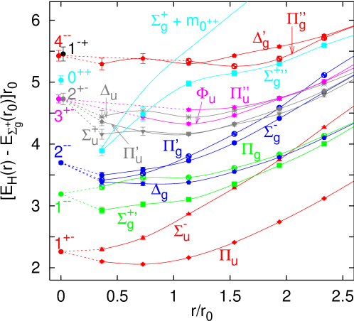
Figure 13: Different hybrid potentials Juge et al. (2003) at a lattice spacing $a_{\sigma}\approx 0.2$ fm $\approx 0.4\,r_{0}$, where $r_{0}\approx 0.5$ fm is the scale for which $-r_{0}^{2}dV/dr|_{r=r_{0}}=1.65$ Sommer (1994), in comparison with the gluelump spectrum Foster and Michael (1999) (circles, left-most data points). The gluelump spectrum has been shifted by a constant to adjust the $1^{+-}$ state with the $\Pi_{u}$ and $\Sigma_{u}^{-}$ potentials at short distance. In addition, we include the sum of the ground state ($\Sigma_{g}^{+}$) potential and the scalar glueball mass $m_{0^{++}}$ Bali et al. (1993); Morningstar and Peardon (1999); Lucini and Teper (2001). The lines are drawn to guide the eye. From Bali and Pineda (2004).

VI.2 Static pNRQCD in the weak-coupling regime

In the static limit pNRQCD has the same symmetries as NRQCD. In this section we will discuss some general properties of the short-distance behaviour of the static energies that can be straightforwardly derived within this EFT. We will follow Brambilla et al. (2000).

In the limit $\Lambda_{\rm QCD}\ll 1/r$ and at LO in $1/m$, the spectrum of the theory can be read off from the Lagrangian (61). In particular, the LO solution corresponds to the zeroth order of the multipole and $1/m$ expansions. At this order, while the singlet decouples from the octet and the gluons, the octet is still coupled to gluons. We call gluelumps the states made of an adjoint source in the presence of a gluonic field,

$$H({\bf R},{\bf r},t)\equiv H^{a}({\bf R},t)O^{a}({\bf R},{\bf r},t).$$ (201)

These, in turn, correspond to the gluonic excitations between static quarks in the short-distance limit, for which there is abundant non-perturbative data available from lattice simulations (see Fig. 13). Depending on the glue operator $H^{a}$ and its symmetries, the gluelump operator $O^{a}H^{a}$ describes a specific gluonic excitation between static quarks and its static energy, $V_{H}$.

In static pNRQCD at lowest order in the multipole expansion, besides the symmetries of static NRQCD, extra symmetries for the gluonic excitations between static quarks appear. The glue dynamics no longer involves the relative coordinate ${\bf r}$. Therefore, the glue associated with a gluonic excitation between static quarks acquires a spherical symmetry. In the centre-of-mass system, gluonic excitations between static quarks are, therefore, classified according to representations of $O(3)\otimes{\rm C}$, which we summarize by $L$, the angular momentum, CP and reflection with respect to a plane passing through the quark-antiquark axis. Since this symmetry group is larger than that of NRQCD, several gluonic excitations between static quarks are expected to be approximately degenerate in pNRQCD, i.e. in the short-distance limit $r\ll 1/\Lambda_{\rm QCD}$. We illustrate this point in Tab. 1 where all operators, $H$, up to dimension 3 are built and classified according to their quantum numbers in NRQCD and pNRQCD. In Tab. 1 all the operators are evaluated at the centre-of-mass coordinates. $\Sigma_{g}^{+}$ is not displayed since it corresponds to the singlet state. The prime indicates excited states of the same quantum numbers. The operators chosen for the $\Pi$ and $\Delta$ states are not eigenstates of the reflection operator. This is not important since these states are degenerate with respect to this symmetry. From the results of Tab. 1 the following degeneracies are expected in the short-distance limit:

$$\Sigma_{g}^{+\,\prime}\sim\Pi_{g}\;;\qquad\Sigma_{g}^{-}\sim\Pi_{g}^{\prime}\sim\Delta_{g}\,;$$

$$\Sigma_{u}^{-}\sim\Pi_{u}\;;\qquad\Sigma_{u}^{+}\sim\Pi_{u}^{\prime}\sim\Delta_{u}\,.$$ (202)

Similar observations have also been made by Foster and Michael (1999). In pNRQCD they emerge in a quite clear and straightforward way and one can explicitly write down the relevant operators. For higher excitations the expected degeneracies have been obtained by Bali and Pineda (2004). We will discuss them further when comparing with lattice data in sec. VI.4.

b

Gluelumps
$O^{a}H^{a}$	$L=1$	$L=2$
$\Sigma_{g}^{+\,\prime}$	${\bf r}\cdot{\bf E}\;,{\bf r}\cdot({\bf D}\times{\bf B})$
$\Sigma_{g}^{-}$		$({\bf r}\cdot{\bf D})({\bf r}\cdot{\bf B})$
$\Pi_{g}$	${\bf r}\times{\bf E}\;,{\bf r}\times({\bf D}\times{\bf B})$
$\Pi_{g}^{\prime}$		${\bf r}\times(({\bf r}\cdot{\bf D}){\bf B}+{\bf D}({\bf r}\cdot{\bf B}))$
$\Delta_{g}$		$({\bf r}\times{\bf D})^{i}({\bf r}\times{\bf B})^{j}+({\bf r}\times{\bf D})^{j}({\bf r}\times{\bf B})^{i}$
$\Sigma_{u}^{+}$		$({\bf r}\cdot{\bf D})({\bf r}\cdot{\bf E})$
$\Sigma_{u}^{-}$	${\bf r}\cdot{\bf B}\;,{\bf r}\cdot({\bf D}\times{\bf E})$
$\Pi_{u}$	${\bf r}\times{\bf B}\;,{\bf r}\times({\bf D}\times{\bf E})$
$\Pi_{u}^{\prime}$		${\bf r}\times(({\bf r}\cdot{\bf D}){\bf E}+{\bf D}({\bf r}\cdot{\bf E}))$
$\Delta_{u}$		$({\bf r}\times{\bf D})^{i}({\bf r}\times{\bf E})^{j}+({\bf r}\times{\bf D})^{j}({\bf r}\times{\bf E})^{i}$

Table 1: Operators $H$ for the $\Sigma$, $\Pi$ and $\Delta$ gluonic excitations between static quarks in pNRQCD up to dimensions 3. The covariant derivative is understood in the adjoint representation. ${\bf D}\cdot{\bf B}$ and ${\bf D}\cdot{\bf E}$ do not appear, the first because it is identically zero after using the Jacobi identity, while the second gives vanishing contributions after using the equations of motion. From Brambilla et al. (2000)

So far only the symmetries of pNRQCD at lowest order in the multipole expansion have been used. In fact one can go beyond that and predict the shape of the static energies by calculating the singlet and gluelump (static hybrid) correlators

$$\langle{\rm vac}|H({\bf R},{\bf r},T/2)H^{\dagger}({\bf R}^{\prime},{\bf r}^{\prime},-T/2)|{\rm vac}\rangle\sim\delta^{3}({\bf R}-{\bf R}^{\prime})\delta^{3}({\bf r}-{\bf r}^{\prime})\,e^{-iTV_{H}(r)}\,,$$ (203)

$$\langle{\rm vac}|S({\bf r},{\bf R},T/2)S^{\dagger}({\bf R}^{\prime},{\bf r}^{\prime},-T/2)|{\rm vac}\rangle\sim\delta^{3}({\bf R}-{\bf R}^{\prime})\delta^{3}({\bf r}-{\bf r}^{\prime})\,e^{-iTV_{s}^{(0)}(r)}\,,$$ (204)

for large $T$. At lowest order in the multipole expansion the spectrum of the singlet state reads

$$E_{s}(r)=2m+V_{s}^{(0)}(r)+{\cal O}(r^{2})\,.$$ (205)

For the static hybrids, the spectrum reads ($V_{H}=V_{o}^{(0)}(r)+\Lambda_{H}$)

$$E_{H}(r)=2m+V_{o}^{(0)}(r)+\Lambda_{H}+{\cal O}(r^{2})\,,$$ (206)

where

$$\Lambda_{H}\equiv\lim_{T\to\infty}\frac{i}{T}\ln\langle H^{a}(T/2)\phi_{ab}^{\rm adj}(T/2,-T/2)H^{b}(-T/2)\rangle\,.$$ (207)

Note that Eq. (207) allows us to relate the correlation length of some gluonic correlators to the behavior of the spectrum of the static hybrids at short distances. Note also that $\Lambda_{H}$ is the same for operators corresponding to states that are degenerate.

The potentials $V_{s}^{(0)}$ and $V_{o}^{(0)}$ can be computed within perturbation theory. One could then perform a detailed comparison with lattice data. We will see that in order to do so we will have to deal first with the renormalon ambiguities in the way explained in ch. V.

VI.3 The singlet static potential at short distances versus lattice

In the last years, lattice simulations Bali et al. (1997); Necco and Sommer (2002) have improved their predictions at short distances allowing very accurate comparisons between perturbation theory and lattice simulations. In order to perform this comparison, we cannot work in the on-shell scheme due to the presence of the renormalon, which destroys the convergence of the perturbative series. Therefore, schemes were introduced to make the renormalon cancellation explicit. In Sumino (2002); Recksiegel and Sumino (2002) the renormalon cancellation is achieved order by order in $\alpha_{\rm s}$ by expanding both $m$ and $V_{s}^{(0)}$ in terms of the same $\alpha_{\rm s}(\nu)$. A potential problem of this method is the appearance of large logarithms in the mass expansion. In Necco and Sommer (2001) lattice data were shown to agree with perturbation theory at short distances if the force was used instead of the potential. It was shown in Pineda (2003b) that this is equivalent to working in a renormalon-free scheme, and a first quantitative comparison of the (quenched) lattice data with the renormalon-subtracted potential $V_{s,\rm RS}^{(0)}(r)$ was done (see also Lee (2003b)). This analysis allowed to put quantitative bounds on non-perturbative effects at short distances and, in particular, it ruled out a linear potential with slope $\sigma=0.21\,{\rm GeV}^{2}$ at short distances (see also Pineda (2004)). It also showed that today lattice data are precise enough to be sensitive to three-loop perturbation theory (see Fig. 14). Overall, up to distances of around 0.4-0.5$\,r_{0}$, perturbation theory is convergent with small errors and agrees with lattice data in all of the previous analyses. For larger distances the analysis of Pineda (2003b) shows agreement with the lattice data (within errors) up to distances of $\sim 0.8\,r_{0}$ if large logarithms are resummed. In Recksiegel and Sumino (2003) it was argued that, by fine-tuning the renormalization scale, agreement with lattice data can be reached (within errors) up to $3\,r_{0}$. Nevertheless, for such large distances, the use of perturbation theory is quite doubtful. Therefore, further studies are needed to see whether this agreement is purely accidental or a theoretical explanation can be given.

Figure 14: Plot of $r_{0}(V_{\rm RS}(r)-V_{\rm RS}(r^{\prime})+E_{latt.}(r^{\prime}))$ versus r at tree (dashed line), one-loop (dash-dotted line), two-loop (dotted line) and three-loop level (estimate) plus the RG expression for the US logarithms (solid line) compared with the lattice simulations $E_{latt.}(r)$ Necco and Sommer (2002). For the scale of $\alpha_{\rm s}(\nu)$, we set $\nu=1/r$. Further, $\nu_{f}=\nu_{us}=2.5\,r_{0}^{-1}$, $\Lambda_{\overline{\rm MS}}=0.602\,r_{0}^{-1}$ Capitani et al. (1999), and $r^{\prime}=0.15399\,r_{0}$. From Pineda (2003b).

VI.4 Gluelumps versus lattice

We compare the predictions of pNRQCD for the static hybrids in the weak-coupling regime with lattice data. We first explore at which distances the expected degeneracies start to be fulfilled and whether the gluelump mass and hybrid potential splittings agree with each other. See Fig. 13. On a qualitative level the short-distance data are consistent with the expected degeneracies. In any case, at best, one can possibly imagine perturbation theory to be valid for the left-most two data points. With the exception of the $\Pi_{u}$, $\Pi_{u}^{\prime}$ and $\Phi_{u}$ potentials there are also no clear signs for the onset of the short-distance $1/r$ behaviour with a positive coefficient as expected from perturbation theory. Furthermore, most of the gaps within multiplets of hybrid potentials, which at LO depend on the size of the non-perturbative $r^{2}$ term, are still quite significant, even at $r=0.4\,r_{0}$; for instance, the difference between the $\Sigma_{u}^{-}$ and $\Pi_{u}$ potentials at this distance is about 0.28 $r_{0}^{-1}\approx 110$ MeV.

From the above considerations it is clear that for a more quantitative study one needs lattice data at shorter distances. These have been provided by Bali and Pineda (2004) for the lowest two gluonic excitations, $\Pi_{u}$ and $\Sigma_{u}^{-}$. We display their differences in the continuum limit in Fig. 15. We see how these approach zero at small $r$, as expected from the short-distance expansion. pNRQCD predicts that the next effects should be of ${\cal O}(r^{2})$ (and renormalon-free). The lattice data are fitted rather well by a $\Delta E_{\Pi_{u}-\Sigma_{g}^{+}}=A_{\Pi_{u}-\Sigma_{u}^{-}}r^{2}$ ansatz for short distances, with slope (see Fig. 15),

$$A_{\Pi_{u}-\Sigma_{u}^{-}}=0.92^{+0.53}_{-0.52}\,r_{0}^{-3}\,,$$ (208)

where the error is purely statistical (lattice), the systematic error being negligible. We remark that within the framework of static pNRQCD and to second order in the multipole expansion, one can relate the slope $A_{\Pi_{u}-\Sigma_{u}^{-}}$ to gluonic correlators of QCD.

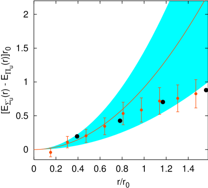
Figure 15: Splitting between the $\Sigma_{u}^{-}$ and the $\Pi_{u}$ potentials, extrapolated to the continuum limit, and comparison with a quadratic fit to the $r{\ \lower-1.2pt\vbox{\hbox{\hbox to0.0pt{$<$\hss}\lower 6.0pt\vbox{\hbox{$\sim$}}}}\ }0.5\,r_{0}$ data points ($r_{0}^{-1}\approx 0.4$ GeV). The big circles correspond to the data of Juge et al. (2003). The errors in this case are smaller than the symbols. The smaller circles correspond to the data of Bali and Pineda (2004). From Bali and Pineda (2004).

One can go beyond these analyses and use lattice data plus the knowledge of the (perturbative) octet potential to obtain numerical values for gluelump masses in a particular scheme. However, analogously to the situation with the static singlet potential, the convergence of the perturbative series of the octet potential is bad. The solution to this problem comes again from working in a RS scheme properly generalized to the hybrid case. The hybrid energy reads

$$E_{H}(r)=2m_{\rm RS}(\nu_{f})+V_{o,\rm RS}(r;\nu_{f})+\Lambda_{H}^{\rm RS}(\nu_{f})+{\cal O}(r^{2})\,.$$ (209)

In the RS scheme the octet potential reads

$$V_{o,\rm RS}(\nu_{f})=V_{o}-\delta V_{o,\rm RS}=\sum_{n=0}^{\infty}V^{\rm RS}_{o,n}\alpha_{\rm s}^{n+1}\,,$$ (210)

where

$$\delta V_{o,\rm RS}=\sum_{n=1}^{\infty}N_{V_{o}}\,\nu_{f}\,\left({\beta_{0}\over 2\pi}\right)^{n}\alpha_{\rm s}^{n+1}(\nu_{f})\sum_{k=0}^{\infty}c_{k}{\Gamma(n+1+b-k)\over\Gamma(1+b-k)}\,.$$ (211)

This specifies the gluelump mass which reads

$$\Lambda_{H}^{\rm RS}(\nu_{f})=\Lambda_{H}-\delta\Lambda_{\rm RS}(\nu_{f}),$$ (212)

where

$$\delta\Lambda_{\rm RS}(\nu_{f})=\sum_{n=1}^{\infty}N_{\Lambda}\,\nu_{f}\,\left({\beta_{0}\over 2\pi}\right)^{n}\alpha_{\rm s}^{n+1}(\nu_{f})\sum_{k=0}^{\infty}c_{k}{\Gamma(n+1+b-k)\over\Gamma(1+b-k)}\,.$$ (213)

Note that factorization requires

$$2N_{m}+N_{V_{o}}+N_{\Lambda}=0.$$ (214)

$N_{m}$ is already known and $N_{V_{o}}$ can also be obtained approximately from low orders in perturbation theory following the same procedure as in sec. V.1. One now has a convergent series in perturbation theory and can obtain absolute values for the masses of the gluelumps, in particular for the lowest gluelump using the splitting of the $\Sigma_{g}^{+}$ and the $\Pi_{u}$ potential. Then using the lattice data of Foster and Michael (1999), it is possible to obtain the absolute values for the masses of all gluelump excitations in a given scheme (in this case, the RS scheme). The results are summarized in Table 2. For a comparison with other determinations, see Bali and Pineda (2004).

Table 2: Absolute values for the gluelump masses in the continuum limit in the RS scheme at $\nu_{f}=2.5\,r_{0}^{-1}\approx 1$ GeV, in $r_{0}$ units and in GeV. Note that an additional uncertainty of about 10% should be added to the last column to account for the quenched approximation. We also display examples of creation operators $H$ for these states. The curly braces denote complete symmetrization of the indices. From Bali and Pineda (2004)

$J^{PC}$	$H$	$\Lambda_{H}^{\rm RS}r_{0}$	$\Lambda_{H}^{\rm RS}$/GeV
$1^{+-}$	$B_{i}$	2.25(39)	0.87(15)
$1^{--}$	$E_{i}$	3.18(41)	1.25(16)
$2^{--}$	$D_{\{i}B_{j\}}$	3.69(42)	1.45(17)
$2^{+-}$	$D_{\{i}E_{j\}}$	4.72(48)	1.86(19)
$3^{+-}$	$D_{\{i}D_{j}B_{k\}}$	4.72(45)	1.86(18)
$0^{++}$	${\mathbf{B}}^{2}$	5.02(46)	1.98(18)
$4^{--}$	$D_{\{i}D_{j}D_{k}B_{l\}}$	5.41(46)	2.13(18)
$1^{-+}$	$({\mathbf{B}}\wedge{\mathbf{E}})_{i}$	5.45(51)	2.15(20)

VII Potential NRQCD. The strong-coupling regime

In this chapter, we discuss pNRQCD under the condition that $\Lambda_{\rm QCD}\gg E$. We have called this situation the strong-coupling regime of pNRQCD in ch. III, where some general features of the physical picture have already been discussed. Since the EFT does not tell us anything about the non-perturbative dynamics of QCD, we have to rely on some assumptions in order to identify the relevant degrees of freedom. The assumptions will be minimal, supported by general considerations and lattice data, but clearly we are on a less solid ground here than in the weak-coupling regime.

VII.1 Degrees of freedom

If we consider the case without light quarks, the physical states made by a heavy quark and antiquark are heavy quarkonium states or hybrids or both of them in the presence of glueballs. Quenched lattice data show that the static energy of the lowest state is separated by a gap of order $\Lambda_{\rm QCD}$ from the higher ones. This feature is preserved in going to unquenched simulations (see Fig. 4). We assume that this feature is also preserved in the dynamical case of heavy quarks with finite masses. This leads to identify the heavy quarkonium with the solution of the Schrödinger equation on which the static potential corresponds to the ground state static energy.

Once light fermions have been incorporated, however, new gauge-invariant states appear besides the heavy quarkonium, hybrids and glueballs. First, we have states with no heavy quark content. Due to chiral symmetry, there is a mass gap, of ${\cal O}(\Lambda_{\rm QCD})$, between the Goldstone bosons, which are massless in the chiral limit, and the rest of the spectrum. Therefore, the Goldstone bosons are US degrees of freedom, while the rest of the spectrum is integrated out at the scale $\Lambda_{\rm QCD}$. Besides these, we also have bound states made of one heavy quark and light quarks. In practice, we are considering the $Q\bar{q}$–$\bar{Q}q$ system. The energy of this system is, according to the HQET counting rules Neubert (1994), $m_{Q\bar{q}}+m_{\bar{Q}q}=2m+2\,{\bar{\Lambda}}$. Therefore, since ${\bar{\Lambda}}\sim\Lambda_{\rm QCD}$, we assume that also these states are integrated out at the scale $\Lambda_{\rm QCD}$. This cannot be done for heavy quarkonium states near threshold, since in this case there is no mass gap between the heavy quarkonium and the creation of a $Q\bar{q}$–$\bar{Q}q$ pair. Thus, if we want to study the heavy quarkonium near threshold, we should include these degrees of freedom in the spectrum (for a model-dependent approach to this situation see, for instance, Eichten et al. (1978)). We will assume here that the considered heavy quarkonium states are safely far from threshold.

Summarizing, the degrees of freedom of pNRQCD in the regime $\Lambda_{\rm QCD}\gg E$ for quarkonium states far from threshold are a singlet field $S$, describing the heavy quarkonium state, and Goldstone boson fields. In the following, we will not consider the Goldstone boson fields. If one switches off the light fermions, only the singlet survives and pNRQCD reduces to a pure two-particle NR quantum-mechanical system, usually referred to as a pure potential model.

VII.2 Power counting

The structure of the pNRQCD Lagrangian under the above conditions is very simple: it is just a bilinear in the singlet field. Therefore, establishing the power counting means to estimate the size of the terms multiplying the bilinear.

The soft scale $|{\bf p}|$ must be assigned to $-i\mbox{\boldmath$\nabla$}_{\bf r}$ and $1/r$, the US scale $E\sim{\bf p}^{2}/m$ to the time derivatives $i\partial_{0}$ and $V_{s}^{(0)}$. This last condition follows from the consistency of the theory that requires the virial theorem to be fulfilled. In other words, all the terms in the Schrödinger equation,

$$i\partial_{0}\phi=E\,\phi=({\bf p}^{2}/m+V_{s}^{(0)})\phi,$$ (215)

must count the same. Note that the normalization condition of the wavefunction ($\int d^{3}{\bf r}\,|\phi({\bf r})|^{2}=1$) sets $|\phi|^{2}\sim|{\bf p}|^{3}$. In general, the $1/m$ corrections to the potential (real and imaginary) will be a combination of $\alpha_{\rm s}$ calculated at different scales, derivatives with respect to the relative coordinate $-i\mbox{\boldmath$\nabla$}_{\bf r}$, $1/r$ and expectation values of the fields of the light degrees of freedom. The quantities $m$ and $\alpha_{\rm s}(m)$ are inherited from the hard matching and have well-known values, in particular $\alpha_{\rm s}(m)\ll 1$. The strong-coupling constant also appears evaluated at the scales $\sqrt{m\,\Lambda_{\rm QCD}}$, $1/r$, $\Lambda_{\rm QCD}$ and $E$. At the scale $\sqrt{m\,\Lambda_{\rm QCD}}$, which appears in loop calculations (see below), $\alpha_{\rm s}(m)\ll\alpha_{\rm s}(\sqrt{m\,\Lambda_{\rm QCD}})\ll 1$ since $\sqrt{m\,\Lambda_{\rm QCD}}\gg\Lambda_{\rm QCD}$. At the scales $\Lambda_{\rm QCD}$ and $E$, $\alpha_{\rm s}(\Lambda_{\rm QCD})\sim 1$ and $\alpha_{\rm s}(E)\sim 1$ by definition of the strong-coupling regime. If $|{\bf p}|\sim\Lambda_{\rm QCD}$, then also $\alpha_{\rm s}(1/r)\sim 1$. If $|{\bf p}|\gg\Lambda_{\rm QCD}\gg E$, then $\alpha_{\rm s}(\sqrt{m\,\Lambda_{\rm QCD}})\ll\alpha_{\rm s}(1/r)\ll 1$. In the situation $|{\bf p}|\sim\Lambda_{\rm QCD}$ the expectation values of the fields of the light degrees of freedom depend on ${\bf r}$ and $\Lambda_{\rm QCD}$, while in the situation $|{\bf p}|\gg\Lambda_{\rm QCD}\gg E$, the $1/r\sim|{\bf p}|$ dependence factorizes and the expectation values of the fields of the light degrees of freedom depend only on $\Lambda_{\rm QCD}$. In both cases their natural counting is $\Lambda_{\rm QCD}$ to the power of their dimension.

VII.3 Lagrangian and symmetries

The pNRQCD Lagrangian (without Goldstone bosons) is given by:

$$L_{\rm pNRQCD}=\int d^{3}{\bf R}\int d^{3}{\bf r}\;S^{\dagger}\big{(}i\partial_{0}-h_{s}({\bf x}_{1},{\bf x}_{2},{\bf p}_{1},{\bf p}_{2},{\bf S}_{1},{\bf S}_{2})\big{)}S,$$ (216)

where

$$h_{s}({\bf x}_{1},{\bf x}_{2},{\bf p}_{1},{\bf p}_{2},{\bf S}_{1},{\bf S}_{2})={{\bf p}_{1}^{2}\over 2m_{1}}+{{\bf p}_{2}^{2}\over 2m_{2}}+V_{s}({\bf x}_{1},{\bf x}_{2},{\bf p}_{1},{\bf p}_{2},{\bf S}_{1},{\bf S}_{2}),$$ (217)

${\bf p}_{j}=-i\mbox{\boldmath$\nabla$}_{{\bf x}_{j}}$, ${\bf r}={\bf x}_{1}-{\bf x}_{2}$, ${\bf R}=({\bf x}_{1}+{\bf x}_{2})/2$ and ${\bf S}_{j}$ is the spin operator of particle $j$. In the following, as long as not stated differently, we will assume $m_{1}\neq m_{2}$. However, we will not exploit a possible hierarchy between the two masses, which, for our purpouses, are of the same order $\sim m\gg\Lambda_{\rm QCD}$. The potential $V_{s}$ contains a real and an imaginary part. The real part is responsible for the binding, the imaginary part for the decay width of the heavy quarkonium state. The imaginary part of $V_{s}$ comes from the imaginary parts of the matching coefficients of the 4-fermion operators of NRQCD. The potential $V_{s}$ is, in general, a non-perturbative quantity, even if, to some degree, it may contain pieces calculable in perturbation theory, like, for instance, the matching coefficients of NRQCD, or in general any contribution coming from scales larger than $\Lambda_{\rm QCD}$. It is the aim of the matching procedure, which we will discuss in the following sections, to provide the factorization formulas and the exact expressions for the non-perturbative pieces. These may be eventually calculated on the lattice or in QCD vacuum models, which will be the subject of sec. VII.7.

The symmetries of the singlet field are those already discussed for the pNRQCD Lagrangian in the weak-coupling regime. In particular, the potential and the kinetic energies satisfy the Poincaré invariance constraints (86) and (87) (for the singlet potential). Note that Poincaré invariance may also constrain the natural power counting discussed in sec. VII.2.

VII.4 Matching: analytic and non-analytic mass terms

Despite the fact that the strong-coupling Lagrangian (216) looks quite simple, the matching procedure that leads to it may be complicated. This is due to the fact that we have to integrate out, and, therefore, to make explicit, all the degrees of freedom (or momentum regions) that appear in the range from the hard to the US scale within a non-perturbative environment.

b

Figure 16: The incoming energy $E$ is of order $\Lambda_{\rm QCD}$, $p$ and $q$ of order $mv$. The vertex describes the interaction with an external potential $V$.

Since we are also integrating out $\Lambda_{\rm QCD}$, new momentum regions (apart from $\Lambda_{\rm QCD}$ itself) that do not appear in the weak-coupling matching show up. Let us consider, for instance, the diagram of Fig. 16. Suppose that the incoming (outcoming) particle is an off-shell particle of energy $\sim\Lambda_{\rm QCD}$ and three-momentum $p(q)\sim mv$ (for instance, an on-shell particle that just emitted (absorbed) a soft gluon of energy $\Lambda_{\rm QCD}$). The diagram corresponds to the integral:

$$\int{d^{3}\mbox{\boldmath$\xi$}\over(2\pi)^{3}}V({\bf p}-\mbox{\boldmath$\xi$}){1\over E-{\mbox{\boldmath$\xi$}^{2}/m}+i\epsilon}V(\mbox{\boldmath$\xi$}-{\bf q}).$$ (218)

This integral also receives a contribution from the three-momentum region $\xi\sim\sqrt{m\,E}\sim\sqrt{m\,\Lambda_{\rm QCD}}$. Since $\sqrt{m\,\Lambda_{\rm QCD}}\gg\Lambda_{\rm QCD}$, the potential is perturbative, and since $\sqrt{m\,\Lambda_{\rm QCD}}\gg p,q$, we may expand in $p$ and $q$ and the integral effectively reduces to:

$$\alpha_{\rm s}^{2}\int{d^{3}\mbox{\boldmath$\xi$}\over(2\pi)^{3}}{1\over\xi^{4}}{1\over E-{\mbox{\boldmath$\xi$}^{2}/m}+i\epsilon}\sim\alpha_{\rm s}^{2}{1\over\Lambda_{\rm QCD}}{1\over\sqrt{m\,\Lambda_{\rm QCD}}},$$ (219)

where $\alpha_{\rm s}$ is calculated at the (perturbative) scale $\sqrt{m\,\Lambda_{\rm QCD}}$. From the above example we may draw the following conclusions. First, in the strong-coupling regime new degrees of freedom show up in loops, namely quark-antiquark pairs with relative three-momentum of order $\sqrt{m\,\Lambda_{\rm QCD}}$ and on-shell energy of order $\Lambda_{\rm QCD}$. Since the scale $\sqrt{m\,\Lambda_{\rm QCD}}\gg|{\bf p}|$ for $\Lambda_{\rm QCD}\gg E$, this is the largest scale below $m$ and, thus, the first to be integrated out. The only reason this otherwise dominant contribution to the potential is suppressed is that it appears only in loops. Second, since we expand in the external momenta, which are small compared to $\sqrt{m\,\Lambda_{\rm QCD}}$, the effective interaction that arises is local. Third, this kind of contribution is non-analytic in $m$.

It is convenient to split the potential (imaginary and real part) into a part that gets contributions only from scales that are analytic in the mass, $V^{1/m}$, and another, $V^{1/\sqrt{m}}$, that contains any contribution coming from the scale $\sqrt{m\,\Lambda_{\rm QCD}}$:

$$V_{s}=V^{1/m}+V^{1/\sqrt{m}}.$$ (220)

We will often refer to $V^{1/\sqrt{m}}$ as the part of the potential that is non-analytic in $1/m$. This is only true at LO, which is, however, the order at which we will work here. The matching for the $V^{1/m}$ part may be performed in a strict $1/m$ expansion. The matching for the $V^{1/\sqrt{m}}$ part maybe done by integrating out quark-antiquark pairs with relative three-momenta of order $\sqrt{m\,\Lambda_{\rm QCD}}$.

We will next discuss the matching procedures for $V^{1/m}$ and $V^{1/\sqrt{m}}$ in the situations $|{\bf p}|\sim\Lambda_{\rm QCD}$ and $|{\bf p}|\gg\Lambda_{\rm QCD}\gg E$. We will first consider the case $|{\bf p}|\sim\Lambda_{\rm QCD}$ in sec. VII.5. The potential will be a function of ${\bf r}$ and $\Lambda_{\rm QCD}$. This is the most general case. The particular case $|{\bf p}|\gg\Lambda_{\rm QCD}\gg E$ may be derived from it by factorizing the potential in a high-energy part that depends on $1/r\sim|{\bf p}|$ and a low-energy part that depends on $\Lambda_{\rm QCD}$. In this case, however, it is more practical and consistent with the general philosophy of the EFT to achieve factorization directly by integrating out the scales $|{\bf p}|$ and $\Lambda_{\rm QCD}$ in two different steps of the matching procedure. We will consider this situation in sec. VII.6. We note here that terms that come out local in the situation $|{\bf p}|\sim\Lambda_{\rm QCD}$ are already factorized and, therefore, will be reproduced (up to field redefinitions) in the situation $|{\bf p}|\gg\Lambda_{\rm QCD}\gg E$. This is the case of the imaginary part of the potential, which comes from the 4-fermion contact terms of the NRQCD Lagrangian, and the part of the potential that is non-analytic in $1/m$.

Finally, we would like to mention that soft light fermions will not be explicitly considered in the matching computation. If we want to incorporate them, the procedure would be analogous. One would have to consider the matrix elements and Wilson loops with dynamical light fermions incorporated and new terms appearing in the energies at ${\cal O}(1/m^{2})$ due to operators involving light fermions that appear in the NRQCD Lagrangian at ${\cal O}(1/m^{2})$ and the Gauss law.

VII.5 Matching for $|{\bf p}|\sim\Lambda_{\rm QCD}$

In sec. VI.1, we have discussed the static limit of NRQCD. The spectrum consists of the static energies $E_{0}^{(0)}\ll E_{1}^{(0)}\ll\dots$. We assume a gap of order $\Lambda_{\rm QCD}$ between $E_{0}^{(0)}$ and the higher excitations. pNRQCD is, by definition, the EFT that describes the lowest excitation of the NRQCD spectrum. From Eq. (216), it follows that pNRQCD in the static limit consists of a singlet field $S$ with static energy $V^{(0)}$. Since the static energy is an observable, the matching condition in the static limit is:

$$E_{0}^{(0)}(r)=V^{(0)}(r).$$ (221)

Note that the left-hand side is a quantity defined in NRQCD, while the right-hand side is a matching coefficient of pNRQCD.

We may think of generalizing the matching condition (221) to the non-static case. Similarly to what we have done in sec. VI.1, we introduce the normalized eigenstates, $|\underline{n};{\bf x}_{1},{\bf x}_{2}\rangle$, and eigenvalues, $E_{n}({\bf x}_{1},{\bf x}_{2};{\bf p}_{1},{\bf p}_{2})$, of the full NRQCD Hamiltonian $H$. They satisfy the equations

$$H|\underline{n};{\bf x}_{1},{\bf x}_{2}\rangle=\int d^{3}x_{1}^{\prime}d^{3}x_{2}^{\prime}|\underline{n};{\bf x}_{1}^{\prime},{\bf x}_{2}^{\prime}\rangle E_{n}({\bf x}_{1}^{\prime},{\bf x}_{2}^{\prime},{\bf p}_{1}^{\prime},{\bf p}_{2}^{\prime},{\bf S}_{1},{\bf S}_{2})\delta^{(3)}({\bf x}_{1}^{\prime}-{\bf x}_{1})\delta^{(3)}({\bf x}_{2}^{\prime}-{\bf x}_{2}),$$

(222)

$$\langle\underline{m};{\bf x}_{1},{\bf x}_{2}|\underline{n};{\bf y}_{1},{\bf y}_{2}\rangle=\delta_{nm}\delta^{(3)}({\bf x}_{1}-{\bf y}_{1})\delta^{(3)}({\bf x}_{2}-{\bf y}_{2}),$$ (223)

where the states are labeled with the positions ${\bf x}_{1}$ and ${\bf x}_{2}$ of the static solution even if the position operator does not commute with $H$ beyond the static limit. The eigenvalues $E_{n}$ are, in general, functions of the momentum and spin operators and, therefore, should be understood as operators as well. We assume a gap of order $\Lambda_{\rm QCD}$ between (the levels of) $E_{0}$ and (the levels of) $E_{n}$ for $n>0$. Under this circumstance, and arguing as in the static case above, it follows that the matching condition reads:

$$E_{0}({\bf x}_{1},{\bf x}_{2},{\bf p}_{1},{\bf p}_{2},{\bf S}_{1},{\bf S}_{2})=h_{s}({\bf x}_{1},{\bf x}_{2},{\bf p}_{1},{\bf p}_{2},{\bf S}_{1},{\bf S}_{2}).$$ (224)

Again, this equation expresses the (real and imaginary parts of the) pNRQCD Hamiltonian in terms of a quantity,

$$E_{0}({\bf x}_{1},{\bf x}_{2},{\bf p}_{1},{\bf p}_{2},{\bf S}_{1},{\bf S}_{2})\delta^{(3)}({\bf x}_{1}-{\bf y}_{1})\delta^{(3)}({\bf x}_{2}-{\bf y}_{2})=\langle\underline{0};{\bf x}_{1},{\bf x}_{2}|H|\underline{0};{\bf y}_{1},{\bf y}_{2}\rangle,$$ (225)

defined in NRQCD. The aim of the matching is to calculate this quantity. As discussed above, it will contain a part that is analytic in $1/m$ and another that is not.

VII.5.1 Matching of the analytic terms: quantum-mechanical matching

The analytic part of $E_{0}$ can be calculated, by definition, in a strict $1/m$ expansion. The idea is to split the NRQCD Hamiltonian as

$$H=H^{(0)}+H_{I},$$ (226)

where $H^{(0)}$ is the static Hamiltonian, whose eigenstates and eigenvalues have been discussed in sec. VI.1, and

$$H_{I}={H^{(1,0)}\over m_{1}}+{H^{(0,1)}\over m_{2}}+{H^{(2,0)}\over m_{1}^{2}}+{H^{(0,2)}\over m_{2}^{2}}+{H^{(1,1)}\over m_{1}m_{2}}+\cdots\;.$$ (227)

is the sum of all higher-order terms in the $1/m$ expansion of the NRQCD Hamiltonian. Then solve Eq. (222) by doing quantum-mechanic perturbation theory around the static solution. Calculated in this way, the eigenstates (and eigenvalues) of Eq. (222) come out as expansions in powers of $1/m$:

$$|\underline{n};{\bf x}_{1},{\bf x}_{2}\rangle=|\underline{n};{\bf x}_{1},{\bf x}_{2}\rangle^{(0)}+{1\over m_{1}}|\underline{n};{\bf x}_{1},{\bf x}_{2}\rangle^{(1,0)}+{1\over m_{2}}|\underline{n};{\bf x}_{1},{\bf x}_{2}\rangle^{(0,1)}$$

$$~{}~{}~{}~{}~{}~{}~{}~{}~{}~{}~{}~{}+{1\over m_{1}^{2}}|\underline{n};{\bf x}_{1},{\bf x}_{2}\rangle^{(2,0)}+{1\over m_{2}^{2}}|\underline{n};{\bf x}_{1},{\bf x}_{2}\rangle^{(0,2)}+{1\over m_{1}m_{2}}|\underline{n};{\bf x}_{1},{\bf x}_{2}\rangle^{(1,1)}+\cdots\;.$$ (228)

A complete derivation can be found in the original literature Brambilla et al. (2001b); Pineda and Vairo (2001); Brambilla et al. (2003a). Here we only make a few remarks. First, the expressions for $|\underline{n};{\bf x}_{1},{\bf x}_{2}\rangle^{(1,0)}$ and $|\underline{n};{\bf x}_{1},{\bf x}_{2}\rangle^{(2,0)}$ look symilar to the well-known formulas of time-independent perturbation theory in quantum mechanics, the only difference being the fact that the energies $E_{n}^{(0)}$ depend on spatial coordinates and that the matrix elements of $H^{(1,0)}$ and $H^{(2,0)}$ are operators in the quantum-mechanical sense. Second, as usually done in quantum mechanics, we have set the relative phase between $|\underline{n};{\bf x}_{1},{\bf x}_{2}\rangle$ and $|\underline{n};{\bf x}_{1},{\bf x}_{2}\rangle^{(0)}$ to $1$ in Eq. (228). This choice is arbitrary. The freedom of choice reflects the fact that the eigenvalues and eigenstates solution of Eq. (222) are defined up to a unitary transformation $e^{iO_{n}}$ (with $O_{n}^{\dagger}=O_{n}$):

$$|\underline{n},{\bf x}_{1},{\bf x}_{2}\rangle\rightarrow\int d^{3}{\bf x}^{\prime}_{1}\,d^{3}{\bf x}^{\prime}_{2}\,|\underline{n},{\bf x}^{\prime}_{1},{\bf x}^{\prime}_{2}\rangle e^{iO_{n}({\bf x}^{\prime}_{1},{\bf x}^{\prime}_{2},{\bf p}^{\prime}_{1},{\bf p}^{\prime}_{2},{\bf S}_{1},{\bf S}_{2})}\delta^{(3)}({\bf x}^{\prime}_{1}-{\bf x}_{1})\delta^{(3)}({\bf x}^{\prime}_{2}-{\bf x}_{2}),$$ (229)

$$E_{n}({\bf x}_{1},{\bf x}_{2},{\bf p}_{1},{\bf p}_{2},{\bf S}_{1},{\bf S}_{2})\rightarrow$$

$$\qquad\int d^{3}{\bf x}^{\prime}_{1}\,d^{3}{\bf x}^{\prime}_{2}\,e^{iO_{n}({\bf x}^{\prime}_{1},{\bf x}^{\prime}_{2},{\bf p}^{\prime}_{1},{\bf p}^{\prime}_{2},{\bf S}_{1},{\bf S}_{2})}E_{n}({\bf x}_{1}^{\prime},{\bf x}_{2}^{\prime},{\bf p}_{1}^{\prime},{\bf p}_{2}^{\prime},{\bf S}_{1},{\bf S}_{2})e^{-iO_{n}({\bf x}^{\prime}_{1},{\bf x}^{\prime}_{2},{\bf p}^{\prime}_{1},{\bf p}^{\prime}_{2},{\bf S}_{1},{\bf S}_{2})}$$

$$~{}~{}~{}~{}~{}~{}~{}~{}~{}~{}~{}~{}~{}~{}~{}~{}~{}~{}~{}~{}~{}~{}~{}~{}~{}~{}~{}~{}~{}~{}~{}~{}~{}~{}~{}~{}~{}~{}~{}~{}~{}~{}~{}~{}\times\delta^{(3)}({\bf x}^{\prime}_{1}-{\bf x}_{1})\delta^{(3)}({\bf x}^{\prime}_{2}-{\bf x}_{2}).$$ (230)

Our choice preserves the power counting and allows us to obtain rather compact expressions for the potentials. Third, from the expression for the state $|\underline{0};{\bf x}_{1},{\bf x}_{2}\rangle$, the expression for the energy $E_{0}$ may be derived straightforwardly, order by order in $1/m$, from Eq. (225). Finally, the matching condition (224) gives the pNRQCD Hamiltonian.

In order to transform the quantum-mechanical expressions into expressions that only contain expectation values of gluon fields, the following steps are necessary.

(1) The first step is to integrate out the fermion fields. They appear in the matrix elements of $H^{(1)}$ and $H^{(2)}$ either in the states (see Eq. (198)) or in the Hamiltonian itself as 2- or 4-fermion interaction terms. In the first case, we have, for instance,

$${}^{(0)}\langle\underline{n};{\bf x}_{1},{\bf x}_{2}|\;\int d^{3}\mbox{\boldmath$\xi$}\;\psi^{\dagger}(\mbox{\boldmath$\xi$})\,O(\mbox{\boldmath$\xi$})\,\psi(\mbox{\boldmath$\xi$})\;|\underline{m};{\bf y}_{1},{\bf y}_{2}\rangle^{(0)}=$$

$$~{}~{}~{}~{}~{}~{}~{}~{}~{}~{}{}^{(0)}\langle n;{\bf x}_{1},{\bf x}_{2}|O({\bf x}_{1})|m;{\bf x}_{1},{\bf x}_{2}\rangle^{(0)}\;\delta^{(3)}({\bf x}_{1}-{\bf y}_{1})\delta^{(3)}({\bf x}_{2}-{\bf y}_{2}),$$ (231)

in the second case

$${}^{(0)}\langle\underline{n};{\bf x}_{1},{\bf x}_{2}|\;\int d^{3}\mbox{\boldmath$\xi$}\;\psi^{\dagger}(\mbox{\boldmath$\xi$})\,O_{A}(\mbox{\boldmath$\xi$})\,\psi(\mbox{\boldmath$\xi$})\,\chi^{\dagger}_{c}(\mbox{\boldmath$\xi$})\,O_{B}(\mbox{\boldmath$\xi$})\,\chi_{c}(\mbox{\boldmath$\xi$})\;|\underline{m};{\bf y}_{1},{\bf y}_{2}\rangle^{(0)}=$$ (232)

$$~{}~{}~{}\delta^{(3)}({\bf x}_{1}-{\bf x}_{2})\;{}^{(0)}\langle n;{\bf x}_{1},{\bf x}_{2}|O_{A}({\bf x}_{1})\,O_{B}({\bf x}_{2})|m;{\bf x}_{1},{\bf x}_{2}\rangle^{(0)}\;\delta^{(3)}({\bf x}_{1}-{\bf y}_{1})\delta^{(3)}({\bf x}_{2}-{\bf y}_{2}),$$

where $O$, $O_{A}$ and $O_{B}$ are combinations of gluon fields. In the last case, the interaction is local ($\sim\delta^{(3)}({\bf r})$). At this stage, the expressions only contain matrix elements of gluon fields on the pure gluonic states $|n;{\bf x}_{1},{\bf x}_{2}\rangle^{(0)}\equiv|n\rangle^{(0)}$. At this point, it is also possible to use the Gauss law (197). It allows us to write all the terms of the type $[{\bf D},g{\bf E}]$ in terms of $\delta^{(3)}({\bf r})$ times some color matrices, up to terms proportional to $\delta^{(3)}({\bf 0})$ that vanish in DR. We will assume to be working in this regularization scheme from now on.

(2) Further simplifications may be achieved using the identities ($F_{1,2}\equiv F({\bf x}_{1,2})$):

$${}^{\,\,(0)}\langle n|{\bf D}_{1}|n\rangle^{(0)}=\mbox{\boldmath$\nabla$}_{1},\qquad\qquad\qquad{}^{\,\,(0)}\langle n|{\bf D}_{c\,2}|n\rangle^{(0)}=\mbox{\boldmath$\nabla$}_{2},$$ (233)

$${}^{\,\,(0)}\langle n|{\bf D}_{1}|j\rangle^{(0)}={{}^{\,\,(0)}\langle n|g{\bf E}_{1}|j\rangle^{(0)}\over E_{n}^{(0)}-E_{j}^{(0)}},\quad{}^{\,\,(0)}\langle n|{\bf D}_{c\,2}|j\rangle^{(0)}=-{{}^{\,\,(0)}\langle n|g{\bf E}^{T}_{2}|j\rangle^{(0)}\over E_{n}^{(0)}-E_{j}^{(0)}}~{}\forall\,n\neq j,$$ (234)

$${}^{\,\,(0)}\langle n|g{\bf E}_{1}|n\rangle^{(0)}=-(\mbox{\boldmath$\nabla$}_{1}E_{n}^{(0)}),\qquad~{}{}^{\,\,(0)}\langle n|g{\bf E}^{T}_{2}|n\rangle^{(0)}=(\mbox{\boldmath$\nabla$}_{2}E_{n}^{(0)}),$$ (235)

where ${\bf D}_{c}$ is the charge conjugate of ${\bf D}$. The first equality follows from symmetry considerations, the second and the third may be derived from ${}^{\,\,(0)}\langle n|[H^{(0)},{\bf D}]|j\rangle^{(0)}=E_{n}^{(0)}{}^{\,\,(0)}\langle n|{\bf D}|j\rangle^{(0)}-{}^{\,\,(0)}\langle n|{\bf D}|j\rangle^{(0)}E_{j}^{(0)}$ and the canonical commutation relations.

(3) The last step consists in rewriting the quantum-mechanical expressions in terms of Wilson-loop amplitudes. We proceed in the following way. We consider an interpolating state (in the Heisenberg representation) that has a non-vanishing overlap with the ground state:

$$\psi^{\dagger}({\bf x}_{1})\phi({\bf x}_{1},{\bf x}_{2})\chi_{c}^{\dagger}({\bf x}_{2})|\hbox{vac}\rangle,$$ (236)

where $\phi$ may be everything that makes the above state overlap with the ground state $|\underline{0};{\bf x}_{1},{\bf x}_{2}\rangle^{(0)}$. We will use here the popular choice (108), which assumes that the ground state has the $\Sigma_{g}^{+}$ quantum numbers. We also define $\phi({\bf y},{\bf x};t=0)\equiv\phi({\bf y},{\bf x})$. Then we have

$$\psi^{\dagger}({\bf x}_{1})\phi({\bf x}_{1},{\bf x}_{2})\chi_{c}^{\dagger}({\bf x}_{2})|\hbox{vac}\rangle=\sum_{n}a_{n}({\bf x}_{1},{\bf x}_{2})|\underline{n};{\bf x}_{1},{\bf x}_{2}\rangle^{(0)},$$ (237)

or, without fermion fields,

$$\phi({\bf x}_{1},{\bf x}_{2})|\hbox{vac}\rangle=\sum_{n}a_{n}({\bf x}_{1},{\bf x}_{2})|n;{\bf x}_{1},{\bf x}_{2}\rangle^{(0)},$$ (238)

with $a_{0}\neq 0$. At this point, we define the Wilson-loop average $\langle\cdots\rangle_{\Box}\equiv\langle\cdots W_{\Box}\rangle$. The gauge fields are, in general, localized on the static quark lines of the Wilson loop. Therefore, $\langle\cdots\rangle_{\Box}$ is gauge invariant. Inserting the identity operator $\sum|n\rangle^{(0)}{}^{\,\,(0)}\langle n|$ into the Wilson-loop averages, from Eq. (238) it follows that:

$$\langle W_{\Box}\rangle=\sum_{n}e^{-iE^{(0)}_{n}T_{W}}|a_{n}|^{2},$$ (239)

$$\langle F^{(1)}(t_{1})\cdots F^{(n)}(t_{n})\rangle_{\Box}=\sum_{n,m,s_{1},\dots,s_{n-1}}a_{n}^{*}a_{m}{}^{\,\,(0)}\langle n|F^{(1)}|s_{1}\rangle^{(0)}\cdots{}^{\,\,(0)}\langle s_{n-1}|F^{(n)}|m\rangle^{(0)}$$

$$~{}~{}~{}~{}~{}~{}~{}~{}~{}~{}~{}~{}~{}~{}~{}~{}~{}~{}~{}~{}~{}~{}~{}~{}~{}~{}~{}~{}\times e^{-i(E^{(0)}_{n}+E^{(0)}_{m}){T_{W}\over 2}}e^{i(E^{(0)}_{n}-E^{(0)}_{s_{1}})t_{1}}\cdots e^{i(E^{(0)}_{s_{n-1}}-E^{(0)}_{m})t_{n}},$$ (240)

$$\langle\!\langle F^{(1)}(t_{1})\cdots F^{(n)}(t_{n})\rangle\!\rangle\equiv\lim_{T_{W}\rightarrow\infty}{\langle F^{(1)}(t_{1})\dots F^{(n)}(t_{n})\rangle_{\Box}\over\langle W_{\Box}\rangle}\rangle^{(0)}$$

$$=\sum_{s_{1},\dots,s_{n-1}}{}^{\,\,(0)}\langle 0|F^{(1)}|s_{1}\rangle^{(0)}\cdots{}^{\,\,(0)}\langle s_{n-1}|F^{(n)}|0\rangle^{(0)}e^{i(E^{(0)}_{0}-E^{(0)}_{s_{1}})t_{1}}\cdots e^{i(E^{(0)}_{s_{n-1}}-E^{(0)}_{0})t_{n}},$$ (241)

where $T_{W}/2\geq t_{1}\geq t_{2}\geq\dots t_{n}\geq-T_{W}/2$ and $F^{(n)}$ are gluon fields localized on the static Wilson loop. All the quantum-mechanical expressions obtained at the end of step (2) may be expressed as combinations of

$$\int_{0}^{\infty}dt_{1}\cdots\int_{0}^{t_{n-1}}dt_{n}\;t_{1}^{j_{1}}\dots t_{n}^{j_{n}}\;\langle\!\langle F^{(1)}(t_{1})\dots F^{(n)}(t_{n})\rangle\!\rangle_{c},$$ (242)

where $\langle\!\langle\cdots\rangle\!\rangle_{c}$ stands for the connected part of $\langle\!\langle\cdots\rangle\!\rangle$.

VII.5.2 Matching of the analytic terms: the real pNRQCD potential

We give here and in the following section, the explicit formulas for the part of the pNRQCD potential that is analytic in $1/m$. For the real part, we will give formulas up to (and including) order $1/m^{2}$, for the imaginary part up to (and including) order $1/m^{4}$. The formulas are given in four dimensions. Divergences have been regularized, if necessary, in DR. We have explicitly used the Gauss-law constraint (197). Note that we would need to generalize these formulas to $d$ dimensions, if we would like to work in an $\overline{\rm MS}$-like scheme and consistently use the same scheme used for renormalizing the NRQCD matching coefficients.

Up to (and including) order $1/m^{2}$, the real part of the potential $V^{1/m}$ may be written as in Eq. (64) and the $1/m^{2}$ potentials may be decomposed in terms of their momentum and spin content as in Eqs. (66)-(72). The different pieces are given by Brambilla et al. (2001b); Pineda and Vairo (2001):

$$V^{(0)}(r)=\lim_{T_{W}\to\infty}{i\over T_{W}}\ln\langle W_{\Box}\rangle,$$ (243)

$$V^{(1,0)}(r)=-{1\over 2}\int_{0}^{\infty}dt\,t\,\langle\!\langle g{\bf E}_{1}(t)\cdot g{\bf E}_{1}(0)\rangle\!\rangle_{c},$$ (244)

$$V^{(0,1)}(r)=V^{(1,0)}(r),$$ (245)

$$V_{{\bf p}^{2}}^{(2,0)}(r)={i\over 2}{\hat{\bf r}}^{i}{\hat{\bf r}}^{j}\int_{0}^{\infty}dt\,t^{2}\langle\!\langle g{\bf E}_{1}^{i}(t)g{\bf E}_{1}^{j}(0)\rangle\!\rangle_{c},$$ (246)

$$V_{{\bf L}^{2}}^{(2,0)}(r)={i\over 4}\left(\delta^{ij}-3{\hat{\bf r}}^{i}{\hat{\bf r}}^{j}\right)\int_{0}^{\infty}dt\,t^{2}\langle\!\langle g{\bf E}_{1}^{i}(t)g{\bf E}_{1}^{j}(0)\rangle\!\rangle_{c},$$ (247)

$$V_{r}^{(2,0)}(r)={\pi C_{F}\alpha_{\rm s}c_{D}^{(1)}\over 2}\delta^{(3)}({\bf r})-{ic_{F}^{(1)\,2}\over 4}\int_{0}^{\infty}dt\,\langle\!\langle g{\bf B}_{1}(t)\cdot g{\bf B}_{1}(0)\rangle\!\rangle_{c}+{1\over 2}(\mbox{\boldmath$\nabla$}_{\bf r}^{2}V_{{\bf p}^{2}}^{(2,0)})$$

$$~{}~{}~{}~{}~{}~{}~{}~{}~{}~{}~{}-{i\over 2}\int_{0}^{\infty}dt_{1}\int_{0}^{t_{1}}dt_{2}\int_{0}^{t_{2}}dt_{3}\,(t_{2}-t_{3})^{2}\langle\!\langle g{\bf E}_{1}(t_{1})\cdot g{\bf E}_{1}(t_{2})g{\bf E}_{1}(t_{3})\cdot g{\bf E}_{1}(0)\rangle\!\rangle_{c}$$

$$~{}~{}~{}~{}~{}~{}~{}~{}~{}~{}~{}+{1\over 2}\left(\mbox{\boldmath$\nabla$}_{\bf r}^{i}\int_{0}^{\infty}dt_{1}\int_{0}^{t_{1}}dt_{2}\,(t_{1}-t_{2})^{2}\langle\!\langle g{\bf E}_{1}^{i}(t_{1})g{\bf E}_{1}(t_{2})\cdot g{\bf E}_{1}(0)\rangle\!\rangle_{c}\right)$$

$$~{}~{}~{}~{}~{}~{}~{}~{}~{}~{}~{}-{i\over 2}\left(\mbox{\boldmath$\nabla$}_{\bf r}^{i}V^{(0)}\right)\int_{0}^{\infty}dt_{1}\int_{0}^{t_{1}}dt_{2}\,(t_{1}-t_{2})^{3}\langle\!\langle g{\bf E}_{1}^{i}(t_{1})g{\bf E}_{1}(t_{2})\cdot g{\bf E}_{1}(0)\rangle\!\rangle_{c}$$

$$~{}~{}~{}~{}~{}~{}~{}~{}~{}~{}~{}+{1\over 4}\left(\mbox{\boldmath$\nabla$}_{\bf r}^{i}\int_{0}^{\infty}dt\,t^{3}\langle\!\langle g{\bf E}_{1}^{i}(t)g{\bf E}_{1}^{j}(0)\rangle\!\rangle_{c}(\mbox{\boldmath$\nabla$}_{\bf r}^{j}V^{(0)})\right)$$

$$~{}~{}~{}~{}~{}~{}~{}~{}~{}~{}~{}-{i\over 12}\int_{0}^{\infty}dt\,t^{4}\langle\!\langle g{\bf E}_{1}^{i}(t)g{\bf E}_{1}^{j}(0)\rangle\!\rangle_{c}(\mbox{\boldmath$\nabla$}_{\bf r}^{i}V^{(0)})(\mbox{\boldmath$\nabla$}_{\bf r}^{j}V^{(0)})$$

$$~{}~{}~{}~{}~{}~{}~{}~{}~{}~{}~{}-{c_{1}^{g(1)}\over 4}f_{abc}\int d^{3}{\bf x}\,\langle\!\langle gG^{a}_{\mu\nu}({x})G^{b}_{\mu\alpha}({x})G^{c}_{\nu\alpha}({x})\rangle\!\rangle,$$ (248)

$$V_{{\bf p}^{2}}^{(0,2)}(r)=V_{{\bf p}^{2}}^{(2,0)}(r),\qquad V_{{\bf L}^{2}}^{(0,2)}(r)=V_{{\bf L}^{2}}^{(2,0)}(r),\qquad V_{r}^{(0,2)}(r)=V_{r}^{(2,0)}(r;m_{2}\leftrightarrow m_{1}),$$ (249)

$$V_{{\bf p}^{2}}^{(1,1)}(r)=i{\hat{\bf r}}^{i}{\hat{\bf r}}^{j}\int_{0}^{\infty}dt\,t^{2}\langle\!\langle g{\bf E}_{1}^{i}(t)g{\bf E}_{2}^{j}(0)\rangle\!\rangle_{c},$$ (250)

$$V_{{\bf L}^{2}}^{(1,1)}(r)=i{\delta^{ij}-3{\hat{\bf r}}^{i}{\hat{\bf r}}^{j}\over 2}\int_{0}^{\infty}dt\,t^{2}\langle\!\langle g{\bf E}_{1}^{i}(t)g{\bf E}_{2}^{j}(0)\rangle\!\rangle_{c},$$ (251)

$$V_{r}^{(1,1)}(r)=-{1\over 2}(\mbox{\boldmath$\nabla$}_{\bf r}^{2}V_{{\bf p}^{2}}^{(1,1)})\,\delta^{(3)}({\bf r})$$

$$~{}~{}~{}~{}~{}~{}~{}~{}~{}~{}~{}-i\int_{0}^{\infty}dt_{1}\int_{0}^{t_{1}}dt_{2}\int_{0}^{t_{2}}dt_{3}\,(t_{2}-t_{3})^{2}\langle\!\langle g{\bf E}_{1}(t_{1})\cdot g{\bf E}_{1}(t_{2})g{\bf E}_{2}(t_{3})\cdot g{\bf E}_{2}(0)\rangle\!\rangle_{c}$$

$$~{}~{}~{}~{}~{}~{}~{}~{}~{}~{}~{}+{1\over 2}\left(\mbox{\boldmath$\nabla$}_{\bf r}^{i}\int_{0}^{\infty}dt_{1}\int_{0}^{t_{1}}dt_{2}(t_{1}-t_{2})^{2}\langle\!\langle g{\bf E}_{1}^{i}(t_{1})g{\bf E}_{2}(t_{2})\cdot g{\bf E}_{2}(0)\rangle\!\rangle_{c}\right)$$

$$~{}~{}~{}~{}~{}~{}~{}~{}~{}~{}~{}+{1\over 2}\left(\mbox{\boldmath$\nabla$}_{\bf r}^{i}\int_{0}^{\infty}dt_{1}\int_{0}^{t_{1}}dt_{2}(t_{1}-t_{2})^{2}\langle\!\langle g{\bf E}_{2}^{i}(t_{1})g{\bf E}_{1}(t_{2})\cdot g{\bf E}_{1}(0)\rangle\!\rangle_{c}\right)$$

$$~{}~{}~{}~{}~{}~{}~{}~{}~{}~{}~{}-{i\over 2}\left(\mbox{\boldmath$\nabla$}_{\bf r}^{i}V^{(0)}\right)\int_{0}^{\infty}dt_{1}\int_{0}^{t_{1}}dt_{2}(t_{1}-t_{2})^{3}\langle\!\langle g{\bf E}_{1}^{i}(t_{1})g{\bf E}_{2}(t_{2})\cdot g{\bf E}_{2}(0)\rangle\!\rangle_{c}$$

$$~{}~{}~{}~{}~{}~{}~{}~{}~{}~{}~{}-{i\over 2}\left(\mbox{\boldmath$\nabla$}_{\bf r}^{i}V^{(0)}\right)\int_{0}^{\infty}dt_{1}\int_{0}^{t_{1}}dt_{2}(t_{1}-t_{2})^{3}\langle\!\langle g{\bf E}_{2}^{i}(t_{1})g{\bf E}_{1}(t_{2})\cdot g{\bf E}_{1}(0)\rangle\!\rangle_{c}$$

$$~{}~{}~{}~{}~{}~{}~{}~{}~{}~{}~{}+{1\over 4}\left(\mbox{\boldmath$\nabla$}_{\bf r}^{i}\int_{0}^{\infty}dt\,t^{3}\left\{\langle\!\langle g{\bf E}_{1}^{i}(t)g{\bf E}_{2}^{j}(0)\rangle\!\rangle_{c}+\langle\!\langle g{\bf E}_{2}^{i}(t)g{\bf E}_{1}^{j}(0)\rangle\!\rangle_{c}\right\}(\mbox{\boldmath$\nabla$}_{\bf r}^{j}V^{(0)})\right)$$

$$~{}~{}~{}~{}~{}~{}~{}~{}~{}~{}~{}-{i\over 6}\int_{0}^{\infty}dt\,t^{4}\langle\!\langle g{\bf E}_{1}^{i}(t)g{\bf E}_{2}^{j}(0)\rangle\!\rangle_{c}(\mbox{\boldmath$\nabla$}_{\bf r}^{i}V^{(0)})(\mbox{\boldmath$\nabla$}_{\bf r}^{j}V^{(0)}),$$

$$~{}~{}~{}~{}~{}~{}~{}~{}~{}~{}~{}-{C_{A}\over 2}({\rm Re}\,f_{1}(^{1}S_{0})+3\,{\rm Re}\,f_{1}(^{3}S_{1}))\,\delta^{(3)}({\bf r}),$$ (252)

$$V_{LS}^{(2,0)}(r)=-{c_{F}^{(1)}\over r^{2}}i{\bf r}\cdot\int_{0}^{\infty}dt\,t\,\langle\!\langle g{\bf B}_{1}(t)\times g{\bf E}_{1}(0)\rangle\!\rangle+{c_{S}^{(1)}\over 2r^{2}}{\bf r}\cdot(\mbox{\boldmath$\nabla$}_{\bf r}V^{(0)}),$$ (253)

$$V^{(0,2)}_{LS}(r)=V^{(2,0)}_{LS}(r;m_{2}\leftrightarrow m_{1}),$$ (254)

$$V_{L_{2}S_{1}}^{(1,1)}(r)=-{c_{F}^{(1)}\over r^{2}}i{\bf r}\cdot\int_{0}^{\infty}dt\,t\,\langle\!\langle g{\bf B}_{1}(t)\times g{\bf E}_{2}(0)\rangle\!\rangle,$$ (255)

$$V_{L_{1}S_{2}}^{(1,1)}(r)=V_{L_{2}S_{1}}^{(1,1)}(r;m_{1}\leftrightarrow m_{2}),$$ (256)

$$V_{S^{2}}^{(1,1)}(r)={2c_{F}^{(1)}c_{F}^{(2)}\over 3}i\int_{0}^{\infty}dt\,\langle\!\langle g{\bf B}_{1}(t)\cdot g{\bf B}_{2}(0)\rangle\!\rangle+2\,C_{A}\,({\rm Re}\,f_{1}(^{1}S_{0})-{\rm Re}\,f_{1}(^{3}S_{1}))\,\delta^{(3)}({\bf r}),$$

(257)

$$V_{{\bf S}_{12}}^{(1,1)}(r)={c_{F}^{(1)}c_{F}^{(2)}\over 4}i{\hat{\bf r}}^{i}{\hat{\bf r}}^{j}\int_{0}^{\infty}dt\,\left[\langle\!\langle g{\bf B}^{i}_{1}(t)g{\bf B}^{j}_{2}(0)\rangle\!\rangle-{\delta^{ij}\over 3}\langle\!\langle g{\bf B}_{1}(t)\cdot g{\bf B}_{2}(0)\rangle\!\rangle\right].$$ (258)

Equations (245), (249), (254) and (256) follow from invariance under simultaneous charge conjugation and $m_{1}\leftrightarrow m_{2}$ exchange.

Equation (243) is the well-known formula that gives the static potential in terms of the static Wilson loop Susskind (1977); Brown and Weisberger (1979). In the weak-coupling case, we have seen that this formula gets corrections from US degrees of freedom (in that case, US gluons). Here, by assumption, we do not have other US degrees of freedom besides the heavy-quarkonium singlet field and, hence, there are no corrections. Once Goldstone bosons are taken into account, their contribution will eventually correct Eq. (243). Concerning the power counting, for dimensional reasons, $V^{(0)}$ would count like $|{\bf p}|$. In sec. VII.2, we have argued, however, that the NR dynamics constrains $V^{(0)}$ to count like $E$. The extra suppression of order $E/|{\bf p}|\sim v$ has to arise on dynamical grounds. In the perturbative case, it originates from the factor $\alpha_{\rm s}\sim v$ in the potential. In the non-perturbative case little can be said and some other mechanism must be responsible.

Equation (244) gives the $1/m$ corrections to the static potential. They have first been calculated in Brambilla et al. (2001b). In accordance with the power counting of sec. VII.2, these corrections are of the order $\Lambda_{\rm QCD}^{2}/m\sim E$ in the situation $|{\bf p}|\sim\Lambda_{\rm QCD}$. Therefore, they may, in principle, be as large as the static potential. In the weak-coupling regime, the first non-vanishing contribution to $V^{(1,0)}$ is of order $\alpha_{\rm s}^{2}$ and gives $V^{(1,0)}(r)=-C_{F}C_{A}\alpha_{\rm s}^{2}/(4r^{2})$, which is suppressed by $\alpha_{\rm s}^{2}$ with respect to the static potential.

Equations (246), (247), (250) and (251) are momentum-dependent $1/m^{2}$ potentials. They were first derived in a quantum-mechanical path integral approach in Barchielli et al. (1988). Equations (248) and (252) are momentum- and spin-independent $1/m^{2}$ potentials. Their calculation was first done in Pineda and Vairo (2001). Note that they are necessary to solve the ordering ambiguity that plagues the calculation of the momentum-dependent potentials. The momentum- and spin-independent $1/m^{2}$ potentials also depend on some of the matching coefficients of NRQCD. The last term of Eq. (248) comes from the $1/m^{2}$ corrections to the Yang–Mills Lagrangian of NRQCD. It is somehow different from the other terms since the fields are not localized on the Wilson-loop lines. Moreover, it exhibits a fictitious dependence on the time at which the operator insertion is made, which disappears in the limit $T_{W}\rightarrow\infty$. However, the term is not so peculiar as it may appear if we notice that also $V^{(0)}$ could be written in a similar way: $V^{(0)}={1\over 2}\int d^{3}{\bf x}\,\langle\!\langle\left({\mbox{\boldmath$\Pi$}}^{a}{\mbox{\boldmath$\Pi$}}^{a}+{\bf B}^{a}{\bf B}^{a}\right)({x})\rangle\!\rangle$.

Equation (255) gives the spin-orbit, Eq. (257) the spin-spin and Eq. (258) the spin-tensor $1/m^{2}$ potential. These potentials were first derived in the approach that we will discuss in sec. VII.5.4 by Eichten and Feinberg (1981) and re-derived later by several authors in similar or different approaches, for instance, by Peskin (1983); Gromes (1984); Barchielli et al. (1988). All the early derivations did not include the NRQCD matching coefficients, which were first included by Chen et al. (1995), see also Brambilla and Vairo (1999b). Pineda and Vairo (2001) corrected an error in the formula of the spin-orbit potential $V_{L_{2}S_{1}}^{(1,1)}$ that may be found in the original papers Eichten and Feinberg (1981); Gromes (1984); Barchielli et al. (1988); Chen et al. (1995). For a detailed analysis and comments on this, see Pineda and Vairo (2001); Brambilla et al. (2001a).

In the $|{\bf p}|\sim\Lambda_{\rm QCD}$ regime, the leading terms contributing to the $1/m^{2}$ potentials are of the order $\Lambda_{\rm QCD}^{3}/m$. Not all the terms contribute, however, to the same order. Terms involving $\mbox{\boldmath$\nabla$}_{\bf r}V^{(0)}$ have an extra ${\cal O}(v)$ suppression, coming from the specific counting of $V^{(0)}$. Terms involving matching coefficients of NRQCD also have an expansion in $\alpha_{\rm s}$. Since the matching coefficients of the 4-fermion and of the pure Yang–Mills operators of NRQCD start at order $\alpha_{\rm s}$, terms involving them are suppressed by a factor $\alpha_{\rm s}$. In particular, if we consider the potentials with more terms, $V_{r}^{(2,0)}$ and $V_{r}^{(1,1)}$, only the terms in the first three and four lines listed in Eqs. (248) and (252) respectively are expected to contribute at LO. In the weak-coupling regime, there is an extra $\alpha_{\rm s}$ suppression coming from the $g^{2}$ in the Wilson-loop amplitudes and the $1/m^{2}$ potentials give the familiar $m\alpha_{\rm s}^{4}$ relativistic, fine and hyperfine corrections to the perturbative spectrum.

The Poincaré invariance constraints (87) become in the present case with different masses:

$$V_{LS}^{(2,0)}(r)-V_{L_{2}S_{1}}^{(1,1)}(r)+{V^{(0)\prime}(r)\over 2r}=0,$$ (259)

$$V_{{\bf L}^{2}}^{(2,0)}(r)+V_{{\bf L}^{2}}^{(0,2)}(r)-V_{{\bf L}^{2}}^{(1,1)}(r)+{r\over 2}V^{(0)\prime}(r)=0,$$ (260)

$$-2(V_{{\bf p}^{2}}^{(2,0)}(r)+V_{{\bf p}^{2}}^{(0,2)}(r))+2V_{{\bf p}^{2}}^{(1,1)}(r)-V^{(0)}(r)+rV^{(0)\prime}(r)=0\,.$$ (261)

These are general symmetry relations, independent of the dynamics. However, thanks to the expressions for the potentials given above, they now impose specific relations among the Wilson-loop amplitudes and the matching coefficients of NRQCD, which can be tested independently. Taking at tree level the NRQCD matching coefficients, Eq. (259) has been proved by Gromes (1984), and Eqs. (260) and (261) by Barchielli et al. (1990). A way to proceed is the following Brambilla et al. (2001a). Consider a chromoelectric or a chromomagnetic field insertion in a static Wilson loop and then apply an infinitesimal Lorentz boost with velocity ${\bf v}$. The following identities hold:

$$\langle\!\langle g{\bf B}({\bf x}_{1},t)\rangle\!\rangle^{\rm boosted}+\langle\!\langle[{\bf v}\times g{\bf E}({\bf x}_{1},t)]\rangle\!\rangle^{\rm boosted}-\langle\!\langle g{\bf B}({\bf x}_{1},t)\rangle\!\rangle=0,$$ (262)

$$\langle\!\langle ig\hat{\bf v}\cdot{\bf E}({\bf x}_{1},t)\rangle\!\rangle-\langle\!\langle ig\hat{\bf v}\cdot{\bf E}({\bf x}_{1},t)\rangle\!\rangle^{\rm boosted}=0.$$ (263)

Expanding both equations at order $v$ and $v^{2}$ respectively, and considering that the difference between the boosted and the static Wilson loop corresponds to insertions of chromoelectric fields, we obtain from the first equation

$$-i\int_{0}^{\infty}dt\,t\bigg{[}\langle\!\langle g{\bf B}({\bf x}_{1},t)\times g{\bf E}({\bf x}_{1},0)\rangle\!\rangle-\langle\!\langle g{\bf B}({\bf x}_{1},t)\times g{\bf E}({\bf x}_{2},0)\rangle\!\rangle\bigg{]}+\hat{\bf r}\,V^{(0)\prime}(r)=0,$$ (264)

and from the second the Eqs. (260) and (261). These relations have also been tested on the lattice, as we will discuss in sec. VII.7.

Finally, we would like to emphasize that the freedom we noticed at the level of NRQCD to perform a unitary transformation of the states and energies, Eqs. (229) and (230), is obviously preserved at the level of pNRQCD. The effect of a unitary field redefinition $U$ of the singlet field is to transform $h_{s}\to U^{\dagger}\,h_{s}\,U$, where $h_{s}$ is the pNRQCD Hamiltonian. This means that no special physical meaning is associated with a single potential term, which may be reshuffled into another by means of a suitable unitary transformation. In other words, differently from physical observables, which are unambiguous, potentials depend on the specific scheme adopted. The potentials listed in Eqs. (243)-(258) are given in the scheme defined by Eq. (228), which fixes to $1$ the relative phase between $|\underline{n};{\bf x}_{1},{\bf x}_{2}\rangle$ and $|\underline{n};{\bf x}_{1},{\bf x}_{2}\rangle^{(0)}$. We refer to Brambilla et al. (2001b) (see also Brambilla et al. (2001a)) for more details.

VII.5.3 Matching of the analytic terms: the imaginary pNRQCD potential

Let us consider heavy quarkonia made of a quark and an antiquark of the same flavor ($m_{1}$ $=$ $m_{2}$ $=$ $m$). Annihilation processes happen in QCD at the scale of the mass $m$. Integrating them out in the matching from QCD to NRQCD gives rise to imaginary contributions to the 4-fermion matching coefficients. Under the assumptions that led to Eq. (216), they are the only source of contribution to the imaginary pNRQCD Hamiltonian, which can be calculated in the same way as the real part. In practice, the calculation reduces to picking up from the right-hand side of Eq. (225) only the contributions that involve 4-fermion operators.

From the above general considerations, the imaginary part of the potential $V^{1/m}$ reads

$${\rm Im}\,V^{1/m}={{\rm Im}\,V^{(2)}\over m^{2}}+{{\rm Im}\,V^{(4)}\over m^{4}}+\cdots\;.$$ (265)

The functions ${\rm Im}\,V^{(2)}$ and ${\rm Im}\,V^{(4)}$ encode the information from the dimension six and the dimension eight 4-fermion operators of NRQCD, respectively. They will have the following structure

$$\Big{(}\hbox{spin}\Big{)}\times\Big{(}\hbox{delta}\Big{)}\times\Big{(}\hbox{Im}f\Big{)}\times\Big{(}\hbox{non-perturbative matrix element}\Big{)}.$$ (266)

The first factor, which is one of the projectors (78)-(82), accounts for the spin structure. The second is a delta function or (for ${\rm Im}\,V^{(n>2)}$) consist of derivatives of delta functions. This is due to the fact that the 4-fermion operators are local. The third is the imaginary part of a 4-fermion matching coefficient of NRQCD. Note that, in general, the potential may also depend on some real matching coefficients of NRQCD. Finally, the last term is a matrix element that contains all soft gluons integrated out from NRQCD. These matrix elements are Wilson amplitudes, like those that appear in the real part of the pNRQCD potentials, taken in the $r\to 0$ limit, due to the delta function. In other words, they are non-local (in time) correlators of gluonic fields $F$: $\langle F^{(1)}(t_{1},{\bf 0})\phi(t_{1},t_{2})\cdots F^{(n)}(t_{n},{\bf 0})\phi(t_{n},t_{1})\rangle$. In the following we will omit the Wilson lines $\phi$ connecting the fields and the spatial location of the fields, which is irrelevant. The correlators that show up at order $1/m^{2}$ and $1/m^{4}$ are encoded in the non-perturbative parameters ${\cal E}_{1}$, ${\cal E}_{3}$, ${\cal B}_{1}$, ${\cal E}^{(2,t)}_{3}$ and ${\cal E}^{(2,{\rm EM})}_{3}$, where

$${\cal E}_{n}\equiv{1\over N_{c}}\int_{0}^{\infty}dt\,t^{n}\,\langle g{\bf E}(t)\cdot g{\bf E}(0)\rangle,\qquad\quad{\cal B}_{n}\equiv{1\over N_{c}}\int_{0}^{\infty}dt\,t^{n}\,\langle g{\bf B}(t)\cdot g{\bf B}(0)\rangle,$$ (267)

and the definitions of ${\cal E}^{(2,t)}_{3}$ and ${\cal E}^{(2,{\rm EM})}_{3}$, which involve four chromoelectric fields, can be found in Brambilla et al. (2003a).

The explicit expression for ${\rm Im}\,V^{(2)}$ is equal to Eq. (76), while ${\rm Im}\,V^{(4)}$ is given by Brambilla et al. (2002a, 2003a):

$${\rm Im}\,V^{(4)}=C_{A}\,{\cal T}^{ij}_{SJ}\mbox{\boldmath$\nabla$}_{\bf r}^{i}\delta^{(3)}({\bf r})\mbox{\boldmath$\nabla$}_{\bf r}^{j}\,\left({\rm Im}\,f_{1}({}^{2S+1}P_{J})+{\rm Im}\,f_{\rm EM}({}^{2S+1}P_{J})\right)$$

$$\qquad\qquad+{C_{A}\over 2}\,\Omega^{ij}_{SJ}\bigg{\{}\mbox{\boldmath$\nabla$}_{\bf r}^{i}\mbox{\boldmath$\nabla$}_{\bf r}^{j}+{\delta_{ij}\over 3}\,{\cal E}_{1},\delta^{(3)}({\bf r})\bigg{\}}\,\left({\rm Im}\,g_{1}({}^{2S+1}S_{J})+{\rm Im}\,g_{\rm EM}({}^{2S+1}S_{J})\right)$$

$$\qquad\qquad+{T_{F}\over 3}\,{\cal T}^{ii}_{SJ}\delta^{(3)}({\bf r})\,{\rm Im}\,f_{8}({}^{2S+1}P_{J})\,{\cal E}_{1}$$

$$\qquad\qquad+{T_{F}\over 9}{\mbox{\boldmath$\nabla$}_{\bf r}}\delta^{(3)}({\bf r}){\mbox{\boldmath$\nabla$}_{\bf r}}\Bigg{(}4\,{\rm Im}\,f_{8}(^{1}S_{0})-2\,{\bf S}^{2}\left({\rm Im}\,f_{8}(^{1}S_{0})-{\rm Im}\,f_{8}(^{3}S_{1})\right)\Bigg{)}\,{\cal E}_{3}$$

$$\qquad\qquad+2\,T_{F}\,c_{F}^{2}\,\delta^{(3)}({\bf r})\Bigg{(}{\rm Im}\,f_{8}(^{3}S_{1})+{1\over 6}{\bf S}^{2}({\rm Im}\,f_{8}(^{1}S_{0})-3\,{\rm Im}\,f_{8}(^{3}S_{1}))\Bigg{)}\,{\cal B}_{1}$$

$$\qquad\qquad+{T_{F}\over 3}\delta^{(3)}({\bf r})\Bigg{(}4\,{\rm Im}\,f_{8}(^{1}S_{0})-2\,{\bf S}^{2}\left({\rm Im}\,f_{8}(^{1}S_{0})-{\rm Im}\,f_{8}(^{3}S_{1})\right)\Bigg{)}\,{\cal E}_{3}^{(2)}$$

$$\qquad\qquad-{C_{A}\over 3}\delta^{(3)}({\bf r})\Bigg{(}4\,{\rm Im}f_{1}(^{1}S_{0})-2\,{\bf S}^{2}\left({\rm Im}f_{1}(^{1}S_{0})-{\rm Im}f_{1}(^{3}S_{1})\right)\Bigg{)}\,{\cal E}_{3}^{(2,t)}$$

$$\qquad\qquad-C_{A}{2\over 9}\left\{\mbox{\boldmath$\nabla$}_{\bf r}^{2},\delta^{(3)}({\bf r})\right\}\Bigg{(}{\rm Im}\,f_{1}(^{1}S_{0})+{\rm Im}\,f_{\rm EM}(^{1}S_{0})$$

$$\qquad\qquad\qquad\qquad+{{\bf S}^{2}\over 2}\left({\rm Im}\,f_{1}(^{3}S_{1})-{\rm Im}\,f_{1}(^{1}S_{0})+{\rm Im}\,f_{\rm EM}(^{3}S_{1})-{\rm Im}\,f_{\rm EM}(^{1}S_{0})\right)\Bigg{)}\,{\cal E}_{3}$$

$$\qquad\qquad-2\,C_{A}\,c_{F}^{2}\,\delta^{(3)}({\bf r})\Bigg{(}{\rm Im}\,f_{1}(^{1}S_{0})+{\rm Im}\,f_{\rm EM}(^{1}S_{0})$$

$$\qquad\qquad\qquad\qquad+{{\bf S}^{2}\over 6}\left({\rm Im}\,f_{1}(^{3}S_{1})-3\,{\rm Im}\,f_{1}(^{1}S_{0})+{\rm Im}\,f_{\rm EM}(^{3}S_{1})-3{\rm Im}\,f_{\rm EM}(^{1}S_{0})\right)\Bigg{)}\,{\cal B}_{1}$$

$$\qquad\qquad-{C_{A}\over 3}\delta^{(3)}({\bf r})\Bigg{(}4\,{\rm Im}\,f_{\rm EM}(^{1}S_{0})-2\,{\bf S}^{2}\left({\rm Im}\,f_{\rm EM}(^{1}S_{0})-{\rm Im}\,f_{\rm EM}(^{3}S_{1})\right)\Bigg{)}\,{\cal E}_{3}^{(2,{\rm EM})}.$$ (268)

Note that there are more terms in (268) than in (77) due to the non-perturbative counting. Similarly to the real case, the quantities ${\rm Im}\,V^{(2)}$, ${\rm Im}\,V^{(4)}$, … are defined up to unitary transformations. A discussion and an explicit example may be found in Brambilla et al. (2003a).

VII.5.4 Matching of the analytic terms: direct matching of Wilson-loop amplitudes

In the previous sections we have performed the matching to pNRQCD, first, by deriving quantum-mechanical expressions, then by translating them into Wilson-loop amplitudes. Hence, one may wonder whether it would be possible to directly perform the matching to Wilson-loop amplitudes. This is possible and simply consists in applying to the strong-coupling regime the Wilson-loop matching used in ch. IV.6 for the weak-coupling regime. The only difference will be that no US corrections will have to be subtracted from the Wilson-loop amplitudes in this case. It should be noted that historically the first derivation of some of the heavy-quarkonium potentials was done by direct computation of Wilson-loop amplitudes, namely the static potential Susskind (1977); Brown and Weisberger (1979), the $1/m^{2}$ spin-dependent potentials Eichten and Feinberg (1981); Gromes (1984) and the ${\bf p}^{i}{\bf p}^{j}/m^{2}$ spin-independent potentials Barchielli et al. (1988). In the following, we will (re-)derive the heavy-quarkonium potential up to (and including) order $1/m$ by directly matching Wilson-loop amplitudes to pNRQCD Green functions Brambilla et al. (2001b).

Let us consider the following Green function of NRQCD:

$$G_{\rm NRQCD} = \langle\hbox{vac}|\chi_{c}({\bf x}_{2},T_{W}/2)\phi({\bf x}_{2},{\bf x}_{1};T_{W}/2)\psi({\bf x}_{1},T_{W}/2)$$ (269)

$$\qquad\qquad\qquad\times\psi^{\dagger}({\bf y}_{1},-T_{W}/2)\phi({\bf y}_{1},{\bf y}_{2};-T_{W}/2)\chi_{c}^{\dagger}({\bf y}_{2},-T_{W}/2)|\hbox{vac}\rangle.$$

Expanding $G_{\rm NRQCD}$ order by order in $1/m$, $\displaystyle G_{\rm NRQCD}=G_{\rm NRQCD}^{(0)}+{1\over m_{1}}G_{\rm NRQCD}^{(1,0)}+{1\over m_{2}}G_{\rm NRQCD}^{(0,1)}+\dots\;,$ and integrating out the fermion fields we obtain

$$G_{\rm NRQCD}^{(0)} = \langle W_{\Box}\rangle\,\delta^{(3)}({\bf x}_{1}-{\bf y}_{1})\delta^{(3)}({\bf x}_{2}-{\bf y}_{2}),$$ (270)

$$G^{(1,0)}_{\rm NRQCD} = {i\over 2}\int_{-T_{W}/2}^{T_{W}/2}\!\!dt\,\langle{\bf D}_{1}^{2}(t)\rangle_{\Box}\delta^{(3)}({\bf x}_{1}-{\bf y}_{1})\delta^{(3)}({\bf x}_{2}-{\bf y}_{2}).$$ (271)

For simplicity we will not display here and in the following the analogous formulas for $G_{\rm NRQCD}^{(0,1)}$. From time reversal it follows that $\langle{\bf B}_{1}(t)\rangle_{\Box}=-\langle{\bf B}_{1}(-t)\rangle_{\Box}$, which eliminates the spin-dependent term in Eq. (271). After some algebra it follows that

$$G^{(1,0)}_{\rm NRQCD}={i\over 2}\bigg{\{}{T_{W}\over 2}\mbox{\boldmath$\nabla$}^{2}_{{\bf x}_{1}}\langle W_{\Box}\rangle+{T_{W}\over 2}\langle W_{\Box}\rangle\mbox{\boldmath$\nabla$}^{2}_{{\bf x}_{1}}+T_{W}\langle{\bf O}_{f}(T_{W}/2)\cdot{\bf O}_{i}(-T_{W}/2)\rangle_{\Box}$$

$$+ig\!\!\int_{-T_{W}/2}^{T_{W}/2}\!\!\!\!\!dt\left({T_{W}\over 2}-t\right)\langle{\bf O}_{f}(T_{W}/2)\cdot{\bf E}(t)\rangle_{\Box}-ig\!\!\int_{-T_{W}/2}^{T_{W}/2}\!\!\!\!\!dt\left({T_{W}\over 2}+t\right)\langle{\bf E}(t)\cdot{\bf O}_{i}(-T_{W}/2)\rangle_{\Box}$$

$$+{g^{2}\over 2}\int_{-T_{W}/2}^{T_{W}/2}\!\!\!\!\!dt\int_{-T_{W}/2}^{T_{W}/2}\!\!\!\!\!dt^{\prime}|t-t^{\prime}|\langle{\bf E}(t)\cdot{\bf E}(t^{\prime})\rangle_{\Box}\bigg{\}}\delta^{(3)}({\bf x}_{1}-{\bf y}_{1})\delta^{(3)}({\bf x}_{2}-{\bf y}_{2}),$$ (272)

where the explicit form of the operators ${\bf O}_{i}$ and ${\bf O}_{f}$ does not matter here and may be found in Brambilla et al. (2001b).

As discussed in the previous section, the state $\psi^{\dagger}({\bf x}_{1})\phi({\bf x}_{1},{\bf x}_{2})\chi_{c}^{\dagger}({\bf x}_{2})|\hbox{vac}\rangle$ has a non-vanishing overlap with the NRQCD ground state $|\underline{0};{\bf x}_{1},{\bf x}_{2}\rangle$:

$$Z^{1/2}({\bf x}_{1},{\bf x}_{2},-i{\mbox{\boldmath$\nabla$}}_{{\bf x}_{1}},-i{\mbox{\boldmath$\nabla$}}_{{\bf x}_{2}})\delta^{(3)}({\bf x}_{1}-{\bf y}_{1})\delta^{(3)}({\bf x}_{2}-{\bf y}_{2})=\langle\hbox{vac}|\chi_{c}({\bf x}_{2})\phi({\bf x}_{2},{\bf x}_{1})\psi({\bf x}_{1})|\underline{0};{\bf y}_{1},{\bf y}_{2}\rangle.$$ (273)

Since we are only interested in the analytic terms in $1/m$ here, also the normalization factor $Z$ may be expanded in $1/m$:

$$Z({\bf x}_{1},{\bf x}_{2},-i{\mbox{\boldmath$\nabla$}}_{{\bf x}_{1}},,-i{\mbox{\boldmath$\nabla$}}_{{\bf x}_{2}}) = Z^{(0)}(r)+\left({1\over m_{1}}+{1\over m_{2}}\right)Z^{(1)}(r)$$ (274)

$$+iZ^{(1,p)}(r)\,{\bf r}\cdot\displaystyle\bigg{(}{-i{\mbox{\boldmath$\nabla$}}_{{\bf x}_{1}}\over m_{1}}-{-i{\mbox{\boldmath$\nabla$}}_{{\bf x}_{2}}\over m_{2}}\bigg{)}+\dots.$$

The NRQCD ground state is the degree of freedom that we identify with the singlet field of pNRQCD. Therefore, the Green function in pNRQCD that matches $G_{\rm NRQCD}$ is:

$$G_{\rm pNRQCD} = \langle\hbox{vac}|Z^{1/2}({\bf x}_{1},{\bf x}_{2},-i{\mbox{\boldmath$\nabla$}}_{{\bf x}_{1}},-i{\mbox{\boldmath$\nabla$}}_{{\bf x}_{2}})S({\bf x}_{1},{\bf x}_{2},T_{W}/2)$$ (275)

$$\qquad\times S^{\dagger}({\bf y}_{1},{\bf y}_{2},-T_{W}/2)Z^{\dagger 1/2}({\bf y}_{1},{\bf y}_{2},-i{\mbox{\boldmath$\nabla$}}_{{\bf y}_{1}},-i{\mbox{\boldmath$\nabla$}}_{{\bf y}_{2}})|\hbox{vac}\rangle$$

$$= Z^{1/2}\,\,e^{-i\,T_{W}\,h_{s}}\,\,Z^{\dagger 1/2}\delta^{(3)}({\bf x}_{1}-{\bf y}_{1})\delta^{(3)}({\bf x}_{2}-{\bf y}_{2}).$$

Matching Eq. (275) with Eq. (269) we obtain at ${\cal O}(1/m^{0})$:

$$V^{(0)} = \lim_{T_{W}\to\infty}{i\over T_{W}}\ln\langle W_{\Box}\rangle,$$ (276)

$$\ln Z^{(0)} = \lim_{T_{W}\to\infty}\big{(}\ln\langle W_{\Box}\rangle+iV^{(0)}T_{W}\big{)}.$$ (277)

Equation (276) coincides with Eq. (243) and is equivalent (up to US corrections) to the weak-coupling result of sec. IV.6.2. Matching at ${\cal O}(1/m)$ we obtain

$$V^{(1,0)}+{1\over 2}(\mbox{\boldmath$\nabla$}_{\bf r}V^{(0)})\cdot{\bf r}{Z^{(1,p)}\over Z^{(0)}}=$$

$$\qquad\lim_{T_{W}\rightarrow\infty}\Bigg{(}-{1\over 8}\left({(\mbox{\boldmath$\nabla$}_{\bf r}Z^{(0)})\over Z^{(0)}}\right)^{2}+i{T_{W}\over 4}{(\mbox{\boldmath$\nabla$}_{\bf r}Z^{(0)})\over Z^{(0)}}\cdot(\mbox{\boldmath$\nabla$}_{\bf r}V^{(0)})+{T_{W}^{2}\over 12}(\mbox{\boldmath$\nabla$}_{\bf r}V^{(0)})^{2}$$

$$\qquad-{g\over 4}\int_{-T_{W}/2}^{T_{W}/2}\!\!dt\left\{\left(1-{2t\over T_{W}}\right){\langle{\bf O}_{f}(T_{W}/2)\cdot{\bf E}(t)\rangle_{\Box}\over\langle W_{\Box}\rangle}-\left(1+{2t\over T_{W}}\right){\langle{\bf E}(t)\cdot{\bf O}_{i}(-T_{W}/2)\rangle_{\Box}\over\langle W_{\Box}\rangle}\right\}$$

$$\qquad-{1\over 2}{\langle{\bf O}_{f}(T_{W}/2){\bf O}_{i}(-T_{W}/2)\rangle_{\Box}\over\langle W_{\Box}\rangle}-{g^{2}\over 4T_{W}}\int_{-T_{W}/2}^{T_{W}/2}\!\!dt\int_{-T_{W}/2}^{T_{W}/2}\!\!dt^{\prime}|t-t^{\prime}|{\langle{\bf E}(t)\cdot{\bf E}(t^{\prime})\rangle_{\Box}\over\langle W_{\Box}\rangle}\Bigg{)}.$$ (278)

From Eq. (278) we cannot disentangle $V^{(1,0)}$ from $Z^{(1,p)}$. This reflects, in the framework of the Wilson-loop matching, the freedom to perform unitary field redefinitions on the pNRQCD Lagrangian. Indeed, the Green function (275) does not uniquely define $h_{s}$, but only up to a unitary transformation of $Z$ and $h_{s}$. Note that Eq. (273) allows one to calculate $Z^{(1,p)}$ only after a prescription that fixes $|\underline{0};{\bf x}_{1},{\bf x}_{2}\rangle$, which is defined up to a transformation (229), has been given. A possible choice of $Z^{(1,p)}$ is the one that fixes $V^{(1,0)}$ to the value found in Eq. (244). Here this choice appears arbitrary and no obvious criteria to prefer it with respect to others seem to be at hand. Naturally, the same result would follow by calculating $Z^{(1,p)}$ from Eq. (273) with the “quantum-mechanical” prescription (228).

In the same way we could perform the matching at order $1/m^{2}$. In that case, the Wilson amplitude to match would be the sum of all amplitudes made by an insertion of a $1/m^{2}$ or of two $1/m$ NRQCD operators. In order to fix the ambiguity between $Z$ and $h_{s}$ at order $1/m^{2}$, we would have to give some prescription for the $1/m^{2}$ terms in $Z$. Again we have no obvious criteria to guide us in the choice. However, with a suitable prescription we would reproduce the potentials (246)-(258).

In concluding this section, we remark that there appear to be some advantages in using the quantum-mechanical matching rather than the direct matching of Wilson-loop amplitudes. The first one is that it provides a natural and physical prescription for calculating the potentials and the normalization factors. This prescription works for all orders in the $1/m$ expansion. It is physical because the potentials come out independent of the initial and final interpolating fields, while all that dependence is encoded in the normalization factor. Moreover, the power counting is preserved. The second one is that the quantum-mechanical expressions come out manifestly finite in the large-time limit. This is not obvious for an expression like Eq. (278), which contains several divergent pieces that eventually cancel each other. Finally, we mention that the calculation of $V^{1/\sqrt{m}}$ using the direct matching of Wilson-loop amplitudes has not been addressed yet.

VII.5.5 Matching of the non-analytic terms

In this section, we will calculate $V^{1/\sqrt{m}}$, which is the part of the potential that is non-analytic in $1/m$. We will consider real and imaginary contributions at the same time and, therefore, restrict ourself to the case $m_{1}=m_{2}=m$. In sec. VII.4, we have shown that $V^{1/\sqrt{m}}$ arises from quark-antiquark pairs of relative three-momentum of order $\sqrt{m\,\Lambda_{\rm QCD}}$. This momentum region shows up in loops where gluons of energy $\Lambda_{\rm QCD}$ are involved (see Fig. 16). In the situation $p\sim\Lambda_{\rm QCD}$, the scale $\sqrt{m\,\Lambda_{\rm QCD}}$ is the largest after $m$ and, therefore, the first to be integrated out from NRQCD.

Following the procedure of Brambilla et al. (2004), it is convenient to go through the following three steps:

(1) The first step is to make explicit at the level of NRQCD the existence of different degrees of freedom by splitting the quark (antiquark) field into two: a semi-hard field for the (three-momentum) fluctuations of ${\cal O}(\sqrt{m\,\Lambda_{\rm QCD}})$, $\psi_{sh}$ ($\chi_{sh}$), and a potential field for the (three-momentum) fluctuations of ${\cal O}(p)$, $\psi_{p}$ ($\chi_{p}$):

$$\psi=\psi_{p}+\psi_{sh},\qquad\qquad\chi=\chi_{p}+\chi_{sh}.$$ (279)

The NRQCD Lagrangian then reads

$$L_{\rm NRQCD}=L^{sh}_{\rm NRQCD}+L^{p}_{\rm NRQCD}+L_{\rm mixing}+L_{g}+L_{l},$$ (280)

where the Lagrangians $L^{sh}_{\rm NRQCD}$ and $L^{p}_{\rm NRQCD}$ are identical to the NRQCD Lagrangian expressed in terms of semi-hard and potential fields respectively, the quantities $L_{g}$ and $L_{l}$ are the NRQCD Lagrangians for gluons and light quarks respectively, and $L_{\rm mixing}$ contains the mixing terms.

(2) The second step is to integrate out gluons and quarks of energy or three momentum of ${\cal O}(\sqrt{m\,\Lambda_{\rm QCD}})$. This leads to the EFT NRQCD^′:

$$L_{\rm NRQCD}\to L_{\rm NRQCD^{\prime}} = L^{sh}_{\rm pNRQCD^{\prime}}+L^{p}_{\rm NRQCD}+{\rm Re}\,L_{\rm mixing}^{(0)}+{\rm Im}\,L_{\rm mixing}^{(0)}$$ (281)

$$\qquad\qquad\qquad+{\rm Re}\,L_{\rm mixing}^{(1)}+\cdots+L_{g}+L_{l}.$$

Let us discuss the different terms.

(2.1) $L^{sh}_{\rm pNRQCD^{\prime}}$ comes from integrating out gluons and quarks of energy or three momentum of ${\cal O}(\sqrt{m\,\Lambda_{\rm QCD}})$ from $L^{sh}_{\rm NRQCD}$. The scale $\sqrt{m\,\Lambda_{\rm QCD}}\gg\Lambda_{\rm QCD}$ is perturbative and, therefore, we can use weak-coupling techniques. If we further project onto the quark-antiquark sector, the Lagrangian $L^{sh}_{\rm pNRQCD^{\prime}}$ will formally coincide with Eq. (61). The multipole-expanded gluons in $L^{sh}_{\rm pNRQCD^{\prime}}$ have (four) momentum much smaller than $\sqrt{m\,\Lambda_{\rm QCD}}$.

(2.2) In order to simplify the calculation of $L_{\rm mixing}$, we will assume

$$\sqrt{m\,\Lambda_{\rm QCD}}\gg m\,\alpha_{\rm s}(\sqrt{m\,\Lambda_{\rm QCD}})\,,$$ (282)

which implies that, whenever a momentum of order $\sqrt{m\,\Lambda_{\rm QCD}}$ flows into a Coulomb potential (note that at the scale $\sqrt{m\,\Lambda_{\rm QCD}}$ the potential is perturbative), the potential can be expanded about the kinetic energy. If this is not the case, then a Coulomb resummation is needed. Here we will avoid the technical complications connected with this case. However, there may be situations where this cannot be avoided. For instance, this may be the case for the $\Upsilon$ system, if the following attribution of scales holds for the $\Upsilon(1S)$: $p_{\Upsilon(1S)}\sim m_{b}\,\alpha_{\rm s}(p_{\Upsilon(1S)})$ and $\Lambda_{\rm QCD}\sim m_{b}\,\alpha_{\rm s}^{2}(p_{\Upsilon(1S)})$, where $p_{\Upsilon(1S)}$ is the typical momentum transfer of the $\Upsilon(1S)$ and $m_{b}$ the bottom quark mass. In this case one would have $\sqrt{m_{b}\,\Lambda_{\rm QCD}}\sim p_{\Upsilon(1S)}\sim m_{b}\,\alpha_{\rm s}(\sqrt{m_{b}\,\Lambda_{\rm QCD}})$ instead of Eq. (282).

b \put(150.0,0.0){\epsfbox{mixcoul.eps}}

Figure 17: The Coulomb-exchange graph contributing to the leading mixing interaction between semi-hard and potential fields.

The leading-order contribution to the real part of $L_{\rm mixing}$ comes from the one-Coulomb-exchange graph of Fig. 17:

$${\rm Re}\,L_{\rm mixing}^{(0)} = -\int d^{3}{\bf R}\,\int d^{3}{\bf r}\,{\rm Tr}\left\{J^{\dagger}({\bf R})\,V_{s}^{(0)}({\bf r})\,{\rm S}_{sh}({\bf R},{\bf r})\right\}+{\rm H.c.}$$ (283)

$$-\int d^{3}{\bf R}\,\int d^{3}{\bf r}\,{\rm Tr}\left\{J^{\dagger}({\bf R})\,V_{o}^{(0)}({\bf r})\,{\rm O}_{sh}({\bf R},{\bf r})\right\}+{\rm H.c.}\;,$$

$$J^{\dagger}({\bf R}) \equiv \chi_{p}({\bf R})\psi^{\dagger}_{p}({\bf R}),$$ (284)

where ${\rm S}_{sh}$ and ${\rm O}_{sh}$ are semi-hard singlet and octet quark-antiquark fields respectively. The potentials $V_{s}^{(0)}$ and $V_{o}^{(0)}$ are perturbative: $V^{(0)}_{s}=-C_{F}\,\alpha_{\rm s}/r$ and $V^{(0)}_{o}=1/(2N_{c})\,\alpha_{\rm s}/r$. The coupling constant is calculated at the semi-hard scale $\sqrt{m\,\Lambda_{\rm QCD}}$.

The leading contribution to the imaginary part of $L_{\rm mixing}$ may be read off from the imaginary part of the pNRQCD Lagrangian at order $1/m^{2}$ in the weak-coupling regime:

$${\rm Im}\,L_{\rm mixing}^{(0)} = -\int d^{3}{\bf R}\,\int d^{3}{\bf r}\,{\rm Tr}\left\{{\rm S}^{\dagger}_{sh}({\bf R},{\bf 0})\,{K_{s}\over m^{2}}\delta^{(3)}({\bf r})\,J({\bf R})\right\}+{\rm H.c.}$$ (285)

$$-\int d^{3}{\bf R}\,\int d^{3}{\bf r}\,{\rm Tr}\left\{{\rm O}^{\dagger}_{sh}({\bf R},{\bf 0})\,{K_{o}\over m^{2}}\delta^{(3)}({\bf r})\,J({\bf R})\right\}+{\rm H.c.}\;,$$

where

$$K_{s} = -{C_{A}\over 2}\Bigg{(}4\,{\rm Im}\,f_{1}(^{1}S_{0})-2\,{\bf S}^{2}\left({\rm Im}\,f_{1}(^{1}S_{0})-{\rm Im}\,f_{1}(^{3}S_{1})\right)$$ (286)

$$\qquad\qquad+4\,{\rm Im}\,f_{\rm EM}(^{1}S_{0})-2\,{\bf S}^{2}\left({\rm Im}\,f_{\rm EM}(^{1}S_{0})-{\rm Im}\,f_{\rm EM}(^{3}S_{1})\right)\Bigg{)},$$

$$K_{o} = -{T_{F}\over 2}\Bigg{(}4\,{\rm Im}\,f_{8}(^{1}S_{0})-2\,{\bf S}^{2}\left({\rm Im}\,f_{8}(^{1}S_{0})-{\rm Im}\,f_{8}(^{3}S_{1})\right)\Bigg{)}.$$ (287)

The NLO term of the real part of $L_{\rm mixing}$ in the $p/\sqrt{m\,\Lambda_{\rm QCD}}$ expansion is given by

$${\rm Re}\,L_{\rm mixing}^{(1)} = -\int d^{3}{\bf R}\,\int d^{3}{\bf r}\,{\rm Tr}\left\{{\bf J}^{\dagger}({\bf R})\cdot{\bf r}\,V_{s}^{(0)}({\bf r})\,{\rm S}_{sh}({\bf R},{\bf r})\right\}+{\rm H.c.}$$ (288)

$$-\int d^{3}{\bf R}\,\int d^{3}{\bf r}\,{\rm Tr}\left\{{\bf J}^{\dagger}({\bf R})\cdot{\bf r}\,V_{o}^{(0)}({\bf r})\,{\rm O}_{sh}({\bf R},{\bf r})\right\}+{\rm H.c.}\;,$$

$${\bf J}^{\dagger}({\bf R}) \equiv \chi_{p}({\bf R}){{\ \lower-8.0pt\vbox{\hbox{\hbox to0.0pt{$\!\leftrightarrow$\hss}\lower 8.0pt\vbox{\hbox{$\!\bf D$}}}}\ }\over 2}\psi^{\dagger}_{p}({\bf R}),$$ (289)

which can be obtained by expanding the Coulomb potential of Fig. 17 in $p/p^{\prime}$. In a similar way higher-order terms may be obtained. Note that, as expected, the potential fields always appear as local currents in $L_{\rm mixing}$.

(3) The final step consists of integrating out degrees of freedom of ${\cal O}(\Lambda_{\rm QCD})$. This leads to the pNRQCD Lagrangian (216). How to calculate the analytic part of the potential, $V^{1/m}$, has been discussed in secs. VII.5.1, VII.5.2 and VII.5.3. For the explicit computation of $V^{1/\sqrt{m}}$, we refer to Brambilla et al. (2004). The results for ${\rm Re}\,V^{1/\sqrt{m}}(r)$ and ${\rm Im}\,V^{1/\sqrt{m}}(r)$ turn out to be:

$${\rm Re}\,V^{1/\sqrt{m}}(r)=(2\,C_{F}+C_{A})^{2}{4\over 3\Gamma(9/2)}\pi\,\alpha_{\rm s}^{2}\,{\cal E}_{7/2}^{E}\;{\delta^{(3)}({\bf r})\over m^{3/2}},$$ (290)

$${\rm Im}\,V^{1/\sqrt{m}}(r)=(2\,C_{F}+C_{A}){4\over 3\Gamma(7/2)}\,K_{s}\,\alpha_{\rm s}\,{\cal E}^{E}_{5/2}\;{\delta^{(3)}({\bf r})\over m^{5/2}},$$ (291)

where, in order to avoid the phase ambiguity in the definition of the fractional power of a complex number, we have written the chromoelectric correlator of Eq. (267) in Euclidean space

$${\cal E}^{E}_{n}\equiv{1\over N_{c}}\int_{0}^{\infty}d\tau\,\tau^{n}\,\langle g{\bf E}(t)\cdot g{\bf E}(0)\rangle_{E}.$$ (292)

In accordance with the power counting of sec. VII.2, Eq. (290) gives a contribution of order $p^{3}/m^{2}\times m\alpha_{\rm s}/\sqrt{m\,\Lambda_{\rm QCD}}\times\alpha_{\rm s}$ and Eq. (291) gives one of order $p^{3}/m^{2}\times m\alpha_{\rm s}/\sqrt{m\,\Lambda_{\rm QCD}}\times\Lambda_{\rm QCD}/m$. Therefore, the correction (290) is suppressed with respect to the largest $1/m^{2}$ potentials calculated in sec. VII.5.2. The correction (291) is suppressed with respect to the imaginary part of the $1/m^{2}$ potential, given in Eq. (76). However, the relative size of it with respect to the imaginary part of the $1/m^{4}$ potential, given in Eq. (268), depends on the size of $\alpha_{\rm s}(\sqrt{m\,\Lambda_{\rm QCD}})$ about which no definite statement can be made at this point.

VII.6 Matching for $|{\bf p}|\gg\Lambda_{\rm QCD}\gg E$

Although it is not clear whether quarkonia states fulfilling $|{\bf p}|\gg\Lambda_{\rm QCD}\gg E$ exist in nature, this situation is worth investigating. The reason is that the calculation in the $|{\bf p}|\gg\Lambda_{\rm QCD}\gg E$ case can be divided into two steps, the first of which can be carried out by a perturbative calculation in $\alpha_{\rm s}$. The second step, even if it is non-perturbative in $\alpha_{\rm s}$, admits a diagrammatic representation, which makes the calculation somewhat more intuitive.

VII.6.1 pNRQCD^′

We shall call pNRQCD^′ the EFT for energies below $|{\bf p}|$. Since $|{\bf p}|\gg\Lambda_{\rm QCD}$, integrating out the energy scale $|{\bf p}|$, namely the matching between NRQCD and pNRQCD^′, can be carried out perturbatively in $\alpha_{\rm s}$. The resulting EFT Lagrangian entirely coincides with the pNRQCD one in the weak-coupling coupling regime, which at lower orders has been displayed in Eqs. (61) and (75). Here we will need some higher-order terms in the multipole expansion (at tree level):

$$\delta{\mathcal{L}}_{\rm pNRQCD^{\prime}} = {1\over 8}{\rm Tr}\left\{\!{\rm O}^{\dagger}{\bf r}^{i}{\bf r}^{j}\,g{\bf D}^{i}{\bf E}^{j}\,{\rm O}-{\rm O}^{\dagger}{\rm O}{\bf r}^{i}{\bf r}^{j}\,g{\bf D}^{i}{\bf E}^{j}\!\right\}+{1\over 24}{\rm Tr}\left\{\!{\rm O}^{\dagger}{\bf r}^{i}{\bf r}^{j}{\bf r}^{k}\,g{\bf D}^{i}{\bf D}^{j}{\bf E}^{k}\,{\rm S}+\hbox{H.c.}\!\right\}$$ (293)

$$+{c_{F}\over 2m}{\rm Tr}\left\{{\rm O}^{\dagger}(\mbox{\boldmath$\sigma$}_{1}-\mbox{\boldmath$\sigma$}_{2})\cdot g{\bf B}\,{\rm S}+\hbox{H.c.}\right\}\,,$$

where the traces are in color space only. S and O are chosen to transform as a $1/2\otimes 1/2$ representation in spin space (hence ${\mbox{\boldmath$\sigma$}}_{1}-{\mbox{\boldmath$\sigma$}}_{2}={\mbox{\boldmath$\sigma$}}_{1}\otimes 1\!\!{\rm l}_{2}-1\!\!{\rm l}_{1}\otimes{\mbox{\boldmath$\sigma$}}_{2}$).

VII.6.2 Matching pNRQCD to pNRQCD^′

The matching of pNRQCD^′ to pNRQCD can no longer be done perturbatively in $\alpha_{\rm s}$, but it can, indeed, be done perturbatively in the following ratios of scales: $\Lambda_{\rm QCD}/|{\bf p}|$ (multipole expansion), $\Lambda_{\rm QCD}/m$ and $E/\Lambda_{\rm QCD}$. Therefore, the basic skeleton of the calculation consists of an expansion in $x=(\Lambda_{\rm QCD}/|{\bf p}|)^{2}$ and $y=(\Lambda_{\rm QCD}/m)^{2}$. This suggests writing the pNRQCD Hamiltonian as:

$$h=h_{s}+h_{x}+h_{x^{2}}+h_{y}+...\,.$$ (294)

The interpolating fields of pNRQCD^′ and pNRQCD will be related by:

$$S|_{\rm pNRQCD^{\prime}}=Z^{1\over 2}S|_{\rm pNRQCD}=\left(1+Z_{x}+Z_{x^{2}}+Z_{y}+...\,\right)^{{1\over 2}}S|_{\rm pNRQCD}\,.$$ (295)

The matching calculation reads:

$$\int^{\infty}_{-\infty}dt\,e^{-iEt}\int d^{3}{\bf R}\,\langle{\rm vac}|T\{S({\bf x},{\bf R},t)S({\bf x}^{\prime},{\bf 0},0)\}|{\rm vac}\rangle|_{\rm pNRQCD^{\prime}}$$ (296)

$$=\int^{\infty}_{-\infty}dt\,e^{-iEt}\int d^{3}{\bf R}\,Z^{1\over 2}\langle{\rm vac}|T\{S({\bf x},{\bf R},t)S({\bf x}^{\prime},{\bf 0},0)\}|{\rm vac}\rangle|_{\rm pNRQCD}{Z^{1\over 2}}^{\dagger}\,.$$ (297)

The right-hand side of the matching calculation has the following structure:

$${1\over E-h_{s}}+{1\over E-h_{s}}(h_{x}+h_{x^{2}}+h_{y}){1\over E-h_{s}}+{1\over 2}\left(Z_{x}+Z_{x^{2}}+Z_{y}-{Z_{x}^{2}\over 4}\right){1\over E-h_{s}}$$ (298)

$$+ {1\over E-h_{s}}{1\over 2}\left(Z_{x}+Z_{x^{2}}+Z_{y}-{Z_{x}^{2}\over 4}\right)^{\dagger}+\left({Z_{x}\over 2}\right){1\over E-h_{s}}\left({Z_{x}\over 2}\right)^{\dagger}$$ (299)

$$+ {1\over E-h_{s}}h_{x}{1\over E-h_{s}}h_{x}{1\over E-h_{s}}+\left({Z_{x}\over 2}\right){1\over E-h_{s}}h_{x}{1\over E-h_{s}}+{1\over E-h_{s}}h_{x}{1\over E-h_{s}}\left({Z_{x}\over 2}\right)^{\dagger}.\quad\quad$$ (300)

Hence, once we have made sure that, up to contact terms, the left-hand side of Eq. (297) has exactly the same structure, we can easily identify the contributions to the pNRQCD Hamiltonian from the second term of the expression (300).

Let us illustrate how the calculation of the left-hand side of Eq. (297) proceeds by concentrating on the following contribution:

$${1\over E-h_{s}}\,{i\over N_{c}}\int_{0}^{\infty}dt\,\langle i{\bf r}\cdot g{\bf E}(t)\,e^{-i(h_{o}-E)t}\,i{\bf r}\cdot g{\bf E}(0)\rangle\,{1\over E-h_{s}}\,.$$ (301)

One might naively think that the fact that $E/\Lambda_{\rm QCD}$ is small can be implemented by expanding the exponential ($t$ takes the typical value of $1/\Lambda_{\rm QCD}$) Brambilla et al. (2002a, 2003a). However this is not entirely correct. Whereas it is true that $h_{o}$, between the heavy quarkonium states we are considering, has the size $E$, it may experience fluctuations of a larger size, for instance $\sim\Lambda_{\rm QCD}$, since the cut-off of the relative three momentum is only constrained to be smaller than $m$, and hence it may well reach values $\sim\sqrt{m\,\Lambda_{\rm QCD}}$. Nevertheless, the energy $E$ can indeed always be expanded, which guarantees that we will eventually get usual, energy-independent, potentials. If $h_{o}$ could not be expanded, we would obtain potentials which are non-trivial functions of $m$, $\Lambda_{\rm QCD}$ and ${\bf r}$. Fortunately, we can do much better by exploiting the fact that the momenta, which prevent us from expanding, fulfill $|{\bf p}|\sim\sqrt{m\,\Lambda_{\rm QCD}}\gg\Lambda_{\rm QCD}$. We shall proceed as follows. We split the relative momentum in two regions. The first region fulfills $|{\bf p}|\ll\sqrt{m\,\Lambda_{\rm QCD}}$ and hence $h_{o}$ can be expanded and the second region contains the momentum fluctuations $\sim\sqrt{m\,\Lambda_{\rm QCD}}$.

(1) The matching in the region $|{\bf p}|\ll\sqrt{m\,\Lambda_{\rm QCD}}$.

(1.1) The real part of the potential.
At LO in the expansion, the exponential in Eq. (301) reduces to $1$ and we obtain the leading non-perturbative correction to the Coulomb potential:

$$\delta V_{s}=-i{g^{2}\over N_{c}}T_{F}{r^{2}\over 3}\int_{0}^{\infty}\!\!dt\langle{\bf E}^{a}(t)\phi(t,0)^{\rm adj}_{ab}{\bf E}^{b}(0)\rangle.$$ (302)

This expression was first derived in Balitsky (1985). Higher orders in the $E/\Lambda_{\rm QCD}$ expansion can be easily calculated. They induce contributions to potentials which are higher order in $1/m$ as well as further contributions to the static potential. Some of these have been calculated in Brambilla et al. (2000).

(1.2) The imaginary part of the potential.
Since the imaginary parts, which are inherited from NRQCD, are contained in local ($\delta^{(3)}({\bf r})$, $\mbox{\boldmath$\nabla$}\delta^{(3)}({\bf r})\mbox{\boldmath$\nabla$}$, etc.) terms in the pNRQCD^′ Lagrangian, they tend to vanish when being multiplied by the ${\bf r}$’s arising from the multipole expansion. Hence, for an imaginary part to contribute, it is necessary to have a sufficient number of derivatives (usually arising from the $E/\Lambda_{\rm QCD}$ expansion) in order to cancel all the ${\bf r}$’s. Since derivatives are always accompanied by powers of $1/m$, it implies that at a given order in $1/m$, only a finite number of terms in the multipole expansion contributes. We are only interested in collecting the imaginary parts that contribute up to order $1/m^{4}$, in order to provide an independent calculation to support the results of sec. VII.5. Consider again the contribution of Eq. (301). The first imaginary terms arise at ${\cal O}\left(E/\Lambda_{\rm QCD}\right)$ from the ${\cal O}(1/m^{4})$ parts of the singlet and octet potentials displayed in Eq. (77):

$${i\over E-h_{s}}\,\left({T_{F}{\cal T}_{SJ}^{ii}\,{\rm Im}\,f_{8}(^{2S+1}P_{J})\over 3N_{c}m^{4}}+{{\cal T}_{S}\,\left({\rm Im}\,g_{1}(^{2S+1}S_{S})+{\rm Im}\,g_{\rm EM}(^{2S+1}S_{S})\right)\over m^{4}}\right)$$

$$\qquad\qquad\times\int_{0}^{\infty}dt\,t\,\langle g{\bf E}(t)\cdot g{\bf E}(0)\rangle\,{\delta^{(3)}({\bf r})\over E-h_{s}}\,,\quad\quad$$ (303)

where ${\cal T}_{SJ}^{ij}$ are defined in Eqs. (78)–(81) and ${\cal T}_{S}=\Omega^{ii}_{SS}/3$. The calculation may be systematically extended to higher orders. Details are given in Brambilla et al. (2003a). Here we just point out two subtleties. First, ill-defined expressions arise in the calculation, from products of distributions (both products of two delta functions and products of delta functions with non-local potentials, which diverge as ${\bf r}\rightarrow 0$). It is most convenient to use DR in this case, which sets all these terms to zero. This is shown in Appendix D of Brambilla et al. (2003a), where the relation to other regularization schemes is also discussed. Second there is a freedom in organizing the calculation, which may lead to different forms of the potentials. Let us consider, as an example, the term

$${1\over E-h_{s}}{\bf r}(E-h_{s})^{2}{\bf r}{1\over E-h_{s}}\,.$$ (304)

If we decide to take one power $(E-h_{s})$ to the right and one to the left we have

$${\bf r}^{2}+{\bf r}[{\bf r},h_{s}]{1\over E-h_{s}}+{1\over E-h_{s}}[h_{s},{\bf r}]{\bf r}+{1\over E-h_{s}}[h_{s},{\bf r}][{\bf r},h_{s}]{1\over E-h_{s}}\,,$$ (305)

which does not produce any imaginary part. However, an equally acceptable expression is

$${\bf r}^{2}+{1\over 2}[{\bf r},[{\bf r},h_{s}]]{1\over E-h_{s}}+{1\over E-h_{s}}{1\over 2}[[h_{s},{\bf r}],{\bf r}]+{1\over E-h_{s}}{1\over 2}\{[[{\bf r},h_{s}],h_{s}],{\bf r}\}{1\over E-h_{s}}\,,$$ (306)

which does produce an imaginary part. The apparent paradox only reflects the fact that expression (304) by itself (as well as others that one may find in the calculation) does not determine uniquely its contribution to the potential. It leads to contact terms, wave-function normalization and potential, as is apparent in (305) and (306), but depending on how we decide to organize the calculation, the terms associated with each of these pieces change. For instance, when matched to (300), (305) gives $h_{x}=[h_{s},{\bf r}][{\bf r},h_{s}]$, $Z_{x}={\bf r}[{\bf r},h_{s}]$, whereas (306) gives $h_{x}={1\over 2}\{[[{\bf r},h_{s}],h_{s}],{\bf r}\}$, $Z_{x}={1\over 2}[{\bf r},[{\bf r},h_{s}]]\,.$ This should not be a surprise. It corresponds to the freedom of making unitary transformations in a quantum-mechanical Hamiltonian already discussed in the previous sections, and does not affect any physical observables. In order to fix the contribution to the potential of any term once and forever, we use the prescription described in detail in sec. V of Brambilla et al. (2003a). With this prescription, (304) gives rise to the potential obtained in (305) and hence to no imaginary part. Eventually, combining all the contributions, we obtain for the imaginary part of the pNRQCD potential in the situation $p\gg\Lambda_{\rm QCD}\gg E$ the same result, up to a unitary transformation, as obtained in sec. VII.5 for the situation $p\sim\Lambda_{\rm QCD}$ and explicitly listed in Eqs. (76) and (268). The explicit form of the unitary transformation can be found in Brambilla et al. (2003a).

(2) The matching in the region $|{\bf p}|\sim\sqrt{m\,\Lambda_{\rm QCD}}$.
The contributions due to heavy quarks of three momentum of order $\sqrt{m\,\Lambda_{\rm QCD}}$ may be calculated in a way very similar to sec. VII.5.5, the main difference is that now potential and semi-hard degrees of freedom need not be separated at the level of NRQCD, but of pNRQCD^′.

(2.1) The first step consists in rewriting the pNRQCD^′ Lagrangian in terms of semi-hard fields $S_{sh}$ and $O_{sh}^{a}$ associated with three-momentum fluctuations of ${\cal O}\left(\sqrt{m\,\Lambda_{\rm QCD}}\right)$ and potential fields $S_{p}$ and $O_{p}^{a}$ associated with three-momentum fluctuations of ${\cal O}(p)$:

$$S=S_{p}+S_{sh},\qquad\qquad O^{a}=O_{p}^{a}+O_{sh}^{a}.$$ (307)

The pNRQCD^′ Lagrangian then reads

$$L_{pNRQCD^{\prime}}=L^{sh}_{pNRQCD^{\prime}}+L^{p}_{pNRQCD^{\prime}}+L_{\rm mixing}+L_{g}+L_{l},$$ (308)

where $L^{sh}_{pNRQCD^{\prime}}$ and $L^{p}_{pNRQCD^{\prime}}$ are identical to the pNRQCD^′ Lagrangian in the heavy-quarkonium bilinear sector except for the changes $S$, $O^{a}$, $V_{s}$, $V_{o}$ $\rightarrow$ $S_{sh}$, $O_{sh}^{a}$, $V_{s}^{sh,sh}$, $V_{o}^{sh,sh}$ and $S$, $O^{a}$, $V_{s}$, $V_{o}$ $\rightarrow$ $S_{p}$, $O_{p}^{a}$, $V_{s}^{p,p}$, $V_{o}^{p,p}$, respectively. $L_{g}$ and $L_{l}$ are the parts of the pNRQCD^′ Lagrangian that contain only gluons and light quarks respectively, and $L_{\rm mixing}$ contains the mixing terms. We recall that the gluons left dynamical have energies of ${\cal O}(\Lambda_{\rm QCD})$ and that analytic terms in ${\bf r}$ do not mix semi-hard and potential fields. Therefore, the multipole expansion in (293) is an expansion in either the scale ${\bf r}\sim 1/\sqrt{m\,\Lambda_{\rm QCD}}$ in $L^{sh}_{pNRQCD^{\prime}}$ or the scale ${\bf r}\sim 1/p$ in $L^{p}_{pNRQCD^{\prime}}$.

(2.2) The second step consists in integrating out gluons and quarks of energy and three momentum of ${\cal O}\left(\sqrt{m\,\Lambda_{\rm QCD}}\right)$. We will assume, as in Eq. (282) and for the same reasons as discussed there, that $\sqrt{m\,\Lambda_{\rm QCD}}\gg m\,\alpha_{\rm s}(\sqrt{m\,\Lambda_{\rm QCD}})$. As an example, we consider the real part of the singlet-mixing term due to the static Coulomb potential. The matching works exactly as in paragraph (2.2) of sec. VII.5.5 and leads to

$${\rm Re}\,L_{\rm mixing}\Bigg{|}_{\rm Singlet}=-\int d^{3}{\bf R}\,\int d^{3}{\bf r}\,S^{\dagger}_{p}({\bf R},{\bf r})\,V^{(0)}_{s}({\bf r})\,S_{sh}({\bf R},{\bf r})+{\rm H.c.}$$ (309)

$$\to-\int d^{3}{\bf R}\,\int d^{3}{\bf r}\,\left(S^{\dagger}_{p}({\bf R},{\bf 0})+{\bf r}\cdot\mbox{\boldmath$\nabla$}_{\bf r}S^{\dagger}_{p}({\bf R},{\bf 0})+\cdots\right)\,V^{(0)}_{s}({\bf r})\,S_{sh}({\bf R},{\bf r})+{\rm H.c.}\,.$$

At the order of interest, we have $V^{(0)}_{s}=-C_{F}\,\alpha_{\rm s}/r$ and $\alpha_{\rm s}=\alpha_{\rm s}\left(\sqrt{m\,\Lambda_{\rm QCD}}\right)$. Analogous results hold for the real part of the octet-mixing term due to the static Coulomb potential.

The leading contribution to the imaginary part of $L_{\rm mixing}$ is given by

$${\rm Im}\,L_{mixing}=-\int d^{3}{\bf R}\,\int d^{3}{\bf r}\,{\rm Tr}\,\left\{{\rm S}^{\dagger}_{sh}({\bf R},{\bf 0})\,{K_{s}\over m^{2}}\delta^{(3)}({\bf r})\,{\rm S}_{p}({\bf R},{\bf 0})+{\rm H.c.}\right\}$$

$$\quad-\int d^{3}{\bf R}\,\int d^{3}{\bf r}\,{\rm Tr}\,\left\{{\rm O}^{\dagger}_{sh}({\bf R},{\bf 0})\,{K_{o}\over m^{2}}\delta^{(3)}({\bf r})\,{\rm O}_{p}({\bf R},{\bf 0})+{\rm H.c.}\right\},$$ (310)

where $K_{s}$ and $K_{o}$ have been defined in Eq. (286) and (287), respectively.

(2.3) The final step consists in integrating out from pNRQCD^′ all fluctuations that appear at the energy scale $\Lambda_{\rm QCD}$. These are light quarks and gluons of energy or three momentum of order $\Lambda_{\rm QCD}$, and singlet and octet fields of energy of order $\Lambda_{\rm QCD}$ or three momentum of order $\sqrt{m\,\Lambda_{\rm QCD}}$. We will then be left with pNRQCD. The part $V^{1/m}$ of the potential (see Eq. (220)) has been calculated in paragraph (1) of this section. The part $V^{1/\sqrt{m}}$ of the potential develops a real and an imaginary part. They turn out to be equal to Eq. (290) and (291) respectively, i.e. to the results obtained in the kinematical situation $p\sim\Lambda_{\rm QCD}$. We refer to Brambilla et al. (2004) for a detailed diagrammatical calculation.

In summary, we have presented in this section a derivation of the pNRQCD potential (real and imaginary) in a kinematical situation and with a technical procedure that are quite different from the ones of sec. VII.5. The agreement of the results (up to unitary transformations) in the case when the potentials are local (non-analytic and imaginary terms) is reassuring and confirms in an explicit calculation what is expected in sec. VII.4 on general grounds. Despite this, it should be noted that the matching coefficients of the terms in the multipole expansion in pNRQCD^′ (293) were only calculated at tree level here, whereas the expressions in sec. VII.5 correspond to an all-order result. This indicates that there must be a symmetry protecting these terms against higher-loop corrections. This symmetry does not appear to be Poincaré invariance Brambilla et al. (2003b).

VII.7 Potentials and spectra: lattice and models

The heavy-quarkonium spectrum is obtained by solving the Schrödinger equation for the pNRQCD Hamiltonian $h_{s}$:

$$h_{s}\,\phi_{njls}({\bf r})=E_{njls}\,\phi_{njls}({\bf r}).$$ (311)

Since $h_{s}$ is known from Eqs. (243)-(258), (76), (268), (290) and (291), the Schrödinger equation (311) is completely defined in terms of QCD quantities.

At LO, Eq. (311) becomes:

$$h_{s}^{(0)}\phi^{(0)}_{njls}({\bf r})=\left({{\bf p}_{1}^{2}\over 2m_{1}}+{{\bf p}_{2}^{2}\over 2m_{2}}+V_{\rm LO}\right)\phi^{(0)}_{njls}({\bf r})=E^{(0)}_{njls}\,\phi^{(0)}_{njls}({\bf r}).$$ (312)

What $V_{\rm LO}$ is depends on the power counting. We have argued in sec.VII.5.2 that in the situation $p\sim\Lambda_{\rm QCD}$ and in the most conservative power counting, we could have $V_{\rm LO}=V^{(0)}+{V^{(1)}/m}.$ On the other hand, if $p\gg\Lambda_{\rm QCD}$, we have $V_{\rm LO}=V^{(0)}.$ In both cases, at this order the potential is spin independent ($E_{njls}^{(0)}\equiv E_{nl}^{(0)}$) and, therefore, the leading-order $S$- and $P$-wavefunctions read

$$\phi^{(0)}_{ns0s}({\bf r})=R^{(0)}_{n0}(r){1\over\sqrt{4\pi}}|s\rangle_{\rm spin}\qquad{\rm and}\qquad\phi^{(0)}_{nj1s}({\bf r})=R^{(0)}_{n1}(r)\;\langle{\bf\hat{r}}|js\rangle,$$ (313)

where $|s\rangle_{\rm spin}$ denotes the normalized spin component, $|{\bf\hat{r}}\rangle$ the normalized eigenstate of the position and $|js\rangle$ the $J$ (total angular momentum) and $S$ eigenstate such that $\langle{\bf\hat{r}}|j0\rangle=Y_{j}^{m}({\bf\hat{r}})|0\rangle_{\rm spin}\quad(j=l=1)$ and $\langle{\bf\hat{r}}|j1\rangle={\cal Y}^{1}_{jm}({\bf\hat{r}})$. The label $m$ denotes the third component of the angular momentum.

At NLO, the $1/m^{2}$ potentials calculated in sec. VII.5.2 have to be considered, except for those that may have some extra suppression. Also the contribution to the spectrum that comes from the $V^{1/\sqrt{m}}$ potential given in Eq. (290) turns out to be suppressed. Indeed, we have ($m^{\rm red}$ is the reduced mass)

$$\delta E_{njls}^{1/\sqrt{m}}=(2\,C_{F}+C_{A})^{2}{1\over 3\Gamma(9/2)}\,\alpha_{\rm s}^{2}\,{\cal E}_{7/2}^{E}\;{|R_{nl}(0)|^{2}\over(2\,m^{\rm red})^{3/2}}\delta_{l0},$$ (314)

which is of order $|{\bf p}|^{3}/m^{2}\times m\alpha_{\rm s}/\sqrt{m\,\Lambda_{\rm QCD}}\times\alpha_{\rm s}$, i.e. suppressed with respect to the contribution coming from the $1/m^{2}$ potentials of Eqs. (243)-(258), which, in the conservative counting is of order $p^{3}/m^{2}$.

We would like to emphasize that, in order to be consistent with the power counting, sub-leading terms in the expansion of the kinetic energy and the potential should be treated as perturbations when solving Eq. (312). This differs from the common practice in potential models. In an EFT framework, the calculation of the spectrum is not plagued by the inconsistencies emerging in higher-order calculations in potential models. It is, for instance, known that at second order in quantum-mechanical perturbation theory the spin-dependent terms result in a contribution that is ill-defined. Regulating it requires the introduction of a cut-off (or DR). A large cut-off gives rise to a linear and to a logarithmic divergence. These divergences can be renormalized by redefining the coupling constant of a delta potential Lepage (1997). On the other hand, when one matches QCD to NRQCD, one expands in the energy and the three momentum. In general, this induces IR divergences in the matching coefficients and, in particular, in the calculation of a matching coefficient of a four fermion operator at two loops, which leads to the delta potential mentioned above. If one uses a consistent regularization scheme both for the QCD-NRQCD matching calculation and the quantum-mechanical calculation in pNRQCD, the divergences exactly cancel and eventually a totally consistent scale independent result is obtained (for a QED example see Czarnecki et al. (1999b, a)). Notice that an EFT framework is crucial for understanding this second-order calculation and for making the result meaningful.

For a determination of the spectrum at order $p^{3}/m^{2}$ in the conservative counting, one needs to consider, besides the static and the $1/m$ potential, the ${\cal O}(1/m^{2})$ potentials given in Eq. (64), of which for $V_{r}^{(2,0)}$ and $V_{r}^{(1,1)}$ only the terms in the first four lines of Eqs. (248) and (252) need to be considered. How can one get the explicit form of these potentials? The EFT provides the expressions for such potentials in terms of Wilson-loop amplitudes typically involving chromoelectric and chromomagnetic field insertions. In the case of the imaginary parts, they reduce to chromoelectric and chromomagnetic correlators. These are low-energy objects that do not depend on the quarkonium state, involve only integrations over gluon fields and light quarks, are gauge invariant and perfectly suited for lattice calculations. We emphasize that the EFT approach greatly reduces the lattice effort necessary to produce heavy quarkonium spectra and decay widths. This is for two reasons. The first reason is that the objects to be calculated on the lattice involve only integrations over low energy gluons and light quarks. The second is that one does not need to repeat a lattice evaluation for each quarkonium state (with the problems related to the mass extraction of the excited states) but only to extract the form of all the potentials with one simulation. These, once inserted in the Schrödinger equation (312), will produce the spectrum. One should check a posteriori which states in the obtained spectrum fulfill the hypothesis of the strong-coupling regime. The ones that do will be the ones for which the calculation is reliable.

VII.7.1 Potentials and spectrum from the lattice

If DR is used in the continuum, the Wilson-loop amplitudes involved in the static and $1/m$ potentials can be renormalized by the counterterms of light degrees of freedom only, and hence they do not display a factorization scale dependence. For the $1/m^{2}$ and higher potentials, counterterms involving local potentials are also necessary, and the Wilson-loop amplitudes depend on the factorization scale. In a physical observable, this scale dependence, together with the one induced by the quantum-mechanical perturbation theory, will cancel against the scale dependence of the NRQCD matching coefficients. In the strong-coupling regime, there are no US divergences, at least when the US degrees of freedom (pseudo-Goldstone bosons) are neglected.

In a lattice regularization scheme, the situation is more complicated for several reasons. The Wilson-loop amplitudes contain additive $1/a$ dependent self-energy contributions ($a$ being the lattice spacing), even in the static case. This dependence on $1/a$ is canceled by the quark-mass shift and is removed by a suitable renormalization condition (see the discussion on the static potential in ch. VI and below). Moreover, large terms are generated having their origin in self-interactions within the plaquette as well as between plaquette and static propagator (to higher orders). These affect all the Wilson-loop amplitudes. They would be canceled by NRQCD matching coefficients calculated in a lattice regularization. Without those the scale dependence can be dramatic and several ad hoc lattice recipes have been applied to get rid of it, without actually calculating the matching coefficients, which would be the definite cure. In addition, the Wilson-loop amplitudes will generate $a$ and $r$ dependent terms, which are specific to the lattice. On top of this, Lorentz invariance is broken on the lattice. Thus, order $a$ corrections to coefficients otherwise protected by Lorentz invariance may appear.

All these issues are related to the lattice regularization and renormalization. A proper treatment would require the calculation of both the NRQCD matching coefficients and the Wilson-loop amplitudes in a proper lattice regularization and renormalization scheme. Also the Schrödinger equation would need to be solved in the same scheme, due to the quantum-mechanical divergences. The NRQCD matching coefficients are known at different accuracy in the continuum and in DR, see sec. II.4, but up to now no calculation of the coefficients here relevant exists within a lattice scheme, apart from the one in Trottier and Lepage (1998). Another strategy would be to use a non-perturbative renormalization Martinelli et al. (1997) on both parts in lattice regularization. Alternatively, if the available $\overline{\rm MS}$ NRQCD matching coefficients are to be used, one should change the Wilson-loop amplitudes from the lattice renormalization scheme to $\overline{\rm MS}$. This can be done in lattice perturbation theory since the cut-off of these divergences is close to $m$ Bodwin et al. (2002). Then, the divergences arising in the quantum-mechanical perturbation theory should also be $\overline{\rm MS}$ renormalized.

A proper lattice treatment of pNRQCD has not been implemented so far. NRQCD matching coefficients were never considered in the lattice calculation of the potentials with the exception of the work of Bali et al. (1997); Bali (2001) where an estimate of the NRQCD matching coefficients was used. Therefore, this work may be considered the closest, up to now, to a lattice treatment of pNRQCD. We will mainly refer to it in the following.

The static potential is given only in terms of the static Wilson loop (243) and it has been one of the first objects to be evaluated on the lattice in relation to quark confinement Wilson (1974). Today the static potential is known with great accuracy Bali et al. (1997); Bali (2001); Necco and Sommer (2002); Lüscher and Weisz (2002), even in the unquenched case Bali et al. (2000); Bolder et al. (2001). In Fig. 4, the curve labeled $\Sigma_{g}^{+}$ displays the static potential data obtained in Bali et al. (2000) in units of $r_{0}\approx 0.5$ fm. The squares refer to a quenched simulation at $\beta=6.2$ and the diamonds to unquenched simulations at $\beta=5.6$ with two mass-degenerate quark flavors. The value of the mass parameter is $\kappa=0.1575$. The physical units follow from a choice of the lattice spacing $a$. This is often fixed on the bottomonium spectrum Bali et al. (1997); Bali (2001). This procedure may potentially introduce large uncertainties if the set of potentials at our disposal is not complete, if the power counting not consistent or if, as is usually done, lower and higher bottomonium states are fitted with the same confining potentials. However, such a determination seems to be numerically in agreement with others obtained from the $m_{\pi}/m_{\rho}$ ratio. The continuous curve in Fig. 4 represents the Cornell parametrisation $V^{(0)}(r)=-{e/r}+\sigma r$ with $e\approx 0.368$ and $\sigma\approx(445~{}\hbox{MeV})^{2}$. An additive self-energy contribution, associated with the static sources and diverging in the continuum limit, has been removed by normalising the data to $V(r_{0})=0$. This corresponds to the elimination of the static potential renormalon described in ch. V. As shown in ch. VI, QCD perturbation theory perfectly agrees with the lattice data up to about 0.25 fm (actually the analysis of Pineda (2003b) shows agreement up to 0.4 fm), while from about 0.5 fm on the data is described very well by an effective string theory at NLO Lüscher and Weisz (2002). However, this seems to be specific of the ground-state energy: the energy spectrum is still far from being string-like at such distances Lüscher and Weisz (2004). This is more apparent for the excited-state energies Baker and Steinke (2001).

b

Figure 18: a) The spin-orbit potential $-V_{1}^{\prime}$ with the fit $\sigma+h/r^{2}$ and b) the potential $V_{d}$ together with the curve $-\sigma/9\,r$. The lattice simulations are quenched. The fitting parameters are $\sigma\approx(468~{}\hbox{MeV})^{2}$ and $h\approx 0.067$. From Bali et al. (1997).

For what concerns the potential at order $1/m$, given in Eqs. (244) and (245), no lattice evaluation is available yet. The spin-dependent $1/m^{2}$ potentials instead have a quite long record of calculations Campostrini (1985); Michael (1986); Huntley and Michael (1987); Born et al. (1994); Bali et al. (1997). In the absence of a proper implementation of the NRQCD matching coefficients, the traditional way used to obtain lattice spacing and scale independent results for the spin-dependent Wilson loop potentials was proposed by Huntley and Michael (1987) and is based on the substitutions $\langle\!\langle FF\rangle\!\rangle\rightarrow{\langle\!\langle FF\rangle\!\rangle/\langle FF\rangle}$, being $F$ the gluon field strength. The notations used by Bali (2001) for the spin-dependent and momentum-dependent Wilson loop potentials differ from what we presented in sec. VII.5.2. The objects that were evaluated on the lattice are $V_{1}^{\prime}(r)$ (equal to $-r$ times the first term on the right-hand side of Eq. (253) with $c_{F}=1$), and $V_{2}^{\prime}(r)$ (equal to $-r$ times the right-hand side of Eq. (255) with $c_{F}=1$), for the spin-orbit, $V_{3}(r)$ (equal to the first term on the right-hand side of Eq. (257) with $c_{F}=1$) for the spin-spin and $V_{4}(r)$ (equal to the right-hand side of Eq. (258) with $c_{F}=1$) for the tensor potential. All the lattice determinations of the spin-dependent potentials use the correct expression for the spin-orbit potential (see comments in sec. VII.5.2). An example is shown in Fig. 18a. For the momentum-dependent part, the objects evaluated on the lattice are $V_{b}=-2/3\;V_{{\bf L}^{2}}^{(1,1)}-V_{{\bf p}^{2}}^{(1,1)}$, $V_{c}=-V_{{\bf L}^{2}}^{(1,1)}$, $V_{d}=V_{{\bf p}^{2}}^{(2,0)}+2/3\;V_{{\bf L}^{2}}^{(2,0)}$ and $V_{e}=V_{{\bf L}^{2}}^{(2,0)}$. An example is shown in Fig. 18b. The spin-independent and momentum-independent potentials at order $1/m^{2}$ have not yet been calculated.

The Poincaré invariance constraints (259)-(261) (which in the above notation read $V_{2}^{\prime}-V_{1}^{\prime}=V_{0}^{\prime}$, $V_{b}+2V_{d}=rV^{(0)\,\prime}/6-V^{(0)}/2$ and $V_{c}+2V_{e}=-rV^{(0)\,\prime}/2$) have been used to test the quality and the continuum limit of the lattice simulation in Bali et al. (1997). The lattice data satisfy well the relations especially in the short and medium range. For the long range, the data become noisy. We refer to the original literature for more details.

More lattice plots may be found in Bali et al. (1997); Bali (2001). In general the lattice curves appear to be quite noisy for large interquark separations. This calls for new determinations in a fully consistent lattice renormalization context. The lattice data have been compared with fits motivated in the short range by the perturbative behaviour and in the long range by QCD vacuum model calculations. We will briefly mention some of them in the next subsection.

VII.7.2 QCD vacuum models

The EFT has allowed us to systematically encode the low energy contributions to the potentials into Wilson-loop amplitudes. These are very convenient objects also for evaluation in a QCD vacuum model. A QCD vacuum model may be defined by the behaviour that it attributes to (not necessarily static) Wilson-loop expectation values in the large-distance region. Once this is known, it is possible to obtain all Wilson-loop amplitudes with field-strength insertions by means of functional derivatives of the Wilson loop Migdal (1983); Brambilla et al. (1994). In this way the non-perturbative form of all the potentials is derived from only one assumption on the Wilson loop behaviour. The lattice data on the potentials can be compared with the expectations from different QCD vacuum models. We note that a lot more knowledge may be gained here about the mechanism of confinement. Indeed, while all the models predict confinement and thus a linear increase of the static potential, the predictions for the relativistic corrections to the static potential vary and may give non-trivial information. We refer to Brambilla and Vairo (1997) for calculations within the Stochastic Vacuum Model Dosch and Simonov (1988), to Baker et al. (1996a, b) for calculations inside Dual QCD (dual superconductor mechanism of confinement) Baker et al. (1991), to Baker et al. (1998) for a comparison between the two, and to Brambilla (1998) for a comparison also with the flux-tube model Isgur and Paton (1985) and the Bethe–Salpeter NR reduction of a scalar confining kernel. In Brambilla and Vairo (1999a) and Brambilla and Vairo (2000b), one may find reviews of several QCD vacuum models and results relevant for the non-perturbative behaviour of the potentials.

VII.8 Inclusive decay widths into light particles

The inclusive decay width of a heavy quarkonium H into light particles reads (at leading order in ${\rm Im}\,h_{s}$)

$$\Gamma({\rm H}\to\hbox{ light particles})=-2\,\langle n,l,s,j|{\rm Im}\,h_{s}|n,l,s,j\rangle.$$ (315)

The imaginary part of the pNRQCD Hamiltonian has been written in Eqs. (76), (268) and (291). The wavefunctions $\phi_{njls}({\bf r})=\langle{\bf r}|n,l,s,j\rangle$ have been discussed in sec. VII.7. For the present purposes, a LO calculation is sufficient for $P$-wave wavefunctions, while a NLO analysis, which involves the $1/m^{2}$ potentials, is necessary for $S$-wave ones.

With the above specifications and from Eq. (315), we can now list the pNRQCD expressions for $S$- and $P$-wave decays. We will proceed as follows. First, we will give the expressions for the matrix elements of NRQCD that appear in Eqs. (43)-(48). We will distinguish between terms that are analytic in $1/m$ and terms that are not ($\langle{\rm H}|O|{\rm H}\rangle=\langle{\rm H}|O|{\rm H}\rangle^{1/m}+\langle{\rm H}|O|{\rm H}\rangle^{1/\sqrt{m}}$), since, as we have seen in the previous sections, they have been calculated in pNRQCD to different precision. Finally, we will explicitly give the decay widths in pNRQCD at the precision at which they are presently known.

The analytic contributions in $1/m$ to the NRQCD matrix elements have been calculated up to (once normalized to $m^{0}$) ${\cal O}(p^{3}/m^{3}\times(\Lambda_{\rm QCD}^{2}/m^{2},E/m))$ for $S$-wave Brambilla et al. (2003a) and up to ${\cal O}(p^{5}/m^{5})$ for $P$-wave matrix elements Brambilla et al. (2002a):

$$\langle V_{Q}(nS)|O_{1}(^{3}S_{1})|V_{Q}(nS)\rangle^{1/m}=C_{A}{|R^{V}_{n0}({0})|^{2}\over 2\pi}\left(1-{E_{n0}^{(0)}\over m}{2{\cal E}_{3}\over 9}+{2{\cal E}^{(2,t)}_{3}\over 3m^{2}}+{c_{F}^{2}{\cal B}_{1}\over 3m^{2}}\right),$$ (316)

$$\langle P_{Q}(nS)|O_{1}(^{1}S_{0})|P_{Q}(nS)\rangle^{1/m}=C_{A}{|R^{P}_{n0}({0})|^{2}\over 2\pi}\left(1-{E_{n0}^{(0)}\over m}{2{\cal E}_{3}\over 9}+{2{\cal E}^{(2,t)}_{3}\over 3m^{2}}+{c_{F}^{2}{\cal B}_{1}\over m^{2}}\right),$$ (317)

$$\langle V_{Q}(nS)|O_{\rm EM}(^{3}S_{1})|V_{Q}(nS)\rangle^{1/m}=C_{A}{|R^{V}_{n0}({0})|^{2}\over 2\pi}\left(1-{E_{n0}^{(0)}\over m}{2{\cal E}_{3}\over 9}+{2{\cal E}^{(2,{\rm EM})}_{3}\over 3m^{2}}+{c_{F}^{2}{\cal B}_{1}\over 3m^{2}}\right),$$ (318)

$$\langle P_{Q}(nS)|O_{\rm EM}(^{1}S_{0})|P_{Q}(nS)\rangle^{1/m}=C_{A}{|R^{P}_{n0}({0})|^{2}\over 2\pi}\left(1-{E_{n0}^{(0)}\over m}{2{\cal E}_{3}\over 9}+{2{\cal E}^{(2,{\rm EM})}_{3}\over 3m^{2}}+{c_{F}^{2}{\cal B}_{1}\over m^{2}}\right),$$ (319)

$$\langle\chi_{Q}(nJS)|O_{1}(^{2S+1}P_{J})|\chi_{Q}(nJS)\rangle^{1/m}=\langle\chi_{Q}(nJS)|O_{\rm EM}(^{2S+1}P_{J})|\chi_{Q}(nJS)\rangle^{1/m}$$

$$\qquad\qquad\qquad\qquad\qquad\qquad\quad={3\over 2}{C_{A}\over\pi}|R^{(0)\,\prime}_{n1}({0})|^{2},$$ (320)

$$\langle V_{Q}(nS)|{\cal P}_{1}(^{3}S_{1})|V_{Q}(nS)\rangle^{1/m}=\langle P_{Q}(nS)|{\cal P}_{1}(^{1}S_{0})|P_{Q}(nS)\rangle^{1/m}=$$

$$\langle V_{Q}(nS)|{\cal P}_{\rm EM}(^{3}S_{1})|V_{Q}(nS)\rangle^{1/m}=\langle P_{Q}(nS)|{\cal P}_{\rm EM}(^{1}S_{0})|P_{Q}(nS)\rangle^{1/m}$$

$$\qquad\qquad\qquad\qquad\qquad\qquad\quad=C_{A}{|R^{(0)}_{n0}({0})|^{2}\over 2\pi}\left(mE_{n0}^{(0)}-{\cal E}_{1}\right),$$ (321)

$$\langle V_{Q}(nS)|O_{8}(^{3}S_{1})|V_{Q}(nS)\rangle^{1/m}=\langle P_{Q}(nS)|O_{8}(^{1}S_{0})|P_{Q}(nS)\rangle^{1/m}$$

$$\qquad\qquad\qquad\qquad\qquad\qquad\quad=C_{A}{|R^{(0)}_{n0}({0})|^{2}\over 2\pi}\left(-{2(C_{A}/2-C_{F}){\cal E}^{(2)}_{3}\over 3m^{2}}\right),$$ (322)

$$\langle V_{Q}(nS)|O_{8}(^{1}S_{0})|V_{Q}(nS)\rangle^{1/m}={\langle P_{Q}(nS)|O_{8}(^{3}S_{1})|P_{Q}(nS)\rangle^{1/m}\over 3}$$

$$\qquad\qquad\qquad\qquad\qquad\qquad\quad=C_{A}{|R^{(0)}_{n0}({0})|^{2}\over 2\pi}\left(-{(C_{A}/2-C_{F})c_{F}^{2}{\cal B}_{1}\over 3m^{2}}\right),$$ (323)

$${\langle V_{Q}(nS)|O_{8}(^{3}P_{J})|V_{Q}(nS)\rangle^{1/m}\over 2J+1}={\langle P_{Q}(nS)|O_{8}(^{1}P_{1})|P_{Q}(nS)\rangle^{1/m}\over 9}$$

$$\qquad\qquad\qquad\qquad\qquad\qquad\quad=\,C_{A}{|R^{(0)}_{n0}({0})|^{2}\over 2\pi}\left(-{(C_{A}/2-C_{F}){\cal E}_{1}\over 9}\right),$$ (324)

$$\langle\chi_{Q}(nJS)|O_{8}(^{1}S_{0})|\chi_{Q}(nJS)\rangle^{1/m}={T_{F}\over 3}{|R^{(0)\,\prime}_{n1}({0})|^{2}\over\pi m^{2}}{\cal E}_{3},$$ (325)

where the radial part of the vector $S$-wavefunction is $R_{n101}\equiv R^{V}_{n0}$ and the radial part of the pseudoscalar $S$-wavefunction is $R_{n000}\equiv R^{P}_{n0}$. The quantity $R^{(0)\,\prime}_{n1}$ is the derivative of the radial part of the LO $P$-wave wavefunction. Any other dimension-6 and dimension-8 $S$-wave matrix elements are 0 at the order considered here.

The non-analytic contributions in $1/m$ to the NRQCD matrix elements have been calculated up to (once normalized to $m^{0}$) ${\cal O}(p^{3}/m^{3}\times\Lambda_{\rm QCD}/m\times m\alpha_{\rm s}/\sqrt{m\,\Lambda_{\rm QCD}})$ for $S$-wave matrix elements Brambilla et al. (2004):

$$\langle V_{Q}(nS)|O_{1}(^{3}S_{1})|V_{Q}(nS)\rangle^{1/\sqrt{m}} = \langle V_{Q}(nS)|O_{\rm EM}(^{3}S_{1})|V_{Q}(nS)\rangle^{1/\sqrt{m}}$$ (326)

$$= C_{A}{|R^{V}_{n0}({0})|^{2}\over 2\pi}\left(1+{4(2\,C_{F}+C_{A})\over 3\Gamma(7/2)}\,\;{\alpha_{\rm s}\,{\cal E}^{E}_{5/2}\over m^{1/2}}\right),$$

$$\langle P_{Q}(nS)|O_{1}(^{1}S_{0})|P_{Q}(nS)\rangle^{1/\sqrt{m}} = \langle P_{Q}(nS)|O_{\rm EM}(^{1}S_{0})|P_{Q}(nS)\rangle^{1/\sqrt{m}}$$ (327)

$$= C_{A}{|R^{P}_{n0}({0})|^{2}\over 2\pi}\left(1+{4(2\,C_{F}+C_{A})\over 3\Gamma(7/2)}\,\;{\alpha_{\rm s}\,{\cal E}^{E}_{5/2}\over m^{1/2}}\right).$$

All other matrix elements receive contributions which are ${\cal O}(m\alpha_{\rm s}/\sqrt{m\,\Lambda_{\rm QCD}})$ suppressed, under the condition (282), with respect to those listed in Eqs. (316)-(325).

Some comments are in order. All matrix elements are factorized into a part that is the wavefunction at the origin and a combination of gluon-field correlators. The wavefunction carries all the dependence on the state and flavor content of the decaying heavy quarkonium (apart from the residual dependence on $m$ and $n$ in the binding energy and on $m$ in the logarithms in $c_{F}$) while the correlators only depend on the low-energy properties of QCD and are in this sense universal. They may be calculated once and forever, either by means of lattice simulations Bali and Pineda (2004); Foster and Michael (1999); Bali et al. (1998); D’Elia et al. (1997) or specific models of the QCD vacuum Di Giacomo et al. (2002); Brambilla (2000); Baker et al. (1998) or extracted from experimental data Brambilla et al. (2002a) (see also sec. VIII.4). We emphasize that the factorization holds only if $\Lambda_{\rm QCD}\gg E$, otherwise it would not be possible to disentangle the heavy quarkonium, whose energy is $E$, from the non-perturbative gluons.

The factorization is also the reason for the reduction in the number of non-perturbative parameters in going from NRQCD to pNRQCD. In pNRQCD these are the wavefunctions and the gluon-field correlators. Among these only the wavefunctions depend on the specific heavy quarkonium state that we are considering. As discussed at the beginning of the section, the wavefunction may be calculated, in principle, in terms of QCD quantities by solving the Schrödinger equation (311). At the order at which they are given, Eqs. (316)-(319) are sensitive to the difference between the pseudoscalar and the vector $S$-wave wavefunction. For the other $S$-wave operators, the difference is not important at the present level of accuracy. The reduction in the number of parameters is more evident if we consider ratios of matrix elements of hadronic operators and electromagnetic ones. The wavefunction dependence drops out and we are left with a combination of a few universal gluon-field correlators. In sec. VIII.4, we will discuss the phenomenological relevance of this for the calculation of bottomonium and charmonium inclusive decay widths.

Finally, we would like to recall that, apart from the matrix elements $\langle V_{Q}(nS)|O_{1}(^{3}S_{1})|V_{Q}(nS)\rangle$ and $\langle P_{Q}(nS)|O_{1}(^{1}S_{0})|P_{Q}(nS)\rangle$ that are affected at relative order $m/\Lambda_{\rm QCD}\times m\alpha_{\rm s}/\sqrt{m\,\Lambda_{\rm QCD}}$, all other matrix elements listed above receive non-analytic contributions from the three-momentum scale $\sqrt{m\,\Lambda_{\rm QCD}}$ at relative order $m\alpha_{\rm s}/\sqrt{m\,\Lambda_{\rm QCD}}$ with respect to the leading piece. It may turn out that these contributions are numerically important, since the suppression factor $m\alpha_{\rm s}/\sqrt{m\,\Lambda_{\rm QCD}}$ may not be that small. In this case it would be important to have the leading non-analytic contributions for all matrix elements. As long as this is not the case, non-analytic contributions give the dominant source of uncertainty for the factorization formulas (320)-(325).

We conclude this section by giving the explicit formulas in pNRQCD for the electromagnetic and inclusive decay widths of heavy quarkonium into light particles at the present level of knwoledge. This means that $S$-wave decay widths are given up to and including ${\cal O}({\rm Im}\,f\times p^{3}/m^{2}\times\Lambda_{\rm QCD}/m\times m\alpha_{\rm s}/\sqrt{m\,\Lambda_{\rm QCD}})$ and $P$-wave decay widths up to and including ${\cal O}({\rm Im}\,f\times p^{5}/m^{4})$:

$$\Gamma(V_{Q}(nS)\rightarrow LH) = {C_{A}\over\pi}{|R^{V}_{n0}({0})|^{2}\over m^{2}}\;{\rm Im\,}f_{1}(^{3}S_{1})\;\left(1+{4\,(2\,C_{F}+C_{A})\over 3\,\Gamma(7/2)}\,\;{\alpha_{\rm s}\,{\cal E}^{E}_{5/2}\over m^{1/2}}\right),$$ (328)

$$\Gamma(P_{Q}(nS)\rightarrow LH) = {C_{A}\over\pi}{|R^{P}_{n0}({0})|^{2}\over m^{2}}\;{\rm Im\,}f_{1}(^{1}S_{0})\;\left(1+{4\,(2\,C_{F}+C_{A})\over 3\,\Gamma(7/2)}\,\;{\alpha_{\rm s}\,{\cal E}^{E}_{5/2}\over m^{1/2}}\right),$$ (329)

$$\Gamma(\chi_{Q}(nJS)\rightarrow LH) = {C_{A}\over\pi}{|R^{(0)\,\prime}_{n1}({0})|^{2}\over m^{4}}\Bigg{[}3\,{\rm Im\,}\,f_{1}(^{2S+1}P_{J})+{2\,T_{F}\over 3\,C_{A}}{\rm Im\,}\,f_{8}(^{2S+1}{\rm{S}}_{S})\,{\cal E}_{3}\Bigg{]},$$ (330)

$$\Gamma(V_{Q}(nS)\rightarrow e^{+}e^{-}) = {C_{A}\over\pi}{|R^{V}_{n0}({0})|^{2}\over m^{2}}\;{\rm Im\,}f_{ee}(^{3}S_{1})\;\left(1+{4\,(2\,C_{F}+C_{A})\over 3\,\Gamma(7/2)}\,\;{\alpha_{\rm s}\,{\cal E}^{E}_{5/2}\over m^{1/2}}\right),$$ (331)

$$\Gamma(P_{Q}(nS)\rightarrow\gamma\gamma) = {C_{A}\over\pi}{|R^{P}_{n0}({0})|^{2}\over m^{2}}\;{\rm Im\,}f_{\gamma\gamma}(^{1}S_{0})\;\left(1+{4\,(2\,C_{F}+C_{A})\over 3\,\Gamma(7/2)}\,\;{\alpha_{\rm s}\,{\cal E}^{E}_{5/2}\over m^{1/2}}\right),$$ (332)

$$\Gamma(\chi_{Q}(nJ1)\rightarrow\gamma\gamma) = 3{C_{A}\over\pi}{|R^{(0)\,\prime}_{n1}({0})|^{2}\over m^{4}}\;{\rm Im\,}f_{\gamma\gamma}(^{3}P_{J})\qquad{\rm for}\;J=0,2\,.$$ (333)

VIII Phenomenological applications

VIII.1 Determinations of $m_{b}$ and $m_{c}$ from the 1S resonances

In this section we would like to give the state-of-the-art determinations of the bottom and charm masses from the ground-state bottomonium and charmonium masses.

For precise determinations of those parameters, we need to be in a situation where the dynamics can be described by a weak-coupling analysis (at least in a first approximation) and where non-perturbative effects are small. Therefore, the first question we should answer is if we are in such a dynamical situation. For the bottomonium and charmonium systems, we believe that the masses $m_{b}$ and $m_{c}$ are much larger than $\Lambda_{\rm QCD}$. This is not enough, however, since we also need $mv\gg\Lambda_{\rm QCD}$. If this is the case then we are dealing (in a first approximation) with a Coulomb-type bound state. In this situation we can apply the results of IV.7 once the renormalon cancellation along the lines of ch. V has been used. In other words, our starting point will be Eq. (194). Let us see whether the assumption $mv\gg\Lambda_{\rm QCD}$ is reasonable for bottomonium and charmonium ground states. The momentum transfer in the first case is around ${\ \lower-1.2pt\vbox{\hbox{\hbox to0.0pt{$<$\hss}\lower 6.0pt\vbox{\hbox{$\sim$}}}}\ }2$ GeV whereas in the second case it is around ${\ \lower-1.2pt\vbox{\hbox{\hbox to0.0pt{$<$\hss}\lower 6.0pt\vbox{\hbox{$\sim$}}}}\ }1$ GeV. The momentum transfer between the heavy quark and antiquark lies in the deep Euclidean domain. Therefore, the computation does not rely on local duality (at least to low orders in perturbation theory). The assumption $mv\gg\Lambda_{\rm QCD}$ then becomes equivalent to believing in perturbative calculations in the Euclidean domain in the above range of energies. We will report on work in which this attitude is taken for the bottomonium ground state as well as on work where this attitude is also taken for the charmonium ground state. The relative size between the US scale and $\Lambda_{\rm QCD}$ remains to be fixed.

reference	order	${\overline{m}}_{b}({\overline{m}}_{b})$ (GeV)
Beneke and Signer (1999)	NNLO	$4.24\pm 0.09$
Hoang (1999)	NNLO	$4.21\pm 0.09$
Pineda (2001)	NNLO	$4.210\pm 0.090\pm 0.025$
Brambilla et al. (2002b)	NNLO	$4.190\pm 0.020\pm 0.025$
Penin and Steinhauser (2002)	NNNLO	$4.349\pm 0.070$
Lee (2003a)	NNNLO	$4.20\pm 0.04$
Contreras et al. (2004)	NNNLO	$4.241\pm 0.070$
reference	order	${\overline{m}}_{c}({\overline{m}}_{c})$ (GeV)
Brambilla et al. (2001c)	NNLO	$1.24\pm 0.020$

Table 3: Recent determinations of ${\overline{m}}_{b}$ and ${\overline{m}}_{c}$ in the $\overline{\rm MS}$ scheme from the $\Upsilon$(1S) and $J/\psi$(1S) masses.

Let us now consider recent determinations available in the literature, which we quote in Table 3. In the first three references, as well as in Penin and Steinhauser (2002), no finite charm mass effects due to the potential and self-energy, calculated in Gray et al. (1990); Eiras and Soto (2000); Hoang (2000); Melles (2000), were included. In all the references, except in Beneke and Signer (1999) (at the moment of that computation the conversion from the pole to the $\overline{\rm MS}$ masses was not known with the required accuracy), the conversion from the threshold (or pole) masses to the $\overline{\rm MS}$ has been performed to three loops. The NNNLO analyses should be understood as only almost complete, since the three loop static potential coefficient was only estimated. In Beneke and Signer (1999), a NNLO analysis was done in the PS scheme. In Hoang (1999), a NNLO analysis was done in the 1S scheme. In Pineda (2001), a NNLO analysis was done in the RS scheme as well as an analysis at NNNLO including the logarithms at this order and the large $\beta_{0}$ result. In Brambilla et al. (2002b), a NNLO analysis was done in the $\overline{\rm MS}$ scheme using the upsilon expansion. In Penin and Steinhauser (2002), a NNNLO analysis was done in the on-shell scheme. We believe that the difference with respect to the other results is due to the presence of the renormalon, as well as the way US and non-perturbative effects were implemented, since the authors assume $mv^{2}\gg\Lambda_{\rm QCD}$. In Lee (2003a), a NNNLO analysis was done in a scheme similar to the RS one. In this reference, the US contribution was included within perturbation theory. Also in Contreras et al. (2004), a NNNLO analysis was done in a scheme similar to the RS one. In this case, the US contribution was also treated perturbatively but in a different way from the soft one. It would be extremely interesting to repeat these analyses without the US contribution. Actually, in Contreras et al. (2004), it is easy to separate the US contribution (although it is not fully clear in which scheme). If one eliminates the US contribution in this case, the bottom mass goes down by around 50 MeV leading to good agreement with previous analyses. Nevertheless, it remains to be seen what would happen in Lee (2003a) if a similar approach were applied.

We would also like to mention the determination of the charm mass from the $J/\psi$(1S) mass Brambilla et al. (2001c). The authors perform a complete NNLO analysis in the 1S scheme. It would be very interesting to perform a similar analysis with a different threshold mass, as well as to do the NNNLO analysis, in order to see whether the result remains stable.

In the above analyses, with the exception of Penin and Steinhauser (2002), the non-perturbative effects have been left unevaluated. In some cases the non-perturbative results obtained in the limit $mv^{2}\gg\Lambda_{\rm QCD}$ has been used to estimate their size.

The main sources of errors and possible improvements are the following. None of the above analyses has yet incorporated the resummation of logarithms available at NNLL. It would be interesting to see its effect on the mass of the heavy quarkonium. So far all the (almost complete) NNNLO evaluations have been done assuming that the US contribution can be computed within perturbation theory. It would be most interesting to perform the NNNLO analysis without the US piece. Two of the (potentially) major sources of errors in this kind of evaluations of the heavy quarkonium mass are the non-perturbative contribution (141) and possible effects due to subleading renormalons (see the discussion in Pineda (2001)). Any reliable determination of Eq. (141) will have an immediate impact on our understanding of the theoretical errors. On the one hand, it would put on more solid ground our implicit assumption that the LO solution corresponds to a Coulomb-type bound state. Once this is achieved, it would bring the error estimates of the non-perturbative effects from a qualitative level to a quantitative one, (hopefully) decreasing their size significantly. On the other hand, one may think of cross-checking these results with other determinations. The fact that the difference happens to be relatively small supports the belief that (perturbative and non-perturbative) higher-order effects are indeed not very large. In order to have an independent handle on the size of the non-perturbative corrections, one may consider the difference between the lattice simulation of the static potential and the perturbative prediction Pineda (2003b). If one neglects possible effects of unquenching, one gets (in the static limit) non-perturbative contributions, which are not larger than $\sim 100$ MeV. A precise determination would require an accurate determination of the chromoelectric correlator which appears in Eq. (141) from the lattice. In this respect we note that, by using the data on the gluelump masses reported in Table 2, one obtains $\Lambda_{E}\simeq 1.25$ GeV, which is much larger than the US scale. This may indicate that the actual situation, even for the ground-state bottomonium, is $mv\gg\Lambda_{\rm QCD}\gg mv^{2}$, at least as far as the computation of Eq. (141) is concerned. Then the results of sec. VII.6 would apply.

VIII.2 Spectroscopy in the weak-coupling regime

Along the lines of the previous section, once it is assumed that the $\Upsilon(1S)$ can be described by the weak-coupling version of pNRQCD, it should be possible to give a prediction for the $\eta_{b}(1S)$ mass. If this belief is extended to the $J/\psi(1S)$, it should also be possible to give predictions for the $B_{c}(1S)$ and $B_{c}(1S)^{*}$ masses, as well as to check the theory by comparing with the experimental value of the $\eta_{c}(1S)$ mass.

Working in the 1S scheme at NNLO Brambilla and Vairo (2000a) obtained a prediction for the $B_{c}(1S)$ mass. It reads

$$M(B_{c})=6326^{+29}_{-9}\,{\rm MeV},$$ (334)

where the error accounts only for higher-order perturbative corrections and uncertainties in $\alpha_{\rm s}(M_{Z})$. The error due to non-perturbative contributions has been estimated to be in the range of $(40$ - $100)\,{\rm MeV}$. It is argued there that the non-perturbative contributions to the $B_{c}$ mass in the $1S$-mass scheme come out as the following combination of non-perturbative contributions in the pole-mass scheme: $-\delta E(J/\psi)^{\rm np}/2$ $-\delta E(\Upsilon(1S))^{\rm np}/2$ $+\delta E(B_{c})^{\rm np}$. Therefore, cancellations may occur if all three corrections are of the same type and size. This may substantially reduce the total size of the non-perturbative corrections to the $B_{c}$ in the $1S$-mass scheme. In Brambilla et al. (2001c) a similar determination has been done, using the ${\overline{\rm MS}}$ $c$ and $b$ masses . The result is very similar: $M(B_{c})=6324\pm 23\,{\rm MeV}$. Again the error only accounts for higher-order perturbative corrections and uncertainties in $\alpha_{\rm s}(M_{Z})$. The error due to non-perturbative contributions has not been estimated there. In Brambilla et al. (2002b) charm-mass effects were also included in the analysis. They lower a little bit the central value: $M(B_{c})=6309\pm 17\,{\rm MeV}$. The error is as above.

In the case of bottomonium, Kniehl et al. (2004) calculated the hyperfine splitting of the ground state at NLL in the on-shell scheme (the effects due to the pole mass renormalon are subleading). For this observable, the resummation of the logarithms along the lines discussed in sec. IV.8 seems important. The authors have given a rather precise prediction for the mass of the $\eta_{b}(1S)$, which uses the experimental value of $M_{\Upsilon(1S)}$,

$$M(\eta_{b}(1S))=9421\pm 11\,{(\rm th)}\,{}^{+9}_{-8}\,(\delta\alpha_{\rm s})~{}{\rm MeV}\,,$$ (335)

where the errors due to the higher-order perturbative corrections and the non-perturbative effects are added up in quadrature in “th”, whereas “$\delta\alpha_{\rm s}$” stands for the uncertainty in $\alpha_{\rm s}(M_{Z})=0.118\pm 0.003$. They also obtained a value for the charmonium ground state hyperfine splitting, $M(J/\psi(1S)-M(\eta_{c}(1S)\simeq 104$ MeV, to be compared with the experimental figure $117.7$ MeV. Recksiegel and Sumino (2004) have performed a numerical NLO analysis of these hyperfine splittings. For bottomonium they get $\simeq 44$ MeV, which compares well with the above number, and for charmonium $\simeq 88$ MeV, which is somewhat lower.

Penin et al. (2004a) have also calculated the hyperfine splitting of the $B_{c}$ ground state at NLL in a way similar to Kniehl et al. (2004). They obtain

$$M(B^{*}_{c})-M(B_{c})=65\pm 24\,{(\rm th)}\,{}^{+19}_{-16}\,(\delta\alpha_{\rm s})~{}{\rm MeV}\;,$$ (336)

where the errors read as in Eq. (335). This result, combined with Eq. (334), or, eventually, with a more accurate experimental determination of the $B_{c}$ mass, provides a prediction for the $B_{c}^{*}$ mass.

Brambilla et al. (2001c, 2002b) have considered higher excitations of the bottomonium system at NNLO in the $\overline{\rm MS}$ mass scheme and using the upsilon expansion (the latter reference has also included finite charm mass effects). It is not obvious a priori that these can be described under the kinematical assumption $mv\gg\Lambda_{\rm QCD}$, however, it is worth investigating this possibility. The results for the levels that turn out to be stable in this analysis is shown in table 4. We note that at least a part of the higher bottomonium levels seems to be reasonably well described in perturbation theory. In particular, the equal level spacing, characteristic for the quarkonium spectrum, is reasonably well reproduced without making use of a confining potential. This behaviour seems to originate from self-energy contribution remnants of the renormalon cancellation and may reflect, from the point of view of the spectrum, the numerical agreement mentioned in ch. VI that is found in some situations between the perturbative static potential and the lattice data up to very large distances. Indeed, it was this phenomenological analysis that triggered part of the subsequent analysis of the static potential measured on the lattice in terms of perturbative QCD. Moreover, since for higher levels the experimental data agree with the theoretical results within the uncertainties, we may expect this to be the case also for the bottomonium ground state, suggesting very small non-perturbative corrections to it. Along similar lines, but within a numerical analysis, fine splittings of bottomonium and charmonium levels have been considered at NLO in Recksiegel and Sumino (2004).

$\Upsilon$	$M(\Upsilon)^{\rm exp}$(MeV)	$M(\Upsilon)$(MeV)
$\Upsilon(1^{3}P_{0})$	9860	$9995(83)$
$\Upsilon(1^{3}P_{1})$	9893	$10004(86)$
$\Upsilon(1^{3}P_{2})$	9913	$10012(89)$
$\Upsilon(2^{3}S_{1})$	10023	$10084(102)$
$\Upsilon(1^{3}P_{0})$	10232	$10548(239)$
$\Upsilon(1^{3}P_{1})$	10255	$10564(247)$
$\Upsilon(1^{3}P_{2})$	10269	$10578(258)$
$\Upsilon(3^{3}S_{1})$	10355	$10645(298)$

Table 4: Comparison of the theoretical predictions of some of the bottomonium levels obtained in Brambilla et al. (2002b) with the experimental data. The errors come from summing quadratically uncertainties in $\alpha_{\rm s}$, higher-order corrections and finite charm mass corrections Brambilla et al. (2004).

VIII.3 Electromagnetic inclusive decay widths in the weak-coupling regime

The electromagnetic inclusive decay widths are known at NNLO (see sec. IV.7). Nevertheless, they suffer from large scale uncertainties, which have so far prevented their use for phenomenological analysis. This also affects the accuracy of sum rules (see the discussion in sec. VIII.5).

b

Figure 19: The spin ratio as a function of the renormalization scale $\nu$ in LO$\equiv$LL (dotted line), NLO (short-dashed line), NNLO (long-dashed line), NLL (dot-dashed line), and NNLL (solid line) approximation. For the NNLL result the band reflects the errors due to $\alpha_{\rm s}(M_{Z})=0.118\pm 0.003$. Panel $(a)$ shows the bottomonium ground state case for which $\nu_{h}=m_{b}$. Panel $(b)$ shows the charmonium ground state case for which $\nu_{h}=m_{c}$. In the charmonium case, the upper band represents the experimental error of the ratio Eidelman et al. (2004) where the central value is given by the horizontal solid line. From Penin et al. (2004b).

Recently, there have been a few phenomenological analyses including the resummation of logarithms (see sec. IV.8). The impact of these logarithms appears to be large and the overall convergence of the series seems to improve. For bottomonium, Penin et al. (2004b) considered the complete result with NNLL accuracy for the ratio of the spin one and spin zero production in the on-shell scheme (at this order the effects due to the pole mass renormalon are subleading). The logarithmic expansion shows nice convergence and stability (see Fig. 19a) despite the presence of US contributions with $\alpha_{\rm s}$ evaluated at a rather low scale $\nu^{2}/m_{b}$. At the same time, the perturbative corrections are important and reduce the LO result by approximately $40\%$. For illustration, at the scale of minimal sensitivity, $\nu=1.295$ GeV, one has the following series:

$${\cal R}_{b}\equiv{\Gamma(\Upsilon(1S)\rightarrow e^{+}e^{-})\over\Gamma(\eta_{b}(1S)\rightarrow\gamma\gamma)}={1\over 3e_{b}^{2}}\left(1-0.302-0.111\right)\,.$$ (337)

In contrast, the fixed-order expansion blows up at the scale of the inverse Bohr radius. Non-perturbative effects contribute in the N⁴LL approximation, that is far beyond the precision of this computation. Note that the non-perturbative contribution to the ratio of decay rates is suppressed by a factor $v^{2}$ in comparison to the binding energy and decay rates, where the leading non-perturbative effect is due to chromoelectric dipole interaction. Thus, by using the available experimental data on the $\Upsilon$ meson as input, one can predict the production and annihilation rates of the yet undiscovered $\eta_{b}$ meson. In particular, one can predict the $\eta_{b}(1S)$ decay rate using the experimental value for the $\Upsilon(1S)$ decay rate Penin et al. (2004b):

$$\Gamma(\eta_{b}(1S)\rightarrow\gamma\gamma)=0.659\pm 0.089({\rm th.}){}^{+0.019}_{-0.018}(\delta\alpha_{\rm s})\pm 0.015({\rm exp.})\;{\rm keV}\,,$$ (338)

where $\nu=1.295$ GeV was taken as the central value, the difference between the NLL and NNLL result for the theoretical error, and $\alpha_{\rm s}(M_{Z})=0.118\pm 0.003$. The last error in Eq. (338) reflects the experimental error of $\Gamma(\Upsilon(1S)\rightarrow e^{+}e^{-})=1.314\pm 0.029$ keV Eidelman et al. (2004). This value considerably exceeds the result for the absolute value of the decay width obtained by Pineda (2003a) on the basis of a full NLL analysis including the spin-independent part: $\Gamma(\eta_{b}(1S)\rightarrow\gamma\gamma)=0.35\pm 0.1({\rm th.})\pm 0.05(\delta\alpha_{\rm s})\;{\rm keV}.$ This can be a signal of slow convergence of the logarithmic expansion for the spin-independent contribution, which is more sensitive to the dynamics of the bound state and in particular to the US contribution, as has been discussed above. On the other hand, renormalon effects Braaten and Chen (1998); Bodwin and Chen (1999) could produce some systematic errors in the purely perturbative evaluations of the production/annihilation rates. The problem is expected to be more severe for the charmonium case discussed below.

We would like to point out that the one-loop result for $\nu=m_{b}$ overshoots the NNLL result by approximately $30\%$. This casts some doubts on the accuracy of the existing $\alpha_{\rm s}$ determination from the $\Gamma(\Upsilon\to{\rm light~{}hadrons})/\Gamma(\Upsilon\to e^{+}e^{-})$ decay rates ratio, which gives $\alpha_{\rm s}(m_{b})=0.177\pm 0.01$, well below the “world average” value Eidelman et al. (2004). The theoretical uncertainty in the analysis is estimated through the scale dependence of the one-loop result. The analysis of the photon mediated annihilation rates indicates that the actual magnitude of the higher-order corrections is most likely quite far beyond such an estimate and the theoretical uncertainty given in Eidelman et al. (2004) should be increased by a factor of two. This brings the result for $\alpha_{\rm s}$ into a $1\sigma$ distance from the “world average” value.

For charmonium, the same analysis was performed in Penin et al. (2004b). The NNLO approximation becomes negative at an intermediate scale between $\alpha_{\rm s}m_{c}$ and $m_{c}$ (see Fig. 19b) and the use of the RG is mandatory in order to get a sensible perturbative approximation. The NNLL approximation has good stability against the scale variation but the logarithmic expansion does not converge well. This is the main factor that limits the theoretical accuracy, since the non-perturbative contribution is expected to be under control. For illustration, at the scale of minimal sensitivity, $\nu=0.645$ GeV, one obtains

$${\cal R}_{c}\equiv{\Gamma(J/\psi(1S)\rightarrow e^{+}e^{-})\over\Gamma(\eta_{c}(1S)\rightarrow\gamma\gamma)}={1\over 3e_{c}^{2}}\left(1-0.513-0.326\right)\,.$$ (339)

The central value is $2\sigma$ below the experimental one. The discrepancy may be explained by large higher-order contributions. This should not be surprising because of the rather large value of $\alpha_{\rm s}$ at the inverse Bohr radius of charmonium. For the charmonium hyperfine splitting, however, the logarithmic expansion converges well and the prediction of the RG is in agreement with the experimental data. One can try to improve the convergence of the series for the production/annihilation rates by accurately taking into account the renormalon-related contributions. One point to note is that with a potential model evaluation of the wavefunction correction the sign of the NNLO term is reversed in the charmonium case Czarnecki and Melnikov (2001). At the same time the subtraction of the pole mass renormalon from the perturbative static potential makes explicit that the potential is steeper and closer to lattice results and to phenomenological potential models as we have seen in ch. VI. Therefore, the incorporation of higher-order effects from the static potential may improve the agreement with experiment. Finally, we mention that a NLL evaluation for the $\eta_{c}(1S)\rightarrow\gamma\gamma$ decay reproduces in the minimal sensitivity region the experimental value Pineda (2003a).

VIII.4 Inclusive decay widths in the strong-coupling regime

At the end of ch. II, we pointed out that the application of the NRQCD factorization formulas to inclusive annihilation widths of quarkonium was somehow limited by the large number and poor knowledge of the NRQCD 4-fermion matrix elements. The pNRQCD factorization formulas presented in sec. VII.8 make both problems less severe by reducing the number of non-perturbative parameters and by factorizing the wavefunction dependence. As a consequence, for systems to which it may be applied, pNRQCD in the strong-coupling regime has more predictive power than NRQCD. In the following, we will present some of the predictions that are specific to pNRQCD. We remark that the problem of the poor convergence of the perturbative series for the NRQCD matching coefficients, also pointed out at the end of ch. II, is specific to the hard-scale factorization and will persist at the level of pNRQCD.

Let us consider the following ratios of hadronic and electromagnetic annihilation widths for states with the same principal quantum number ($J=0,2$):

$$R_{n}^{V}={\Gamma(V_{Q}(nS)\rightarrow LH)\over\Gamma(V_{Q}(nS)\rightarrow e^{+}e^{-})},\quad R_{n}^{P}={\Gamma(P_{Q}(nS)\rightarrow LH)\over\Gamma(P_{Q}(nS)\rightarrow\gamma\gamma)},\quad R_{n}^{\chi}={\Gamma(\chi_{Q}(nJ1)\rightarrow LH)\over\Gamma(\chi_{Q}(nJ1)\rightarrow\gamma\gamma)}.$$ (340)

It is a specific prediction of pNRQCD that, for states for which the assumption $\Lambda_{\rm QCD}\gg E$ holds, the wavefunction dependence drops out of the right-hand side of the above equations. The residual flavor dependence is encoded in the powers of $1/m$, in $E_{n0}^{(0)}$ and in the Wilson coefficients, while the residual dependence on the principal quantum number is encoded in the LO binding energy $E_{n0}^{(0)}$. The Wilson coefficients may be calculated in perturbation theory and the binding energy may be derived from the quarkonium mass $M(nS)$: $M(nS)-2m\simeq E_{n0}^{(0)}$. The only unknown quantities are the gluon-field correlators. The crucial point is that these do not depend on the flavor and the quarkonium quantum numbers. Therefore, on the whole set of quarkonium states for which the pNRQCD formulas apply the number of non-perturbative parameters has decreased with respect to NRQCD. As discussed in sec. VII.8, the gluon-field correlators may be extracted either from lattice simulations or specific models of the QCD vacuum or from experimental data. We will come back to this last possibility at the end of the section.

Here we would first like to consider combinations of ratios in which even the dependence on the correlators drops out and predictions based purely on perturbative QCD are possible. Let us consider the ratios between $R_{n}^{V}$ and $R_{n}^{P}$ with different principal quantum numbers at order $E/m$. Contributions coming from the non-analytic scale $\sqrt{m\,\Lambda_{\rm QCD}}$ have not been calculated to that order, however, they appear to be suppressed in the ratio. We obtain

$${R_{n}^{V}\over R_{m}^{V}}=1+\left({{\rm Im\,}g_{1}(^{3}S_{1})\over{\rm Im\,}f_{1}(^{3}S_{1})}-{{\rm Im\,}g_{ee}(^{3}S_{1})\over{\rm Im\,}f_{ee}(^{3}S_{1})}\right){M(nS)-M(mS)\over m},$$ (341)

$${R_{n}^{P}\over R_{m}^{P}}=1+\left({{\rm Im\,}g_{1}(^{1}S_{0})\over{\rm Im\,}f_{1}(^{1}S_{0})}-{{\rm Im\,}g_{\gamma\gamma}(^{1}S_{0})\over{\rm Im\,}f_{\gamma\gamma}(^{1}S_{0})}\right){M(nS)-M(mS)\over m}.$$ (342)

Due to the pNRQCD factorization, the octet-type contributions cancel in the ratio, differently from what is predicted in NRQCD within the standard power counting Gremm and Kapustin (1997). In the vector case we get for the $\Upsilon(2S)$ and $\Upsilon(3S)$ state ($m_{b}\simeq 5$ GeV) $R_{2}^{\Upsilon}/R_{3}^{\Upsilon}\simeq 1.3$, which is close to the experimental central value of about $1.4$ that one can obtain from Eidelman et al. (2004). In the pseudoscalar case, since ${{\rm Im\,}g_{1}(^{1}S_{0})/{\rm Im\,}f_{1}(^{1}S_{0})}-{{\rm Im\,}g_{\gamma\gamma}(^{1}S_{0})/{\rm Im\,}f_{\gamma\gamma}(^{1}S_{0})}$ is of ${\cal O}(\alpha_{\rm s})$, we find that, at order $E/m$, $R_{n}^{P}$ is the same for all radial excitations.

b

Figure 20: Plot of the 1-loop RG-improved expression for $\mathcal{E}$ vs. $\mu$: ${\mathcal{E}}(\mu)={\mathcal{E}}(m)+\displaystyle{24\,N_{c}\,C_{F}\over\beta_{0}}\ln{\alpha_{\rm s}(m)\over\alpha_{\rm s}(\mu)}$. ${\mathcal{E}}(m)$ has been extracted from charmonium $P$-wave data. The error band accounts only for the uncertainties inherited from the charmonium data. From Vairo (2003).

As mentioned above, it is possible to fix the gluon-field correlators on some experimental set of data and use them on some other. For instance, one may extract them from charmonium data and calculate bottomonium widths. This is particularly useful since, at the moment, bottomonium data are less abundant than charmonium ones. The program has been carried out for $P$-wave decays in Brambilla et al. (2002a). These depend on just one correlator, ${\cal E}_{3}$, which may be extracted from $P$-wave charmonium decay data. The result is shown in Fig. 20. At the scale of 1 GeV one finds

$${\mathcal{E}}_{3}(1\,{\rm GeV})=5.3^{+3.5}_{-2.2}\hbox{(exp)},$$ (343)

where the errors only refer to the experimental uncertainties on the charmonium decay widths (in particular, uncertainties related to higher orders in the perturbative series, which may be potentially large, have not been included). In any case, the given figure is compatible with the values that are usually assigned to the NRQCD octet and singlet matrix elements (e.g. from the fit of Maltoni (2000) one obtains ${\mathcal{E}}_{3}(1\,{\rm GeV})=3.6^{+3.6}_{-2.9}\hbox{(exp)}$), while the bottomonium lattice data of Bodwin et al. (1996, 2002) appear to give a lower value. Once ${\cal E}_{3}$ is known it may be inserted in Eqs. (330) and (333) to get the ratios of annihilation widths of bottomonium $P$-waves. In practice, in pNRQCD at the order at which Eqs. (330) and (333) are valid, the twelve $P$-wave bottomonium and charmonium states that lie below threshold depend on 4 non-perturbative parameters (3 wavefunctions $+$ 1 chromoelectric correlator ${\mathcal{E}}_{3}$). The reduction of the number of unknown non-perturbative parameters by two with respect to NRQCD, allows one to formulate two specific new predictions of pNRQCD:

$${\Gamma(\chi_{b0}(1P)\rightarrow{\rm{LH}})\over\Gamma(\chi_{b1}(1P)\rightarrow{\rm{LH}})}={\Gamma(\chi_{b0}(2P)\rightarrow{\rm{LH}})\over\Gamma(\chi_{b1}(2P)\rightarrow{\rm{LH}})}=8.0\pm 1.3,$$ (344)

or alternatively

$${\Gamma(\chi_{b1}(1P)\rightarrow LH)\over\Gamma(\chi_{b2}(1P)\rightarrow LH)}={\Gamma(\chi_{b1}(2P)\rightarrow LH)\over\Gamma(\chi_{b2}(2P)\rightarrow LH)}=0.50^{+0.06}_{-0.04},$$ (345)

where ${\mathcal{E}}_{3}$ is taken from Fig. 20 and the NRQCD matching coefficients are taken at NLO. The errors refer only to the uncertainty in ${\mathcal{E}}_{3}$. In Fig. 21 we plot the above ratios as functions of the factorization scale $\mu$. We note that the scale dependence of ${\cal E}_{3}$ (see Fig. 20) has been smoothed out in the plots of Fig. 21, as expected in a physical quantity (compare the cancellation of the LO IR divergences between the singlet matching coefficients and the octet matrix elements discussed in the paragraph after Eq. (48)). The large NLO corrections are reflected by the extension of the non-overlapping regions in the two bands in Fig. 21. Recent CLEO measurements give (see Cinabro et al. (2002) corrected in Brambilla et al. (2004)) $\Gamma(\chi_{b0}(2P)\rightarrow LH)/\Gamma(\chi_{b2}(2P)\rightarrow LH)=6.1\pm 2.8$, which agree inside the large errors with the above predictions, and $\Gamma(\chi_{b1}(2P)\rightarrow LH)/\Gamma(\chi_{b2}(2P)\rightarrow LH)=0.25\pm 0.09$, which is somewhat lower than above.

The above approach may eventually be extended to a global fit of all the correlators appearing in $S$- and $P$-wave annihilation widths. The obtained values could then be used to predict annihilation ratios of quarkonium states that are unknown or to improve present determinations. This program still requires the calculation of the contribution coming from the non-analytic scale $\sqrt{m\,\Lambda_{\rm QCD}}$ at least at relative order $E/m$ and $\Lambda_{\rm QCD}^{2}/m^{2}$ for $S$ waves (that is with the same accuracy as the contributions coming from the analytic scales listed in sec. VII.8) and the resummation of large contributions in the perturbative series of the 4-fermion matching coefficients.

b

Figure 21: The left-hand side of Eqs. (344) and (345) plotted vs. $\mu$. We have taken ${\mathcal{E}}_{3}$ from Fig. 20. The LO and NLO bands refer to the Wilson coefficients at LO and NLO respectively. From Vairo (2003).

VIII.5 Non-relativistic sum rules

NR sum rules are a classical example for the application of NR EFTs and the determination of the heavy quark masses like charm and bottom. The key point is the relation between $\Pi(q^{2})$ at $q^{2}=0$ to moments of the total cross section $\sigma(e^{+}e^{-}\rightarrow Q\bar{Q})$. $\Pi(q^{2})$ is defined in terms of the correlator of two electromagnetic heavy quark currents in the following way

$$(q_{\mu}q_{\nu}-g_{\mu\nu}q^{2})\Pi(q^{2})=i\int d^{4}xe^{iq\cdot x}\langle 0|T\{j_{\mu}^{v}(x)j_{\nu}^{v}(0)\}|0\rangle\,,$$ (346)

where $j_{\mu}^{v}(x)\equiv\bar{Q}\gamma_{\mu}Q(x)$. Using causality and the optical theorem one obtains

$$P_{n}={12\pi^{2}e_{Q}^{2}\over n!}\left({d\over dq^{2}}\right)^{n}\Pi(q^{2})|_{q^{2}=0}=\int_{\sqrt{s_{min}}}^{\infty}{ds\over s^{n+1}}R_{Q\bar{Q}}(s)\,,$$ (347)

where $R_{Q\bar{Q}}\equiv\sigma(e^{+}e^{-}\rightarrow Q\bar{Q})/\sigma(e^{+}e^{-}\rightarrow\mu^{+}\mu^{-})$ and $e_{Q}$ is the quark electric charge. For low values of $n$, the left-hand side of Eq. (347) can be computed using perturbation theory due to the fact that the energy necessary to reach the threshold for heavy quarks production is much larger than $\Lambda_{\rm QCD}$, whereas the right-hand side can be obtained from the experimental data. However, we are concerned here with the NR sum rules. These are defined by taking $n$ large. This implies the existence of new scales in the problem besides $m$ and $\Lambda_{\rm QCD}$, like $m/\sqrt{n}$, $m/{n}$ and so on. Therefore, it is not so clear that one can actually perform computations within perturbation theory. For $n$ large enough, one will have $\sqrt{n}\alpha_{\rm s}\sim 1$ and a complete resummation of these terms should be achieved. The quantity $\sqrt{n}\alpha_{\rm s}$ appears in the computation through the ratio of two different scales: $(m\alpha_{\rm s})/(m/\sqrt{n})$. Hence, we see the following analogy with the NR situation: $1/\sqrt{n}$ plays the same role as $v$, the velocity of the heavy quark, and by taking $\sqrt{n}\alpha_{\rm s}\sim 1$ we are considering the NR limit.

There is also another problem. For sufficiently large $n$, we can no longer claim that the induced scales are much larger than $\Lambda_{\rm QCD}$ and non-perturbative effects need to be considered. How to handle them is a delicate issue. Here, we will only consider the situation when $m/\sqrt{n}\gg\Lambda_{\rm QCD}$. This seems to be a safe requirement (at least for bottomonium). It is not clear however that we can also assume $m/{n}\gg\Lambda_{\rm QCD}$. In practical applications the boundary for doing so is usually taken around $n\sim 10$. We will discuss this issue further below.

In spite of the above remarks, the NR sum rules are ideal from the experimental point of view. By taking $n$ large on the right-hand side of Eq. (347) the contribution from high momenta (the continuum region) is suppressed. Actually, this is the region which is less well known on the experimental side. Therefore, by using NR sum rules, the experimental errors are significantly reduced. In practice, the following parameterization is used

$$P_{n}^{ex}=\sum_{k=1}^{6}{9\pi\over\alpha^{2}(2m)}{\Gamma_{\Upsilon(k)}\over M_{\Upsilon(k)}^{(2n+1)}}+\int_{\sqrt{s_{B\bar{B}}}}{ds\over s^{n+1}}r_{cont}(s)\,.$$ (348)

The theoretical expressions for the moments $P_{n}^{th}$ can be computed order by order in the NR expansion in $1/\sqrt{n}$ and $\alpha_{\rm s}$, which at each order resums all the terms proportional to $\alpha_{\rm s}\sqrt{n}$ to any power. Nowadays they are known in the on-shell scheme at NNLO in the NR expansion, which includes all corrections up to order $1/n$, $\alpha_{\rm s}/\sqrt{n}$ and $\alpha_{\rm s}^{2}$ Kuhn et al. (1998); Penin and Pivovarov (1998); Hoang (1999); Melnikov and Yelkhovsky (1999a); Beneke and Signer (1999). With this accuracy, the dispersion integration for the moments $P_{n}$ takes the form

$$P_{n}\,=\,\frac{18C_{A}}{4^{n}\,m^{2n+2}\alpha^{2}(2m)}\,\int\limits_{E_{1}}^{\infty}\frac{dE}{m}\,\exp\bigg{(}\,-\frac{E}{m}\,n\,\bigg{)}\,\bigg{(}\,1-\frac{E}{2\,m}+\frac{E^{2}}{4\,m^{2}}\,n\,\bigg{)}$$ (349)

$$\times{\rm Im}\left[\langle{\bf r}=0|G_{s}(E)|{\bf r}=0\rangle\right]\left[{\rm Im}f_{\rm EM}^{\rm pNR}({}^{3}S_{1})+{\rm Im}g_{\rm EM}^{\rm pNR}({}^{3}S_{1}){E\over m}\right]\,,$$ (350)

where $E\equiv\sqrt{s}-2m$ and $E_{1}$ is the binding energy of the lowest lying resonance. The exponential form of the LO NR contribution to the energy integration has to be chosen because $E$ scales like $v^{2}\sim 1/n$. For explicit expressions, we refer to Hoang (1999).

reference	order	${\overline{m}}_{b}({\overline{m}}_{b})$ (GeV)
Melnikov and Yelkhovsky (1999a)	NNLO (kinetic mass)	$4.20\pm 0.10$
Penin and Pivovarov (1999)	NNLO (pole mass)	$4.21\pm 0.11$
Beneke and Signer (1999)	NNLO (PS mass)	$4.26\pm 0.09$
Hoang (2000)	NNLO (1S mass)	$4.17\pm 0.05$
Eidemüller (2003)	NNLO (PS mass)	$4.24\pm 0.10$
reference	order	${\overline{m}}_{c}({\overline{m}}_{c})$ (GeV)
Eidemüller (2003)	NNLO (PS mass)	$1.19\pm 0.11$

Table 5: Recent determinations of ${\overline{m}}_{b}$ and ${\overline{m}}_{c}$ in the $\overline{\rm MS}$ scheme from NR sum rules.

As we have pointed out before, working in the on-shell scheme introduces large errors. Therefore most of the analyses nowadays use threshold masses, where the cancellation of the pole mass renormalon is explicit (see Table 5). In practical terms this amounts to re-expressing the results obtained in the on-shell scheme in terms of the threshold masses. Nevertheless, even if some improvement is obtained, large uncertainties remain due to a rather strong scale dependence. This scale dependence can be traced back to the fact that the decay width of the heavy quarkonium to $e^{+}e^{-}$ is strongly scale dependent. For a more detailed discussion of this point see Beneke and Signer (1999). In this respect, RG techniques have not yet been applied to these computations. It would be most interesting to do that and to see whether a more stable result is obtained.

Non-perturbative effects in sum rules are parametrically of the same size as in the $\Upsilon(1S)$ mass in the standard counting $1/\sqrt{n}\sim\alpha_{\rm s}$. Nevertheless, it may happen that they are numerically suppressed. This is indeed the case considering that one can describe the non-perturbative effects by local condensates Voloshin (1995); Onishchenko (2000). However, one can use the expression in terms of local condensates only in the situation ${m/n}\gg\Lambda_{\rm QCD}$ (although one can use that result as an order of magnitude estimate of the non-perturbative effects). This would be analogous to the assumption $m\alpha_{\rm s}^{2}\gg\Lambda_{\rm QCD}$, which may be difficult to fulfill. Therefore, it is more likely that the non-perturbative corrections will also depend on a non-local condensate of the same type (chromoelectric correlator) as the $\Upsilon(1S)$ mass does. Thus, in order to estimate the non-perturbative errors in sum rules evaluations, it would be most welcome to have at least the explicit expression of the non-perturbative effects in the situation ${m/n}\sim\Lambda_{\rm QCD}$, which is still lacking. In that way one could relate the non-perturbative effects for different moments in the sum rules to each others or to the non-perturbative effects in the $\Upsilon(1S)$ mass.

VIII.6 $t$-$\bar{t}$ production near threshold

Future linear electron-positron colliders will produce large samples of $t$-$\bar{t}$ pairs near threshold Bagger et al. (2000); Aguilar-Saavedra et al. (2001); Abe et al. (2001b, a). In this regime, the top and the antitop will move slowly with respect each other and pNRQCD becomes applicable. Since the top quark mass $m_{t}\sim$ 175 GeV and the expected (electroweak) decay width $\Gamma_{t}\sim$ 1.5 GeV are large in comparison with $\Lambda_{\rm QCD}$, non-perturbative effects due to $\Lambda_{\rm QCD}$ are expected to be small in the whole threshold region and hence a weak-coupling analysis is very reliable. In addition since $\Gamma_{t}\sim m_{t}\alpha_{\rm s}^{2}$ which is the US scale, a remnant of the would-be toponium $1S$ state is expected to show up as a bump in the total cross section. This will serve to obtain the top quark mass with a high accuracy.

The $t$-$\bar{t}$ pair will be dominantly produced via $e^{+}e^{-}\rightarrow\gamma^{\ast}\,,\,Z^{\ast}\rightarrow t\bar{t}$. The total production cross section may be written as Hoang et al. (2000)

$$\sigma_{\rm tot}^{\gamma,Z}(s)=\frac{4\pi\alpha^{2}}{3s}\Big{[}\,F^{v}(s)\,R^{v}(s)+F^{a}(s)R^{a}(s)\Big{]}\,,$$ (351)

where $F^{v}(s)$ and $F^{a}(s)$ contain electroweak parameters Hoang et al. (2002) and

$$R^{v}(s)\,=\,\frac{4\pi}{s}\,\mbox{Im}\,\left[-i\int d^{4}x\>e^{iq\cdot x}\left\langle\,0\,\left|\,T\,j^{v}_{\mu}(x)\,{j^{v}}^{\mu}(0)\,\right|\,0\,\right\rangle\,\right]\,,$$

$$R^{a}(s)\,=\,\frac{4\pi}{s}\,\mbox{Im}\,\left[-i\int d^{4}x\>e^{iq\cdot x}\left\langle\,0\,\left|\,T\,j^{a}_{\mu}(x)\,{j^{a}}^{\mu}(0)\,\right|\,0\,\right\rangle\,\right]\,,$$ (352)

where $q=(\sqrt{s},0)$ and $j^{v}_{\mu}$ ($j^{a}_{\mu}$) is the vector (axial-vector) current that produces a quark-antiquark pair defined by Eq. (13) (Eq. (14)). Hence, the full QCD calculation can be split into (i) calculating the matching coefficients $b^{v}_{1}(m_{t},\nu)$, $b^{v}_{2}(m_{t},\nu)$ and $b^{a}_{1}(m_{t},\nu)$, and (ii) calculating current correlators in pNRQCD. Up to NNLO (${\cal O}(\alpha_{\rm s}^{2})$ corrections), the latter reduces to a purely quantum-mechanical calculation along the lines of sec. IV.7 (US gluons do not play any role). The potential is only needed at the order displayed in Eqs. (102)-(103). This calculation has been carried out by several groups and the final outcome is summarized in Hoang et al. (2000) (previous computations at LO Fadin and Khoze (1988) and NLO Strassler and Peskin (1991) relied on potential models which needed phenomenological input). Several comments are in order.

1. At NNLO, the scale dependence which appears in the matching coefficient $b^{v}_{1}(m_{t},\nu)$ ($b^{v}_{2}=b^{a}_{1}=1$ at this order) is compensated by the scale dependence introduced by regulating and renormalizing the UV divergences of the quantum-mechanical perturbation theory (potential loops).

2. The top quark width is introduced by replacing $m_{t}\rightarrow m_{t}-i\Gamma_{t}/2$. A consistent inclusion of electroweak effects is still lacking.

3. In order to obtain stable results for the top quark mass in going from LO to NLO to NNLO, it is very important to use the so-called ”threshold masses” rather than the pole mass. These are discussed in ch. V.

4. The large logarithms arising due to the various scales in the problem can be resummed using RG techniques as described in sec. IV.8. This problem is non-trivial because all scales (hard, soft, potential and US) play a role. It was first addressed within the vNRQCD framework Hoang et al. (2001b). However, the correct result for $b_{1}^{v}(m_{t},\mu)$ at NLL was first given within pNRQCD in Pineda (2002a) and later reproduced within vNRQCD Hoang and Stewart (2003). Hoang et al. (2002); Hoang (2004) have computed some partial results for the NNLL contribution. The resulting series Hoang (2004) does not show a very good convergence (even if the absolute value of the corrections is small). This, however, may be due to the scheme dependence of the result. Penin et al. (2004b) have obtained a complete (and therefore scheme independent) result with NNLL accuracy for the ratio of the spin-one and spin-zero production. In this case a good convergence is found, but one should keep in mind that this ratio is less sensitive to the US scale than the full current. Therefore, it is premature to draw any definite conclusion about the convergence of the series before getting the complete NNLL evaluation, which, even if difficult, is within reach. This is of utmost importance for future determinations of the top mass and the Higgs-top coupling at a future Linear Collider Martinez and Miquel (2003).

5. At NNNLO, as well as for the resummations above, US gluons start to play a role. The double logarithmic contributions were calculated in Kniehl and Penin (2000c) and the single logarithmic ones in Kniehl et al. (2003). The finite pieces are still missing. These can in principle be calculated with the potentials given in Kniehl et al. (2002a) together with the three loop static potential (which is still missing), and the LO terms for the US gluons given by (61). The matching coefficients $b^{v}_{1}(m_{t},\nu)$, $b^{v}_{2}(m_{t},\nu)$ and $b^{a}_{1}(m_{t},\nu)$ also need to be calculated to one higher order in $\alpha_{\rm s}$.

Figure 22 exemplifies the current status of theoretical results for the total cross section for $e^{+}e^{-}\to\gamma^{*}\to t^{+}t^{-}$.

b

Figure 22: Panel (a) shows the results for $e_{t}^{2}R^{v}$ ($e_{t}=2/3$ is the top quark electric charge) with $m_{t}=175$ GeV (the $1S$ threshold mass is used, see Section V) and $\Gamma_{t}=1.43$ GeV in fixed-order perturbation theory at LO (dotted lines), NLO (dashed lines) and NNLO (solid lines). Panel (b) shows the results for $e_{t}^{2}R^{v}$ with the same parameters in RG improved perturbation theory at LL (dotted lines), NLL (dashed lines) and (partial) NNLL (solid lines) order. For each order, curves are plotted for $\nu_{p}/m_{t}=0.15$, $0.20$, and $0.3$. From Hoang (2003).

VIII.7 Semi-inclusive radiative decays

We have seen that NRQCD and pNRQCD are particularly suitable for describing inclusive decays of heavy quarkonia to light particles. Semi-inclusive and fully exclusive decays can also be addressed but they require additional theoretical considerations. Similarly to what happens for inclusive decays, pNRQCD is expected to provide supplementary information here as well. Semi-inclusive radiative decays to light hadrons, in which only the photon energy is measured, are the simplest of them and will be briefly discussed in the following.

We shall restrict our discussion to the so-called direct contributions, for which the photon is emitted from a heavy quark electromagnetic current. Fragmentation contributions also play an important role Catani and Hautmann (1995). The starting point is the QCD formula Rothstein and Wise (1997)

$${d\Gamma\over dz}=z{M\over 16\pi^{2}}\,{\rm Im}\,T(z)\,,\qquad T(z)=-i\int d^{4}xe^{-iq\cdot x}\left<V_{Q}(nS)|T\{j_{\mu}^{v}(x)j_{\nu}^{v}(0)\}|V_{Q}(nS)\right>g^{\mu\nu}_{\perp},$$ (353)

where $M$ is the heavy quarkonium mass, and we have restricted ourselves to ${}^{3}S_{1}$ states. $q$ is the photon momentum, which in the rest frame of the heavy quarkonium is $q=\left(q_{+},q_{-},q_{\perp}\right)=(zM,0,0)$. We have used light-cone coordinates $q_{\pm}=q^{0}\pm q^{3}$. $z\in[0,1]$ is defined as $z=2E_{\gamma}/M$, namely the fraction of the maximum energy that the photon may have in the heavy quarkonium rest frame.

For $z$ away from the lower and upper end-points ($0$ and $1$ respectively), no further scale is introduced beyond those inherent in the NR system. The integration of the scale $m$ in the time-ordered product of currents in (353) leads to local NRQCD operators with matching coefficients which depend on $m$ and $z$. At LO one obtains

$$\frac{1}{\Gamma_{0}}\frac{d\Gamma_{\rm LO}}{dz}=\frac{2-z}{z}+\frac{z(1-z)}{(2-z)^{2}}+2\frac{1-z}{z^{2}}\ln(1-z)-2\frac{(1-z)^{2}}{(2-z)^{3}}\ln(1-z),$$ (354)

where

$$\Gamma_{0}=\frac{32}{27}\,\alpha\,\alpha_{\rm s}^{2}\,e_{Q}^{2}\frac{\langle V_{Q}(nS)|{\cal O}_{1}(^{3}S_{1})|V_{Q}(nS)\rangle}{m^{2}},$$ (355)

and $e_{Q}$ is the charge of the heavy quark. The $\alpha_{\rm s}$ correction to this rate was calculated numerically in Krämer (1999). The contribution of color-octet operators turns out to be strongly suppressed away from the upper end-point region (the lowest order color-octet contribution identically vanishes) Maltoni and Petrelli (1999). The expression corresponding to (355) in pNRQCD is obtained at lowest order in any of the possible regimes by just making the substitution

$$\langle V_{Q}(nS)|{\cal O}_{1}(^{3}S_{1})|V_{Q}(nS)\rangle = \frac{N_{c}}{2\pi}|R_{n0}(0)|^{2},$$ (356)

The final result coincides with the one of early QCD calculations Brodsky et al. (1978); Koller and Walsh (1978).

For $z\rightarrow 0$, the emitted low energy photon can only produce transitions within the NR bound state without destroying it. Hence the direct low-energy photon emission takes place in two steps: (i) the photon is emitted (dominantly by electric dipole and magnetic dipole transitions) and (ii) the remaining (off-shell) bound state is annihilated into light hadrons. It has a suppression $\sim z^{3}$ with respect to $\Gamma_{0}$ (see Manohar and Ruiz-Femenia (2004); Voloshin (2004) for recent analyses of this region in QED). Hence, at some point the direct photon emission is overtaken by the so-called fragmentation contributions $\bar{Q}Q\rightarrow ggg\rightarrow gg\bar{q}q\gamma$ Catani and Hautmann (1995); Maltoni and Petrelli (1999).

Figure 23: End-point region of the photon spectrum in semi-inclusive $\Upsilon$ decay. The points are CLEO data Nemati et al. (1997), the dashed line is the (best) curve obtained in Fleming and Leibovich (2003a) and the solid and dot-dashed lines are the results of Garcia i Tormo and Soto (2004) (the solid line is the central value and the dot-dashed lines are obtained by a $2^{\pm 1}$ variation of the relevant scale). From Garcia i Tormo and Soto (2004).

For $z\rightarrow 1$, momentum conservation implies that the gluons emitted in the short-distance annihilation process must have a direction roughly opposite to that of the photon. They produce a jet-like event with momentum $p_{X}=((1-z)M,M,0)$ (in light-cone coordinates). This implies that two more scales become relevant, ${p_{X}}_{+}=(1-z)M$ and $p_{X}^{2}=(1-z)M^{2}$, producing an additional hierarchy $M\gg M\sqrt{1-z}\gg M(1-z)$. In recent years an EFT named Soft-Collinear Effective Theory (SCET) has been introduced in order to efficiently exploit this hierarchy of scales. The main ideas which led to SCET were outlined in Bauer et al. (2001b). Nowadays, SCET is being developed by several groups Bauer et al. (2001c); Chay and Kim (2002); Beneke et al. (2002); Hill and Neubert (2003). It has been applied to $\Upsilon(1S)$ radiative decays by Bauer et al. (2001a); Fleming and Leibovich (2003b, a); Fleming and Leibovich (2004); Garcia i Tormo and Soto (2004). We shall not review SCET here (a complete analysis connecting pNRQCD and SCET is still lacking), but only mention its relevant features for the case we are concerned with. For $z\rightarrow 1$, upon integrating out the scale $m$, the time-ordered product of currents in (353) does not reduce to local NRQCD operators anymore. Additional degrees of freedom are needed. These are collinear gluons (and collinear light quarks), which are defined as those having a typical momentum (in light-cone coordinates) $p\sim((1-z)M,M,\sqrt{1-z}M)$. They are incorporated in SCET together with the remaining degrees of freedom in NRQCD. Then one matches the QCD electromagnetic currents $j_{\mu}^{v}(x)$ (rather than the full time-ordered product) to SCET currents. Next, the scale $\sqrt{1-z}M$ is integrated out (assuming that it is large enough to use perturbation theory) by matching the time-ordered product of currents in SCET (now renamed SCET_I) to (non-local) operators of the so-called SCET_II, which does not contain collinear modes of virtuality $\sim(1-z)M^{2}$ anymore (see Beneke and Feldmann (2004) for a detailed description of the modes involved in SCET_I and in SCET_II). By calculating the anomalous dimensions of the various operators appearing in both matchings and using standard RG techniques, one can resum large (Sudakov) logarithms $\ln(1-z)$. For the color-octet currents, this was done by Bauer et al. (2001a) and for the color-singlet ones by Fleming and Leibovich (2003a); Fleming and Leibovich (2004). For the color-singlet sector, the final outcome corrects the old results of Photiadis (1985). For the color-octet sector, the final result may be given in terms of so-called shape functions Rothstein and Wise (1997), which involve expectation values in the heavy quarkonium state of two color-octet NRQCD currents separated along a light-cone direction, for instance

$$S(\ell^{+})=\int\frac{dx^{-}}{4\pi}\,e^{\frac{-i}{2}\ell^{+}x^{-}}\langle V_{Q}(nS)|\big{[}\psi^{\dagger}T^{b}\chi\big{]}(x^{-})\,\phi_{bc}^{\rm adj}(0,x^{-})\big{[}\chi^{\dagger}T^{c}\psi\big{]}(0)|V_{Q}(nS)\rangle\,.$$ (357)

If the heavy quarkonium state is in the weak-coupling regime, as it is likely to be in the case of the $\Upsilon(1S)$ system, one can use pNRQCD in that regime to calculate the shape functions. This was done by Garcia i Tormo and Soto (2004) (see also Beneke et al. (2000)). When these results are combined with those of the singlet sector, an excellent description of data Nemati et al. (1997) is obtained (see Fig. 23) for the end-point region. Although, as discussed in Garcia i Tormo and Soto (2004), there are still some calculations missing in order to have a totally unambiguous theoretical result, the agreement with data is very encouraging. Indeed, the end-point region of the photon spectrum has been very elusive to theoretical descriptions. The color-singlet contribution (sometimes referred to as the color-singlet model) lies well above the data. For the color-octet contributions, different models were used in the past to estimate the shape functions, generically producing results incompatible with data Wolf (2001); Bauer et al. (2001a). These facts were used to argue that the introduction of a non-vanishing gluon mass was necessary in order to fit the experimental data Field (2002). This is no longer the case, at least as far as the $\Upsilon(1S)$ system is concerned.

IX Conclusions

The application of EFTs of QCD to heavy quarkonia has considerably increased our understanding of those systems from a fundamental point of view. This has occurred at several levels.

• Long standing puzzles have been resolved. For instance, the fate of IR divergences in the decay widths to light particles has been resolved in NRQCD by introducing color-octet operators, and the fate of the IR divergences in the QCD static potential has been resolved in pNRQCD by the explicit use of US gluons.

• Heavy quarkonium physics in the strong-coupling regime has been brought into the realm of systematic calculations in QCD. This has led to the discovery of new terms in the potential which were missed in the past, both analytic and non-analytic in $1/m$, and to express the color-octet NRQCD matrix elements in terms of wavefunctions at the origin and additional bound-state-independent non-perturbative parameters. This puts NR phenomenological potential models in a QCD context in the kinematic regime where this EFT description applies.

• In the weak-coupling regime, it has allowed higher-order calculations to be carried out in a systematic and much simpler manner. Errors are under parametric control. Moreover, it has made possible the application of RG techniques, which have been used to resum infinite series of IR QCD logarithms, being so far the only known way to carry out such resummations. This has opened the possibility of having precision determinations of the Standard Model parameters to which the heavy quarkonium is sensitive: $\alpha_{\rm s}$ and the heavy quark masses.

Although the virtues by far exceed the drawbacks, the latter are not absent in EFTs of heavy quarkonium. They are all related to the fact that the actual bottom and, especially, charm masses are not so much larger than $\Lambda_{\rm QCD}$ (for toponium-like states the EFT should work very well). This means that the scales $m\gg p\gg E$, which are assumed to be well separated, may actually not be that well separated, and hence expansions in various ratios may show a slow convergence. In the strong-coupling regime it is still too early to judge. For $\Upsilon(1S)$, in the weak-coupling regime, the convergence seems to be good. In addition, it is a fact that most of the matching coefficients of NRQCD show a poor convergence in $\alpha_{\rm s}(m)$ both for bottom and charm masses, which is jeopardizing many practical applications of NRQCD. We may expect, however, that once the renormalon singularities in each series have been identified and properly subtracted, the situation will improve considerably, as it has occurred with the introduction of threshold masses.

X Prospects

Non-relativistic EFTs for heavy quarkonium still have an enormous potential and may evolve in many different directions. Some of them are more or less obvious improvements or extensions of what has been presented here. Others require the introduction of new concepts and techniques.

Among the obvious improvements are those which consist in calculating matching coefficients and observables to a higher accuracy in both NRQCD and pNRQCD. In NRQCD, it would be important to have the NNLO calculation of the imaginary parts of the matching coefficients of the four fermion operators, at least for $S$ and $P$ waves. This would allow one to see whether the poor convergence observed at NLO is corrected or remains, and in either case it would facilitate renormalon-based improvements. It would also be important to have further and more accurate lattice calculations of the NRQCD matrix elements (see sec. II.6.2). In the weak-coupling regime of pNRQCD, some perturbative calculations are missing, which seem to be in reach of the current computational power. Let us only mention the complete three-loop static potential, which is necessary for the complete NNNLO spectrum and for electromagnetic production processes (for instance in $t$-$\bar{t}$); the complete NNLL resummation of the creation and annihilation currents; and the NNNLO calculation of electromagnetic production. These would allow us an increase in the precision of the determinations of $m_{b}$, $m_{c}$, $\alpha_{\rm s}$, and, eventually, $m_{t}$ (see sec. VIII.1). For the case of $\Upsilon(1S)$, the accuracy is limited by the poor knowledge of the non-perturbative contributions, which are precisely given in terms of chromoelectric field correlators. A proper lattice evaluation of the latter would be most welcome. For the $t$-$\bar{t}$ system, the level of accuracy calls for the consistent inclusion of electroweak effects, which is also missing (see sec. VIII.6).

In the strong-coupling regime of pNRQCD, on the one hand it is necessary to update the early lattice evaluations of the potentials including the more recently found $1/m$ and $1/m^{2}$ potentials. On the other hand a systematic matching procedure of the potentials to the continuum limit and a rigorous lattice renormalization scheme should be developed (see sec. VII.7). This will lead to a fully consistent lattice version of pNRQCD.

In the same regime, the inclusion of pseudo-Goldstone bosons (pions) and low energy photons is still lacking. This would allow the description of electromagnetic and hadronic transitions in that situation.

Let us next mention some applications of EFTs to heavy quarkonium that require further theoretical elaborations.

The systematic study of semi-inclusive (see sec. VIII.7) and exclusive decays may need the introduction of further degrees of freedom in addition to those of NRQCD or pNRQCD.

NRQCD production matrix elements should also have definite expressions in pNRQCD both in the weak and in the strong coupling regime, which have not been worked out yet. It is expected that, as happens for the decay matrix elements, new relations may appear and the number of nonperturbative parameters is consequently reduced.

States close to or above the heavy-light meson pair threshold cannot be treated using pNRQCD, at least in its current formulations. Hence one has to stay at the NRQCD level. A hadronic version of NRQCD, including heavy quarkonium states, heavy-light mesons, and pseudo-Goldstone bosons, in the spirit of Burdman and Donoghue (1992); Mannel and Urech (1997); Casalbuoni et al. (1997); Voloshin (2003) might prove useful and will eventually help to understand the nature of present Choi et al. (2003) and possibly future potential states in that region.

Including finite temperature in NRQCD and pNRQCD would make it possible to address important questions like $J/\psi$ suppression as a sign of deconfinement Matsui and Satz (1986) in current and future heavy ion collision experiments.

Finally, by slightly changing the fundamental degrees of freedom, EFTs may be built which are similar to pNRQCD, but also suitable to describe bound states made of two heavy particles other than heavy quarkonium. An example are heavy baryons made of two heavy quarks, like those recently discovered at SELEX Mattson et al. (2002). These systems are theoretically quite interesting due to the interplay of HQET and NRQCD Soto (2003); Rosch (2003). Also quarkonia-quarkonia scattering may be studied along the lines of Peskin (1979); Bhanot and Peskin (1979); Fujii and Kharzeev (1999); Vairo (2000).

We feel that we are at the beginning of a time where most aspects of the physics of heavy quarkonium, and of similar systems, will be addressed in terms of EFTs of QCD. This is more than a change in language. It is moving this physics from being a battleground of competing models to being a source of some of the fundamental parameters of the Standard Model, a reliable test of its validity in the strong interaction sector and a unique laboratory for the study of QCD properties.

Acknowledgments.

We are thankful to A. G. Grozin for comments on the manuscript and to C. Ewerz for a careful reading of the manuscript and many useful comments and suggestions. We gratefully acknowledge financial support from ”Azioni Integrate Italia-Spagna 2004 (IT1824)/Acciones Integradas España-Italia (HI2003-0362)”, and from the cooperation agreement INFN04-16 (CICYT-INFN). AP and JS are also funded by the MCyT and Feder (Spain) grant FPA2001-3598, the CIRIT (Catalonia) grant 2001SGR-00065 and the network EURIDICE (EU) HPRN-CT2002-00311. JS has been partially funded by the National Science Foundation under Grant No. PHY99-0794. NB, JS and AV would like to thank the Benasque Center of Physics and JS the Kvali Institute of Theoretical Physic for hospitality while part of this work was written up.

References

- Abe et al. (1994) Abe, F., et al. (CDF), 1994, Phys. Rev. Lett. 73, 225.
- Abe et al. (1998) Abe, F., et al. (CDF), 1998, Phys. Rev. Lett. 81, 2432.
- Abe et al. (2001a) Abe, K., et al. (ACFA Linear Collider Working Group), 2001a, eprint hep-ph/0109166.
- Abe et al. (2001b) Abe, T., et al. (American Linear Collider Working Group), 2001b, eprint hep-ex/0106057.
- Aglietti and Ligeti (1995) Aglietti, U., and Z. Ligeti, 1995, Phys. Lett. B364, 75.
- Aguilar-Saavedra et al. (2001) Aguilar-Saavedra, J. A., et al. (ECFA/DESY LC Physics Working Group), 2001, eprint hep-ph/0106315.
- Amoros et al. (1997) Amoros, G., M. Beneke, and M. Neubert, 1997, Phys. Lett. B401, 81.
- Appelquist et al. (1978) Appelquist, T., M. Dine, and I. J. Muzinich, 1978, Phys. Rev. D17, 2074.
- Appelquist and Politzer (1975) Appelquist, T., and H. D. Politzer, 1975, Phys. Rev. Lett. 34, 43.
- Aubert et al. (1974) Aubert, J. J., et al., 1974, Phys. Rev. Lett. 33, 1404.
- Augustin et al. (1974) Augustin, J. E., et al., 1974, Phys. Rev. Lett. 33, 1406.
- Bagger et al. (2000) Bagger, J., et al. (American Linear Collider Working Group), 2000, eprint hep-ex/0007022.
- Baker et al. (1996a) Baker, M., J. S. Ball, N. Brambilla, G. M. Prosperi, and F. Zachariasen, 1996a, Phys. Rev. D54, 2829.
- Baker et al. (1996b) Baker, M., J. S. Ball, N. Brambilla, and A. Vairo, 1996b, Phys. Lett. B389, 577.
- Baker et al. (1991) Baker, M., J. S. Ball, and F. Zachariasen, 1991, Phys. Rept. 209, 73.
- Baker et al. (1998) Baker, M., N. Brambilla, H. G. Dosch, and A. Vairo, 1998, Phys. Rev. D58, 034010.
- Baker and Steinke (2001) Baker, M., and R. Steinke, 2001, eprint hep-ph/0101255.
- Bali (2001) Bali, G. S., 2001, Phys. Rept. 343, 1.
- Bali et al. (1998) Bali, G. S., N. Brambilla, and A. Vairo, 1998, Phys. Lett. B421, 265.
- Bali and Pineda (2004) Bali, G. S., and A. Pineda, 2004, Phys. Rev. D69, 094001.
- Bali et al. (1997) Bali, G. S., K. Schilling, and A. Wachter, 1997, Phys. Rev. D56, 2566.
- Bali et al. (1993) Bali, G. S., et al. (UKQCD), 1993, Phys. Lett. B309, 378.
- Bali et al. (2000) Bali, G. S., et al. (TXL), 2000, Phys. Rev. D62, 054503.
- Balitsky (1985) Balitsky, I. I., 1985, Nucl. Phys. B254, 166.
- Balzereit (1999) Balzereit, C., 1999, Phys. Rev. D59, 034006.
- Barbieri et al. (1980) Barbieri, R., M. Caffo, R. Gatto, and E. Remiddi, 1980, Phys. Lett. B95, 93.
- Barbieri et al. (1981) Barbieri, R., M. Caffo, R. Gatto, and E. Remiddi, 1981, Nucl. Phys. B192, 61.
- Barbieri et al. (1979) Barbieri, R., E. d’Emilio, G. Curci, and E. Remiddi, 1979, Nucl. Phys. B154, 535.
- Barbieri et al. (1976) Barbieri, R., R. Gatto, and E. Remiddi, 1976, Phys. Lett. B61, 465.
- Barchielli et al. (1990) Barchielli, A., N. Brambilla, and G. M. Prosperi, 1990, Nuovo Cim. A103, 59.
- Barchielli et al. (1988) Barchielli, A., E. Montaldi, and G. M. Prosperi, 1988, Nucl. Phys. B296, 625.
- Bauer et al. (2001a) Bauer, C. W., C.-W. Chiang, S. Fleming, A. K. Leibovich, and I. Low, 2001a, Phys. Rev. D64, 114014.
- Bauer et al. (2001b) Bauer, C. W., S. Fleming, and M. E. Luke, 2001b, Phys. Rev. D63, 014006.
- Bauer et al. (2001c) Bauer, C. W., S. Fleming, D. Pirjol, and I. W. Stewart, 2001c, Phys. Rev. D63, 114020.
- Bauer and Manohar (1998) Bauer, C. W., and A. V. Manohar, 1998, Phys. Rev. D57, 337.
- Becher and Melnikov (2002) Becher, T., and K. Melnikov, 2002, Phys. Rev. D66, 074508.
- Becher and Melnikov (2003) Becher, T., and K. Melnikov, 2003, Phys. Rev. D68, 014506.
- Beneke (1995) Beneke, M., 1995, Phys. Lett. B344, 341.
- Beneke (1997) Beneke, M., 1997, eprint hep-ph/9703429.
- Beneke (1998) Beneke, M., 1998, Phys. Lett. B434, 115.
- Beneke (1999) Beneke, M., 1999, Phys. Rept. 317, 1.
- Beneke and Braun (1994) Beneke, M., and V. M. Braun, 1994, Nucl. Phys. B426, 301.
- Beneke et al. (2002) Beneke, M., A. P. Chapovsky, M. Diehl, and T. Feldmann, 2002, Nucl. Phys. B643, 431.
- Beneke and Feldmann (2004) Beneke, M., and T. Feldmann, 2004, Nucl. Phys. B685, 249.
- Beneke et al. (2000) Beneke, M., G. A. Schuler, and S. Wolf, 2000, Phys. Rev. D62, 034004.
- Beneke and Signer (1999) Beneke, M., and A. Signer, 1999, Phys. Lett. B471, 233.
- Beneke et al. (1998) Beneke, M., A. Signer, and V. A. Smirnov, 1998, Phys. Rev. lett. 80, 2535.
- Beneke et al. (1999) Beneke, M., A. Signer, and V. A. Smirnov, 1999, Phys. Lett. B454, 137.
- Beneke and Smirnov (1998) Beneke, M., and V. A. Smirnov, 1998, Nucl. Phys. B522, 321.
- Bethe and Salpeter (1951) Bethe, H. A., and E. Salpeter, 1951, Phys. Rev. 82, 309.
- Bhanot and Peskin (1979) Bhanot, G., and M. E. Peskin, 1979, Nucl. Phys. B156, 391.
- Bigi et al. (1994) Bigi, I. I. Y., M. A. Shifman, N. G. Uraltsev, and A. I. Vainshtein, 1994, Phys. Rev. D50, 2234.
- Billoire (1980) Billoire, A., 1980, Phys. Lett. B92, 343.
- Blok et al. (1997) Blok, B., J. G. Körner, D. Pirjol, and J. C. Rojas, 1997, Nucl. Phys. B496, 358.
- Bodwin et al. (1992) Bodwin, G. T., E. Braaten, and G. P. Lepage, 1992, Phys. Rev. D46, 1914.
- Bodwin et al. (1995) Bodwin, G. T., E. Braaten, and G. P. Lepage, 1995, Phys. Rev. D51, 1125.
- Bodwin and Chen (1999) Bodwin, G. T., and Y.-Q. Chen, 1999, Phys. Rev. D60, 054008.
- Bodwin and Chen (2001) Bodwin, G. T., and Y.-Q. Chen, 2001, Phys. Rev. D64, 114008.
- Bodwin et al. (2003) Bodwin, G. T., J. Lee, and R. Vogt, 2003, eprint hep-ph/0305034.
- Bodwin and Petrelli (2002) Bodwin, G. T., and A. Petrelli, 2002, Phys. Rev. D66, 094011.
- Bodwin et al. (1996) Bodwin, G. T., D. K. Sinclair, and S. Kim, 1996, Phys. Rev. Lett. 77, 2376.
- Bodwin et al. (2002) Bodwin, G. T., D. K. Sinclair, and S. Kim, 2002, Phys. Rev. D65, 054504.
- Bolder et al. (2001) Bolder, B., et al., 2001, Phys. Rev. D63, 074504.
- Born et al. (1994) Born, K. D., E. Laermann, T. F. Walsh, and P. M. Zerwas, 1994, Phys. Lett. B329, 332.
- Braaten and Chen (1998) Braaten, E., and Y.-Q. Chen, 1998, Phys. Rev. D57, 4236.
- Braaten et al. (1996) Braaten, E., S. Fleming, and T. C. Yuan, 1996, Ann. Rev. Nucl. Part. Sci. 46, 197.
- Brambilla (1998) Brambilla, N., 1998, eprint hep-ph/9809263.
- Brambilla (2000) Brambilla, N., 2000, eprint hep-ph/0012211.
- Brambilla et al. (1994) Brambilla, N., P. Consoli, and G. M. Prosperi, 1994, Phys. Rev. D50, 5878.
- Brambilla et al. (2002a) Brambilla, N., D. Eiras, A. Pineda, J. Soto, and A. Vairo, 2002a, Phys. Rev. Lett. 88, 012003.
- Brambilla et al. (2003a) Brambilla, N., D. Eiras, A. Pineda, J. Soto, and A. Vairo, 2003a, Phys. Rev. D67, 034018.
- Brambilla et al. (2001a) Brambilla, N., D. Gromes, and A. Vairo, 2001a, Phys. Rev. D64, 076010.
- Brambilla et al. (2003b) Brambilla, N., D. Gromes, and A. Vairo, 2003b, Phys. Lett. B576, 314.
- Brambilla et al. (1999a) Brambilla, N., A. Pineda, J. Soto, and A. Vairo, 1999a, Phys. Lett. B470, 215.
- Brambilla et al. (1999b) Brambilla, N., A. Pineda, J. Soto, and A. Vairo, 1999b, Phys. Rev. D60, 091502.
- Brambilla et al. (2000) Brambilla, N., A. Pineda, J. Soto, and A. Vairo, 2000, Nucl. Phys. B566, 275.
- Brambilla et al. (2001b) Brambilla, N., A. Pineda, J. Soto, and A. Vairo, 2001b, Phys. Rev. D63, 014023.
- Brambilla et al. (2004) Brambilla, N., A. Pineda, J. Soto, and A. Vairo, 2004, Phys. Lett. B580, 60.
- Brambilla et al. (2001c) Brambilla, N., Y. Sumino, and A. Vairo, 2001c, Phys. Lett. B513, 381.
- Brambilla et al. (2002b) Brambilla, N., Y. Sumino, and A. Vairo, 2002b, Phys. Rev. D65, 034001.
- Brambilla and Vairo (1997) Brambilla, N., and A. Vairo, 1997, Phys. Rev. D55, 3974.
- Brambilla and Vairo (1999a) Brambilla, N., and A. Vairo, 1999a, eprint hep-ph/9904330.
- Brambilla and Vairo (1999b) Brambilla, N., and A. Vairo, 1999b, Nucl. Phys. Proc. Suppl. 74, 201.
- Brambilla and Vairo (2000a) Brambilla, N., and A. Vairo, 2000a, Phys. Rev. D62, 094019.
- Brambilla and Vairo (2000b) Brambilla, N., and A. Vairo, 2000b, eprint hep-ph/0004192.
- Brambilla et al. (2004) Brambilla, N., et al., 2004, eprint hep-ph/0412158.
- Brodsky et al. (1978) Brodsky, S. J., D. G. Coyne, T. A. DeGrand, and R. R. Horgan, 1978, Phys. Lett. B73, 203.
- Brown and Weisberger (1979) Brown, L. S., and W. I. Weisberger, 1979, Phys. Rev. D20, 3239.
- Buchmüller et al. (1981) Buchmüller, W., Y. J. Ng, and S. H. H. Tye, 1981, Phys. Rev. D24, 3003.
- Burdman and Donoghue (1992) Burdman, G., and J. F. Donoghue, 1992, Phys. Lett. B280, 287.
- Campostrini (1985) Campostrini, M., 1985, Nucl. Phys. B256, 717.
- Campostrini et al. (1986) Campostrini, M., A. Di Giacomo, and S. Olejnik, 1986, Z. Phys. C31, 577.
- Capitani et al. (1999) Capitani, S., M. Luscher, R. Sommer, and H. Wittig (ALPHA), 1999, Nucl. Phys. B544, 669.
- Casalbuoni et al. (1997) Casalbuoni, R., et al., 1997, Phys. Rept. 281, 145.
- Caswell and Lepage (1986) Caswell, W. E., and G. P. Lepage, 1986, Phys. Lett. B167, 437.
- Catani and Hautmann (1995) Catani, S., and F. Hautmann, 1995, Nucl. Phys. Proc. Suppl. 39BC, 359.
- Chay and Kim (2002) Chay, J., and C. Kim, 2002, Phys. Rev. D65, 114016.
- Chen et al. (1995) Chen, Y.-Q., Y.-P. Kuang, and R. J. Oakes, 1995, Phys. Rev. D52, 264.
- Chetyrkin and Steinhauser (2000) Chetyrkin, K. G., and M. Steinhauser, 2000, Nucl. Phys. B573, 617.
- Chishtie and Elias (2001) Chishtie, F. A., and V. Elias, 2001, Phys. Lett. B521, 434.
- Choi et al. (2003) Choi, S. K., et al. (Belle), 2003, Phys. Rev. Lett. 91, 262001.
- Cinabro et al. (2002) Cinabro, D., et al. (CLEO), 2002, eprint hep-ex/0207062.
- Contreras et al. (2004) Contreras, C., G. Cvetic, and P. Gaete, 2004, Phys. Rev. D70, 034008.
- Curci et al. (1983) Curci, G., A. Di Giacomo, and G. Paffuti, 1983, Z. Phys. C18, 135.
- Cvetic (2004) Cvetic, G., 2004, J. Phys. G30, 863.
- Czarnecki and Grozin (1997) Czarnecki, A., and A. G. Grozin, 1997, Phys. Lett. B405, 142.
- Czarnecki and Melnikov (1998) Czarnecki, A., and K. Melnikov, 1998, Phys. Rev. lett. 80, 2531.
- Czarnecki and Melnikov (2001) Czarnecki, A., and K. Melnikov, 2001, Phys. Lett. B519, 212.
- Czarnecki and Melnikov (2002) Czarnecki, A., and K. Melnikov, 2002, Phys. Rev. D65, 051501.
- Czarnecki et al. (1999a) Czarnecki, A., K. Melnikov, and A. Yelkhovsky, 1999a, Phys. Rev. Lett. 82, 311.
- Czarnecki et al. (1999b) Czarnecki, A., K. Melnikov, and A. Yelkhovsky, 1999b, Phys. Rev. A59, 4316.
- De Rujula and Glashow (1975) De Rujula, A., and S. L. Glashow, 1975, Phys. Rev. Lett. 34, 46.
- D’Elia et al. (1997) D’Elia, M., A. Di Giacomo, and E. Meggiolaro, 1997, Phys. Lett. B408, 315.
- Di Giacomo et al. (2002) Di Giacomo, A., H. G. Dosch, V. I. Shevchenko, and Y. A. Simonov, 2002, Phys. Rept. 372, 319.
- Dirac (1949) Dirac, P. A. M., 1949, Rev. Mod. Phys. 21, 392.
- Dosch and Simonov (1988) Dosch, H. G., and Y. A. Simonov, 1988, Phys. Lett. B205, 339.
- Eichten and Feinberg (1981) Eichten, E., and F. Feinberg, 1981, Phys. Rev. D23, 2724.
- Eichten et al. (1978) Eichten, E., K. Gottfried, T. Kinoshita, K. D. Lane, and T.-M. Yan, 1978, Phys. Rev. D17, 3090.
- Eichten and Hill (1990) Eichten, E., and B. Hill, 1990, Phys. Lett. B243, 427.
- Eichten and Quigg (1995) Eichten, E. J., and C. Quigg, 1995, Phys. Rev. D52, 1726.
- Eidelman et al. (2004) Eidelman, S., et al. (Particle Data Group), 2004, Phys. Lett. B592, 1.
- Eidemüller (2003) Eidemüller, M., 2003, Phys. Rev. D67, 113002.
- Eiras and Soto (2000) Eiras, D., and J. Soto, 2000, Phys. Lett. B491, 101.
- Fadin and Khoze (1988) Fadin, V. S., and V. A. Khoze, 1988, Sov. J. Nucl. Phys. 48, 309.
- Falk et al. (1991) Falk, A. F., B. Grinstein, and M. E. Luke, 1991, Nucl. Phys. B357, 185.
- Field (2002) Field, J. H., 2002, Phys. Rev. D66, 013013.
- Fischler (1977) Fischler, W., 1977, Nucl. Phys. B129, 157.
- Fleming and Leibovich (2003a) Fleming, S., and A. K. Leibovich, 2003a, Phys. Rev. D67, 074035.
- Fleming and Leibovich (2003b) Fleming, S., and A. K. Leibovich, 2003b, Phys. Rev. Lett. 90, 032001.
- Fleming and Leibovich (2004) Fleming, S., and A. K. Leibovich, 2004, Phys. Rev. D70, 094016.
- Fleming et al. (2001) Fleming, S., I. Z. Rothstein, and A. K. Leibovich, 2001, Phys. Rev. D64, 036002.
- Foldy (1961) Foldy, L. L., 1961, Phys. Rev. 122, 275.
- Foster and Michael (1999) Foster, M., and C. Michael (UKQCD), 1999, Phys. Rev. D59, 094509.
- Fujii and Kharzeev (1999) Fujii, H., and D. Kharzeev, 1999, Phys. Rev. D60, 114039.
- Gray et al. (2003) Gray, A., et al. (HPQCD), 2003, Nucl. Phys. Proc. Suppl. 119, 592.
- Gray et al. (1990) Gray, N., D. J. Broadhurst, W. Grafe, and K. Schilcher, 1990, Z. Phys. C48, 673.
- Gremm and Kapustin (1997) Gremm, M., and A. Kapustin, 1997, Phys. Lett. B407, 323.
- Griesshammer (1998) Griesshammer, H. W., 1998, Phys. Rev. D58, 094027.
- Griesshammer (2000) Griesshammer, H. W., 2000, Nucl. Phys. B579, 313.
- Grinstein and Rothstein (1998) Grinstein, B., and I. Z. Rothstein, 1998, Phys. Rev. D57, 78.
- Gromes (1984) Gromes, D., 1984, Z. Phys. C26, 401.
- Groote and Pivovarov (2002) Groote, S., and A. A. Pivovarov, 2002, JETP Lett. 75, 221.
- Gupta and Radford (1981) Gupta, S. N., and S. F. Radford, 1981, Phys. Rev. D24, 2309.
- Gupta and Radford (1982) Gupta, S. N., and S. F. Radford, 1982, Phys. Rev. D25, 3430.
- Gupta et al. (1989) Gupta, S. N., W. W. Repko, and I. C. J. Suchyta, 1989, Phys. Rev. D40, 4100.
- Hagiwara et al. (1981) Hagiwara, K., C. B. Kim, and T. Yoshino, 1981, Nucl. Phys. B177, 461.
- Harris and Brown (1957) Harris, I., and L. Brown, 1957, Phys. Rev. 105, 1656.
- Herb et al. (1977) Herb, S. W., et al., 1977, Phys. Rev. Lett. 39, 252.
- Hill and Lepage (2000) Hill, R., and G. P. Lepage, 2000, Phys. Rev. D62, 111301.
- Hill (2001) Hill, R. J., 2001, Phys. Rev. Lett. 86, 3280.
- Hill and Neubert (2003) Hill, R. J., and M. Neubert, 2003, Nucl. Phys. B657, 229.
- Hoang (1999) Hoang, A. H., 1999, Phys. Rev. D59, 014039.
- Hoang (2000) Hoang, A. H., 2000, eprint hep-ph/0008102.
- Hoang (2002) Hoang, A. H., 2002, eprint hep-ph/0204299.
- Hoang (2003) Hoang, A. H., 2003, Acta Phys. Polon. B34, 4491.
- Hoang (2004) Hoang, A. H., 2004, Phys. Rev. D69, 034009.
- Hoang et al. (1997) Hoang, A. H., P. Labelle, and S. M. Zebarjad, 1997, Phys. Rev. Lett. 79, 3387.
- Hoang et al. (1999a) Hoang, A. H., Z. Ligeti, and A. V. Manohar, 1999a, Phys. Rev. Lett. 82, 277.
- Hoang et al. (2001a) Hoang, A. H., A. V. Manohar, and I. W. Stewart, 2001a, Phys. Rev. D64, 014033.
- Hoang et al. (2001b) Hoang, A. H., A. V. Manohar, I. W. Stewart, and T. Teubner, 2001b, Phys. Rev. Lett. 86, 1951.
- Hoang et al. (2002) Hoang, A. H., A. V. Manohar, I. W. Stewart, and T. Teubner, 2002, Phys. Rev. D65, 014014.
- Hoang et al. (1999b) Hoang, A. H., M. C. Smith, T. Stelzer, and S. Willenbrock, 1999b, Phys. Rev. D59, 114014.
- Hoang and Stewart (2003) Hoang, A. H., and I. W. Stewart, 2003, Phys. Rev. D67, 114020.
- Hoang and Teubner (1999) Hoang, A. H., and T. Teubner, 1999, Phys. Rev. D60, 114027.
- Hoang et al. (2000) Hoang, A. H., et al., 2000, Eur. Phys. J. direct C2, 3.
- Huntley and Michael (1987) Huntley, A., and C. Michael, 1987, Nucl. Phys. B286, 211.
- Isgur and Paton (1985) Isgur, N., and J. Paton, 1985, Phys. Rev. D31, 2910.
- Juge et al. (2003) Juge, K. J., J. Kuti, and C. Morningstar, 2003, Phys. Rev. Lett. 90, 161601.
- Källen and Sarby (1955) Källen, G., and A. Sarby, 1955, K. Dan. Vidensk. Selsk. Mat.-Fis. Medd. 29 N17, 1.
- Kinoshita and Nio (1996) Kinoshita, T., and M. Nio, 1996, Phys. Rev. D53, 4909.
- Kiyo and Sumino (2000) Kiyo, Y., and Y. Sumino, 2000, Phys. Lett. B496, 83.
- Kniehl and Penin (1999) Kniehl, B. A., and A. A. Penin, 1999, Nucl. Phys. B563, 200.
- Kniehl and Penin (2000a) Kniehl, B. A., and A. A. Penin, 2000a, Phys. Rev. Lett. 85, 1210.
- Kniehl and Penin (2000b) Kniehl, B. A., and A. A. Penin, 2000b, Phys. Rev. Lett. 85, 5094.
- Kniehl and Penin (2000c) Kniehl, B. A., and A. A. Penin, 2000c, Nucl. Phys. B577, 197.
- Kniehl et al. (2004) Kniehl, B. A., A. A. Penin, A. Pineda, V. A. Smirnov, and M. Steinhauser, 2004, Phys. Rev. Lett. 92, 242001.
- Kniehl et al. (2005) Kniehl, B. A., A. A. Penin, Y. Schroder, V. A. Smirnov, and M. Steinhauser, 2005, Phys. Lett. B607, 96.
- Kniehl et al. (2002a) Kniehl, B. A., A. A. Penin, V. A. Smirnov, and M. Steinhauser, 2002a, Nucl. Phys. B635, 357.
- Kniehl et al. (2002b) Kniehl, B. A., A. A. Penin, M. Steinhauser, and V. A. Smirnov, 2002b, Phys. Rev. D65, 091503.
- Kniehl et al. (2003) Kniehl, B. A., A. A. Penin, M. Steinhauser, and V. A. Smirnov, 2003, Phys. Rev. Lett. 90, 212001.
- Koller and Walsh (1978) Koller, K., and T. Walsh, 1978, Nucl. Phys. B140, 449.
- Krajcik and Foldy (1974) Krajcik, R. A., and L. L. Foldy, 1974, Phys. Rev. D10, 1777.
- Krämer et al. (1992) Krämer, A., H. G. Dosch, and R. A. Bertlmann, 1992, Fortschr. Phys. 40, 93.
- Krämer (1999) Krämer, M., 1999, Phys. Rev. D60, 111503.
- Krämer (2001) Krämer, M., 2001, Prog. Part. Nucl. Phys. 47, 141.
- Kronfeld (1998) Kronfeld, A. S., 1998, Phys. Rev. D58, 051501.
- Kronfeld (2004) Kronfeld, A. S., 2004, Nucl. Phys. Proc. Suppl. 129, 46.
- Kuhn et al. (1998) Kuhn, J. H., A. A. Penin, and A. A. Pivovarov, 1998, Nucl. Phys. B534, 356.
- Kummer et al. (1996) Kummer, W., W. Mödritsch, and A. Vairo, 1996, Z. Phys. C72, 653.
- Labelle (1998) Labelle, P., 1998, Phys. Rev. D58, 093013.
- Labelle et al. (1997) Labelle, P., S. M. Zebarjad, and C. P. Burgess, 1997, Phys. Rev. D56, 8053.
- Le Guillou and Zinn-Justin (1990) (eds.) Le Guillou, J. C., and J. Zinn-Justin (eds.), 1990, Large order behavior of perturbation theory (Current physics - sources and comments) (North-Holland, Amsterdam) 580 p.
- Lee (2003a) Lee, T., 2003a, JHEP 10, 044.
- Lee (2003b) Lee, T., 2003b, Phys. Rev. D67, 014020.
- Lepage (1997) Lepage, G. P., 1997, eprint nucl-th/9706029.
- Lepage (2005) Lepage, G. P., 2005, Annals Phys. 315, 193.
- Lepage and Thacker (1988) Lepage, G. P., and B. A. Thacker, 1988, Nucl. Phys. Proc. Suppl. 4, 199.
- Lepage et al. (1992) Lepage, G. P., et al., 1992, Phys. Rev. D46, 4052.
- Lepage and Davies (2004) Lepage, P., and C. Davies, 2004, Int. J. Mod. Phys. A19, 877.
- Leutwyler (1981) Leutwyler, H., 1981, Phys. Lett. B98, 447.
- Lucha et al. (1991) Lucha, W., F. F. Schöberl, and D. Gromes, 1991, Phys. Rept. 200, 127.
- Lucini and Teper (2001) Lucini, B., and M. Teper, 2001, JHEP 06, 050.
- Luke and Manohar (1992) Luke, M. E., and A. V. Manohar, 1992, Phys. Lett. B286, 348.
- Luke and Manohar (1997) Luke, M. E., and A. V. Manohar, 1997, Phys. Rev. D55, 4129.
- Luke et al. (2000) Luke, M. E., A. V. Manohar, and I. Z. Rothstein, 2000, Phys. Rev. D61, 074025.
- Luke and Savage (1998) Luke, M. E., and M. J. Savage, 1998, Phys. Rev. D57, 413.
- Lüscher and Weisz (2002) Lüscher, M., and P. Weisz, 2002, JHEP 07, 049.
- Lüscher and Weisz (2004) Lüscher, M., and P. Weisz, 2004, JHEP 07, 014.
- Ma and Wang (2002) Ma, J. P., and Q. Wang, 2002, Phys. Lett. B537, 233.
- Mackenzie and Lepage (1981) Mackenzie, P. B., and G. P. Lepage, 1981, Phys. Rev. Lett. 47, 1244.
- Maltoni (1999) Maltoni, F., 1999, (Ph.D. thesis, University of Pisa).
- Maltoni (2000) Maltoni, F., 2000, eprint hep-ph/0007003.
- Maltoni and Petrelli (1999) Maltoni, F., and A. Petrelli, 1999, Phys. Rev. D59, 074006.
- Mannel and Urech (1997) Mannel, T., and R. Urech, 1997, Z. Phys. C73, 541.
- Manohar (1997) Manohar, A. V., 1997, Phys. Rev. D56, 230.
- Manohar and Ruiz-Femenia (2004) Manohar, A. V., and P. Ruiz-Femenia, 2004, Phys. Rev. D69, 053003.
- Manohar and Stewart (2000a) Manohar, A. V., and I. W. Stewart, 2000a, Phys. Rev. Lett. 85, 2248.
- Manohar and Stewart (2000b) Manohar, A. V., and I. W. Stewart, 2000b, Phys. Rev. D62, 074015.
- Manohar and Stewart (2000c) Manohar, A. V., and I. W. Stewart, 2000c, Phys. Rev. D62, 014033.
- Manohar and Stewart (2001) Manohar, A. V., and I. W. Stewart, 2001, Phys. Rev. D63, 054004.
- Martinelli et al. (1997) Martinelli, G., et al., 1997, Phys. Lett. B411, 141.
- Martinez and Miquel (2003) Martinez, M., and R. Miquel, 2003, Eur. Phys. J. C27, 49.
- Matsui and Satz (1986) Matsui, T., and H. Satz, 1986, Phys. Lett. B178, 416.
- Mattson et al. (2002) Mattson, M., et al. (SELEX), 2002, Phys. Rev. Lett. 89, 112001.
- Melles (2000) Melles, M., 2000, Phys. Rev. D62, 074019.
- Melnikov and Ritbergen (2000) Melnikov, K., and T. v. Ritbergen, 2000, Phys. Lett. B482, 99.