Sum rules for $B^{0}-\bar{B}^{0}$ mixing at NLO of pQCD

Abstract

The matrix element of $B^{0}-\bar{B}^{0}$ mixing is evaluated from QCD sum rules for three-point correlators with next-to-leading order accuracy in pQCD [1].

• Introduction

• Phenomenology of $B^{0}-\bar{B}^{0}$ mixing

• Hadronic $B_{B}$ parameter

• pQCD analysis at three loops

• Results for $B_{B}$

• Conclusion

1 Introduction

Particle-antiparticle mixing in systems of neutral mesons of different flavors

$$sd:~{}K^{0}-\bar{K}^{0};\quad cu:~{}D^{0}-\bar{D}^{0};\quad bd:~{}B^{0}-\bar{B}^{0}$$

is the primary source of CP violation studies. Historically, the study of $K^{0}-\bar{K}^{0}$ mixing was very fruitful for elementary particle physics. It provided deep insights into delicate questions of weak interactions and gave first convincing proof of possibility for CP violation. The thorough quantitative analysis of mixing in the kaon system strongly constrained the physics of heavy particles and possible scenarios for the extension of the light quark sector of the theory. The numerical value of the mass splitting between the eigenstates of the effective Hamiltonian for the kaon pair has been used to estimate the numerical value of the charm quark mass from the requirement of GIM cancellation before the experimental discovery of charm (see e.g. [2]). The proof of existing CP violation in the interaction of particles happens to be very important for our understanding of the structure of Universe and its evolution. For example, the violation of CP symmetry is one of necessary conditions for generating the baryon asymmetry of the Universe [3].

Presently the experimental studies of phenomena of CP violation and mixing are active in the area of heavy mesons for which they are considered more promising. The charmed mesons $D(\bar{u}c)$ have recently attracted some interest and provided encouraging results [4]. The systems of $B_{d}(\bar{d}b)$ and $B_{s}(\bar{s}b)$ mesons are the current laboratory for performing a precision analysis of CP violation and mixing both experimentally and theoretically [5, 6]. The experimental study is now under way in dedicated experiments at SLAC (BABAR collaboration, e.g. [7, 8]) and KEK (BELLE collaboration e.g. [9, 10]).

2 Phenomenology of $B^{0}-\bar{B}^{0}$ mixing

Mixing in a system of neutral pseudoscalar mesons is phenomenologically described by a 2x2 effective Hamiltonian $H_{eff}=\left(M-i\Gamma/2\right)_{ij}$, $\{i,j\}=\{1,2\}$ where $M$ is related to the mass spectrum of the system and $\Gamma$ describes the widths of the mesons. The time evolution of the system state vector $(B^{0},\bar{B}^{0})$ is governed by the equation

$$i\frac{d}{dt}\left(\begin{array}[]{c}B^{0}\\ \bar{B}^{0}\end{array}\right)=H_{eff}\left(\begin{array}[]{c}B^{0}\\ \bar{B}^{0}\end{array}\right).$$

The $\Delta B=2$ flavor violating interactions generate the non-diagonal terms in the effective Hamiltonian. The mass difference $\Delta m=M_{heavy}-M_{light}\approx 2\left|M_{12}\right|$ has been precisely measured $\Delta m=0.489\pm 0.005(stat)\pm 0.007(syst)~{}ps^{-1}$ [11]. This is an important observable which can be used to extract the top quark CKM parameters provided that the theoretical formulae are sufficiently accurate. The main difficulty of the analysis is to account for the effects of strong interactions.

The effective $\Delta B=2$ Hamiltonian is known at next-to-leading order (NLO) in QCD perturbation theory of the Standard Model [12]

$$H_{\mbox{eff}}^{\triangle B=2}=\frac{G_{F}^{2}M_{W}^{2}}{4\pi^{2}}\left({V_{tb}}^{*}V_{td}\right)^{2}\eta_{B}S_{0}(x_{t})$$ (1)

$$\times\left[\alpha_{s}^{(5)}(\mu)\right]^{-6/23}\left[1+\frac{\alpha_{s}^{(5)}(\mu)}{4\pi}J_{5}\right]{\cal O}(\mu).$$

Here $G_{F}$ is a Fermi constant, $M_{W}$ is the $W$-boson mass, $\eta_{B}=0.55\pm 0.1$ [13], $J_{5}=1.627$ in the naive dimensional regularization (NDR) scheme, $S_{0}(x_{t})$ is the Inami-Lim function [14], and ${\cal O}(\mu)=(\bar{b}_{L}\gamma_{\sigma}d_{L})(\bar{b}_{L}\gamma_{\sigma}d_{L})(\mu)$ is a local four-quark operator at the normalization point $\mu$. Mass splitting of heavy and light mass eigenstates is

$$\Delta m=2|\langle\bar{B}^{0}|H_{\mbox{eff}}^{\triangle B=2}|B^{0}\rangle|.$$ (2)

The largest uncertainty in the calculation of the mass splitting is introduced by the hadronic matrix element ${\cal A}=\langle\bar{B}^{0}|{\cal O}(\mu)|B^{0}\rangle$ that is poorly known [11].

3 Hadronic $B_{B}$ parameter

Theoretical evaluation of the hadronic matrix element ${\cal A}$ is a genuine non-perturbative task which should be approached with some non-direct techniques. The simplest approach (“factorization” [15]) reduces the matrix element ${\cal A}$ to the product of simpler matrix elements measured in leptonic $B$ decays

$${\cal A}^{f}=\frac{8}{3}\langle\bar{B}^{0}|\bar{b}_{L}\gamma_{\sigma}d_{L}|0\rangle\langle 0|\bar{b}_{L}\gamma^{\sigma}d_{L}|B^{0}\rangle=\frac{2}{3}f_{B}^{2}m_{B}^{2}$$

where the leptonic decay constant $f_{B}$ is defined by the relation $\langle 0|\bar{b}_{L}\gamma_{\mu}d_{L}|B^{0}({\bf p})\rangle=ip_{\mu}f_{B}/2$ and $m_{B}$ is the $B^{0}$ meson mass. A deviation from the factorization ansatz is usually described by the parameter $B_{B}$ defined as ${\cal A}=B_{B}{\cal A}^{f}$; in factorization $B_{B}=1$. The evaluation of this parameter (and the analogous parameter $B_{K}$ of $K^{0}-\bar{K}^{0}$ mixing) has long history. Many different results were obtained within approaches based on quark models, unitarity, ChPT. The approach of direct numerical evaluation on the lattice has also been used. The corresponding results can be found in the literature [16, 17, 18, 19, 20, 21, 22, 23, 24].

In my talk I report on the results of the calculation of the hadronic mixing matrix elements using Operator Product Expansion (OPE) and QCD sum rule techniques for three-point functions [17, 18, 25, 26, 27]. This approach is very close in spirit to lattice computations [23]. The advantages of this approach are:

• It is a model-independent, first-principles method. The difference with the lattice approach is that the QCD sum rule approach uses an asymptotic expansions of a Green’s function computed analytically while on the lattice the function itself can be numerically computed provided the accuracy of the technique is sufficient.

• The sum rule techniques provide a consistent way of taking into account perturbative corrections which is needed to restore the RG invariance of physical observables usually violated in the factorization approximation [25].

A concrete realization of the sum rule method used in the analysis consists in the calculation of the moments of the three-point correlation function of the interpolating operators of the $B$-meson and the local operator ${\cal O}(\mu)$ responsible for the $B^{0}-\bar{B}^{0}$ transitions.

4 pQCD analysis at three loops

Consider the three-point correlation function

$$\Pi(p_{1},p_{2})$$ (3)

$$=\int dxdy\langle 0|TJ_{\bar{B}}(x){\cal O}(0)\bar{J}_{B}(y)|0\rangle e^{ip_{2}x-ip_{1}y}$$

of the relevant $\Delta B=2$ operator ${\cal O}(\mu)$ and interpolating currents for the $B^{0}$-meson $J_{B}=(m_{b}+m_{d})\bar{d}i\gamma_{5}b$. Here $m_{b}$ is the $b$ quark mass. The current $J_{B}$ is RG invariant and $J_{B}=\partial_{\mu}(\bar{d}\gamma_{\mu}\gamma_{5}b)$. The main relevant property of this current is $\langle 0|J_{B}(0)|B^{0}(p)\rangle=f_{B}m_{B}^{2}$ where $m_{B}$ is the $B$-meson mass. A dispersive representation of the correlator reads

$$\Pi(p_{1},p_{2})=\int\frac{\rho(s_{1},s_{2},q^{2})ds_{1}ds_{2}}{(s_{1}-p_{1}^{2})(s_{2}-p_{2}^{2})}$$ (4)

where $q=p_{2}-p_{1}$. For the analysis of $B^{0}-\bar{B}^{0}$ mixing within the sum rule framework this correlator can be computed at $q^{2}=0$.

Phenomenologically the mixing matrix element determines the contribution of the $B$-mesons in the form of a double pole to the three-point correlator

$$\Pi(p_{1},p_{2})\sim\frac{\langle J_{\bar{B}}|\bar{B}^{0}\rangle}{m_{B}^{2}-p_{1}^{2}}\langle\bar{B}^{0}|{\cal O}(\mu)|B^{0}\rangle\frac{\langle B^{0}|\bar{J}_{B}\rangle}{m_{B}^{2}-p_{2}^{2}}.$$

Because of technical difficulties of calculation, a practical way of extracting the $B^{0}-\bar{B}^{0}$ matrix element is to analyze the moments of the correlation function at ${p_{1}^{2}=p_{2}^{2}=0}$ at the point $q^{2}=0$

$$M(i,j)=\int\frac{\rho(s_{1},s_{2},0)ds_{1}ds_{2}}{s_{1}^{i+1}s_{2}^{j+1}}\,.$$

A theoretical computation of these moments reduces to an evaluation of single-scale vacuum diagrams and can be done analytically with available tools for the automatic computation of multi-loop diagrams. Note that masses of light quarks are small (e.g. [28, 29, 30]) and can be accounted for as small perturbation. This makes it possible to analyze the problem of mixing for $B_{s}$ mesons [31].

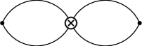
Figure 1: Perturbation theory diagram at LO

The leading contribution to the asymptotic expansion is given by the diagram shown in Fig. 1. At the leading order in QCD perturbation theory the three-point function $\Pi(p_{1},p_{2})$ of Eq. (3) completely factorizes

$$\Pi(p_{1},p_{2})=\frac{8}{3}\Pi_{\mu}(p_{1})\Pi^{\mu}(p_{2})$$ (5)

into a product of the two-point correlators $\Pi_{\mu}(p)$

$$\Pi_{\mu}(p)=p_{\mu}\Pi(p^{2})$$ (6)

$$=\int dxe^{ipx}\langle 0|TJ_{\bar{B}}(x)\bar{b}_{L}\gamma_{\mu}d_{L}(0)|0\rangle.$$

At the LO the calculation of moments is straightforward since the double spectral density is explicitly known in this approximation. Indeed, using dispersion relation for the two-point correlator

$$\Pi(p^{2})=\int_{m^{2}}^{\infty}\frac{\rho(s)ds}{s-p^{2}},$$ (7)

$$\rho(s)=\frac{3}{16\pi^{2}}m^{2}\left(1-\frac{m^{2}}{s}\right)^{2}$$

one obtains the LO double spectral density in a factorized form

$$\rho^{\rm LO}(s_{1},s_{2},q^{2})=\frac{8}{3}(p_{1}\cdot p_{2})\rho(s_{1})\rho(s_{2}).$$

Thus, all PT contributions are of the factorizable form at the leading order. First non-factorizable contributions to Eq. (4) appear at NLO. Of course, at NLO there are also the factorizable diagrams. Note that the classification of diagrams in terms of their factorizability is consistent as both classes are independently gauge and RG invariant.

Figure 2: Factorizable diagrams at NLO

Consider first the NLO factorizable contributions that are given by the product of two-point correlation functions from Eq. (6), as shown in Fig. 2. Analytical expression for such contributions can be obtained as follows. Writing $\Pi(p^{2})=\Pi_{\rm LO}(p^{2})+\Pi_{\rm NLO}(p^{2})$ one finds

$$\Pi_{\rm NLO}^{f}(p_{1},p_{2})=\frac{8}{3}(p_{1}.p_{2})(\Pi_{\rm LO}(p_{1}^{2})\Pi_{\rm NLO}(p_{2}^{2})$$

$$+\Pi_{\rm NLO}(p_{1}^{2})\Pi_{\rm LO}(p_{2}^{2})).$$

The spectral density of the correlator $\Pi_{\rm NLO}(p^{2})$ is known analytically that solves the problem of the NLO analysis in factorization. Even a NNLO analysis of factorizable diagrams is possible as several moments of two-point correlators are known analytically [32].

The NLO analysis of non-factorizable contributions within perturbation theory is the main point of my talk. The analysis amounts to the calculation of a set of three-loop diagrams (a typical diagram is presented in Fig. 3). These diagrams have been computed using the package MATAD for automatic calculation of Feynman diagrams [33]. The package is applicable only for computation of scalar integrals. the decomposition of the three-point amplitude into scalars is known [34].

Figure 3: A non-factorizable diagram at NLO

The expression for the “theoretical” moments is

$$M_{th}(i,j)=\frac{m^{6}a_{ij}}{m^{2(i+j)}}\left\{1+\frac{\alpha_{s}}{4\pi}\left(b^{f}_{ij}+b^{nf}_{ij}\right)\right\}$$ (8)

where the quantities $a_{ij}$, $b^{f}_{ij}$ and $b^{nf}_{ij}$ represent LO, NLO factorizable and NLO nonfactorizable contributions as shown in Figs. 1-3. The NLO nonfactorizable contributions $b^{nf}_{ij}$ with $i+j\leq 7$ are analytically calculated in ref. [1] for the first time. The calculation has been done with the system FORM [35] and required about 24 hours of computing time on a dual-CPU 2 GHz Intel Xeon machine. The analytical result for the lowest finite moment $M_{th}(2,2)$ reads

$$a_{22}=\frac{1}{(16\pi^{2})^{2}}\left(\frac{8}{3}\right),\quad b^{f}_{22}=\frac{40}{3}+\frac{16\pi^{2}}{9}\,,$$ (9)

$$b^{nf}_{22}\!=\!S_{2}\frac{8366187}{17500}-\!\zeta_{3}\frac{84608}{875}-\!\pi^{2}\frac{33197}{52500}-\!\frac{426319}{315000}.$$

Here $S_{2}=\frac{4}{9\sqrt{3}}{\rm Cl}_{2}\left(\frac{\pi}{3}\right)=0.2604\ldots$, $\zeta_{3}=\zeta(3)$, and $\mu^{2}=m^{2}$. Higher moments contain the same transcendental entries $S_{2}$, $\zeta_{3}$, $\pi^{2}$ with different numerical coefficients. The numerical values for the moments are $b^{nf}_{ij}$: $b^{nf}_{2(2345)}=\{0.68,1.22,1.44,1.56\}$ and $b^{nf}_{3(34)}=\{1.96,2.25\}$. The above theoretical results are used to extract the non-perturbative parameter $B_{B}$ from the sum rules analysis.

5 Results for $B_{B}$

The “phenomenological” side of the sum rules reads

$$M_{ph}(i,j)=\frac{8}{3}B_{B}\frac{f_{B}^{4}m_{B}^{2}}{m_{B}^{2(i+j)}}+\ldots$$ (10)

where the contribution of the $B$-meson is displayed explicitly. The remaining parts are the contributions due to higher resonances and the continuum which are suppressed due to the mass gap $\Delta$ in the spectrum model. A rough picture of the phenomenological spectrum is given in Fig. 4.

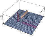
Figure 4: A model of phenomenological spectrum

For comparison we consider the factorizable approximation for both “theoretical”

$$M_{th}^{f}(i,j)=\frac{m^{6}a_{ij}}{m^{2(i+j)}}\left(1+\frac{\alpha_{s}}{4\pi}b^{f}_{ij}\right)$$ (11)

and “phenomenological” moments, which, by construction, are built from the moments of the two-point function of Eq. (6)

$$M_{ph}^{f}(i,j)=\frac{8}{3}\frac{f_{B}^{4}m_{B}^{2}}{m_{B}^{2(i+j)}}+...$$ (12)

The standard comparison of theoretical calculation with the phenomenological representation allows to extract the residue in the senior pole and, therefore $B_{B}$. Eq. (11) and Eq. (8) differ only due to non-factorizable corrections.

To find the nonfactorizable addition to $B_{B}$ from the sum rules we form ratios of the total and factorizable contributions. On the “theoretical” side one finds

$$\frac{M_{th}(i,j)}{M_{th}^{f}(i,j)}=1+\frac{\alpha_{s}}{4\pi}\frac{b^{nf}_{ij}}{1+\frac{\alpha_{s}}{4\pi}b^{f}_{ij}}\,.$$ (13)

This ratio is mass-independent. On the “phenomenological” side we have

$$\frac{M_{ph}(i,j)}{M_{ph}^{f}(i,j)}=\frac{B_{B}+R_{B}(z^{j}+z^{i})+C_{B}z^{i+j}}{1+R^{f}(z^{j}+z^{i})+C^{f}z^{i+j}}$$ (14)

where $z=m_{B}^{2}/(m_{B}^{2}+\Delta)$ is a parameter that describes the suppression of higher state contributions. $\Delta$ is a gap between the squared masses of the $B$-meson and higher states. $R_{B}$, $C_{B}$, $R^{f}$ and $C^{f}$ are parameters of the model for higher state contributions within the sum rule approach. In order to extract the non-factorizable contribution to $B_{B}$ we write $B_{B}=1+\Delta B$. Similarly, one can parameterize contributions to “phenomenological” moments due to higher $B$-meson states by writing $R_{B}=R^{f}+\Delta R$ and $C_{B}=C^{f}+\Delta C$. Clearly, $\Delta B=\Delta R=\Delta C=0$ in factorization. The final formula for the determination of $\Delta B$ reads

$$\frac{\alpha_{s}}{4\pi}b^{nf}_{ij}=\Delta B+\Delta R(z^{j-2}+z^{i-2})+\Delta Cz^{i+j-4}$$

where $\Delta R$ and $\Delta C$ are free parameters of the fit. We take $\Delta=0.4m_{B}^{2}$ for the $B$ meson two-point correlator. This corresponds to the duality interval of $1~{}{\rm GeV}$ in energy scale for the analysis based on finite energy sum rules [36]. The actual value of $\Delta B$ has been extracted using the least-square fit of all available moments. Estimating all uncertainties we finally find the NLO non-factorizable QCD corrections to $\Delta B$ due to perturbative contributions to the sum rules to be

$$\Delta B=(6\pm 1)\frac{\alpha_{s}(m)}{4\pi}.$$

We checked the stability of the sum rules which lead to a prediction of $\Delta B$. For $m_{b}=4.8~{}{\rm GeV}$ and $\alpha_{s}(m_{b})=0.2$ [37] one finds $\Delta B=0.1$.

6 Conclusion

To conclude, the $B^{0}-\bar{B}^{0}$ mixing matrix element has been evaluated in the framework of QCD sum rules for three-point functions at NLO in perturbative QCD. The effect of radiative corrections on $B_{B}$ is under complete control within pQCD and amounts to approximately $+10$% of the factorized value. The calculation can be further improved with the evaluation of higher moments. The result is sensitive to the parameter $z$ or to the magnitude of the mass gap $\Delta$ used in the parametrization of the spectrum.

References

- [1] J. G. Körner, A. I. Onishchenko, A. A. Petrov and A. A. Pivovarov, Phys. Rev. Lett. 91, 192002 (2003).
- [2] I. I. Bigi and A. I. Sanda, Cambridge Monogr. Part. Phys. Nucl. Phys. Cosmol. 9, 1 (2000).
- [3] A. D. Sakharov, Pisma Zh. Eksp. Teor. Fiz. 5, 32 (1967)
- [4] A. A. Petrov, arXiv:hep-ph/0207212.
- [5] G. Buchalla, A. J. Buras and M. Lautenbacher, Rev. Mod. Phys. 68, 1125 (1996).
-
[6]
A. Ali and D. London,
arXiv:hep-ph/0002167. - [7] B. Aubert et al. [BABAR Collaboration], Phys. Rev. D 66, 032003 (2002).
- [8] B. Aubert et al. [BABAR Collaboration], Phys. Rev. Lett. 89, 201802 (2002).
- [9] K. Abe et al. [Belle Collaboration], Phys. Rev. Lett. 86, 3228 (2001).
- [10] A. Abashian et al. [BELLE Collaboration], Phys. Rev. Lett. 86, 2509 (2001).
- [11] K. Hagiwara et al., Phys. Rev. D 66, 010001 (2002).
-
[12]
F. J. Gilman and M. B. Wise, Phys. Rev.
D 27, 1128 (1983); A. J. Buras, arXiv:hep-ph/9806471. - [13] A. J. Buras, M. Jamin and P. H. Weisz, Nucl. Phys. B 347, 491 (1990); J. Urban et al., Nucl. Phys. B 523, 40 (1998).
- [14] T. Inami and C. S. Lim, Prog. Theor. Phys. 65, 297 (1981).
- [15] M. Gaillard and B. Lee, Phys. Rev. D 10, 897 (1974).
- [16] J. Bijnens, H. Sonoda and M. B. Wise, Phys. Rev. Lett. 53, 2367 (1984); W. A. Bardeen, A. J. Buras and J. M. Gerard, Phys. Lett. B 211, 343 (1988).
-
[17]
K. G. Chetyrkin et al.,
Phys. Lett. B 174,
104 (1986); L. J. Reinders and S. Yazaki,
Nucl. Phys. B 288, 789 (1987); K. G. Chetyrkin and A. A. Pivovarov, Nuovo Cim. A 100, 899 (1988). - [18] A. A. Ovchinnikov and A. A. Pivovarov, Phys. Lett. B 207, 333 (1988); A. A. Pivovarov, Nucl. Phys. Proc. Suppl. B 23, 419 (1991); Pisma v ZETF 55, 8 (1992), arXiv:hep-ph/9606482.
-
[19]
L. J. Reinders and S. Yazaki,
Phys. Lett. B
212, 245 (1988). - [20] A. Pich, Phys. Lett. B 206, 322 (1988); S. Narison and A. A. Pivovarov, Phys. Lett. B 327, 341 (1994).
- [21] D. Melikhov and N. Nikitin, Phys. Lett. B 494, 229 (2000).
- [22] A. A. Pivovarov, Phys. Lett. B 236, 214 (1990), Nucl. Phys. B 396, 119 (1993), Yad. Fiz. 59, 930 (1996).
- [23] D. Becirevic et al., Phys. Lett. B 487, 74 (2000); D. Becirevic et al., Nucl. Phys. B 618, 241 (2001); M. Lusignoli, G. Martinelli and A. Morelli, Phys. Lett. B 231, 147 (1989); M. Lusignoli et al., Nucl. Phys. B 369, 139 (1992); C. T. Sachrajda, Nucl. Instrum. Meth. A 462, 23 (2001); J. M. Flynn and C. T. Sachrajda, Adv. Ser. Direct. High Energy Phys. 15, 402 (1998).
- [24] A. Hiorth and J. O. Eeg, Eur. Phys. J. C 30, 006 (2003).
- [25] A. A. Pivovarov, Int. J. Mod. Phys. A 10, 3125 (1995).
- [26] M. A. Shifman, A. I. Vainshtein and V. I. Zakharov, Nucl. Phys. B 147, 448 (1979).
-
[27]
N. V. Krasnikov, A. A. Pivovarov and
A. N. Tavkhelidze, Pisma Zh. Eksp. Teor. Fiz. 36, 272 (1982), Z. Phys. C 19, 301 (1983); A. A. Pivovarov, Z. Phys. C 53, 461 (1992). - [28] C. Becchi, S. Narison, E. de Rafael and F. J. Yndurain, Z. Phys. C 8, 335 (1981); S. Narison and E. de Rafael, Phys. Lett. B 103, 57 (1981).
- [29] J. Gasser and H. Leutwyler, Phys. Rept. 87, 77 (1982).
-
[30]
A. L. Kataev, N. V. Krasnikov and
A. A. Pivovarov, Phys. Lett. B 123, 93 (1983), Nuovo Cim. A 76, 723 (1983);
K. G. Chetyrkin, J. H. Kühn and A. A. Pivovarov, Nucl. Phys. B 533, 473 (1998);
J. G. Körner, F. Krajewski and A. A. Pivovarov, Eur. Phys. J. C 20, 259 (2001), Eur. Phys. J. C 14, 123 (2000). - [31] K. Hagiwara, S. Narison and D. Nomura, Phys. Lett. B 540, 233 (2002)
- [32] K. G. Chetyrkin, M. Steinhauser, arXiv:hep-ph/0108017.
- [33] M. Steinhauser, Comput. Phys. Commun. 134, 335 (2001).
- [34] A. I. Davydychev and J. B. Tausk, Nucl. Phys. B 465, 507 (1996).
- [35] J. A. Vermaseren, arXiv:math-ph/0010025.
- [36] N. V. Krasnikov and A. A. Pivovarov, Phys. Lett. B 112, 397 (1982); A. A. Pivovarov, Yad. Fiz. 62, 2077 (1999)
- [37] J. H. Kühn, A. A. Penin and A. A. Pivovarov, Nucl. Phys. B 534, 356 (1998); A. A. Penin and A. A. Pivovarov, Phys. Lett. B 435, 413 (1998), Nucl. Phys. B 549, 217 (1999).