Morphology and Characteristics of Radio Pulsars

Abstract

This review describes the observational properties of radio pulsars, fast rotating neutron stars, emitting radio waves. After the introduction we give a list of milestones in pulsar research. The following chapters concentrate on pulsar morphology: the characteristic pulsar parameters such as pulse shape, pulsar spectrum, polarization and time dependence. We give information on the evolution of pulsars with frequency since this has a direct connection with the emission heights, as postulated in the radius to frequency mapping (RFM) concept. We deal successively with the properties of normal (slow) pulsars and of millisecond (fast - recycled) pulsars. The final chapters give the distribution characteristics of the presently catalogued 1300 objects.

1 Introduction

The first publication Hewish68 announcing the discovery of a new class of objects, soon to be known as pulsars Manchester77a Lyne90a , appeared in the literature almost exactly 35 years ago. Since then, large strides toward the understanding of pulsars and their radiation have been made. We know that they are fast rotating

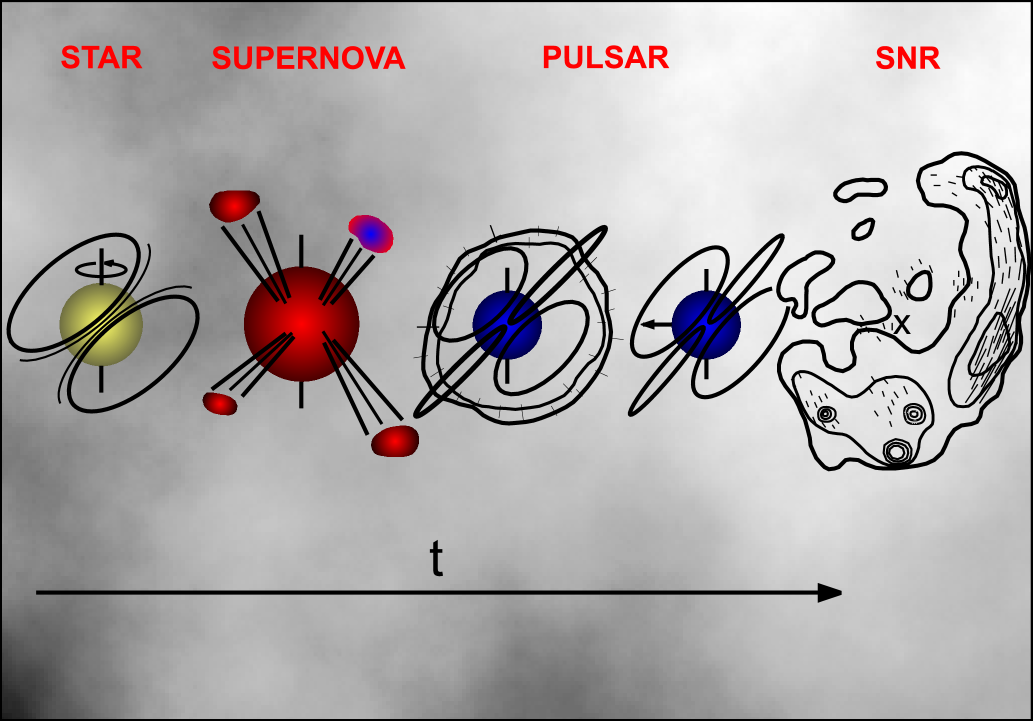
Figure 1: Scenario of the birth and evolution of pulsars

neutron stars Baade34a Baade34b Nollert88 with masses of the order of 1 M_⊙ Pandharipande76 Datta83 Thorsett93 Kalogera96 Callanan98 Thorsett99 Srinivasan02 Haensel02 Jonker03 and strong magnetic field (between $10^{9}$ and $10^{14}$ Gauss Flowers77 Beskin86 Romani90 Michel91 Arons93 Zhang00 . They are probably born during a Supernova Type II explosion of a (massive) late-type star (Fig. 1).

Pulsars emit highly accurate periodic signals (mostly in radio waves), beamed in a cone of radiation, centred around their magnetic axis. These signals reveal the period of rotation of the neutron star, which radiates, like a light-house, once per revolution. The lighthouse effect is caused by the dipolar magnetic field not being aligned with the rotation axis of the neutron star. As a consequence of the magnetic field, pulsar radiation is highly polarized. Their period of rotation (P) varies between 1.557 ms (642 Hz) Backer82 and 8.5 s (0.12 Hz) Young99 . As pulsars rotate, they loose energy and their rate of rotation decreases. This period derivative ($\dot{P}$) is an important observational parameter. In 1975 a pulsar in a binary system was discovered Hulse75 . Slow rotating pulsars, with rotation period P $\geq$ 20 ms and $\dot{P}>10^{-18}$ are considered to be normal pulsars. Pulsars with P $<$ 20 ms and $\dot{P}\leq 10^{-18}$ are called millisecond or recycled pulsars. A full list of 1300 pulsars Manchester03 is available at http://www.atnf.csiro.au/research/pulsar/psrcat/.

The period of rotation of normal pulsars increases with time, an observational fact, discovered during the very early history of pulsars Richards69 and led to the rejection of suggestions that the periodic signals could be due to the orbital period of binary stars. The orbital period of an isolated binary system decreases as it looses energy, whereas the period of a rotating body increases as it looses energy. Millisecond pulsars are considered to be recycled pulsars, spun up by mass transfer (accretion) from a binary companion Alpar82 . In the early history of pulsars, models involving pulsations of white dwarfs and neutron stars were also proposed and quickly rejected.

Table 1: Pulsar milestones

Date	Milestone	Reference
1932, Feb	The discovery of neutron	Chadwick32a , Chadwick32b
1934, 1967	Neutron stars are predicted	Baade34a , Pacini67
1939	Neutron stars Equation of State	Oppenheimer39
1967, Nov 28	The discovery of pulsars	Hewish68
1967, Nov 28–1968, Mar 03	“Pulsar” designation	Bell79
1968, Mar 15	First published “Pulsar” designation	Telegraph68 ,Time68
1968	Discovery of the Vela pulsar	Large68a
1968	Discovery of the Crab pulsar	Staelin68 ,Comella69
1968, Feb 24	Dispersion measure measured	Davies68
1968, Apr 01	First polarimetric observation	Lyne68a
1968, Apr 03	Faraday Rotation measured	Smith68
1968	Gravitational emission proposed	Weber68
1968	Lighthouse model proposed	Gold68
1968, Nov	Galactic distribution established	Large68b
1969	Post-detection of pulsar X-rays	Fishman69a
1969	Post-detection of pulsar $\gamma$-rays	Fishman69b
1969	Scintillation explained	Rickett69
1969	Rotating Vector Model proposed	Rad69a
1969	Observations of pulsar glitches	Rad69b
1969, Aug	First emission process proposed	Goldreich69
1974, Jul 02	Discovery of binary pulsars	Hulse75
1975	First complete theory attempted	Ruderman75
1982	Discovery of millisecond pulsars	Backer82
1991, S̃ep 15	Detection of extrasolar planets	Wolszczan92
1992, Oct 19	Detection at mm-wavelengths	Wielebinski93
1998	Discovery of magnetars	Kouveliotou98
1998, Nov 05	Discovery of the 1000th pulsar	csiro98

The discovery of the Vela pulsar (PSR 0833-45 – see Table 1) led to the suggestion of pulsar – supernova association. This suggestion was corroborated by the discovery of a pulsar (PSR 0531+21) in the heart of the Crab supernova remnant with a period of 33 milliseconds (see Table 1), which led to the unequivocal association of (radio) pulsars with rotating neutron stars Gold68 . Subsequent polarimetric observations led to the establishment of the “Rotating Vector Model” Rad69a . Soon after its discovery, the Crab pulsar was post-detected in earlier (1967, Jun 04) archived X-ray data Fishman69a and soft $\gamma$-ray data Fishman69b . To date (excluding non-pulsed detections of neutron stars) 5 normal pulsars have been detected in the optical, 17 normal and 6 millisecond pulsars in X-rays and 7 normal pulsars in $\gamma$-rays (up to $10^{25}$ Hz, covering, thus, the largest frequency range of all known compact species emitting intense radiation in the Universe) (updated information from Becker02 - W. Becker, private communication). The first (and fastest, up to now) millisecond pulsar, PSR B1937+214 was discovered in 1982 (Backer82 . Ten years later the first planetary system (two planets orbiting PSR B1257+12), outside the solar system, was discovered (Wolszczan92 ).

The discovery of millisecond and binary pulsars (see Table 1) gave new insight in pulsar research. It was soon realized that the extremely fast rotation of millisecond pulsars could only be explained by transfer of angular momentum from companion stars. The notion of recycling of old and exhausted neutron stars became popular. On the other hand binary pulsars were used to check the effects of General Relativity, which successfully survived the new tests. For these particular discoveries the Nobel Price in Physics (see http://www.nobel.se/physics/laureates/) was twice awarded to pulsar researchers: In 1974 it was awarded to Antony Hewish for the discovery of the first pulsar, PRS B1919+21, and in 1993 to Russell A. Hulse and Joseph H. Taylor for the discovery and subsequent work on the physics of the binary pulsar PSR B1913+16. Recently the discovery of a double pulsar system, PSR J0737-3039B (spin period 2.7 sec), PSR J0737-3039A (spin period 22 msec) in a 2.4 hr eccentric orbit was announced Lyne04 . This system will, certainly play a very important role in deciphering the pulsar riddle and in testing physical theories.

Meanwhile, a large number of strange and unexpected properties of pulsar emission were observed. Drifting subpulses, mode changing and nulling were among the first such properties to be studiedRankin86a . Extremely narrow pulses Hankins71 Kramer02 Hankins03 were soon to become an important tool for theoretical investigations and $90{\hbox{${}^{\circ}$}}$ polarization jumps (orthogonal modes) imposed restrictions to the existing models. In addition, period glitches were observed, during which the pulsar period decreased by a large amount and then, within a few days, it increased again to its previous value. Glitch properties are used to study the physical structure of neutron stars.

2 Pulsar Milestones

Before proceeding with the description of the characteristics of pulsar emission, it is worth looking back and paying tribute to the main discoveries concerning pulsars. Table 1, summarises the most important steps in pulsar research, both in observation and theory.

It is not always easy to unearth a “first” date or a “first” publication. For example, J. Bell-Burnell has communicated to us her personal view Telegraph68 and we have found a report in a March 1968 issue of the Time magazine Time68 referring to the first use of the word pulsar. Nevertheless, we believe that still earlier references to the “pulsar” notation may have escaped our search. The list can be expanded to include several other “firsts”. However, we decided to restrict its size to what we consider to be the most important ones.

3 Morphology

Pulsars present to the observer a most complicated set of time variable phenomena. On the one hand, their period of rotation, P, varies from 1.5 millisecond up to 8.5 seconds from object to object. On the other, this period increases regularly with time, as the pulsar looses gravitational energy and slows down. The deceleration is

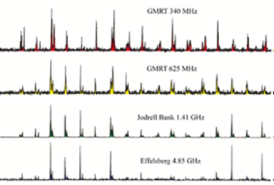
Figure 2: A sequence of 17 single pulses observed simultaneously at 4 frequencies, plotted one after the other. Courtesy of A. Karastergiou

expressed quantitatively by the measured $\dot{P}$. The youngest (normal) pulsars exhibit usually the largest deceleration and thus they demonstrate the largest $\dot{P}$. Quite to the opposite, millisecond pulsars have very low $\dot{P}$ and are interpreted to be recycled objects, slow, normal pulsars that have been sped up by accretion from a binary counterpart. The deceleration process is not always constant. Some pulsars are known to exhibit glitches, sudden acceleration to higher periods, which are interpreted to be due to crust related “starquakes”.

Taking into account single pulse intensities and their duration, extremely high brightness temperatures (of the order of $10^{29}$ K) are calculated, especially for their low frequency emission. This constrains their radio emission to be coherent (see also Lesch98 and references therein). The intensity of single pulses show enormous intrinsic variations. The situation is even further complicated by the fact that interstellar scintillation introduces an additional fluctuating effect, in particular at lower radio frequencies. However with enough repeated observations the average emitted pulsar flux density can be determined. The addition of a sequence of single pulses leads quickly (usually, after a few hundred pulses) to a stable pulse shape, a signature of the geometry of lighthouse emission mechanism. The pulse shape is a firm characteristic of a pulsar, having anything from one up to nine sub-pulse components.

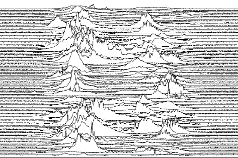
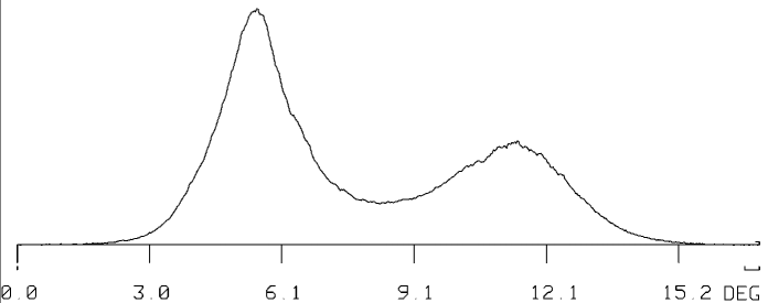
Figure 3: (Top): A sequence of 100 single pulses from PSR 1133+16 plotted underneath each other (Noise wings are suppressed). (Bottom): By adding the above single pulses, we get the Integrated profile

Within the sub-pulse structure a number of phenomena has been observed. Sub-pulse drifting (see above) reveals the emitting beam structure. In addition, the existence of very narrow pulsar micro- and nano-structure Ferg78 Hankins03 , that are the signs of individual emission regions, has been confirmed. Pulsar radiation is highly polarized in a most complicated way. At low radio frequencies some pulsars are almost 100% linearly polarized. Others have very high and variable circular polarization. The development of polarization with frequency is radically different from all other radio sources. The polarization may be high at low frequencies while dropping rapidly to zero at high frequencies. Possibly this is a hint for a coherent (low frequencies) – incoherent (high frequencies) emission mechanism, an effect corroborated by high frequency pulsar spectra Kramer96 .

3.1 Displaying pulses

Pulsars are immediately recognised from the periodic nature of their radiation. Pulse sequences (Fig. 2) can be depicted in a much more compact and informative way if their period is accurately known. Then, instead of showing the pulses one-after-the-other, they can be displayed one-underneath-the-other. Thus, many more pulses can be conveniently accommodated in a single graph. By ignoring the unpulsed noise either side of the pulses, high time resolution single pulses are readily displayed (Fig. 3 - top). It is evident from Figures 2 and 3 that individual, single pulses vary greatly in intensity. Most of these variations are intrinsic. Some are due to interstellar scintillation. However, if a large number of single pulses are added together, a very stable profile is obtained (Fig. 3 - bottom). For most pulsars, this integrated profile characterizes uniquely a pulsar at a particular frequency. The stability of pulsar integrated profiles has been thoroughly investigated for a large sample of normal pulsars Helfand75 and some millisecond pulsars Kaspi93 .

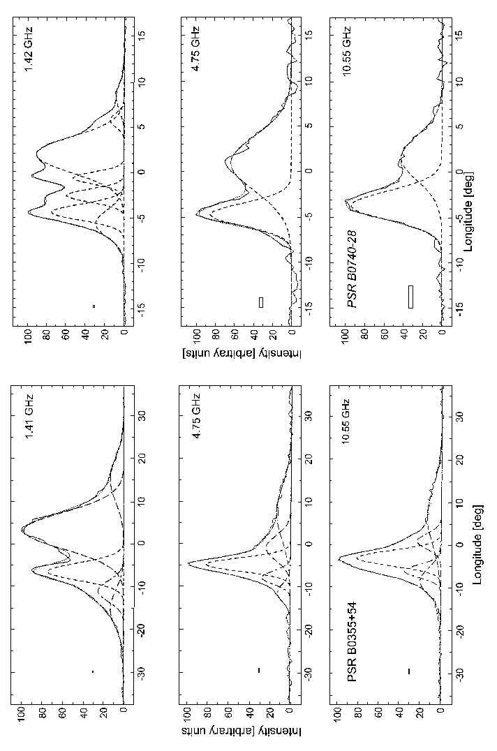
Figure 4: Time-aligned profiles at three frequencies, with gauss-fitted components. Radius to Frequency Mapping (RFM) is obvious in this Figure. Left panel: PSR B0355+54. Right panel: PSR B0740-28.

3.2 Integrated Pulses

In the integrated pulsar profiles distinct components can be identified Seiradakis95 Kijak98 . They are thought to represent coherent physical regions in the magnetosphere of the star. Therefore their properties are of extreme importance for understanding the emission mechanism of pulsars. These components are often blended and their shape and longitudinal location within the pulsar profile is difficult to establish. A large collection of pulse profiles can be found in the European Pulsar Network data archive at www.mpifr-bonn.mpd.de/div/pulsar/data/. Although there are no rigorous theoretical arguments, usually they can be fitted with gaussian curves, the parameters of which are easily obtained. Experience has shown that pulsar profiles can indeed be reconstructed by a sum of individual gaussian components. This method usually involves some assumptions which can be minimized by reducing the number of degrees of freedom of the gauss–fitting procedure Kramer94a Kramer94b . Some gauss–fitted components are shown in Fig. 4.

Figure 5: Integrated profiles of pulsars at 1.41 GHz Seiradakis95

Figure 6: Integrated profiles of pulsars at 10.7 GHz Seiradakis95

3.2.1 Normal Pulsars (P $\geq$ 20 ms)

Pulse profiles come in a variety of shapes (Fig. 5, 6). In most cases they can be represented by a smooth curve with a single (almost gaussian) component or with two or more components. Soon after the discovery of pulsars, it was realised that their integrated profiles exhibit important morphological differences. In order to explain double profiles, the hollow cone model was proposed in the early seventies Komesaroff70 Backer76 Oster76 . Triple profiles were explained by the introduction of a central pencil beam and five-component profiles were interpreted by assuming a more complicated beam, comprising of a central beam surrounded by an inner and an outer cone Rankin83a Rankin83b Rankin93a Rankin93b . The number of cones that can be accommodated within the narrow polar cap region, whose radius is bound by the last open magnetic field lines cannot be very large. It is interesting that pulsars exhibiting a single core component, seem to occupy a distinct region in the P$\dot{P}$ diagram Gil99 (Fig. 21).

Figure 7: Integrated profiles of millisecond pulsars at 1.41 GHz. Effelsberg observations, M. Kramer et al.

On the other hand a patchy beam model was proposed Lyne88 , according to which pulsar beams are patchy, with components randomly located within the last open magnetic field lines. This model is based on the fact that single pulses vary in intensity and often they seem to be missing altogether. There have been several attempts to explain the pulsar beam shapes using both theoretical and geometrical arguments Gil93 Manchester95 Gil97 Mitra99 . However, there are still many uncertainties due to the erratic behaviour of pulsar emission and the lack of an accepted model for pulsar radiation.

3.2.2 Millisecond (Recycled) Pulsars (P $<$ 20 ms)

The first millisecond pulsars to be discovered exhibited rather simple profiles. Nowadays about 100 millisecond pulsars have been detected, many of which have complex integrated profiles Kramer99 , not dissimilar to the profiles of normal pulsars (Fig. 7). One difference is that millisecond pulsars tend to have wider profiles than normal pulsars.

3.2.3 Radius to Frequency Mapping

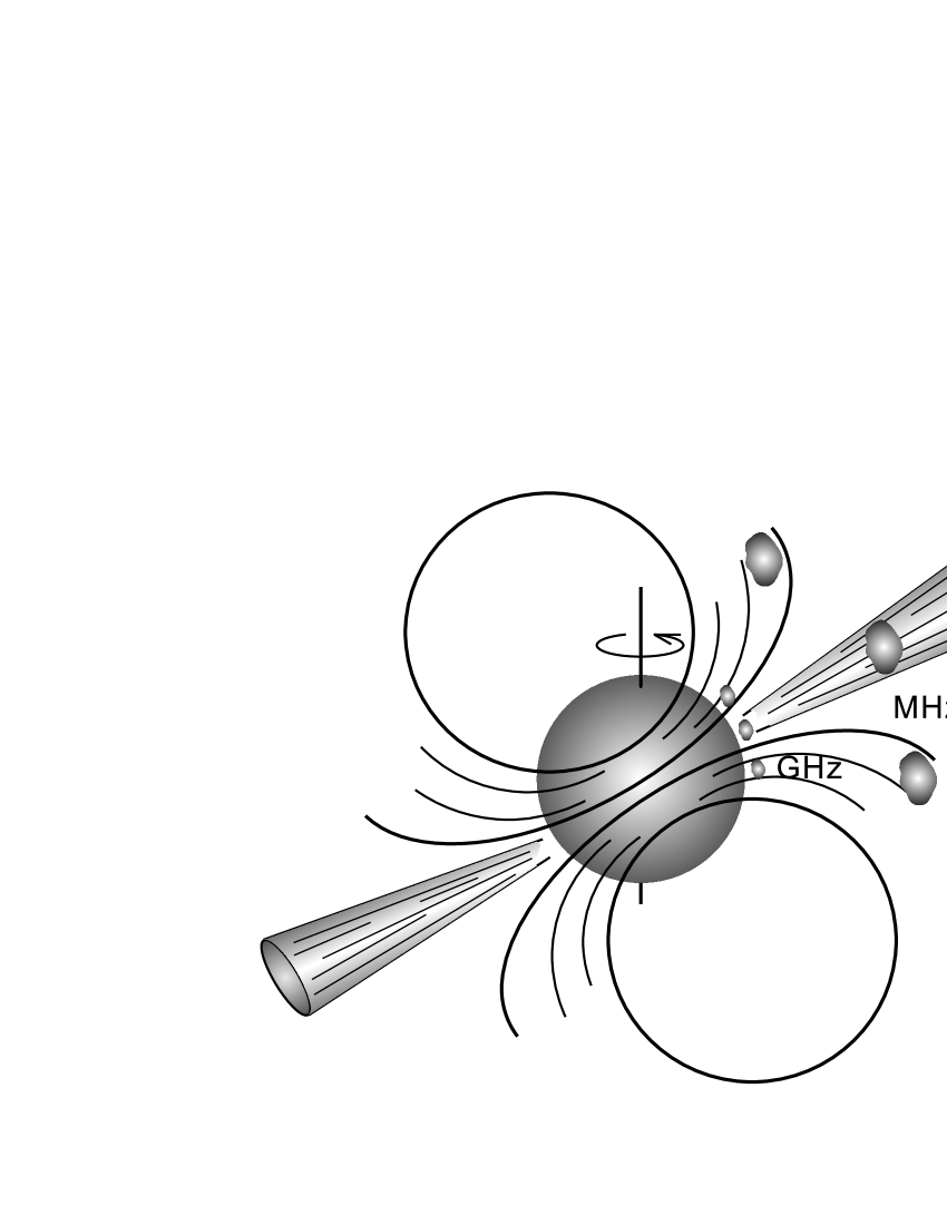
Figure 8: Radius to Frequency Mapping (RFM). High frequencies are emitted close to the surface of the star. Low frequencies are emitted higher up, where the cone of emission is wider

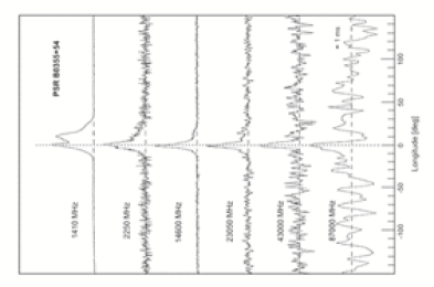
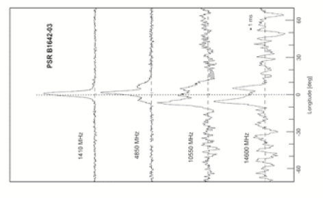
Figure 9: The development of pulsar integrated profiles with frequency. Note that new components can appear both at high and low frequencies. Courtesy M. Kramer

The frequency development of pulse shapes has led to the concept of a Radius to Frequency Mapping (RFM - Fig. 8), according to which, higher radio frequencies are emitted in the lower reaches of the pulsar magnetosphere (closer to the surface of the star). In order to investigate the RFM concept, time-aligned pulse shapes are needed, that require accurate pulsar timing. Following the standard pulsar model Ruderman75 the integrated pulse width is expected to decrease monotonically with frequency (RFM effect). This effect was implicit in earlier work Sieber75 and has been extensively investigated ever since Cordes78 AvH97b . Multi frequency observations of pulsars have confirmed the narrowing of pulse profiles with frequency Kuzmin98 Kramer99 . The effect is adequately demonstrated for both normal and millisecond pulsars in Figures 4, 9 and 10.

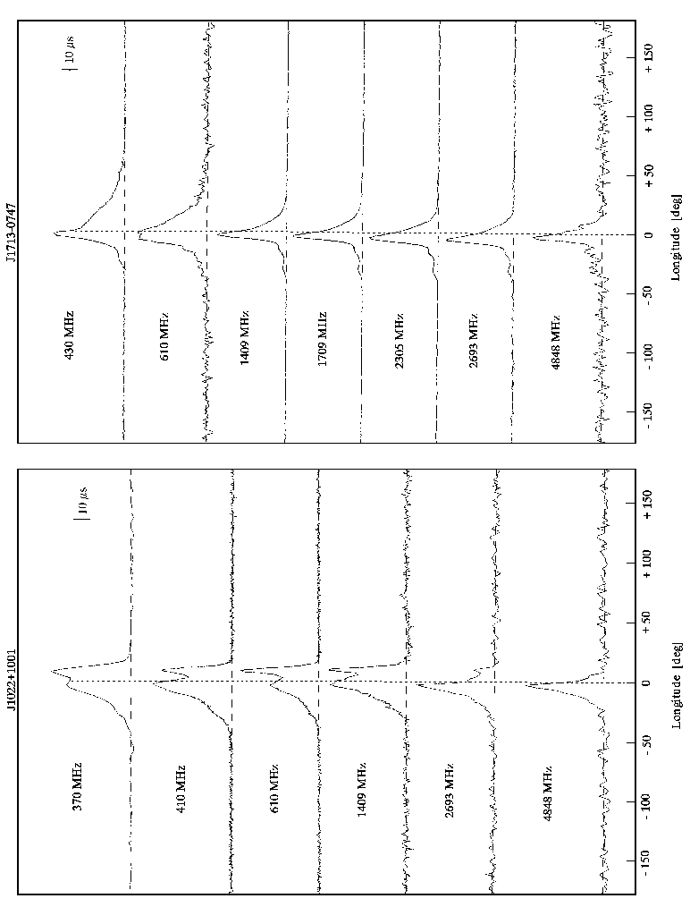
Figure 10: The development of millisecond pulsars integrated profiles with frequency. Adapted from Kramer99

3.2.4 The Crab pulsar from radio frequencies to $\gamma$-rays

The Crab pulsar (PSR B0531+21) is probably, the best studied pulsar. Soon after its discovery, archival searches led to post detection of pulsed emission at X-rays and $\gamma$-rays Fishman69a , Fishman69b . Its “main-pulse – interpulse” integrated profile is unmistakably evident throughout the electromagnetic spectrum (Fig. 11). However, carefully time-aligned profiles Moffett96 reveal slight, but significant, displacement of its high frequency components from its lower (radio) components. This has been interpreted as evidence of two different mechanisms of emission, with the high frequency emission (optical, X-rays, $\gamma$-rays) originating in a region close to the light cylinder. Furthermore, recent investigations Moffett96 Karastergiou03c have revealed that between 4.7 GHz and 8.4 GHz extra components appear in its integrated profile (Fig. 11). These components impose additional difficulties in the investigation of the emission mechanism of this interesting object.

Figure 11: The integrated profile of the Crab pulsar from low frequency radio waves to soft gamma-rays. Note the absence of the main pulse and the peculiar extra components between 4.7 and 8.4 GHz. Courtesy T.H. Hankins

3.3 Single Pulses

Investigations of single pulses is of utmost importance, showing the variability and spatial structure of the pulsar emission process. Already in the discovery paper Hewish68 and other early papers Davies68 Large68b Craft68 Ekers68 Robinson68 single pulses at low frequencies were studied. Single pulses show a variety of sharp emission structures from millisecond through microsecond down to nanosecond range Craft68 Hankins71 Lange98 Hankins03 . Early two-frequency simultaneous observations suggested that the emission is inherently broad-band Bartel78a , i.e. emission is correlated over a wide frequency range. Later observations Boriakoff81a Bartel81 Davies84 Kardashev86 were made for total intensity only and at most for two simultaneous frequencies. Most of these investigations were then used to determine the bandwidth of the emission. More recently, using many radio telescopes at different frequencies, simultaneously, at up to five frequencies Kramer03 have investigated the single pulse characteristics in detail (see also Fig. 2).

3.4 Millistructure, Microstructure, Nanostructure

The fact that very short time structures are present in single pulses was noted from the very beginning Hewish68 leading to a stringent requirement for theories attempting to explain the origin of pulsar emission. First observation of pulsar millistructure was made soon after their discovery Craft68 . The limitation was due to signal to noise in the narrow band receiver needed to show such short time structures. A few years later a de-dispersion technique at the frequency of 115.5 MHz revealed time structures as short as 8 $\mu$s in PSR 0950+08 Hankins71 . Direct observations at 1420 MHz on PSR 1133+16 Ferg76 resolved structures with time scale of   14 $\mu$s. The microstructure was found to be broad-band Rickett75 Boriakoff81a . Periodic structures were observed that seem to be also correlated across a wide frequency range Bor81b . More recently Lange98 microstructure investigations were extended up to 4.85 GHz, showing that many pulsar have this emission signature. This result was confirmed in the studies of the Vela pulsar which shows microstructure Kramer02 in most of the pulses. Most recently the time structure studies were taken in to the nanosecond range with observations of giant pulses from the Crab pulsar Hankins03 . Their best time resolution was in fact 2 nanoseconds. This latest observation suggests that the plasma responsible for such emission must be of the order of one meter in size. If the emission is isotropic, these nanosecond pulses must be the brightest transient source in the radio sky.

4 Flux densities

The flux density of a radio source and its frequency evolution (its spectrum) are basic information that relate to the emission mechanism. However, one of the problems with flux densities is that pulsars vary on various time scales: (a) due to inherent variations Stinebring00 or (b) due to scintillations Malofeev00 or (c) due to scattering Lohmer02 .

For low frequency radio waves of the Milky Way the spectrum of the radio emission could be explained only by the non-thermal (synchrotron) emission process. From the very beginning of pulsar observations it was clear that the spectra of pulsars were very different from all other known radio sources Lyne68b Robinson68 . Instead of values of $\alpha\sim$ – 0.8 ( S = $\nu^{\alpha}$), as in cosmic radio sources, the observed spectral index of pulsars was $\alpha\sim$ – 1.5 on average. The spectral index at the highest frequencies was for some objects much higher than this average value. At lower radio frequencies a spectral turn-over was observed. It was known in the earliest papers that pulsars were very weak at higher frequencies posing in fact a great instrumental challenge to study these objects at cm wavelengths.

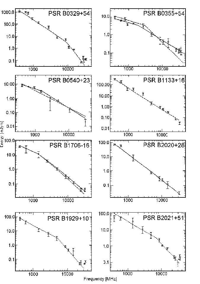
Figure 12: Spectra of pulsars detected at 9 mm. Wielebinski02

4.1 Normal Pulsars (P $\geq$ 20 ms)

The first spectra of pulsars, using flux density values at three (plus an upper limit at 1.4 GHz) frequencies, were obtained in 1968 Lyne68b . Earlier observations Robinson68 , published slightly later, were obtained at five frequencies, four of them simultaneously, giving an average spectrum and spectra of individual (single) pulses of PSR1919+21. The average spectrum was extended to 2.7 GHz and suggested a spectral break with an index of $\alpha\sim$ – 3.0 above 1.4 GHz. The data collection to determine flux densities of a larger sample of pulsars took many years to complete. While numerous observatories (Arecibo, Jodrell Bank, Green Bank, Parkes) made observations at frequencies of 1.4 GHz and below only the Goldstone facility detected pulsars at 13cm Ekers68 . Observations of the low frequency extension of pulsar spectra were carried out in the Soviet Union Brezgunov71 Bruck73 Malofeev00 at frequencies as low as 10 MHz. Three pulsars were detected at 8.1 GHz Huguenin71 . The suggested existence of a spectral break at high radio frequencies Robinson68 was later confirmed Backer72 .

A major step forward in the measurement of pulsar flux densities at high radio frequencies and hence of pulsar spectra was made by the commissioning of the 100-m Effelsberg radio telescope. Immediately, six pulsars were detected at 2.8 cm wavelength Wielebinski72 . This telescope continued to set records of the highest frequencies at which pulsars could be studied by reporting detections at 22.7 GHz Bartel77 Bartel78b and finally in the mm-wavelengths Wielebinski93 Kramer97 . A detection of the pulsar PSR 0355+54 at 3 mm wavelength has also been achieved with the Pico Veleta telescope Morris97 .

The early measurements of flux density of the strongest pulsars had to give way to studies of larger samples, if possible with a wide frequency flux density coverage. An early compendium of pulsar spectra was given for 27 pulsars Sieber73 . Further multi-frequency spectra have been presented Backer74 Sieber75 . In both of these papers the spectral breaks of some pulsars at high frequencies were confirmed and in the latter work the frequency evolution of the pulse width was noticed (this eventually led to the Radius-to-Frequency Mapping concept). Low radio frequency observations Malofeev80 confirmed the cut-off in pulsar spectra for a number of objects.

Subsequently, the flux density of a larger sample of pulsars was measured at several frequencies Seiradakis95 Lorimer95 Kijak98 and spectra of pulsars were derived Malofeev94 Toscano98 Maron00 (Fig. 12). From all these publications the conclusion was that the average spectral index is $<\alpha>$ = –18. From our gauss fitted distribution (see below) we have found a similar value, $<\alpha>$ = –1.75. It is obvious from Figure 26, that the distribution is fairly wide. Some 10% of all pulsars require a two power law fit in the high frequency range. A small number of pulsars have been recognized with almost flat spectrum ($\alpha>$ –1.0) Maron00 . In addition pulsar spectra seem to follow the power law down to low frequencies (a few 10s of MHz) with a few exceptions, where a turn-down is observed.

4.2 Millisecond Pulsars (P $<$ 20 ms)

Millisecond pulsars were discovered in 1982 Backer82 as a result of a search in the direction of radio sources with very steep spectra. The flux density of these objects is very low. This, combined with the effects of interstellar broadening, rendered their detection difficult. Early studies of millisecond pulsars Erickson85 Foster91 suggested that these objects have spectra steeper than slow pulsars. Recently high frequency observations of millisecond pulsars were also made Kijak97 Maron04 in spite of their low flux densities. The spectra of 20 objects were studied at lower radio frequencies in a survey of 280 pulsars Lorimer95 in the northern hemisphere. Several southern millisecond pulsars were also studied Toscano98 in a narrow frequency range. A major study of millisecond pulsars Kramer98 Xilouris98 Kramer99 showed that once a volume-limited sample is considered, many of the characteristics of slow and fast pulsars (spectrum, pulse shapes, number of sub-pulse components, polarization) are the same. The one distinct difference is found in the luminosity. Slow pulsars are some 10 times more luminous than millisecond pulsars. An investigation of the low frequency turn-over of millisecond pulsars Kuzmin01 Malofeev03 revealed that the morphology of millisecond pulsars is very similar to that of normal pulsars but with lower luminosity.

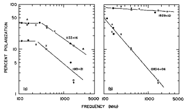
Figure 13: Early pulsar polarization Manchester71a showing the frequency dependence

5 Polarisation

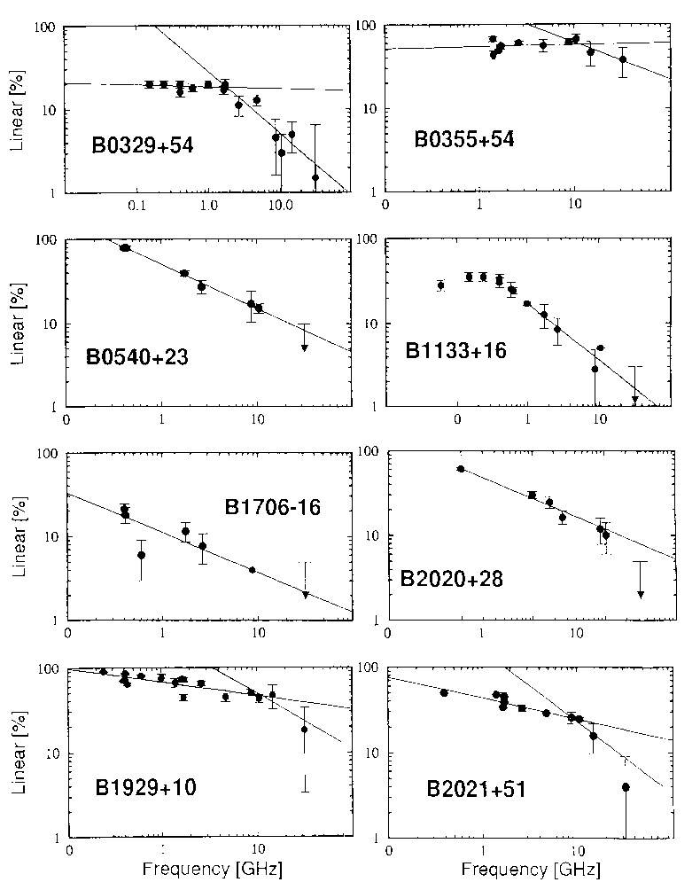
Figure 14: Polarisation development with frequency of the integrated pulses of normal pulsars for the sample of pulsars shown in Fig. 12 Wielebinski02

Soon after the discovery of pulsars Hewish68 their linear polarization was also discovered Lyne68a using the Jodrell Bank Mark I radio telescope. Variations of the intensity from pulse to pulse were detected from orthogonal dipoles connected to a high speed recorder. The linear polarization was found to be surprisingly high even at lower (150 MHz; 408 MHz) radio frequencies. Soon it was realized that considerable circular polarization was also present in pulsar emission Craft68 Clark69 . The early observations with the Parkes telescope Rad69a of the pulsar PSR B0833-45 showed a very high degree of linear polarization of the integrated pulse (in fact nearly 100%) and gave arguments for a (magnetized) rotating vector model for pulsars. The observations that followed, e.g. Ekers69 Morris70 , showed that the phase-drift of the linear polarization is a common feature in pulsars and, hence, gave support for the rotational model.

5.1 Integrated Pulses

After these early observations a number of observers embarked on determining the detailed polarization characteristics of larger samples of pulsars. In all these studies all four Stokes parameters were observed since pulsars unlike extra-galactic sources showed high degree of linear and circular polarization.

5.1.1 Normal Pulsars (P $\geq$ 20 ms)

In 1971 the results of observations of 21 pulsars, at the frequencies of 410 and 1665 MHz were

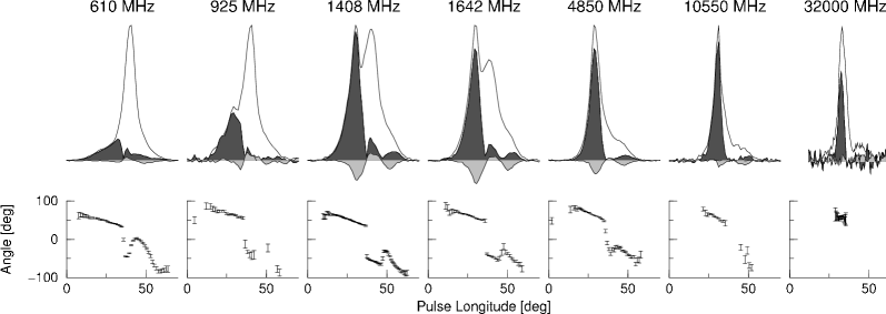
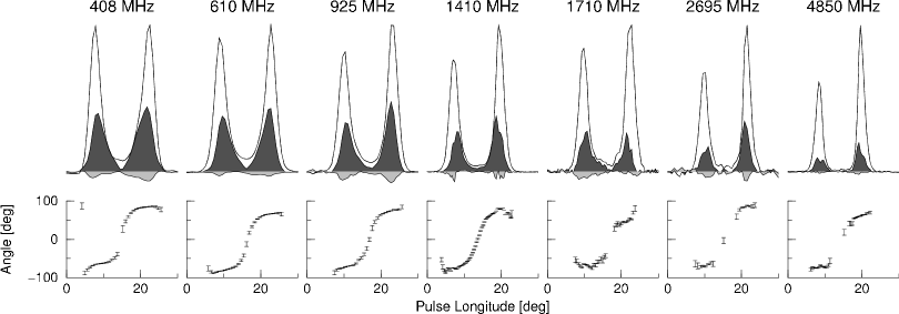
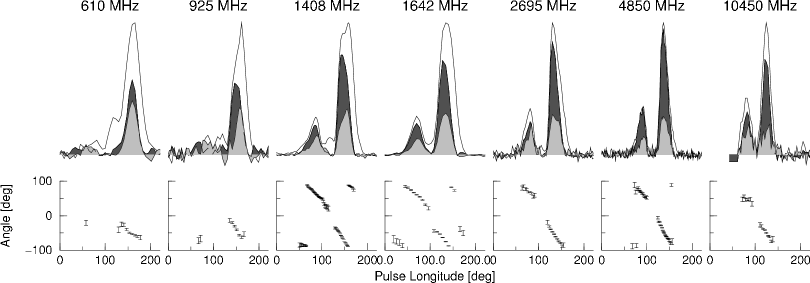
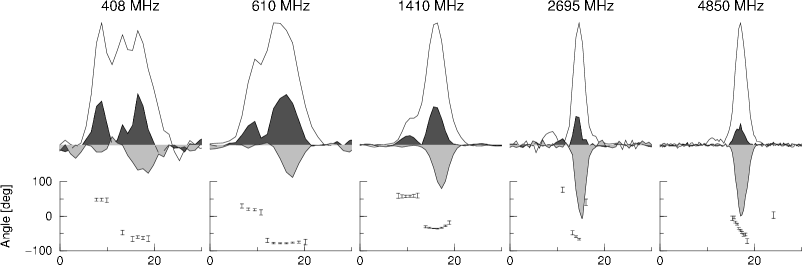
Figure 15: Characteristic polarization behaviour of pulsars. The dark-shaded area represents linearly polarized power and the light-shaded area circularly polarized power. (a): PSR B0355+54. (b): PSR 0525+21. (c): PSR B1800-21. (d): PSR 0144+59. From AvH99

published Manchester71a (Fig. 13). Numerous studies of the Crab pulsar in polarization have also been made Campbell70 Graham70 Manchester72 Moffett99 . In 1971 an important result was observed, showing that pulsar polarization is constant up to some frequency, after which it decreases almost linearly Manchester73 . This was a result not observed in any other radio source and required new interpretation.

Major surveys of polarisation characteristics of larger samples of pulsars started with the access to large radio telescopes like the Effelsberg 100-m radio telescope Morris79 Morris81 Xilouris91 Xilouris95 . The Arecibo telescope was involved in polarimetric observations Rankin89 Weisberg99 . In the southern skies pulsars were studied with the Parkes dish Hamilton77 McCulloch78 Manchester80 Wu93 Qiao95 Manchester98 . A multi-frequency survey of 300 radio pulsars, at frequencies below 1.6 GHz, has been conducted Gould98 with the Lovell telescope at Jodrell Bank. The polarization of a large sample of pulsars was subsequently studied at the highest radio frequencies AvH97a AvH99 up to the frequency of 32 GHz (Fig. 14). Some generalizations about pulsar polarization properties can now be made.

In Fig. 15 we show the polarization evolution with frequency for four characteristic types of pulsars. The pulsar B0355+54 (Fig. 15a) begins with low linear polarization percentage at low radio frequencies, then reaches a maximum (for one component) in the middle range of frequencies and finally falls to low polarization values at the highest frequency so far observed. The phase sweep is linear for the highly polarized component but jumps through $90{\hbox{${}^{\circ}$}}$ between components. Circular polarization is low but evolves in a manner similar to the linear polarization. Most pulsars evolve in this manner. The second evolution sequence is shown for pulsar B0521+21 (Figure 15b). Both components are polarized. The degree of polarization falls at high frequencies and the phase-sweep is S-shaped for both components. In Figure 15c the polarization-evolution of the pulsar B1800-21 is shown. This has the familiar increase and decrease behaviour, but in addition, with a considerable circular polarization component. A more unusual evolution is seen in Figure 15d for the pulsar B0144+59. The linear polarization decreases with frequency. However its circular polarization keeps increasing up to the highest frequency observed so far.

5.1.2 Millisecond Pulsars (P $<$ 20 ms)

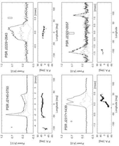
Figure 16: The polarization of millisecond pulsars at 1410 MHz from Xilouris98 . Four curves are plotted: the total power is shown by the outer curve in arbitrary units. The linear polarization is shown by the dashed curve and the circular polarization by the dotted curve. The linear polarization position angle is plotted on the lower panel in degrees. All curves are plotted against longitude in ms (upper scale) and in degrees (lower scale)

The discovery of millisecond pulsars Backer82 did not lead to immediate studies of their polarization. The first reports came in the 90’s Thorsett90 Navarro95 . This was due to the fact that millisecond pulsars are, on average, an order of magnitude less luminous than normal pulsars and thus require very sensitive polarimeters. A major contribution on millisecond pulsar polarimetry was published in 1998 Xilouris98 and more recently in 1999 Stairs99 . The polarization characteristics of millisecond pulsars are similar to those of normal pulsars, namely that the linear polarization falls to high frequencies Xilouris98 (Fig. 16).

5.2 Single Pulses

Most of the polarization observations presented so far referred to integrated pulses. However it is the polarization of the single pulse that tells us about constraints that are necessary for the interpretation of their emission mechanism. Early observations Rankin74 Manchester75b gave strong indications that pulsar radiation is highly polarized. Soon after a strange behaviour was also detected, e.g that orthogonal polarization modes, i.e. abrupt jumps of the position angle by $90{\hbox{${}^{\circ}$}}$ in consecutive single pulses are often observed Manchester75a Ganga97 .

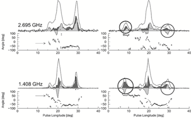
Figure 17: Two examples of individual pulse pairs of PSR B0329+54, observed in full polarization. The dark-shaded area represents linearly polarized power and the light-shaded area circularly polarized power. From Karastergiou01

In 1995 a major co-operation project was organized under the auspices of the European Pulsar Network. Various telescopes in Europe (Effelsberg, Jodrell Bank, Bologna, Westerbork, Torun and Pushchino) were used simultaneously to observe pulsars at a number of frequencies. Recently the radio telescopes in Ooty and GMRT (both in India) have joined this network. Each telescope was optimal at some frequency, so that a very wide frequency coverage was achieved. Many of the telescopes have the capability to observe the full polarization of pulsars as well. The results of this major multi-frequency network have shed new light on the wide band performance of pulsars as emitters Karastergiou01 Karastergiou02 Karastergiou03a Karastergiou03b Kramer03 . The fundamental result, that pulsar radio emission is basically broad-band, was confirmed. This is seen in Fig. 8 where single pulses observed at four widely spaced frequencies are plotted. Observations of full polarization showed even more unusual time sequences. While the total intensities correlated rather well, the polarization deviations were much higher. In particular the circular polarization (usually observed in the conal lobes of a pulse) vary highly from pulse to pulse (Fig. 17).

6 Distributions

More than 1500 pulsars have been discovered to date, facilitating the statistical investigation of their distribution in space, period, period derivative and in other parameter spaces. These distributions are by now statistically stable and reliable, not only because of the large number of stars involved in the sample but because they cover a large portion ($\sim$1%) of the pulsar population which is believed to be of the order of $10^{5}$ pulsars in our Galaxy. The figures presented below were produced using the data for 1300 pulsars available in the recently released ATNF pulsar catalogue (www.atnf.csiro.au/research/pulsar/psrcat/) Manchester03 . A few pulsars in the ATNF pulsar catalogue are X-ray pulsars. Among them there are some with long period. They have been included as their properties are very similar to normal radio pulsars.

6.1 Spatial distribution

Figure 18: The distribution of 1395 pulsars in Galactic Coordinates. Normal pulsars are depicted by dots. Binary pulsars have a large circle around them. Pulsars with p $<$ 20 msec are depicted by stars. Binary millisecond pulsars are shown by encircled stars. Figure courtesy of B. Klein

The distribution of pulsars in galactic coordinates is shown in Fig. 18 in Hammer-Aitoff projection. It is obvious that pulsars are strongly grouped along the galactic plane. Millisecond pulsars (many of which are also binary) are more isotropically distributed. This effect is due to their inherent weaker emission, which allows the detection of, primarily, nearby objects.

6.2 Dispersion Measure vs. Galactic Latitude distribution

Figure 19: The distribution of the Dispersion Measure of 1282 pulsars as a function of their Galactic Latitude

The Dispersion Measure (DM) of pulsars depicts the electron content on the line of sight, between the star and the observer, $\int{n_{e}(l)\times dl}$, where $n_{e}(l)$ is the electron density and l is the distance. If the average electron density is known, then the DM is a direct measure of the pulsar distance. From Fig. 19 it is obvious (a) that pulsars are tightly clustered along the galactic plane (galactic latitude, b = 0^∘) and (b) that the highest DMs are found on this plane. This is due to the electron density distribution in the Galaxy, which has been modelled by several researchers Lyne85 Taylor93 . According to these models, the electron density peaks at the Galactic centre and falls off with a scale height of about 70 parsecs away from the plane.

A few pulsars deviate from the smooth 1/e distribution. These objects are known to be located behind dense HII regions, e.g the Gum Nebula.

6.3 Period distribution

Figure 20: The period distribution of 1300 pulsars

Pulsar periods range from 1.5 ms to about 8.5 s (Fig. 20). This range of values for a physical parameter characterizing one species of objects is too wide to be explained by a common origin. It is widely accepted that ms pulsars are recycled pulsars, spun up by accretion processes, during which they accumulate mass and obtain extra spin (from this mass) from a binary component. This is confirmed by the data of Fig. 18, which show that most millisecond pulsars are in binary systems.

The histogram of pulsar periods shows a distinct bimodal distribution. The median of the period distribution of normal pulsars is about 0.65 s, whereas for millisecond pulsars it is 0.0043 s (4.3 ms). There is a characteristic lack of pulsars with period around 20 ms.

6.4 Period derivative ($\dot{P}$) distribution

The $\dot{P}$ distribution of pulsars (not shown, as it is directly connected to Figs. 20 and 21) varies between $10^{-21}$ $ss^{-1}$ to $10^{-10}$ $ss^{-1}$. Millisecond pulsars exhibit a much slower decay (lengthening) of their period. One of the fastest decaying period pulsars is the Crab pulsar, whose period slows down by 36 ns per day. In general the $\dot{P}$ distribution of pulsars is very similar to the period distribution.

There is a noticeable bimodal distribution. The median of the $\dot{P}$ distribution of normal pulsars is $2.6\times 10^{-15}$ $ss^{-1}$, whereas for millisecond pulsars it is of the order of $2\times 10^{-20}$ $ss^{-1}$. Five orders of magnitude slower period decay.

6.5 Period – Period derivative ($\dot{P}$) distribution

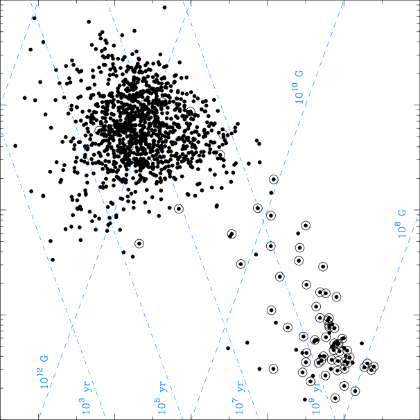
Figure 21: The P – $\dot{P}$ distribution of 1395 pulsars. Binary pulsars are depicted by encircled dots

One of the most important graphical distributions of pulsars is their period (P) – period derivative ($\dot{P}$) distribution (Fig. 21). As expected from Figures 20 and 22 it shows very clearly the characteristic clustering of normal pulsars (large P, large $\dot{P}$) and of millisecond pulsars (small P, small $\dot{P}$). The vast majority of normal pulsars are isolated single stars. On the contrary, the majority of millisecond pulsars are members of binary star systems. Binary pulsars located between the two clusters will slowly drift toward the millisecond cluster in less than $10^{8}$ years.

Assuming that the decay of pulsar periods is due to their dipole radiation, their characteristic age can be calculated from the very simple expression $\tau_{char}={1\over 2}{P\over\dot{P}}$ years. The “dash-dot” lines in Fig. 21 correspond to lines of constant age. The characteristic age of normal pulsars is of the order of $10^{8}$ years, whereas the age of millisecond pulsars is slightly above $10^{9}$ years. The Crab pulsar is the isolated pulsar closest to the $10^{3}$ years line.

Following classical electrodynamics theory, the surface magnetic field of pulsars is given by the expression $B_{0}=3.3\times 10^{19}\times\sqrt{P\dot{P}}$ gauss. The “dash” lines in Fig. 21 correspond to lines of constant magnetic field. It is immediately noted that normal pulsars have a surface magnetic field of about $10^{12}$ gauss, whereas the surface magnetic field of millisecond pulsars is much lower, of the order of $10^{9}$ gauss.

Finally it should be mentioned that the absence of pulsars in the lower right corner of the diagram is due to the existence of a “death line”, owing to the gradual decaying of the induced electrical potential of pulsars. Slow pulsars with low magnetic field cannot develop a large enough potential above their magnetic poles for discharges (and therefore radiation) to take place. The absence of millisecond pulsars below about $10^{10}$ years indicates that their age cannot exceed the Hubble time (age of the Universe).

Figure 22: The Age distribution of 1194 pulsars

6.6 Age distribution

The characteristic age ($\tau_{char}={1\over 2}{P\over\dot{P}}$) distribution of pulsars (Fig. 22) shows the expected bimodal distribution attributed to the different ages of normal pulsars and millisecond pulsars. The median age of normal pulsars is $4.7\times 10^{6}$ years, whereas the age of millisecond pulsars is of the order of $5\times 10^{9}$ years.

6.7 Surface Magnetic Field distribution

Figure 23: The surface magnetic field distribution of 1194 pulsars

The surface magnetic field ($B_{0}=3.3\times 10^{19}\times\sqrt{P\dot{P}}$) distribution of normal pulsars is tightly peaked at $1.3\times 10^{12}$ gauss, whereas for millisecond pulsars is much lower, of the order of $4\times 10^{8}$ gauss(Fig. 23). In a few stars the surface magnetic field is larger than $10^{14}$ gauss. This is the surface magnetic field of a new class of objects, called magnetars, first detected through their X-ray emission Kouveliotou98 . Magnetars are known to be neutron stars, which do not always emit at radio wavelengths.

6.8 Luminosity distribution

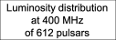
Figure 24: The luminosity distribution at 408 MHz of 612 pulsars

The luminosity distribution at 400 MHz of 612 pulsars is depicted in Fig. 24. The mean of the gauss fitted distribution is 115 $mJy\ kpc^{2}$. The luminosity is calculated from the 400 MHz flux density, assuming that the Dispersion Measure is a true measure of the distance of each pulsar. This may lead to an over estimate of the luminosity of pulsars located behind HII regions.

6.9 Spectral Index distribution

Figure 25: The spectral index distribution of 285 pulsars. Data between 400 MHz and 1400 MHz were used

The spectral index distribution between 400 MHz and 1400 MHz of 285 pulsars is shown in Fig. 25. It is a rather wide distribution. The bulk of pulsars demonstrate a spectral index between -3 and 0. The mean of the gauss fitted distribution is -1.75 $\pm$ 0.1. Pulsars with flat spectral indices are the ones which should be investigated at high frequencies.

Acknowledgements JHS acknowledges financial support from the Alexander von Humboldt Foundation and the Max-Planck-Gesellschaft during his sabbatical from the University of Thessaloniki. . We would like to acknowledge the fact that the publicly available ATNF pulsar catalogue of 1300 objects has given new momentum to pulsar research. We thank Dr. Axel Jessner for comments on an early version of this paper. Figures 18 and 21 were produced by Dr. Bernd Klein (Max-Planck-Institut für Radioastronomie, Bonn). Dr. Michael Kramer provided us with unpublished material which was used in some figures. Finally, we would like to thank an anonymous referee for useful comments.

References

- (1) Alpar M.A., Cheng A.F., Ruderman M.A., et al. 1982, A new class of radio pulsars. Nature, 300: 728–730
- (2) Arons J. 1993. Magnetic field topology in pulsars. Astrophys. J., 408: 160–166
- (3) Baade W., Zwicky F. 1934. Cosmic Rays from Super-Novae. Proc. Nat. Acad. Sci., 20:254
- (4) Baade W., Zwicky F. Remarks on Super-Novae and Cosmic Rays. Phys. Rev., 46: 76–77
- (5) Backer D.C. 1972. Pulsar flux-density spectra. Astrophys. J., 174: L157–L161
- (6) Backer D.C. 1976. Pulsar average wave forms and hollow-cone beam models. Astrophys. J., 209: 895–907
- (7) Backer D.C., Fisher J.R. 1974. Pulsar flux-density spectra. Astrophys. J., 189: 137–145
- (8) Backer D.C., Kulkarni S.R, Heiles C., Davis M.M., Goss W.M. 1982. A Millisecond Pulsar. Nature, 300: 615–618
- (9) Bartel N., Sieber W. 1978. Simultaneous single pulse observations of radio pulsars at two widely spaced frequencies. Astron. Astrophys., 70: 307–310
- (10) Bartel N., Sieber W., Wielebinski R. 1977. Detection of two pulsars at 22.7 GHz. Astron. Astrophys., 55: 319–320
- (11) Bartel N., Sieber W., Wielebinski R. 1978. Observations of pulsars at 14.8 and 22.7 GHz. Astron. Astrophys., 68: 361–365
- (12) Bartel N., Sieber W., Wielebinski R., Kardashev N. S., Nikolaev N. Ia., Popov M. V., Soglasnov V. A., Kuzmin A. D., Smirnova T. V. 1981. Simultaneous two-station single pulse observations of radio pulsars over a broad frequency range. I - With particular reference to PSR 0809+74. Astron. Astrophys., 93: 85–92
- (13) Becker W., Aschenbach B. 2002. X-ray observations of neutron stars and pulsars: First results from XMM-Newton. in Proceedings of the 270. WE-Heraus Seminar on: Neutron stars, Pulsars, and Supernovae, W. Becker W., H. Lesch, J. Trümper (eds) MPE Report 278, p.64–86
- (14) Bell Burnell S.J. 1979. Little Green Men, White Dwarfs or Pulsars?. http://www.bigear.org/vol1no1/burnell.htm
- (15) Beskin V.S., Gurevich A.V., Istomin Ya. N. 1986. Physics of pulsar magnetospheres. Cambridge University Press, Cambridge
- (16) Boriakoff V., Ferguson D.C. 1981. Microstructure cross-correlations in pulses observed at frequencies separated by 1 GHz. In Pulsars: 13 years of research on neutron stars, Proc. IAU Symp. 95, eds. W. Sieber & R. Wielebinski, pp. 191–196 . Dordrecht, Reidel, 1981
- (17) Boriakoff V., Ferguson D.C., Slater G. 1981. Pulsar microstucture quasiperiodicity. In Pulsars: 13 years of research on neutron stars, Proc. IAU Symp. 95, eds. W. Sieber & R. Wielebinski, pp. 199–204 . Dordrecht, Reidel, 1981
- (18) Brezgunov V.N., Udaltsov, V.A 1971. Spectra of pulsars CP 0950 and CP 1133 in the frequency range 83-111MHz. Astronom. Zh., 48: 14–18
- (19) Bruck Yu.M.; Ustimenko B.Yu.. 1973. Pulsars-Decametric emission from PSR 0809, PSR 1133, PSR 1919. Nature Phys. Sci., 242: 58–59
- (20) Callanan P.J, Garnavich P.M., Koester, D. 1998. The mass of the neutron star in the binary millisecond pulsar PSR J1012+5307. Mon. Not. R. Astr. Soc., 298: 207–211
- (21) Campbell D.B., Heiles C., Rankin J.M. 1970. Pulsar NP0532: Average polarization and daily variability at 430 MHz. Nature, 225: 527–528
- (22) Chadwick J. 1932. The existence of a neutron. Proc. Roy. Soc., 136: 692–708
- (23) Chadwick J. 1932. Possible existence of a neutron. Nature, 129: 312–312
- (24) Clark R.R., Smith F.G. 1969. Polarization of radio pulses from CP0328. Nature, 221: 724–726
- (25) Comella J.M., Craft Jr. H.D., Lovelace R.V.E., Sutton J.M., Tyler G.L. 1969. Crab Nebula pulsar NP0532. Nature, 221: 453–454
- (26) Cordes J.M. 1978. Observational limits on the location of pulsar emission regions. Astrophys. J., 222: 1006–1011
- (27) Craft H.D., Comella J.M., Drake F.D.. 1968. Submillisecond radio intensity variations in pulsars. Nature, 218: 1122–1124
- (28) CSIRO Media Release 1998. Parkes Telescope puts 1000 pulsar runs on the board. http://www.csiro.au/news/mediarel/mr1998/mr98259.html
- (29) Datta B., Ray A. 1983. Lower bounds on neutron star mass and moment of inertia implied by the millisecond pulsar. Mon. Not. R. Astr. Soc., 204: 75–80
- (30) Davies J.G., Horton P.W., Lyne A.G., Rickett B.J., Smith F.G., 1968. Pulsating radio source at , . Nature, 217: 910–912
- (31) Davies J.G., Lyne A.G., Smith F.G., Izvekova V.A., Kuzmin A.D., Shitov Iu.P. 1984. The magnetic field structure of PSR 0809 + 74. Mon. Not. R. Astr. Soc., 211: 57–68
- (32) Ekers R.D., Moffet A.T. 1968. Further observations of pulsating radio sources at 13cm. Nature, 220: 756–761
- (33) Ekers R.D., Moffet A.T. 1969. Polarization of Pulsating Radio Sources. Astrophys. J., 158: L1–L8
- (34) Erickson W.C., Mahoney M.J. 1985. The radio continuum spectrum of PSR 1937+214. Astrophys. J., 299: L29–L31
- (35) Ferguson D.C., Seiradakis J.H. 1978. A detailed, high time resolution study of high frequency radio emission from PSR 1133+16. Astron. Astrophys., 64: 27–42
- (36) Ferguson D.C., Graham D.A., Jones B.B., Seiradakis J.H., Wielebinski R. 1976. Direct observation of pulsar microstructure. Nature, 260: 25–27
- (37) Fishman G.J., Harnden F.R., Haymes R.C.. 1969. Observation of pulsed hard X-radiation from NP 0532 From 1967 data. Astrophys. J. Lett. 156: L107–L110
- (38) Fishman G.J., Harnden F.R., Johnson III W.N, Haymes R.C. 1969. The period and hard X-ray spectrum of NP 0532 in 1967. Astrophys. J. Lett., 158: L61–L64
- (39) Flowers E., Ruderman M.A. 1977. Evolution of Pulsar Magnetic Fields. Astrophys. J., 215: 302–310
- (40) Foster R.S., Fairhead L., Backer D.C. 1991. A spectral study of four millisecond pulsars. Astrophys. J., 378: 687–695
- (41) Gangadhara R.T. 1997. Orthogonal polarization mode phenomenon in pulsars. Astron. Astrophys., 327: 155–166
- (42) Gil J., Krawczyk A. 1997. PSR J0437-4715: a challenge for pulsar modelling. Mon. Not. R. Astr. Soc., 285: 561–566
- (43) Gil J., Sendyk M. 1999. Spark Model for Pulsar Radiation Modulation Patterns. Astrophys. J., 541: 351–366
- (44) Gil J., Kijak J., Seiradakis J.H. 1993. On the Two-Dimensional Structure of Pulsar Beams. Astron. Astrophys., 272: 268–276
- (45) Gold T. 1968. Rotating neutron stars as the origin of the pulsating radio sources. Nature, 218: 731–732
- (46) Goldreich P., Julian W.H. 1969. Pulsar Electrodynamics. Astrophys. J., 157: 869–880
- (47) Gould D.M, Lyne A.G. 1998. Multifrequency polarimetry of 300 radio pulsars. Mon. Not. R. Astr. Soc., 301: 235–260
- (48) Graham D.A., Lyne A.G., Smith F.G. 1970. Polarization of the radio pulses from the Crab Nebula pulsar. Nature, 225: 526–526
- (49) Haensel P., Zdunik J.L., Douchin F. 2002. Equation of state of dense matter and the minimum mass of cold neutron stars. Astron. Astrophys., 385: 301–307
- (50) Hamilton P.A., McCulloch P.M., Ables J.G., Komesaroff M.M. 1977. Polarization characteristics of southern pulsars. I - 400-MHz observations. Mon. Not. R. Astr. Soc., 180: 1–18
- (51) Hankins T.H. 1971. Microsecond intensity variations in the radio emissions from CP 0950 Astrophys. J., 169: 487–494
- (52) Hankins T.H., Kern J.S., Weatherell J.C., Eilek J.A. 2003. Nanosecond radio bursts from strong plasma turbulence in the Crab pulsar Nature, 422: 141–143
- (53) Helfand D.J., Manchester R.N., Taylor J.H. 1975. Observations of pulsar radio emission. III - Stability of integrated profiles Astrophys. J., 198: 661-670
- (54) Hewish A., Bell S.J, Pilkington J.D.H., et al. 1968, Observation of a Rapidly Pulsating Radio Source. Nature, 217: 709–713
- (55) Huguenin G.R., Taylor J.H., Hjellming R.M., Wade C.M. 1971. Interferometric observations of pulsars at 2.7 and 8.1 GHz. Nature Phys. Sci., 234: 50–51
- (56) Hulse R.A., Taylor J.H. 1975. Discovery of a pulsar in a binary system. Astrophys. J. Lett., 195: L51–L53
- (57) Jonker P.G., van der Klis M., Groot P.J. 2003. The mass of the neutron star in the low-mass X-ray binary 2A 1822 - 371. Mon. Not. R. Astr. Soc., 339: 663–668
- (58) Kalogera V., Baym G. 1996. The Maximum Mass of a Neutron Star. Astrophys. J., 470: L61–L64
- (59) Karastergiou A., von Hoensbroech A., Kramer M., Lorimer D.R., Lyne A.G., Doroshenko O., Jessner A., Jordan C., Wielebinski R. 2001. Simultaneous single-pulse observations of radio pulsars. I. The polarization characteristics of PSR B0329+54. Astron. Astrophys., 379: 270–278
- (60) Karastergiou A., Kramer M., Johnston S., Lyne A.G., Bhat N.D.R., Gupta Y. 2002. Simultaneous single-pulse observations of radio pulsars. II. Orthogonal polarization modes in PSR B1133+16 Astron. Astrophys., 391: 247–251
- (61) Karastergiou A., Johnston S., Kramer M. 2003. Simultaneous single-pulse observations of radio pulsars. III. The behaviour of circular polarization Astron. Astrophys., 404: 325–332
- (62) Karastergiou A., Johnston S., Mitra D., van Leeuwen A.G.J., Edwards R.T. 2003. V. New insight into the circular polarization of radio pulsars Mon. Not. R. Astr. Soc., 344: L69–L72
- (63) Karastergiou A., Jessner A., Wielebinski R. 2003. High Frequency Polarimetric Observations of the Crab Pulsar. In Young Neutron Stars and their Environment, Proc. IAU Symp. 218, eds. F. Camilo & B.M. Gaensler, p. 170
- (64) Kardashev N.S., Nikolaev N.Ya., Novikov A.Yu. Popov M.V., Soglasnov V.A., Kuzmin A.D., Smirnova T.V., Sieber W., Wielebinski R. 1986. Simultaneous single-pulse observations of radio pulsars over a broad frequency range. II - Correlation between intensities of single pulses at 102.5 and 1700 MHz. Astron. Astrophys., 163: 114–118
- (65) Kaspi V.M., Wolszczan A. 1993. A preliminary analysis of pulse profile stability in PSR 1257+12. In Planets around pulsars, eds. J.A. Philipps, J.E. Thorsett, S.R. Kulkarni, ASP Conf. Ser. 36, Princeton Univ., N.J., pp. 81–87
- (66) Kijak J., Kramer M., Wielebinski R., Jessner A. 1997. Observations of millisecond pulsars at 4.85 GHz. Astron. Astrophys., 318: L63–L66
- (67) Kijak J., Kramer M., Wielebinski R., Jessner A. 1998. Pulse shapes of radio pulsars at 4.85 GHz. Astron. Astrophys. Suppl. Ser., 127: 153–165
- (68) Komesaroff M.M. 1970.Possible mechanism for the pulsar radio emission. Nature, 225: 612–614
- (69) Kouveliotou,C., Dieters S., Strohmayer T., van Paradijs, J., Fishman G.J., Meegan C. A., Hurley, K., Kommers J., Smith I., Frail D., Murakami T. 1998. An X-ray pulsar with a superstrong magnetic field in the soft gamma-ray repeater SGR 1806-20. Nature, 393: 235–237
- (70) Kramer M. 1994. Geometrical analysis of average pulsar profiles using multi-component Gaussian fits at several frequencies. II. Individual results. Astron. Astrophys. Suppl. Ser., 107: 527–539
- (71) Kramer M., Wielebinski R., Jessner A., Gil J. A., Seiradakis J. H. 1994. Geometrical analysis of average pulsar profiles using multi-component Gaussian fits at several frequencies. I. Method and analysis. Astron. Astrophys. Suppl. Ser., 107: 515–526
- (72) Kramer M., Xilouris K.M., Jessner A., Wielebinski R., Tomofeev M. 1996. A turn-up in pulsar spectra at mm-wavelegths. Astron. Astrophys., 306: 867–876
- (73) Kramer M., Jessner A., Doroshenko O., Wielebinski R. 1997. Observations of pulsars at 7 millimetres. Astrophys. J., 488: 364–367
- (74) Kramer M., Xilouris K.M., Lorimer D.R., Doroshenko O., Jessner A., Wielebinski R., Wolszczan A., Camilo F. 1998. The characteristics of millisecond pulsars emission I. Spectra, pulse shapes and beaming fraction. Astrophys. J., 501: 270–285
- (75) Kramer M., Lange C., Lorimer D.R., Backer D.C., Xilouris K.M., Jessner A., Wielebinski R. 1999. The Characteristics of Millisecond Pulsar Emission. III. From Low to High Frequencies. Astrophys. J., 526: 957–975
- (76) Kramer M., Johnston S., van Straten W. 2002. High-resolution single-pulse studies of the Vela pulsar. Mon. Not. R. Astr. Soc., 334: 523–532
- (77) Kramer M., Karastergiou A., Gupta Y., Bhat N.D.R., Lyne A.G. 2003. Simultaneous single-pulse observations of radio pulsars: IV. Flux density spectra of individual pulses. Astron. Astrophys., 407: 655–668
- (78) Kuzmin A.D., Losovsky B.Ya. 2001. No low-frequency turn-over in the spectra of millisecond pulsars. Astron. Astrophys., 368: 230–238
- (79) Kuzmin A.D., Izvekova V.A., Shitov Yu.P., Sieber W., Jessner A., Wielebinski R., Lyne A.G., Smith F.G. 1998. Catalogue of time aligned profiles of 56 pulsars at frequencies between 102 and 10500 MHz. Astron. Astrophys. Suppl. Ser., 127: 355–366
- (80) Lange Ch., Kramer M., Wielebinski R., Jessner A. 1998. Radio pulsar microstucture at 1.41 and 4.85 GHz. Astron. Astrophys., 332: 111–120
- (81) Large M.I., Vaughan A.E., Mills B.Y. 1968. A pulsar supernova association. Nature, 220: 340–341
- (82) Large M.I., Vaughan A.E., Wielebinski R. 1968. Pulsar search at the Molonglo Radio Observatory. Nature, 220: 753–756
- (83) Lesch H., Jessner A., Kramer M., Kunzl T. 1998. On the possibility of curvature radiation from radio pulsars. Astron. Astrophys., 332: L21–L24
- (84) Löhmer O., Kramer M., Mitra D., Lorimer A.G., Lyne A.G. 2002. Anomalous scattering of highly dispersed pulsars. Astrophys. J., 562: L157–L161
- (85) Lorimer D.R., Yates J.A., Lyne A.G., Gould D.M. 1995. Multifrequency flux density measurements of 280 pulsars. Mon. Not. R. Astr. Soc., 273: 411–421
- (86) Lyne A.G., Burgay M., Kramer M. et al. 2004. A double-pulsar binary system - a rare laboratory for relativistic gravity and plasma physics . Science, in press
- (87) Lyne A.G., Manchester R.N. 1988. The shape of pulsar radio beams. Mon. Not. R. Astr. Soc., 234: 477–508
- (88) Lyne A.G., Rickett B.J. 1968. Measurement of the pulse shape and spectra of the pulsating radio sources. Nature, 218: 326–330
- (89) Lyne A.G., Smith F.G. 1968. Linear Polarization in Pulsating Radio Sources. Nature, 218: 124–126
- (90) Lyne A.G., Smith F.G. 1990. Pulsar Astronomy. Cambridge University Press. Cambridge
- (91) Lyne A.G., Manchester R.N., Taylor J.H. 1985. The galactic population of pulsars. Mon. Not. R. Astr. Soc., 213: 613–639
- (92) Malofeev V.A., Malov I.F. 1980. Mean spectra for 39 pulsars and the interpretation of their characteristic features Sov. Astron., 24: 54–62
- (93) Malofeev V.M., Gil J.A., Jessner A., Malov I.F., Seiradakis J.H., Sieber W., Wielebinski R. 1994. Spectra of 45 pulsars. Astron. Astrophys., 285: 201–208
- (94) Malofeev V.A., Malov I.F., Shchegoleva N.V. 2000. Flux density of 235 pulsars at 102.5 MHz. Astron. Rep., 44: 436–445
- (95) Malofeev V.M., Wielebinski R., Kramer M., Jessner A., Malov I., Malov O., Tyul’bashev S. 2003. Spectra of 48 millisecond pulsars in a wide frequency range Astron. Astrophys., submitted
- (96) Manchester R.N. 1971. Observations of Pulsar Polarization at 410 and 1665 MHz. Astrophys. J. Suppl. Ser., 23: 283–322
- (97) Manchester R.N. 1975. Orthogonal polarization in pulsar radio emission. PASA, 2: 334–336
- (98) Manchester R.N. 1995. The shape of pulsar beams. J. Astrophys. Astron., 295: 280–298
- (99) Manchester R.N., Taylor J.H. 1977. Pulsars. Freeman. San Francisco
- (100) Manchester R.N., Huguenin G.R., Taylor J.H. 1972. Polarization of the Crab Pulsar Radiation at Low Radio Frequencies. Astrophys. J., 174: L19–L23
- (101) Manchester R.N., Taylor J.H., Huguenin G.R. 1973. Frequency Dependence of Pulsar Polarization. Astrophys. J., 179: L7–L10
- (102) Manchester R.N., Taylor J.H., Huguenin G.R. 1975. Observations of pulsar radio emission. II - Polarization of individual pulses. Astrophys. J., 196: 83–102
- (103) Manchester R.N., Hamilton P.A., McCulloch P.M. 1980. Polarization characteristics of southern pulsars. III - 1612 MHz observations. Mon. Not. R. Astr. Soc., 16: 107–117
- (104) Manchester R.N., Han J.L., Qiao G.J. 1998. Polarization observations of 66 southern pulsars. Mon. Not. R. Astr. Soc., 295: 280–298
- (105) Manchester R.N., Hobbs G.B., Teoh A., Hobbs M. 2003. A New Pulsar Catalog. Astron. J., (submitted), presently at www.atnf.csiro.au/research/pulsar/psrcat/
- (106) Maron O., Kijak J., Kramer M., Wielebinski R. 2000. Pulsar spectra of radio emission. Astron. Astrophys. Suppl. Ser., 147: 195–203
- (107) Maron O., Kijak J., Wielebinski R. 2004. Observations of millisecond pulsars at 8.35 GHz. Astron. Astrophys., 413: L19–22
- (108) McCulloch P.M., Hamilton P.A., Manchester R.N., Ables J.G. 1978. Polarization characteristics of southern pulsars. II - 640-MHz observations. Mon. Not. R. Astr. Soc., 183: 645–676
- (109) Michel F.C. 1991. Theory of pulsar magnetospheres. Univ. of Chicago Press, Chicago
- (110) Mitra D., Deshpande A.A. 1999. Revisiting the shape of pulsar beams. Astron. Astrophys., 346: 906–912
- (111) Moffett D.A., Hankins T.H. 1996. Multifrequency Observations of the Crab Pulsar. Astrophys. J., 468: 779–783
- (112) Moffett D.A., Hankins T.H. 1999. Polarimetric Properties of the Crab Pulsar between 1.4 and 8.4 GHZ. Astrophys. J., 522: 1046–1052
- (113) Morris D., Schwarz U.J., Cooke D.J.. 1970. Measurements of the linear polarization of seven pulsars at 11-cm wavelength. Astrophys. Lett., 5: 181–186
- (114) Morris D., Graham D.A., Sieber W., Jones B.B., Seiradakis J.H. Thomasson, P. 1979. Intrinsic position angles of polarization for 40 pulsars. Astron. Astrophys., 73: 46–53
- (115) Morris D., Graham D.A., Sieber W., Bartel N., Thomasson, P. 1981. Observations of the polarization of average pulsar profiles at high frequency Astron. Astrophys. Suppl. Ser., 46: 421-472
- (116) Morris D., Kramer M., Thum C., Wielebinski R., Grewing M., Penalver J., Jessner A., Butin G., Brunswig W. 1997. Pulsar detection at 87 GHz Astron. Astrophys., 322: L17–L20
- (117) Navarro J., de Bruyn A.G., Frail D.A., Kulkarni S.R., Lyne A.G. 1995. A Very Luminous Binary Millisecond Pulsar. Astrophys. J., 455: L55–L58
- (118) Nollert H.-P., Ruder H., Herold H., Kraus U. 1988. Relativistic ‘Looks’ of a Neutron Star. Astron. Astrophys., 208: 153–156
- (119) Oppenheimer J.R., Volkoff G.M. 1939. On massive neutron cores. Phys.Rev., 55: 374–381
- (120) Oster L. & Sieber W. 1976. Pulsar geometries III: The hollow-cone model. Astrophys. J., 210: 220–229
- (121) Pacini F. 1967. Energy emission from a neutron star. Nature, 216: 567–568
- (122) Pandharipande V.R., Pines D., Smith R.A. 1976. Neutron star structure: theory observation and speculation. Astrophys. J., 208: 550–566
- (123) Psaltis D., Seiradakis J.H. 1996. The peculiar Moding of PSR 1237+25. In 2nd Hellenic astronomical conference : proceedings eds. M. Contadakis et al. Hellenic Astronomical Society, Greece, pp. 316–319
- (124) Qiao Guojun, Manchester R.N., Lyne A.G., Gould D.M. 1995. Polarization and Faraday rotation measurements of southern pulsars. Mon. Not. R. Astr. Soc., 274: 572–588
- (125) Radhakrishnan V., Cooke D.J. 1969. Magnetic poles and the polarization structure of pulsar radiation. Astrophys. Lett., 3: 225–229
- (126) Radhakrishnan V., Manchester R.N. 1969. Detection of a change of state in the pulsar PSR 083345. Nature, 222: 228–229
- (127) Rankin J.M. 1983. Toward an empirical theory of pulsar emission. I. Morphological taxonomy. Astrophys. J., 274: 333–358
- (128) Rankin J.M. 1983. Toward an empirical theory of pulsar emission. II - On the spectral behavior of component width Astrophys. J., 274: 359–368
- (129) Rankin J.M. 1986. Toward an empirical theory of pulsar emission. III - Mode changing, drifting supulses and pulse nulling Astrophys. J., 301: 901–922
- (130) Rankin J.M. 1993. Toward an empirical theory of pulsar emission. VI - The geometry of the conal emission region Astrophys. J., 405: 285–297
- (131) Rankin J.M. 1993. Toward an empirical theory of pulsar emission. VI - The geometry of the conal emission region: Appendix and tables. Astrophys. J. Suppl. Ser., 85: 145–161
- (132) Rankin J.M., Campbell D.B., Backer D.C. 1974. Individual Pulse Polarization Properties of three Pulsars Astrophys. J., 188: 609–614
- (133) Rankin J.M., Stinebring D.R. Weisberg J.M. 1989. Arecibo 21 centimeter polarimetry of 64 pulsars - A guide to classification. Astrophys. J., 346: 869–897
- (134) Richards D.W., Comella J.M. 1969. The period of pulsar NP 0532. Nature, 222: 551–552
- (135) Rickett B.J. 1969. Frequency structure of pulsar intensity variations. Nature, 221: 158–159
- (136) Rickett B.J., Hankins T.H., Cordes J.M. 1975. The radio spectrum of micropulses from pulsar PSR 0950+08. Astrophys. J., 201: 425–430
- (137) Robinson B.J., Cooper B.F.C., Gardner F.F., Wielebinski R., Landecker T.L. 1968. Measurements of the pulsed radio source CP1919 between 85 and 2700 MHz. Nature, 218: 1143–1145
- (138) Romani R.W. 1990. A Unified Model of Neutron–Star Magnetic Fields. Nature, 347: 741–743
- (139) Ruderman M.A., Sutherland P.G. 1975. Theory of pulsars - Polar caps, sparks, and coherent microwave radiation. Astrophys. J., 196: 51–72
- (140) Seiradakis J.H., Gil J.A., Graham D.A., Jessner A., Kramer M., Malofeev V.M., Sieber W., Wielebinski R. 1995. Pulsar profiles at high frequencies. I. The data. Astron. Astrophys. Suppl. Ser., 111: 205–227
- (141) Sieber W. 1973. Pulsar spectra: a summary Astron. Astrophys., 28: 237–252
- (142) Sieber W., Reinecke R., Wielebinski R. 1975. Observations of pulsars at high frequencies. Astron. Astrophys., 38: 169-182
- (143) Smith F.G. 1968. Measurement of the interstellar magnetic field. Nature, 218: 325–326
- (144) Srinivasan G. 2002. The maximum mass of neutron stars. Astron. Astrophys. Rev., 11: 67–96
- (145) Staelin D., Reifenstein E.C. 1969. Pulsating radio sources near the Crab Nebula Science, 162: 1481–1483
- (146) Stairs I.H, Thorsett S.E., Camilo F. 1999. Coherently Dedispersed Polarimetry of Millisecond Pulsars. Astrophys. J. Suppl. Ser., 123: 627–638
- (147) Stinebring D.R., Smirnova, T.V., Hankins T., Hovis J.S. Kaspi V.M.; Kempner J.C., Myers E., Nice D.J. 2000. Five Years of Pulsar Flux Density Monitoring: Refractive Scintillation and the Interstellar Medium. Astrophys. J., 539: 300–316
- (148) Taylor J.H., Cordes J.M. 1993. Pulsar distances and the galactic distribution of free electrons. Astrophys. J., 411: 674–684
- (149) Thorsett S.E., Chakrabarty D. 1999. Neutron Star Mass Measurements. I. Radio Pulsars. Astrophys. J., 512: 288–299
- (150) Thorsett S.E., Stinebring D.R. 1990. Polarimetry of millisecond pulsars. Astrophys. J., 361: 644–649
- (151) Thorsett S.E., Arzoumanian, Z., McKinnon M.M., Taylor J.H. 1993. The masses of two binary neutron star systems. Astrophys. J., 405: L29–L32
- (152) Time Magazine 1968. Astronomy: Fantastic Signals from Space. Time 15 March 1968: 36–36
- (153) Toscano M., Bailes M., Manchester R.N., Sandhu J.S. 1998. Spectra of southern Pulsars Astrophys. J., 506: 863-867
-
(154)
Unknown Daily Telegraph Science reporter.
1968. Bell-Burnell S.J., private communication. See also
http://www.nap.edu/readingroom/books/obas/contents/authorship.html - (155) von Hoensbroech A. 1999. The polarization of pulsar radio emission. Ph.D. Thesis Bonn University, Germany
- (156) von Hoensbroech A., Xilouris K.M. 1997. Effelsberg multifrequency pulsar polarimetry. Astron. Astrophys.S, 126: 121–149
- (157) von Hoensbroech A., Xilouris K.M. 1998. Does radius-to-frequency mapping persist close to the pulsar surface? Astron. Astrophys., 324: 981–987
- (158) Weber J. 1968. Gravitational radiation from pulsars. Phys. Rev. Lett., 21: 395–396
- (159) Weisberg J.M., Cordes J.M., Lundgren S.C., Dawson B.R., Despotes J.T., Morgan J.J., Weitz K.A., Zink E.C., Backer D.C. 1999. Arecibo 1418 MHZ Polarimetry of 98 Pulsars: Full Stokes Profiles and Morphological Classifications Astrophys. J. Suppl. Ser., 121: 171–217
- (160) Wielebinski R. 2002. Characteristics of (normal) pulsars at highest radio frequencies. In 270. WE-Heraeus Seminar on Neutron Stars, Pulsars and Supernova Remnants, eds. W. Becker et al., MPE Report 278: 167–171
- (161) Wielebinski R., Sieber W., Graham D.A., Hesse H., Schönhardt R.E 1972. Detection of six pulsars at 2.8 cm. Nature Phys. Sci., 240: 131–132
- (162) Wielebinski R., Jessner A., Kramer M., Gil J.A. 1993. First detection of pulsars at mm wavelengths. Astron. Astrophys., 272: L13–L16
- (163) Wolszczan A., Frail D.A. 1992. A planetary system around the millisecond pulsar PSR1257 + 12. Nature, 355: 145–147
- (164) Wu Xinji, Manchester R.N., Lyne A.G., Qiao Guojun 1993. Mean pulse polarization of southern pulsars at 1560 MHz. Mon. Not. R. Astr. Soc., 261: 630–646
- (165) Xilouris K.M., Rankin J.M., Seiradakis J.H., Sieber W. 1991. Polarimetric observations of 20 weak pulsars at 1700 MHz. Astron. Astrophys., 241: 87–97
- (166) Xilouris K.M., Seiradakis J.H., Gil J., Sieber W., Wielebinski R. 1995. Pulsar polarimetric observations at 10.55 GHz. Astron. Astrophys., 293: 153–165
- (167) Xilouris K.M., Kramer M., Jessner A., von Hoensbroech A., Lorimer D.R., Wielebinski R., Wolszczan A., Camilo F. 1998. The Characteristics of Millisecond Pulsar Emission. II. Polarimetry. Astrophys. J., 501: 286–306
- (168) Young M.D., Manchester R.N., Johnston S. A radio pulsar with an 8.5-second period that challenges emission models. 1999. Nature, 400: 848–849
- (169) Zhang B., Harding A.K. 2000. High Magnetic Field Pulsars and Magnetars: A Unified Picture. Astrophys. J., 535: L51–L54