LPT-ORSAY-04-48

Electroproduction Cross Section of Large-E_⊥ Hadrons

at NLO and Virtual Photon Structure Function

M. Fontannaz

Laboratoire de Physique Théorique, UMR 8627 CNRS,
Université Paris XI, Bâtiment 210, 91405 Orsay Cedex, France

We calculate Higher Order corrections to the resolved component of the electroproduction cross section of large-$E_{\bot}$ hadrons. The parton distributions in the virtual photon are studied in detail and a NLO parametrization of the latter is proposed. The contribution of the resolved component to the forward production of large-$E_{\bot}$ hadrons is calculated and its connection with the BFKL cross section is discussed.

1 Introduction

The electroproduction cross section of large-$E_{\bot}$ hadrons can be split up in two parts. One of them describes the reaction in which the initial virtual photon takes part directly in the hard scattering process ; it is called the direct part. But the photon can also act as a composite object which is a source of collinear partons which will take part in the hard subprocess ; this mechanism is usually refered to as the resolved process and defines the parton distributions in the virtual photon which have the feature of being proportional to $\ell n\ E_{\bot}^{2}/Q^{2}$ in the asympototic region where $E_{\bot}^{2}\gg Q^{2}$ (virtually $Q^{2}$ is the absolute value of the photon).

This distinction between direct and resolved component parts is especially useful in photoproduction reactions in which a quasi-real photon is present in the initial state (for a review, see ref. [1]). In this case the parton distributions in the real photon are proportional to $\ell n\ E_{\bot}^{2}/\Lambda_{QCD}^{2}$ and can be quite large. The interest in these real distributions dates from the pioneering work by Witten [2] who showed that their asymptotic behavior can be completely calculated in perturbative QCD, a result which opened the way to interesting tests of the theory. Nevertheless, when $E_{\bot}^{2}/\Lambda_{QCD}^{2}$ decreases, the importance of the non perturbative contributions grows and we return to a situation similar to that of the proton structure functions for which non perturbative inputs are necessary.

The situation is clearer when the initial photon is not real, but has a virtuality $Q^{2}$ much larger than $\Lambda_{QCD}^{2}$. In this case the non perturbative contributions (for instance that of the Vector Meson Dominance type) are suppressed by powers of $Q^{2}$ and we are back in the realm of perturbative QCD. The magnitude of the virtual distributions is smaller than that of the real distributions. Nonetheless, they are observable and dedicated experiments have studied the virtual parton distributions in $e^{+}e^{-}$ collisions [3, 4] and in the electroproduction of large $E_{\bot}$ jets [5, 6, 7] and hadrons [8, 9]. These studies acquire a quantitative status when data are compared with theoretical predictions calculated beyond the Leading Logarithm approximation [10, 11, 12, 13, 14]. It is the aim of this paper to establish such NLO expressions for the resolved component of the electroproduction of large-$E_{\bot}$ hadrons. We studied the corresponding direct component in ref. [15].

This work puts the theoretical predictions on a firmer ground since the full cross section formed by the direct and the resolved component parts is now calculated at the NLO approximation. In ref. [15] we founded predictions for the leptoproduction of forward large-$E_{\bot}$ hadrons on a NLO calculation of the direct term only. Then we observed that the resolved component, calculated at the lowest order, was not negligible. Here we pursue this study of the forward production now including the HO corrections to the resolved part. This allows us to refine our predictions and our comparisons with the BFKL-type cross section which should constitute a non negligible part of the forward cross section [16, 17].

In the next section we gather kinematical definitions and general expressions concerning the resolved cross section, including a discussion of the kinematical domain in which such a resolved component can be defined. Section 3 is devoted to the general structure of the NLO corrections and the issue of the factorization scheme. In Section 4 we propose a parametrization of the NLO parton distributions in the virtual photon, finally, we consider some numerical applications in Section 5.

2 The resolved component

In this section we present the kinematical definitions and the general expressions necessary for the study of the resolved component. This determines the frame in which the HO calculation described in the next section, will be performed. The cross section of the reaction $e(\ell)+p(P)\to e(\ell^{\prime})+h(P_{4})+X$,

$${d\sigma\over d\varphi dQ^{2}dy}={\alpha\over 2\pi}\ {1\over 2\pi}\ {1\over 2S}{1\over 2}\int{\ell^{\mu\nu}T_{\mu\nu}\over Q^{4}}\ dPS\ ,$$ (1)

is written in terms of the leptonic tensor $\ell^{\mu\nu}=2(\ell^{\mu}\ell^{\prime\nu}+\ell^{\nu}\ell^{\prime\mu}-g^{\mu\nu}(\ell\cdot\ell^{\prime}-m_{e}^{2}))$ and of the hadronic tensor $T_{\mu\nu}$ which describes the photon-proton collision. We define the photon variables $Q^{2}=-q^{2}=-(\ell-\ell^{\prime})^{2}$ and $y={q^{0}-q^{z}\over\ell^{0}-l^{z}}={P\cdot q\over P\cdot\ell}=Q^{2}/(x_{{\scriptscriptstyle B}_{j}}S)$ in a frame in which $P^{\mu}$ has no transverse component (we neglect the proton mass and $P^{z}$ is positive (HERA convention)). $S$ is given by $S=(P+\ell)^{2}$ and $x_{{\scriptscriptstyle B}_{j}}$ has the usual definition $x_{{\scriptscriptstyle B}_{j}}=Q^{2}/2P\cdot q$ ; $\varphi$ is the photon azimuthal angle. The differential phase space of the final hadrons is given by (a sum over the number of final hadrons is understood in (1))

$$dPS=(2\pi)^{4}\delta^{4}\left(q+P-\sum_{i=1}^{n}p_{i}\right)\prod_{i=1}^{n}{d^{4}p_{i}\over(2\pi)^{3}}\delta(p_{i}^{2})\theta(p_{i}^{0})\ .$$ (2)

The hadronic tensor can be calculated as a convolution between the partonic tensor $t_{\mu\nu}$ which describes the interaction between the virtual photon and the parton of the proton, and the parton distribution in the proton $G_{a}(x,M)$. The fragmentation of the final parton which produces a large-$E_{\bot}$ hadron is described by the fragmentation function $D_{b}^{h}(z,M_{F})$. These distributions depend on the factorization scales $M$ and $M_{F}$,

$$\int T_{\mu\nu}dPS=\sum_{a,b}\int{dx\over x}G_{a}(x,M)\int dz\ D_{b}^{h}(z,M_{F})t_{\mu\nu}^{ab}\cdot dps$$ (3)

where $dps$ is the phase space element of the partons produced in the hard photon-parton collision. From expressions (2) and (3), we obtain

$${d\sigma\over d\varphi dQ^{2}dydE_{\bot 4}d\eta_{4}}={E_{\bot 4}\over 2\pi}{\alpha\over 2\pi}\sum_{a,b}\int dxG_{a}(x,M)\int{dz\over z^{2}}D_{b}^{h}(z,M_{F})$$

$$\int{d\varphi_{4}\over 2\pi}\ {1\over(4\pi)^{2}}\ {1\over 2xS}\ {\ell^{\mu\nu}t_{\mu\nu}^{ab}\over q^{4}}\ dps^{\prime}$$ (4)

where the phase space $dps^{\prime}$ no longer contains parton 4 which fragments into $h(P_{4})$. ($\eta_{4}$ is the pseudo-rapidity of the observed hadron).

It is useful to give a more explicit form to the tensor product in the $\gamma^{*}-p$ frame by defining the transverse polarization vectors $\varepsilon_{1}^{\mu}=(0,1,0,0)$, $\varepsilon_{2}^{\mu}=(0,0,1,0)$ and the scalar polarization vector $\varepsilon_{s}^{\mu}={1\over\sqrt{Q^{2}}}(q^{z},0,0,q^{0})$ with $q^{\mu}=(q^{0},0,0,q^{z})$ the virtual photon momentum

$$\ell^{\mu\nu}t_{\mu\nu}=Q^{2}(t_{11}+t_{22})+4\left({Q^{2}(1-y)\over y^{2}}-m_{e}^{2}\right)t_{11}$$

$$+4{2-y\over y}\ell_{x}\sqrt{Q^{2}}\ t_{s1}+Q^{2}{4(1-y)\over y^{2}}t_{ss}\ ,$$ (5)

the transverse momentum $\ell_{x}$ of the initial lepton being along the $x$-axis.

In the limit $Q^{2}\to 0$ and after azimuthal averaging over $\varphi_{4}$ we recover the unintegrated Weizsäcker-Williams expression

$${1\over 2}\ {\ell^{\mu\nu}t_{\mu\nu}\over Q^{4}}=\left({1+(1-y)^{2}\over yQ^{2}}-{2y\ m_{e}^{2}\over Q^{4}}\right)\sigma_{\bot}+{\cal O}\left(\left(Q^{2}\right)^{0}\right)$$ (6)

with $\sigma_{\bot}={1\over 2y}\left(t_{11}+t_{22}\right)$.

Actually the limit (6) is correct only if $\lim\limits_{Q^{2}\to 0}t_{ss}={\cal O}(Q^{2})$. This is not true if an initial collinearity is present in the partonic tensor (light partons are massless) which leads to the behavior $\lim\limits_{Q^{2}\to 0}t_{ss}={\cal O}(1)$. This point is discussed at the end of this section.

The partonic tensor is given by a perturbative expression in $\alpha_{s}$. The Born contribution is of order ${\cal O}(\alpha_{s})$ and corresponds to the QCD Compton subprocess $\gamma^{*}+q\to g+q$ and the fusion process $\gamma^{*}+g\to q+\bar{q}$. Higher Order ${\cal O}(\alpha_{s}^{2})$ corrections to the Born cross section have been calculated in ref. [15]. In the course of these HO calculations a resolved component appears, corresponding to subprocesses in which the virtual photon creates a collinear $q$-$\bar{q}$ pair ; the quark or the antiquark subsequently interacts with a parton of the proton.

Let us study this contribution in detail by considering the simple model illustrated by the gauge invariant set of Feynman graphs displayed in Fig. 1. The neutral parton of momentum $p$ is off-shell and is part of a hard process also involving a parton of the proton. The final parton of momentum $p_{4}$ fragments into the observed large-$E_{\bot}$ hadron of transverse energy $E_{\bot 4}$. All the results described below can easily be obtained from the expressions given in appendix 1.

Figure 1: Feynman graphs leading to a resolved contribution.

The cross section corresponding to the graphs of Fig. 1 has double and single poles in $k^{2}=(q-k^{\prime})^{2}$. The interference term between graphs (a) and (b) has a single pole which leads to an expression proportional to $\ell n{p_{\bot 4}^{2}\over-q^{2}}$, after integration over $k^{\prime}_{\bot}$. However, a prefactor $q^{2}$ is present in all tensor components $t_{\scriptscriptstyle AB}$ (A, B$=S,1,2)$. As a result, these components have no singularities when $q^{2}$ tends to zero. This well-known behaviour is due to current conservation (for the components involving a scalar photon) and to the fact that interference terms are not singular for transverse photons. Therefore, let us concentrate on the square of graph (a) and start with the transverse component which has the expression (after integration over the azimuthal angle $\varphi_{k^{\prime}})$

$$t_{ii}={\alpha\over 2\pi}\ 3e_{f}^{2}\int dz\left[(1-z)^{2}+z^{2}\right]\int_{-q^{2}z}^{p_{\bot 4}^{2}/(1-z)}{dk^{2}\over k^{4}}\left\{zq^{2}-k^{2}\right\}{|\mu(0)|^{2}\over 2z}\quad(i=1,2)$$ (7)

where $\mu(0)$ is the hard subprocess amplitude, here representing the process $k+p\to p_{4}$, in which we have set $k^{2}$ and $k_{\bot}^{2}$ equal to zero. The upper limit of the $k^{2}$-integration indicates the scale at which the collinear approximation used in (7) by setting $k^{2}$ and $k_{\bot}^{2}$ equal to zero is no longer valid, using formulae (2) and (2), and after integration over $k^{2}$. The contraction with the leptonic tensor leads to

$${2\pi d\sigma\over d\varphi dQ^{2}dy}={\alpha\over 2\pi}\left[{1+(1-y)^{2}\over y}\ {1\over Q^{2}}-{2m_{e}^{2}y\over Q^{4}}\right]\int dz{\alpha\over 2\pi}\ 3e_{f}^{2}[(1-z)^{2}+z^{2}]$$

$$\cdot\left\{\ell n{p_{\bot 4}^{2}\over Q^{2}}-\ell n\ z-\ell n(1-z)-1\right\}\widehat{\sigma}\ ,$$ (8)

where we define $\widehat{\sigma}={|\mu(0)|^{2}\over 2zyS}$ (we have not written the contribution of order ${\cal O}(Q^{2}/p_{\bot 4}^{2})$). This expression is the lowest order resolved cross section and is exactly the one which is obtained in the course of the calculation of HO corrections to the direct Born terms [15]. The Weiszäcker-Williams distributions of the virtual photon in the initial electron and the quark distribution in the virtual photon are universal as they do not depend on the particular hard process described by cross-section $\widehat{\sigma}$. Expression (2) is the starting point of this paper. Indeed, when $\ell n{p_{\bot 4}^{2}\over Q^{2}}$ is large, one cannot content oneself with this approximation and corrections of the type $\alpha_{s}^{k}\left(\ell n{p_{\bot}^{4}\over Q^{2}}\right)^{n}$ with $k=n,n+1$ must be calculated and resummed. These corrections modify expression (2) at the Leading Order ($k=n$) and at the Next-to-Leading Order ($k=n+1$) approximation.

In order to avoid double counting, expression (2) must be subtracted from the NLO direct cross section. Actually the exact expression to be subtracted is a matter of factorization scheme. We define the resolved component by

$${2\pi d\sigma^{res}\over d\varphi dQ^{2}dy}={\alpha\over 2\pi}\left[{1+(1-y)^{2}\over y}\ {1\over Q^{2}}-{2m_{e}^{2}y\over Q^{4}}\right]\int dz{\alpha\over 2\pi}3e_{f}^{2}\left[(1-z)^{2}+z^{2}\right]\ell n{M_{\gamma}^{2}\over Q^{2}}\widehat{\sigma}$$ (9)

where we introduce the factorization scale $M_{\gamma}$ with $M_{\gamma}={\cal O}(E_{\bot 4})$. After subtraction, the part of (2) left in the direct HO corrections is obtained from (2) by the substitution $\ell n{p_{\bot 4}^{2}\over Q^{2}}\to\ell n{p_{\bot 4}^{2}\over M_{\gamma}^{2}}$. We call this factorization scheme the virtual factorisation scheme. This is a natural scheme in virtual photoproduction in which all the $\ell n\ Q^{2}$-terms are resummed in the parton distributions. Then the total NLO cross section is given by the sum of the subtracted direct cross section and of the resolved cross section calculated at NLO at the scale $M_{\gamma}$. The variations of the resolved cross section with $M_{\gamma}$ are partly compensated by the $\ell n\ M_{\gamma}^{2}$ terms, these remain in the direct cross section so that the total NLO cross section exhibits a smaller sensitivity to $M_{\gamma}$ than the LO cross section.

Of course this procedure is useful as long as $p_{\bot 4}^{2}\gg Q^{2}$. Actually the collinear approximation used in (7) is valid if $Q^{2}\ \raise 1.29167pt\hbox{$<$\kern-7.5pt\raise-4.73611pt\hbox{$\sim$}}\ k_{\bot}^{2}\ \raise 1.29167pt\hbox{$<$\kern-7.5pt\raise-4.73611pt\hbox{$\sim$}}\ p_{\bot 4}^{2}$, which allows us to put $k_{\bot}^{2}=0$ in the hard cross section. When $p_{\bot 4}^{2}\ \raise 1.29167pt\hbox{$<$\kern-7.5pt\raise-4.73611pt\hbox{$\sim$}}\ Q^{2}$, this upper limit is incorrect. Let us rewrite the $k^{2}$-integral in (7) in terms of $\vec{k}_{\bot}^{2}$

$$\int_{-q^{2}z}{dk^{2}\over|k^{2}|}\sigma(\vec{k}_{\bot}^{2})=\int_{0}{d\vec{k}_{\bot}^{2}\over k_{\bot}^{2}-q^{2}z(1-z)}\ \sigma(\vec{k}_{\bot}^{2})\ .$$ (10)

This integral is sensitive to the dependence on $\vec{k}_{\bot}^{2}$ of the $2\to 2$ subprocess cross section $\widehat{\sigma}(\vec{k}_{\bot}^{2})$ which behaves approximately like ${\cal O}({1\over(k_{\bot}+p_{\bot 4})^{2}})$. This behavior shows that no collinear logarithmic terms (coming from the denominator $\vec{k}_{\bot}^{2}+Q^{2}z(1-z)$) are present when $p_{\bot 4}^{2}\ \raise 1.29167pt\hbox{$<$\kern-7.5pt\raise-4.73611pt\hbox{$\sim$}}\ Q^{2}$. Therefore, the resolved component must be proportional to the result of $k_{\bot}^{2}$-integration in which the upper limit $p_{\bot 4}^{2}$ is replaced by $Q^{2}+p_{\bot 4}^{2}$. For $p_{\bot 4}^{2}\gg Q^{2}$ we have the case already discussed and for $p_{\bot 4}^{2}\ll Q^{2}$, there is no resolved component.

As a consequence it is more appropriate to define the factorization scale

$$M_{\gamma}^{2}=Q^{2}+C_{\gamma}^{2}E_{\bot 4}^{2}$$ (11)

($E_{\bot 4}$ is the transverse energy of the observed hadron) which has the following correct properties. 1) It does not depend on kinematical variables internal to the subprocess which may lead to incorrect results when HO corrections are calculated [19] ; 2) The resolved component calculated at $M_{\gamma}$ vanishes when $Q^{2}\gg E_{\bot 4}^{2}$ ; 3) again we find the conventional factorization scale $M_{\gamma}\simeq C_{\gamma}E_{\bot 4}$ when $E_{\bot 4}^{2}\gg Q^{2}$, $C_{\gamma}$ being an arbitrary constant of order 1.

Let us finish this section by discussing the tensor components $t_{is}$ and $t_{ss}$ which come from the square of graph (a) in Fig. 1. The components $t_{is}$ behave like $\sqrt{q^{2}}\ell n{p_{\bot 4}^{2}\over-q^{2}}$ and have no singularity at the limit $q^{2}\to 0$. On the contrary $t_{ss}$ has a constant behavior when $q^{2}\to 0$

$$t_{ss}={\alpha\over 2\pi}3e_{f}^{2}\int dz\ 4z(1-z)\int_{-q^{2}z}^{p_{\bot 4}^{2}/(1-z)}{d|k|^{2}\over k^{4}}(-q^{2}){|\mu(0)|^{2}\over 2}\ ,$$

or

$$t_{ss}={\alpha\over 2\pi}3e_{f}^{2}\int dz\ 4z(1-z)\left(1-{-q^{2}z(1-z)\over p_{\bot 4}^{2}}\right){|\mu(0)|^{2}\over 2z}\ ,$$ (12)

a result which leads to the scalar cross section

$${2\pi d\sigma^{scalar}\over d\varphi dQ^{2}dy}={\alpha\over 2\pi}\ {2(1-y)\over y}\ {1\over Q^{2}}\int dz\ {\alpha\over 2\pi}\ 3e_{f}^{2}\ 4z(1-z)\widehat{\sigma}\ .$$ (13)

In going from (12) to (13), we dropped the $-q^{2}z(1-z)/p_{\bot 4}^{2}$ term which depends, through $p_{\bot 4}$, on the detailed kinematics of the subprocess.

We observe that $t_{ss}$ has a “constant” behavior when $q^{2}\to 0$ due to the double pole of the cross section. Actually the limit $q^{2}\to 0$ corresponds to a non perturbative region for the $k^{2}$-integration. If instead of $|k^{2}_{min}|=-q^{2}z$ we set $|k_{min}^{2}|\sim\Lambda_{QCD}^{2}$, we would obtain a vanishing cross section when $q^{2}\to 0$. A similar result is obtained if we consider massive quarks (with $|k^{2}_{min}-m^{2}|=-q^{2}z+{m^{2}\over 1-z}$). Therefore, for a physical process and a real photon, there is no $t_{ss}$ contribution, as can be expected.

However, let us notice that for small values of $Q^{2}\sim\Lambda_{QCD}^{2}$, the resolved cross sections, as defined in (2) and (13), strongly depend on the way the $k^{2}$-integral is regularized, different lower bounds produce different $z$-dependence, and thus different physical results even when $E_{\bot 4}^{2}/Q^{2}$ is large. This paradox is however solved by the HO correction to parton distributions in the photon discussed in the next section. There we shall see that the NLO parton distributions contain a term that cancels the unwanted $z$-dependent contribution, up to a vanishing term when $E_{\bot 4}^{2}/Q^{2}$ tends to infinity. Actually this result is true for all $z$-dependent terms of collinear origin (related to the lower limit of the $k^{2}$-integration) present in (2) and (11). As a consequence the scalar cross section (13) will be cancelled.

3 NLO corrections

In section 2 we defined the resolved component of the transverse cross section $(i=1,2)$. (Here $\widehat{\sigma}^{B}$ is defined as the Born amplitude squared divided by the flux factor $z$).

$$t_{ii}={\alpha\over 2\pi}\ e_{f}^{2}\int dz\ P_{q\gamma}^{(0)}(z)\ell n{M_{\gamma}^{2}\over Q^{2}}\ \widehat{\sigma}^{B}$$ (14)

where the factorization scale is given by (11) and $P_{q\gamma}^{(0)}(z)=3[z^{2}+(1-z)^{2}]$ (for 1 quark species). Expression (14) contains the lowest order (${\cal O}(\alpha_{s}^{0})$) parton distributions in the virtual photon

$$q(z,M_{\gamma}^{2},Q^{2})={\alpha\over 2\pi}\ e_{f}^{2}\ P_{q\gamma}^{(0)}(z)\ell n{M_{\gamma}^{2}\over Q^{2}}\ .$$ (15)

The Born cross section $\widehat{\sigma}^{B}$ describes the scattering between a quark of the virtual photon and a parton of the proton producing two large-$p_{\bot}$ partons in the final state.

Leading Logarithm (LL) corrections, corresponding to the emission of collinear gluons by the initial quark, can be obtained by solving the following inhomogeneous DGLAP equation [18, 19] (we only reproduce the evolution equation for the Non Singlet (NS) quark distribution $q_{f}^{NS}=q_{f}+\overline{q}_{f}-\sum\limits_{f=1}^{N_{f}}(q_{f}+\overline{q}_{f})/N_{f}$) with $<e_{f}^{2}>=\sum\limits_{f}e_{f}^{2}/N_{f}$

$$M^{2}\ {\partial q_{f}^{NS}(M^{2},z)\over\partial M^{2}}={\alpha\over 2\pi}\ 2[e_{f}^{2}-<e_{f}^{2}>]\ P_{q\gamma}^{(0)}(z)+{\alpha_{s}(M^{2})\over 2\pi}\int_{z}^{1}{dz^{\prime}\over z^{\prime}}\ P_{qq}^{(0)}\left({z\over z^{\prime}}\right)q_{f}^{NS}(M^{2},z^{\prime})$$ (16)

where $P_{qq}^{(0)}(z)=C_{F}((1+z^{2})/(1-z))_{+}$. The lowest order expression (15) is solution of such an equation when $P_{qq}^{(0)}$ is set equal to zero. The solution of (16) for the moments $q_{f}^{NS}(M^{2},Q^{2},n)=\int_{0}^{1}dz\ z^{n-1}\ q^{NS}(M^{2},Q^{2},z)$ is given by ($d(n)=2P_{qq}^{(0)}(n)/\beta_{0}$ and $\beta_{0}$ is the lowest order coefficient of the $\beta$-function expansion ${\partial\alpha_{s}\over\partial\ell n(\mu^{2})}=\beta(\alpha_{s})\cong-{\alpha_{s}^{2}\over 4\pi}\beta_{0}$)

$$q_{f}^{NS,LL}(M^{2},Q^{2},n)={4\pi\over\alpha_{s}(M^{2})}\ {\alpha\over 2\pi}\ {2(e_{f}^{2}-<e_{f}^{2}>)P_{q\gamma}^{(0)}(n)\over\beta_{0}(1-d(n))}\left(1-\left({\alpha_{s}(M^{2})\over\alpha_{s}(Q^{2})}\right)^{1-d(n)}\right)$$ (17)

with the boundary condition $q_{f}^{NS,LL}(Q^{2},Q^{2},n)=0$. The Leading Logarithm NS expression for the resolved cross section is now given by

$$t_{ii}^{LL}=q_{f}^{NS,LL}\otimes\widehat{\sigma}^{B}\ ,$$ (18)

which is expression (14) in which the lowest order parton distribution is replaced by the LL solution (17).

The next step is to look for a Next to Leading Order (NLO) expression for $t_{ii}$, which requires the calculations of HO corrections to both $q^{LL}$ and $\widehat{\sigma}^{B}$. Indeed the structure of these HO corrections is the following. The hard cross section has the expression ($\widehat{\sigma}^{B}$ is of order ${\cal O}(\alpha_{s}^{2})$)

$$\widehat{\sigma}^{NLO}=\widehat{\sigma}^{B}+\alpha_{s}^{3}B$$ (19)

whereas the parton distributions behave, in the asymptotic domain $M_{\gamma}^{2}/Q^{2}\gg 1$, like

$$q^{NLO}={a\over\alpha_{s}(M_{\gamma}^{2})}+b\ .$$ (20)

It is clear from (19) and (20) that a NLO expression for $t_{ii}$ can only be obtained by calculating both $\alpha_{s}^{2}B$ and $b$.

3.1 The hard resolved cross section at NLO

The calculation of the HO corrections to the hard resolved cross section is the simpler part of the NLO program, since these HO are the same in real and virtual photoproduction reactions, providing we work in the same factorization scheme. Therefore, we can borrow the results of ref. [20] obtained for the real photoproduction of large $E_{\bot}$ hadrons.

Let us elaborate this point by first studying the resolved Born term. In the real case, instead of (7) we obtain the following expression

$$t_{ii}={\alpha\over 2\pi}\ 3e_{f}^{2}\int dz\left[z^{2}+(1-z)^{2}-\varepsilon\right]{(4\pi\mu^{2})^{\varepsilon}\over(1-\varepsilon)}\ {\Gamma(1-\varepsilon)\over\Gamma(1-2\varepsilon)}\int_{0}^{p_{\bot 4}^{2}}{dk_{\bot}^{2}\over(k_{\bot}^{2})^{1+\varepsilon}}\widehat{\sigma}_{\varepsilon}^{B}$$ (21)

in which we use the dimensional regularization and $n=4-2\varepsilon$. The expression between the square brackets is the $n$-dimensional DGLAP branching function ; the factor $(4\pi)^{\varepsilon}\Gamma(1-\varepsilon)/(\Gamma(1-2\varepsilon)(1-\varepsilon))$ comes from the azimuthal integration and the $n$-dimensional photon spin average. After integration over $k_{\bot}^{2}$, we obtain $(1/\overline{\varepsilon}={1\over\varepsilon}+\ell n\ 4\pi-\gamma_{E})$

$$t_{ii}={\alpha\over 2\pi}\ e_{f}^{2}\int dz\left(-{1\over\overline{\varepsilon}}+\ell n{M_{\gamma}^{2}\over\mu^{2}}\right)P_{q\gamma}^{(0)}(z)\widehat{\sigma}_{\varepsilon}^{B}+{\alpha\over 2\pi}\ e_{f}^{2}\int dz$$

$$\left(\ell n{p_{\bot 4}^{2}\over M_{\gamma}^{2}}P_{q\gamma}^{0}(z)-P_{q\gamma}^{0}(z)+3\right)\widehat{\sigma}^{B}$$ (22)

where the limit, when $\varepsilon$ tends to zero, of the $n$-dimension Born cross section $\widehat{\sigma}_{\varepsilon}^{B}$ is simply $\widehat{\sigma}^{B}$ of expression (14). This expression is identical to that obtained in the calculation of the HO corrections to the real direct term.

At this point, if we subtract the term proportional to $\left(-{1\over\varepsilon}+\ell n{M_{\gamma}^{2}\over\mu}\right)$ from (3.1), which defines the $\overline{\rm MS}$ factorization scheme, we obtain a direct HO subtracted contribution different from the one found in the virtual case (cf. expressions (2) and (9)). However, as we shall see in the next subsection, this scheme dependence is compensated by the NLO corrections to the parton distributions.

Now let us go one step further and consider ${\cal O}(\alpha_{s})$ corrections to the resolved expression (9). These HO corrections are the same in the real and in the virtual case, with the exception of collinear contributions coming from the branching $\gamma^{*}\to q+\overline{q}+g$ and containing $(\ell n\ p_{\bot 4}^{2}/Q^{2})^{n}$ $(n=1,2)$ terms. These logarithmic terms can be factorized and resummed at the NLO approximation with the result (we consider only the Non Singlet case)

$$q_{\gamma}^{NLO}(M_{\gamma}^{2},Q^{2})\otimes\left(1+{\alpha_{s}\over 2\pi}h_{qq}+{\alpha_{s}\over 2\pi}\ P_{qq}^{(0)}\ell n{p_{\bot 4}^{2}\over M_{\gamma}^{2}}\right)\otimes\widehat{\sigma}^{B}$$ (23)

where $\otimes$ indicates convolutions in the longitudinal variable. The factor 1 in the parenthesis corrsponds to the Born contribution (9). The term ${\alpha_{s}\over 2\pi}h_{qq}\otimes\widehat{\sigma}^{B}$ is the collinear HO correction calculated in the virtual factorization scheme (resummation of all the $\ell n\ Q^{2}$ terms in the parton distribution function with the boundary condition $q_{\gamma}^{NLO}(Q^{2},Q^{2})=0$). However the physical (direct + resolved) cross section is factorization scheme invariant and can be written in terms of the $\overline{\rm MS}$ quantities $\overline{q}_{\gamma}^{NLO}$ and $\overline{h}_{qq}(z)$. As a result we can use the HO correction calculated in ref. [20] in the $\overline{\rm MS}$ scheme if we also use parton distributions (and a direct term) calculated in the same scheme.

The authors of ref. [12, 13, 14] also worked in the $\overline{\rm MS}$ scheme in their study of the electroproduction of large-$p_{\bot}$ jets, and they established the expression which must be subtracted from the virtual direct term in order to obtain the $\overline{\rm MS}$ direct term. We comment on their results at the end of section 3.2.

3.2 The virtual parton distributions at NLO

In order to delimit the problem of the Factorization Scheme (FS) in the virtual parton distributions, we study the simple case of the DIS on a virtual photon and we consider the $n$-moment of the structure function ${\cal F}_{2}^{\gamma}=F_{2}^{\gamma}(x,K^{2},Q^{2})/x$ in which $Q^{2}=|q^{2}|$ is the virtuality of the target photon, $K^{2}=|k^{2}|$ is the virtuality of the probe photon and $x$ the Bjorken variable. To make the connection with the transverse cross section defined in (7), ${\cal F}_{2}^{\gamma}$ is defined by an average over the transverse spin of the target photon only. To simplify the discussion we only consider the Non Singlet contribution. ${\cal F}_{2}^{\gamma}$ is the sum of a resolved part and a direct part (we drop the indices $n$)

$${\cal F}_{2}^{\gamma}(K^{2},Q^{2})=C_{2,q}(\alpha_{s}(K^{2}))\cdot q_{\gamma}^{NS}(K^{2},Q)+C_{2,\gamma}^{NS}(\alpha_{s}(K^{2}))\ .$$ (24)

In (24) ${\cal F}_{2}^{\gamma}$ is proportional to $\sum\limits_{f=1}^{N_{f}}e_{f}^{2}[e_{f}^{2}-<e^{2}>]$ ; we drop this factor which is useless in the present discussion. The direct part, $C_{2,\gamma}^{NS}$, and the resolved hard cross section $C_{2,q}$ (the Wilson coefficient) are expansions in $\alpha_{s}(K^{2})$. All the $\ell n\ Q^{2}$ dependent terms are collected in the virtual quark distribution $q_{\gamma}^{NS}$ with the boundary condition $q_{\gamma}^{NS}(Q^{2},Q^{2})=0$. This defines the virtual factorization scheme already mentioned in section 2. In fact (24) is the final result obtained by Uematsu and Walsh [10] in their study of the virtual photon structure function, using the OPE and the MS factorization scheme as a starting point. The distribution $q_{\gamma}^{NS}$ verifies the inhomogeneous DGLAP equation (16) in which the lowest order branching function $P_{q\gamma}^{(0)}$ and $P_{qq}^{(0)}$ must be replaced by the all order functions $P_{q\gamma}^{NS}(\alpha_{s}(M_{\gamma}^{2}))$ and $P^{NS}(\alpha_{s}(M^{2}))={\alpha_{s}(M^{2})\over 2\pi}P_{qq}^{(0)}+\cdots$ which are expansions in $\alpha_{s}(M^{2})$ and depend on the factorization scheme. The solution of (16) can be written (from now on we drop the index NS)

$$q_{\gamma}(K^{2},Q^{2})={\alpha\over 2\pi}\int_{\alpha_{s}(Q^{2})}^{\alpha_{s}(K^{2})}{d\alpha^{\prime}\ P_{q\gamma}(\alpha^{\prime})\over\beta(\alpha^{\prime})}\ e^{\int_{\alpha^{\prime}}^{\alpha_{s}(K^{2})}{d\alpha^{\prime\prime})\over\beta(\alpha^{\prime\prime})}P(\alpha^{\prime\prime})}\ .$$ (25)

${\cal F}_{2}^{\gamma}$, being a physical observable, must be FS scheme invariant and cancellation must exist in (24) between the various scheme dependent contributions. Let us first note that $C_{2,\gamma}(K^{2})$ is FS scheme invariant because

$${\cal F}_{\gamma}^{2}(Q^{2},Q^{2})=C_{2,\gamma}(\alpha_{s}(Q^{2}))\ .$$ (26)

To study the scheme dependence of $q_{\gamma}$, let us start from expression (25) and define a new DGLAP branching function $\overline{P}$ by

$$P=\overline{P}-\delta P$$ (27)

where $\delta P$ is an arbitrary expansion in $\alpha_{s}$ starting at order ${\cal O}(\alpha_{s}^{2})$

$$q_{\gamma}(K^{2},Q^{2})={\alpha\over 2\pi}\ e^{-\int_{0}^{\alpha_{s}(K^{2})}{d\alpha^{\prime\prime}\over\beta(\alpha^{\prime\prime})}\delta P(\alpha^{\prime\prime})}\cdot\widetilde{q}_{\gamma}(K^{2},Q^{2})$$ (28)

with $\widetilde{q}_{\gamma}$ given by

$$\widetilde{q}_{\gamma}(K^{2},Q^{2})\equiv\int_{\alpha_{s}(Q^{2})}^{\alpha_{s}(K^{2})}{d\alpha^{\prime}\over\beta(\alpha^{\prime})}\left[P_{q\gamma}(\alpha^{\prime})e^{\int_{0}^{\alpha^{\prime}}{d\alpha^{\prime\prime}\over\beta(\alpha^{\prime\prime})}\delta P(\alpha^{\prime\prime})}\right]\cdot e^{\int_{\alpha^{\prime}}^{\alpha_{s}(K^{2})}{d\alpha^{\prime\prime}\over\beta(\alpha^{\prime\prime})}\overline{P}(\alpha^{\prime\prime})}\ .$$ (29)

We see that the variation $\delta P$ can be absorbed in $C_{2,q}$ (the hard resolved subprocess) and $P_{q\gamma}$, thus defining new expansions in $\alpha_{s}$, $\overline{C}_{2,q}(\alpha_{s}(K^{2}))$ and $\widetilde{P}_{q\gamma}(\alpha^{\prime})$, whereas ${\cal F}_{2}^{\gamma}$ is kept unchanged

$${\cal F}_{2}^{\gamma}(K^{2},Q^{2})=\overline{C}_{2,q}(\alpha_{s}(K^{2}))\widetilde{q}_{\gamma}(K^{2},Q^{2})+C_{2,\gamma}(\alpha_{s}(K^{2}))\ .$$ (30)

Let us now study the effects of modifying $\widetilde{P}_{q\gamma}$

$$\widetilde{P}_{q\gamma}=\overline{P}_{q\gamma}-\delta P_{q\gamma}$$ (31)

with the arbitrary series $\delta P_{q\gamma}$ starting at order ${\cal O}(\alpha_{s})$

$$\widetilde{q}_{\gamma}(K^{2},Q^{2})=\overline{q}_{\gamma}(K^{2},Q^{2})-{\alpha\over 2\pi}\int_{\alpha_{s}(Q^{2})}^{\alpha_{s}(K^{2})}{d\alpha^{\prime}\over\beta}\delta P_{q\gamma}\ e^{\int_{\alpha^{\prime}}^{\alpha_{s}(K^{2})}{d\alpha^{\prime\prime}\over\beta}\overline{P}}$$ (32)

where the parton distribution $\overline{q}_{\gamma}$ is calculated in the bar-scheme

$$\overline{q}_{\gamma}(K^{2},Q^{2})={\alpha\over 2\pi}\int_{\alpha_{s}(Q^{2})}^{\alpha_{s}(K^{2})}{d\alpha^{\prime}\over\beta}\overline{P}_{q\gamma}\ e^{\int_{\alpha^{\prime}}^{\alpha_{s}(K^{2})}{d\alpha^{\prime\prime}\over\beta}\overline{P}}\ .$$ (33)

Finally for ${\cal F}_{\gamma}^{2}$ we obtain the expression

$${\cal F}_{2}^{\gamma}(K^{2},Q^{2})=\overline{C}_{2,q}(\alpha_{s}(K^{2}))\left(\overline{q}_{\gamma}(K^{2},Q^{2})+q_{\gamma}^{B}(K^{2},Q^{2})\right)+\overline{C}_{2,\gamma}(\alpha_{s}(K^{2}))$$ (34)

where

$$\overline{C}_{2,\gamma}(\alpha_{s}(K^{2}))=C_{2,\gamma}(\alpha_{s}(K^{2}))-\overline{C}_{2,q}(\alpha_{s}(K^{2})){\alpha\over 2\pi}\int_{0}^{\alpha_{s}(K^{2})}{d\alpha^{\prime}\over\beta}\delta P_{q\gamma}\ e^{\int_{\alpha^{\prime}}^{\alpha_{s}(K^{2})}{d\alpha^{\prime\prime}\over\beta}\overline{P}}$$ (35)

and

$$q_{\gamma}^{B}(K^{2},Q^{2})={\alpha\over 2\pi}\int_{0}^{\alpha_{s}(Q^{2})}{d\alpha^{\prime}\over\beta}\delta P_{q\gamma}\ e^{\int_{\alpha^{\prime}}^{\alpha_{s}(K^{2})}{d\alpha^{\prime\prime}\over\beta}\overline{P}}\ .$$ (36)

Therefore in the new factorization scheme (the bar-scheme), the structure of the expression for ${\cal F}_{2}^{\gamma}$ is the same as in the original scheme, but the parton distribution does not vanish at $K^{2}=Q^{2}$ since $q_{\gamma}^{B}(Q^{2},Q^{2})$ is different from zero. Therefore, by going from the virtual FS to the bar-scheme, we find the boundary condition that the bar-distribution must verify. By rewriting (36) as

$$q_{\gamma}^{B}(K^{2},Q^{2})=e^{\int_{\alpha_{s}(Q^{2})}^{\alpha_{s}(K^{2})}{d\alpha^{\prime}\over\beta(\alpha^{\prime})}\overline{P}}\ {\alpha\over 2\pi}\int_{0}^{\alpha_{s}(Q^{2})}{d\alpha^{\prime}\over\beta(\alpha^{\prime})}\delta P_{q\gamma}\ e^{\int_{\alpha^{\prime}}^{\alpha_{s}(Q^{2})}{d\alpha^{\prime\prime}\over\beta(\alpha^{\prime\prime})}\overline{P}}\ ,$$ (37)

we see that $q_{\gamma}^{B}(K^{2},Q^{2})$ verifies the homogeneous DGLAP equation and that the boundary condition is given, at the lowest order ($\overline{P}={\alpha_{s}\over 2\pi}P_{qq}^{(0)}$, $\beta(\alpha_{s})=-{\alpha_{s}^{2}\over 4\pi}\beta_{0}$ and $\delta P_{q\gamma}={\alpha_{s}\over 2\pi}\delta P_{q\gamma}^{(1)}$), by

$$q_{\gamma}^{B}(Q^{2},Q^{2})=-{\alpha\over 2\pi}\ {\delta P_{q\gamma}^{(1)}\over P_{qq}^{(0)}}\ .$$ (38)

The bar-scheme can be any scheme, but it is convenient to work in the $\overline{\rm MS}$ factorization scheme in which the two-loop branching functions $P_{q\gamma}^{NS}$ and $P^{NS}$ are known. Moreover, in the electroproduction of large-$p_{\bot}$ hadrons we also know the NLO resolved subprocess cross section (the equivalent of $\overline{C}_{2,q}$) calculated in the $\overline{\rm MS}$ scheme in ref. [20]. It is easy to obtain $\delta P_{q\gamma}^{(1)}$ from expression (35) written at the lowest order on $\alpha_{s}$

$$\overline{C}_{2,\gamma}-C_{2,\gamma}={\alpha\over 2\pi}\ {\delta P_{q\gamma}^{(1)}\over P_{qq}^{(0)}}\ .$$ (39)

$\overline{C}_{2,\gamma}$ is the $\overline{\rm MS}$ direct term [22] and $C_{2,\gamma}$ is the virtual-scheme direct term [10]

$$C_{2,\gamma}={\alpha\over 2\pi}6\left\{8x(1-x)-2+\left(x^{2}+(1-x)^{2}\right)\ell n{1\over x^{2}}\right\}\ ,$$ (40)

which leads to

$$q_{\gamma}^{B}(Q^{2},Q^{2})=-{\alpha\over 2\pi}6\left\{\left(x^{2}+(1-x)^{2}\right)\ell n[x(1-x)]+1\right\}\ .$$ (41)

Let us finish this section by going back to the direct cross section of large-$p_{\bot}$ hadron electroproduction. The $\overline{\rm MS}$ boundary condition can be obtained by comparing expression (2) calculated in the virtual case and expression (3.1) corresponding to the real case. We see that subtracting $(z^{2}+(1-z)^{2})\ell n{1\over z(1-z)}-1$ from the virtual expression, we find the $\overline{\rm MS}$ expression $1-(z^{2}+(1-z))$. The term that we subtracted is equal to (41) as can be expected.

3.3 The scalar parton distribution at HO

In section 2 we found a scalar resolved contribution (13) to the electroproduction cross section corresponding to the scalar distribution $q_{0}^{S}(z)={\alpha\over 2\pi}3e_{q}^{2}[4z(1-z)]$. HO corrections to this distribution correspond to the Feynman graph

Figure 2: A higher order correction to the Feynman graphs of fig. 1.

of Fig. 2 (with an extra gluon in comparison to Fig. 1). Working in the LL approximation and considering only terms proportional to $\ell n\ K^{2}/Q^{2}$), we have

$$q_{1}^{S}(x,K^{2},Q^{2})=\int dz\ q_{0}^{S}(z)\int dz^{\prime}\ {\alpha_{s}\over 2\pi}\ P_{qq}^{(0)}(z^{\prime})\ \delta(zz^{\prime}-x)\ell n\ K^{2}/Q^{2}\ ,$$ (42)

or $q_{1}^{S}(n,K^{2},Q^{2})=q_{0}^{S}(n){\alpha_{s}\over 2\pi}P_{qq}^{(0)}(n)\ell nK^{2}/Q^{2}$. The full LL expression $q^{S}(n)=\sum\limits_{k=1}^{\infty}q_{k}^{S}(n)$ is easily resummed

$$q^{S}(n,K^{2},Q^{2})=\int_{\alpha_{s}(Q^{2})}^{\alpha_{s}(K^{2})}{d\alpha^{\prime}\over\beta(\alpha^{\prime})}q_{0}^{S}(n)\ {\alpha^{\prime}\over 2\pi}P_{qq}^{(0)}(n)\ e^{\int_{\alpha^{\prime}}^{\alpha_{s}(K^{2})}{d\alpha^{\prime\prime}\over\beta(\alpha^{\prime\prime})}{\alpha^{\prime\prime}_{s}\over 2\pi}P_{qq}^{(0)}}\ .$$ (43)

This solution is similar to expression (25), but with an inhomogeneous branching function starting at order ${\cal O}(\alpha_{s})$ ; it can be written

$$q^{S}(n,K^{2},Q^{2})=-q_{0}^{S}(n)\left[1-\left({\alpha_{s}(K^{2})\over\alpha_{s}(Q^{2})}\right)^{-2P_{qq}^{(0)}/\beta_{0}}\right]\ .$$ (44)

Adding this contribution to the lowest order one (13), we see that the latter is cancelled and replaced by a contribution which vanishes asymptotically because of the factor $(\alpha_{s}(K^{2})/\alpha_{s}(Q^{2}))^{-2P_{qq}^{(0)}/\beta_{0}}$. Therefore the scalar contribution (13) which is target dependent (it depends on the regularization of the $k^{2}$-integral as discussed in section 2) is cancelled. This mechanism is actually quite general and also valid for the transverse component.

Therefore, in the electroproduction case a full treatment of the scalar cross section amounts to subtract expression (13) from the NLO direct cross-section and to add the scalar resolved component

$${d\sigma^{scalar}\over d\varphi dQ^{2}dy}={\alpha\over 2\pi}\ {2(1-y)\over y}\ {1\over Q^{2}}\int dz\ q_{\gamma}^{S}(z,M_{\gamma}^{2},Q^{2})\widehat{\sigma}$$ (45)

where we define

$$q_{\gamma}^{S}(n,M_{\gamma}^{2},Q^{2})=q_{0}^{S}(n)\left({\alpha_{s}(M_{\gamma}^{2})\over\alpha_{s}(Q^{2})}\right)^{-2P_{qq}^{0}/\beta_{0}}\ .$$ (46)

4 NLO parametrization of the virtual photon structure function

Although the works of Uematsu and Walsh [10] and Rossi [25] date back to the eighties, interest in the virtual photon structure function grew much later, thanks to the HERA experiments. Since then several papers have been published discussing the parton distributions in virtual photons at the LL approximation [26, 27, 28] and NLO approximation [29, 30, 31], and emphasizing the possibility to measure them in electroproduction experiments [13, 14, 32, 33, 34, 35, 36]. In this section we present a study of the parton distributions in virtual photons performed in the $\overline{\rm MS}$ scheme, using the results of section 3 on the inputs at $K^{2}=Q^{2}$. We choose $Q^{2}$ large enough to neglect non perturbative effects, and therefore we do not present results on the limit $Q^{2}\to 0$. A NLO study has also been done by authors of refs. [29] and [30] in the DIS_γ scheme with emphasis the real limit $Q^{2}\to 0$. We may note however that the solutions of [30] do not fulfil condition (26) of section 3.

The parton distributions are solutions of the same NLO inhomogeneous differential equations as in the real case. The NS equation is given by expressions (16) in which ${\alpha\over 2\pi}P_{q\gamma}^{(0)}$ and ${\alpha_{s}\over 2\pi}P_{qq}^{(0)}$ must be replaced by NLO (two loops) DGLAP kernels ; the equations of the singlet sector as well as the expressions of the kernels can be found in ref. [21]. The only change with respect to the real case is the starting point of the evolution, $Q^{2}$ instead of $Q_{0}^{2}\sim(.5)^{2}$ GeV² in the real case. The boundary condition for the distributions are given by expression (41) for the quark distributions and we have $g_{\gamma}^{B}(Q^{2},Q^{2})=0$ for the gluon distributions. Another difference from the real case is the existence of a scalar contribution. The latter has been discussed in section 3.3.

In section 3 we studied the massless case $m_{q}^{2}\ll Q^{2}$. However $\sqrt{Q^{2}}$ can be smaller than the bottom mass $m_{b}$ and we have to determine what are the relevant boundary conditions for the bottom quark distribution in the virtual photon. To find these, let us introduce in expression (7) the kinematic corresponding to the case in which the photon interacts with a massive quark.

$$3\int_{Q^{2}z+{m^{2}\over 1-z}}^{p_{\bot 4}^{2}/(1-z)}{d|k^{2}-m^{2}|\over(k^{2}-m^{2})^{2}}\left\{|k^{2}-m^{2}|{z^{2}+(1-z)^{2}\over z}+{2m^{2}z-Q^{2}z(z^{2}+(1-z)^{2})\over z}\right\}$$

$$={1\over z}\left\{P_{q\gamma}(z)\ell n{p_{\bot 4}^{2}\over m^{2}+Q^{2}z(1-z)}+6z(1-z)-{3Q^{2}z(1-z)\over m^{2}+Q^{2}z(1-z)}\right\}\ .$$ (47)

We notice that for $m^{2}=0$, we find the massless corrections already given in (2) which are associated with the virtual factorization scheme.

For $Q^{2}=0$, we find

$${1\over z}\left\{P_{q\gamma}(z)\ \ell n{p_{\bot 4}^{2}\over m^{2}}+6z(1-z)\right\}$$ (48)

which is the $\overline{\rm MS}$ correction (once the term $\ell n{M_{\gamma}^{2}\over m^{2}}$ is subtracted). Therefore, in the massive case ($Q^{2}=0$) we directly work in the $\overline{\rm MS}$-scheme and we do not have to modify the factorization scheme as discussed in section 3. Therefore, there exists a transition between case $Q^{2}\gg m^{2}$ and case $Q^{2}\ll m^{2}$ that we should study in detail.

Let us start from expression (4). When $Q^{2}<m^{2}$, we factorize $P_{q\gamma}\ell n{M_{\gamma^{2}}\over m^{2}}$ which is the contribution given by the evolution equation starting at the scale $m^{2}$. The rest is given by (without the $1/z$ prefactor)

$$P_{q\gamma}\ell n{p_{\bot 4}^{2}\over M_{\gamma}^{2}}+6z(1-z)+MC_{<}(m^{2},Q^{2};z)$$ (49)

with

$$MC_{<}(m^{2},Q^{2};z)=P_{q\gamma}\ \ell n{m^{2}\over m^{2}+Q^{2}z(1-z)}-{3\cdot Q^{2}z(1-z)\over m^{2}+Q^{2}z(1-z)}\ ,$$

namely the usual masless $\overline{\rm MS}$ correction and corrections in $Q^{2}/m^{2}$. When $Q^{2}>m^{2}$, we factorize $P_{q\gamma}\ell n{M_{\gamma}^{2}\over Q^{2}}$ and we obtain

$$P_{q\gamma}\ \ell n{p_{\bot 4}^{2}\over M_{\gamma}^{2}}+P_{q\gamma}\ell n{1\over z(1-z)}+6z(1-z)-3+MC_{>}(m^{2},Q^{2};z)$$ (50)

with

$$MC_{>}(m^{2},Q^{2};z)=P_{q\gamma}\ell n{Q^{2}z(1-z)\over m^{2}+Q^{2}z(1-z)}+{3\cdot m^{2}\over m^{2}+z(1-z)Q^{2}}\ .$$

We recognize the massless corrections in the virtual scheme and a massive $m^{2}/Q^{2}$ correction.

However the same massive corrections $MC_{\displaystyle{\mathrel{\mathop{>}_{\textstyle<}}}}(m^{2}Q^{2};z)$ appear in the calculation of the inhomogeneous kernel $k_{q}^{(1)}$ as outlined in section 3.3. When we add the resolved and the direct contributions, these massive corrections are cancelled and are replaced by $MC_{<}(m^{2},Q^{2};n)(\alpha_{s}(M_{\gamma})^{2}/\alpha_{s}(m^{2}))^{-2P_{qq}^{(0)}/\beta_{0}}$ or by $MC_{>}(m^{2},Q^{2};n)(\alpha_{s}(M_{\gamma}^{2})/$$\alpha_{s}(Q^{2}))^{-2P_{qq}^{(0)}/\beta_{0}}$ when $Q^{2}>m^{2}$. In the latter case, we still have to add $-[P_{q\gamma}(z)\ell nz(1-z)+3]$ to $MC_{>}(m^{2},Q^{2};z)$ to move to the $\overline{\rm MS}$ scheme with the result

$$MC_{>}(m^{2},Q^{2};z)=P_{q\gamma}\ell n{Q^{2}\over m^{2}+Q^{2}z(1-z)}-{3Q^{2}z(1-z)\over m^{2}+Q^{2}z(1-z)}$$ (51)

which is equal to $MC_{<}(m^{2},Q^{2};z)$ when $m^{2}=Q^{2}$.

Therefore, we can summarize our treatment of the massive quarks in the following way. First we assume that the $m^{2}/E_{\bot 4}^{2}$ corrections are properly taken into account in the direct term (or that they are negligible when $E_{\bot 4}^{2}\gg m^{2})$. Second, we work in the massless $\overline{\rm MS}$ scheme and we take into account mass corrections through the input of the quark distributions. Thus we have the following inputs for $m_{c}^{2}\leq Q^{2}\leq m_{b}^{2}$ (up to charge factors)

$$\left.\begin{array}[]{l}u(x,Q^{2})\\ d(x,Q^{2})\\ s(x,Q^{2})\end{array}\right\} \sim-P_{q\gamma}\ \ell n\ x(1-x)-3$$

$$c(x,Q^{2}) \sim P_{q\gamma}\ \ell n\ {Q^{2}\over m_{c}^{2}+Q^{2}z(1-z)}-{3Q^{2}z(1-z)\over m_{c}^{2}+Q^{2}z(1-z)}$$

$$b(x,m_{b}^{2}) \sim P_{q\gamma}\ \ell n\ {m_{b}^{2}\over m_{b}^{2}+Q^{2}z(1-z)}-{3Q^{2}z(1-z)\over m_{b}^{2}+Q^{2}z(1-z)}\ .$$ (56)

Whereas for $Q^{2}\geq m_{b}^{2}$, we have the input

$$b(x,Q^{2})\sim P_{q\gamma}\ \ell n\ {Q^{2}\over m_{b}^{2}+Q^{2}z(1-z)}-{3Q^{2}z(1-z)\over m_{c}^{2}+Q^{2}z(1-z)}\ .$$ (57)

With these inputs we obtain the distributions shown in Fig. 3. We have chosen $Q^{2}=8$ GeV² and $M_{\gamma}^{2}=25$ which correspond to average values of $Q^{2}$ and $M_{\gamma}^{2}=Q^{2}+E_{\bot 4}^{2}$ of the H1 experiment [8]. The distributions calculated in the $\overline{\rm MS}$ scheme increase for $x$ going to one as we can see from Fig. 3. This increase is compensated however by the behavior of the direct term which contains terms in $\ell n(1-z)$ that become negative at large $z$. We also remark the effect of the massive input (4) for the charm quark distribution.

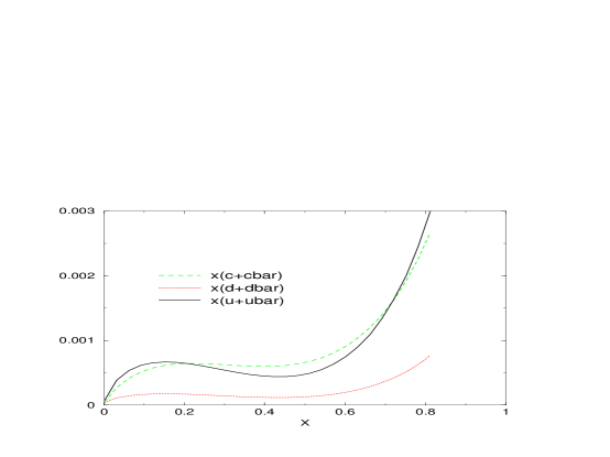
Figure 3: The parton distributions in the virtual photon for $Q^{2}=8$ GeV² and $M_{\gamma}^{2}=25$ GeV².

We end this section by comparing our results with experimental data obtained by the L3 collaboration [4] for the structure function

$$F_{eff}^{\gamma}=F_{2,\bot}^{\gamma}+F_{2,s}^{\gamma}$$ (58)

where the indices $\bot$ and $s$ refer to polarization of the target photon of virtuality $Q^{2}$ (called $P^{2}$ in ref. [4]). In terms of these components, the usual structure function $F_{2}^{\gamma}$ is written (the tensor indices refer to the target current) $F_{2}^{\gamma}=-{1\over 2}g^{\alpha\beta}(F_{2}^{\gamma})_{\alpha\beta}=F_{2,\bot}^{\gamma}-{1\over 2}F_{2,s}^{\gamma}$. Until now we calculated only the transverse distributions (Fig. 3) ; in order to obtain $F_{eff}^{\gamma}$ we have to add to $F_{2,\bot}^{\gamma}$ the scalar contribution defined in expression (46) for the quark component, in which a gluon distribution is also generated by the DGLAP evolution equation. All our calculations are done in the $\overline{\rm MS}$ scheme.

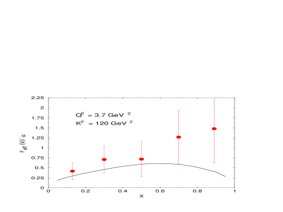
Figure 4: The structure function $F_{eff}^{\gamma}/\alpha$ compared to L3 data [4] with $Q^{2}=3.7$ GeV² and $K^{2}=120$ GeV². Statistical and systematical errors are added linearly.

In Fig. 4 we see that our predictions are in reasonable agreement with data at low and medium values of $x$, but they undershoot them at large values of $x$. Similar results have been obtained by the authors of ref. [11].

5 Numerical results

We now turn to a phenomenological study of the Deep Inelastic Production of large-$E_{\bot}$ hadrons. We concentrate mainly on the resolved contribution studied in this paper and consider the H1 data [8] already discussed in ref. [15] devoted to the direct contribution. This allows us to make a connection between the results presented here and those obtained in [15]. A more complete phenomenological study of the new H1 data [9] will be presented in a future paper [37], in which we shall also discuss in detail the link between the present NLO cross section and the cross section based on the exchange of Reggeized gluons [38] in the $t$-channel [16, 17]

As in paper [15], we use the MRST 99 (upper gluon) distributions for the parton in the proton [39] and the KKP fragmentation functions [40]. The strong coupling constant is given by an exact solution of the two loop-renormalization group equation and we use $\Lambda_{\overline{MS}}^{(4)}$ = 300 MeV. We take $N_{f}=4$. Our calculations are performed at $\sqrt{S}=$ 300.3 GeV and the forward-$\pi^{0}$ cross section is defined with the following cuts. In the laboratory system a $\pi^{0}$ is observed in the forward direction with $5^{\circ}\leq\theta_{\pi^{0}}\leq 25^{\circ}$ ; the laboratory momentum of the pion is constrained by $x_{\pi^{0}}=E_{\pi^{0}}/E_{P}\geq.01$, and an extra cut is put on the $\pi^{0}$ transverse momentum in the $\gamma^{*}-p$ center of mass system : $E_{\bot\pi^{0}}^{*}>2.5$ GeV. The inelasticity $y=Q^{2}/x_{{\scriptscriptstyle B}_{j}}S$ is restricted to the range $.1<y<.6$. We consider only the contribution coming from transversely polarized virtual photons, we shall comment briefly on the scalar contribution below.

Our numerical results obtained for the distribution $d\sigma/dx_{{\scriptscriptstyle B}_{j}}$ measured by H1 [8] in the range 4.5 GeV${}^{2}\leq Q^{2}\leq 15$ GeV² are shown in Fig. 5. In order to shorten the numerical calculation we do not integrate over $Q^{2}$, but instead use the average value of $Q^{2}$, $<Q^{2}>=8$ GeV², over the above range. We use the scale $Q^{2}+E_{\bot 4}^{2}$ in the entire series of calculations and we work in the $\overline{\rm MS}$ factorization scheme.

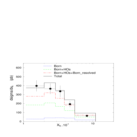
Figure 5: The cross section $d\sigma/dx_{{\scriptscriptstyle B}_{j}}$ corresponding to the range $4.5$ GeV${}^{2}\leq Q^{2}\leq 15$ GeV² compared to H1 data [8].

The direct HO corrections from which the resolved contribution is subtracted, called HO_s, are different from those obtained in ref. [15] in which we work in the virtual factorization scheme. In both schemes they are very large. In ref. [15] we noticed that the largest contribution to these corrections comes from the subprocesses $\gamma^{*}+g\to g+q+\overline{q}$ and $\gamma^{*}+q\to q+q+\overline{q}$. The sum of the HO_s contributions and of the resolved Born contribution should be factorization scheme independent, up to ${\cal O}(\alpha_{s})$ corrections. To check this point, let us consider the bin $2.9\cdot 10^{-4}\leq x_{{\scriptscriptstyle B}_{j}}\leq 3.9\cdot 10^{-4}$. In ref. [15] we used the virtual factorization scheme and we obtained $d\sigma/dx_{{\scriptscriptstyle B}_{j}}=155.5$ nb $+52.5$ nb = 208.0 nb for the sum. Note that the parton distributions used in that case are simply the lowest order distributions (15) without QCD evolution. In the $\overline{\rm MS}$ scheme we have $d\sigma/dx_{{\scriptscriptstyle B}_{j}}=125.9$ nb $+95.9$ nb = 221.8 nb, but we use the NLO parton distributions. One can check that the small difference between the two sums comes mainly from the gluon distributions not present in the lowest order expression. If we only use the quark $\overline{\rm MS}$ NLO distributions, we obtain $d\sigma^{Re}/dx_{{\scriptscriptstyle B}_{j}}=83.1$ nb for the resolved contribution and $d\sigma/dx_{{\scriptscriptstyle B}_{j}}=209$ nb for the sum. This result shows that the QCD evolution is negligible in this kinematical range (besides the generation of a small gluon distribution) and that expression (15) gives a good description, in the virtual factorization scheme, of the parton distributions in a virtual photon. A similar observation has been made by the authors of ref. [12] in the case of jet production. Because of this small evolution, we also have $q_{\gamma}^{2}(n,M_{\gamma}^{2},Q^{2})\simeq q_{0}^{S}(n)$. Therefore, it is not necessary to subtract the scalar resolved component from the direct term and to introduce a scalar (QCD evolved) resolved contribution.

The next point to observe from Fig. 5 is the importance of the HO resolved corrections compared to the Born resolved contributions, leading to a ratio $NLO/Born\simeq~{}2$ independent of $x_{{\scriptscriptstyle B}_{j}}$. These large HO corrections correspond to a small value of $E_{\bot 4}$ due to the small cut-off $E_{\bot\pi^{0}}^{*}\geq 2.5$ GeV. For a larger cut-off, for instance $E_{\bot\pi^{0}}^{*}\geq 5$ GeV, we obtain $NLO/Born=1.65$ in the range $2.9\cdot 10^{-4}\leq x_{{\scriptscriptstyle B}_{j}}\leq 3.9\cdot 10^{-4}$.

The total cross section is in good agreement with data, slightly overshooting them at $x_{B}\ \raise 1.29167pt\hbox{$>$\kern-7.5pt\raise-4.73611pt\hbox{$\sim$}}\ 4\cdot 10^{-4}$, and little room appears to be left for a BFKL-type contribution [17]. However this last statement depends on the scale used in the calculation, here $M=M_{\gamma}=M_{F}=\mu=(Q^{2}+E_{\bot 4}^{2})^{1\over 2}$, because the cross section strongly depends on the scale $\mu$. In ref. [15] we found that this was due to the importance of the subprocesses $\gamma^{*}+g\to g+q+\overline{q}$ and $\gamma^{*}+q\to q+q+\overline{q}$ with a gluon exchanged in the $t$-channel. These processes correspond to the opening of new channels that are not present at the Born level. They are of order ${\cal O}(\alpha_{s}^{2})$ and sensitive to the value of $\mu$ since there is no loop contributions at this order to compensate the $\mu$-dependence. However, this remark is not true for the resolved part of these subprocesses as soon as HO corrections for the resolved cross section are calculated. For instance the subprocess $\gamma^{*}+g\to g+q+\overline{q}$ contains a resolved lowest order contribution $(\gamma^{*}\to q\overline{q})+g\to g+q+\overline{q}$ ; loop corrections to this contribution, corresponding to HO corrections to the resolved cross section, generate counter terms in $\ell n{E_{\bot 4}^{2}\over\mu^{2}}$ ; these in turn compensate the $\mu$-dependence of the Born cross section. To check this point let us again consider the bin $2.9\cdot 10^{-4}\leq x_{{\scriptscriptstyle B}_{j}}\leq 3.9\cdot 10^{-4}$. Keeping $M=M_{\gamma}=M_{F}=(Q^{2}+E_{\bot 4}^{2})^{1\over 2}$ fixed and $E_{\bot\pi^{0}}^{*}>5$ GeV, we vary $\mu=C\sqrt{Q^{2}+E_{\bot 4}^{2}}$ with $C$ ranging from .15 to 1.0. The variations with $\mu^{2}$ of the Born and NLO resolved cross section are shown in Fig. 6.

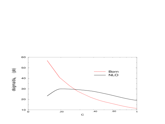
Figure 6: The variation with $\mu=C\sqrt{Q^{2}+E_{\bot 4}^{2}}$ of the resolved cross section.

We see that the behavior of the Born cross section and that of the NLO cross section are quite different. The latter has a maximum around $C\simeq.2$ and is more stable with respect to the variations of $C$ than the Born contribution. This behavior does not occur for the NLO direct contribution which always increases when $C$ decreases. Let us also note that this behavior cannot be observed for the cut $E_{\bot\pi^{0}}^{*}>2.5$ GeV. The HO corrections are too large and we cannot reach a maximum of the NLO cross section, even for very small values of $C$.

Let us conclude this section by noting another difference with respect to the direct term in which the large contributions to the forward cross section come from subprocesses involving the exchange of one elementary gluon in the $t$-channel. In the resolved case, the elementary gluon becomes reggeized, due to the HO corrections. Therefore, the resolved cross section contains contributions corresponding to the exchange of a reggeized gluon in the $t$-channel.

6 Conclusion

In this paper we calculated HO corrections to the resolved part of the DIS cross section for the production of large-$E_{\bot}\pi^{0}$. This involves the calculations of the HO corrections to parton distributions in the virtual photon (of virtuality $Q^{2}$) and of the HO corrections to the resolved subprocess.

We discuss the issue of the factorization scheme in detail and we establish the inputs of the parton distributions in the $\overline{\rm MS}$ scheme. Then the NLO parton distributions are obtained by solving the DGLAP inhomogeneous evolution equation. They are confronted to LEP data.

Our results for the NLO cross section are compared with H1 data for the production of forward large-$E_{\bot\pi^{0}}$. We find a good agreement with data, once the direct contribution is added to the resolved one. This result is obtained for renormalization and factorization scales equal to $Q^{2}+E_{\bot\pi^{0}}^{2}$. In a study of the scale sensitivity, we find that the resolved cross section is less sensitive to the renormalization scale than the direct cross section. It is interesting to notice that the authors of ref. [14] obtained very similar results in their NLO study of the electroproduction of large-$E_{\bot}$ forward jets.

We conclude that the good agreement between the NLO calculations and data leaves little room, in this kinematical range, for a BFKL-type contribution which resums a ladder of reggeized gluon.

Appendix 1

The square of the graphs in Fig. 1 possess single and double poles in $k^{2}$. Actually, as explained in section 2, the only relevant quantity is the square of graph (a) $S^{\mu\nu}/k^{4}$. Let us isolate the hard subprocess amplitude $\mu$ by using the projector defined in ref. [41] ${I\hskip-2.84526ptP}={({/\hskip-4.2679ptk}+m)][{/\hskip-4.2679pt\eta}\over 4k\cdot\eta}$ (with $\eta^{\mu}=(1,0,0,1)$). On the left-hand side, this acts on the hard cross section, and on the right-hand side, on the $\gamma^{*}q\bar{q}$ vertices :

$${S^{\mu\nu}_{I\hskip-2.84526ptP}\over(eg)^{2}}=-g^{\mu\nu}\left[q^{2}+(m^{2}-k^{2}){4\eta\cdot q\over 4\eta\cdot k}\right]|\mu|^{2}$$

$$+2\left(q^{\mu}k^{\nu}+q^{\nu}k^{\mu}-2k^{\mu}k^{\nu}\right)|\mu|^{2}$$

$$+{m^{2}-k^{2}\over k\cdot\eta}\left(\eta^{\mu}(q^{\nu}-k^{\nu})+\eta^{\nu}(q^{\mu}-k^{\mu})\right)|\mu|^{2}$$

with $|\mu|^{2}=Tr\{\Gamma({/\hskip-5.69054ptp}+{/\hskip-5.69054ptk}+m)\Gamma({/\hskip-5.69054ptk}+m)\}$ where $\Gamma$ describes the coupling of parton $p$ to the quark. All the expressions discussed in section 2 can be obtained from (A.1) and the phase space integration.

$$\int d^{4}k^{\prime}\ \delta(k^{\prime 2}-m^{2})=\int d^{4}k\ \delta\left((q-k)^{2}-m^{2}\right)={1\over 4}\int dk^{2}\ d\varphi_{k}dz$$

with the definition $z={k\cdot\eta\over q\cdot\eta}={k^{(-)}\over q^{(-)}}$ and the relation $\vec{k}_{\bot}^{2}=-(k^{2}-m^{2})(1-z)+q^{2}z(1-z)-m^{2}$. The difference $(S^{\mu\nu}-S_{{I\hskip-2.84526ptP}}^{\mu\nu})/k^{4}$ does not lead to singular expressions when $q^{2}\to 0$.

References

• [1] M. Klasen, Rev. Mod. Phys. 74 (2002) 1221.
• [2] E. Witten, Nucl. Phys. B120 (1977) 189.
• [3] PLUTO Collaboration, C. Berger et al., Phys. Lett. 142B (1984) 119.
• [4] L3 Collaboration, F. C. Erné, proceedings of Photon 99, Nucl. Phys. B (Proc. Suppl.) 82 (2000) 19, Phys. Lett. B483 (2000) 373.
• [5] H1 Collaboration, C. Adloff et al., Eur. Phys. J C13 (1999) 397.
• [6] ZEUS Collaboration, J. Breitweg et al., Phys. Lett. B479 (2000) 37.
• [7] H1 Collaboration, A. Aktas et al., DESY 03-206, hep-ex/0401010.
• [8] H1 Collaboration, C. Adloff et al., Phys. Lett. B462 (1999) 440.
• [9] H1 Collaboration, A. Aktas et al., preprint DESY 04-051, hep-ex/0404009.
• [10] T. Uematsu and T. F. Walsh, Nucl. Phys. B199 (1982) 93.
• [11] M. Glück, E. Reya, I. Schienbein, Phys. Rev. D63 (2001) 074008.
• [12] M. Klasen, G. Kramer, B. Pötter, Eur. Phys. J C1 (1998) 261.
• [13] G. Kramer, B. Pötter, Eur. Phys. J C5 (1998) 665.
B. Pötter, Comput. Phys. Commun. 119 (1999) 45.
• [14] G. Kramer, B. Pötter, Phys. Lett. B453 (1999) 295.
• [15] P. Aurenche, Rahul Basu, M. Fontannaz, R. Godbole, hep-ph/0312359, Eur. Phys. J C34 (2004) 277.
• [16] A. H. Mueller, Nucl. Phys. B18c (Proc. Suppl. ) (1990) 125.
• [17] J. Kwiecinski, A. D. Martin, J. Outhwaite, Eur. Phys. J C9 (1999) 611.
• [18] C. H. Llewellyn Smith, Phys. Lett. 79B (1978) 83.
• [19] R. J. Dewitt, L. M. Jones, J. D. Sullivan, D. E. Witten, H. W. Wyld, Jr., Phys. Rev. D20 (1979) 2046.
• [20] M. Fontannaz and G. Heinrich, hep-ph/0312009, to be published in Eur. Phys. J.
• [21] P. Aurenche, M. Fontannaz, J. Ph. Guillet, Z. Phys. C64 (1994) 621.
M. Fontannaz and E. Pilon, Phys. Rev. D45 (1992) 382.
• [22] G. Altarelli, R. K. Ellis and G. Martinelli, Nucl. Phys. B157 (1979) 461.
• [23] J. Chýla, Phys. Lett. B488 (2000) 289.
• [24] C. Friberg and T. Sjöstrand, Phys. Lett. B492 (2000) 123.
• [25] G. Rossi, Phys. Rev. D29 (1984) 852 ; UC San Diego Report No. UCSD-10P10-227.
• [26] F. M. Borzumati and G. A. Schuler, Z. Phys. C58 (1993) 139.
• [27] M. Drees and R. M. Godbole, Phys. Rev. D50 (1994) 3124.
• [28] G. A. Schuler and T. Sjöstrand, Z. Phys. C68 (1995) 607 ; Phys. Lett. B376 (1996) 193.
• [29] M. Glück, E. Reya, and M. Stratmann, Phys. Rev. D51 (1995) 3220.
• [30] M. Glück, E. Reya, I. Schienbein, Phys. Rev. D60 (1999) 054019.
• [31] J. Chýla and M. Taševský, Phys. Rev. D62 (2000) 114025 [hep-ph/9912514].
• [32] H. Jung, Comput. Phys. Commun. 86 (1995) 147.
• [33] M. Glück, E. Reya, and M. Stratmann, Phys. Rev. D54 (1996) 5515.
• [34] D. de Florian, C. Garcia Canal, R. Sassot, Z. Phys. C75 (1997) 265.
• [35] M. Krawczyk and A. Zembruski, Phys. Rev. D57 (1998) 10.
• [36] J. Chýla and M. Taševský, Eur. Phys. J. C16 (2000) 471 [hep-ph/0003300] ;
J. Chýla and M. Taševský, Eur. Phys. J. C18 (2001) 723 [hep-ph/0010254].
• [37] P. Aurenche, Rahul Basu, M. Fontannaz, R. Godbole, in preparation.
• [38] V. S. Fadin, E. A. Kuraev, L. N. Lipatov, Sov. Phys. JETP 44 (1976) 199.
Y. Y. Balitsky, L. N. Lipatov, Sov. J. Nucl. Phys. 28 (1978) 822.
• [39] A. D. Martin, R. G. Roberts, W. J. Stirling and R. S. Thorne, Eur. Phys. J C23 (2002) 73.
• [40] B. A. Kniehl, G. Kramer, B. Pötter, Nucl. Phys. B582 (2000) 514.
• [41] G. Curci, W. Furmanski, R. Petronzio, Nucl. Phys. 175 (1980) 27.