Scattering of shock waves in QCD

Abstract

The cross section of heavy-ion collisions is represented as a double functional integral with the saddle point being the classical solution of the Yang-Mills equations with boundary conditions/sources in the form of two shock waves corresponding to the two colliding ions. I develop the expansion of this classical solution in powers of the commutator of the Wilson lines describing the colliding particles and calculate the first two terms of the expansion.

I Introduction

Viewed from the center of mass frame, a typical high-energy hadron-hadron scattering looks like a collision of two shock waves (see Fig. 1).

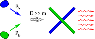
Figure 1: High-energy scattering as a collision of two shock waves.

Indeed, due to the Lorentz contraction the two hadrons shrink into thin “pancakes” which collide producing the final state particles. The main question is the field/particles produced by the collision of two shock waves. On the theoretical side, this question is related to the problem of high-energy effective action and to the ultimate problem of the small-$x$ physics - unitarization of the BFKL pomeron and the Froissart bound in QCD (see book1 ; book2 ). On more practical terms, the immediate result of the scattering of the two shock waves gives the initial conditions for the formation of a quark-gluon plasma studied in the heavy-ion collisions at RHIC (see e.g. the review mclectures ).

The collision of QCD shock waves can be treated using semiclassical methods. The basic idea is that at high energy the density of partons in the transverse plane becomes sufficiently large to give the hard scale necessary for the application of perturbation theory mvmodel ; nncoll . The arguments in favor of this are based on the idea of parton saturation at high energies GLR ; muchu ; mu90 . Consider a single shock wave - hadron, moving at a high speed (in the c.m. frame). The energetic hadron emits more and more gluons and the gluon parton density increases rapidly with energy. This cannot go forever - at some point the recombination of partons balances the emission and partons reach the state of saturation with the charactristic transverse momenta (the “saturation scale”) being $Q_{s}\sim e^{c\eta}$ where $\eta$ is the rapidity mu99 ; mabraun ; iancu02 ; tolpa . Such an energetic shock wave with large density of color charge is called the Color Glass Condensate mvmodel ; CGC .

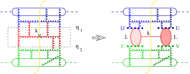
Figure 2: Integration over the central rapidity gluons in a semiclassical approximation.

Within the semiclassical approach, the problem of scatering of two shock waves can be reduced to the solution of classical YM equations with sources being the shock waves nncoll (see also prd99 ). At present, these equations have not been solved. There are two approaches discussed in current literature: numerical simulations krasvenu and expansion in the strength of one of the shock waves kovmu99 ; kop ; wkov .

Note that the collision of a weak and a strong shock waves corresponds to the deep inelastic scattering from a nucleus (while the scattering of two strong shock waves describes a nucleus-nucleus collision). In the present paper I formulate the problem of scattering of shock waves, find the boundary conditions for the double functional integral for the cross section and decribe the expansion in the commutators of two shock waves equivalent to the expansion in strength of one of the waves. The main technical result is the calculation of the second term of this expansion (the first term can be restored from the current literature)

The paper is organized as follows. Sec. 2 is a more formal introduction: I outline the idea of the factorization of the hadron-hadron cross section into the formation of two shock waves and their scattering. In Sec. 3 I discuss the rapidity factorization and define what is a scattering of QCD shock waves. In Sec. 4 I find the Lipatov vertex of the gluon emission and in Sec. 5 reproduce the $k_{T}$-factorization valid in the first order in the commutator expansion (for the $pA$ scattering). In Sec. 6 I obtain the first-order effective action and reproduce the non-linear equation for the small-$x$ evolution of Wilson lines. Sec. 7 outlines the calculation of the second-order classical field in the while the details of the calculation are given in the Appendices A-C. The explicit form of the vertex of gluon emission by two Wilson lines in the shock-wave background is presented in the Appendix D.

II Basic idea: two-step integration over rapidity

In this section I outline how the hadron-hadron collision at high energy is related to the scattering of shock waves. The basic idea of the approach is the two-step integration over rapidity in the double functional integral for the cross section. At first, let us define this integral.

II.1 Double functional integral for the cross section.

A total cross section is a product of an amplitude and a complex conjugate amplitude so the functional intergral for the cross section has double set of fields: to the right of the cut and to the left of the cut. A typical functional integral has the form:

$$\int\!D{\cal A}DA{\cal J}(p_{A}){\cal J}(p_{B})e^{-iS({\cal A})}~{}J(-p_{A})J(-p_{B})~{}e^{iS(A)}$$ (1)

where the currents $J(p_{A})$ and $J(p_{B})$ describe the two colliding particles (say, photons). Throughout the paper, fields to the left of the cut will be represented by the calligraphic letters while those to the right of the cut by usual letters. The boundary conditions are such that the fields $A$ and ${\cal A}$ coincide at $t\rightarrow\infty$, reflecting the summation over the final states implied in the definition of a total cross section. The propagators for such functional integral reproduce the Cutkovsky rules (cf. ref. keld ) :

$$\langle A^{a}_{\mu}(x)A^{b}_{\nu}(y)\rangle=g_{\mu\nu}\delta^{ab}\!\int\!{d^{4}k\over 16\pi^{4}}e^{-ik(x-y)}{-i\over k^{2}+i\epsilon}$$ (2)

$$\langle{\cal A}^{a}_{\mu}(x){\cal A}^{b}_{\nu}(y)\rangle=g_{\mu\nu}\delta^{ab}\!\int\!{d^{4}k\over 16\pi^{4}}e^{-ik(x-y)}{i\over k^{2}-i\epsilon}$$

$$\ \langle{\cal A}^{a}_{\mu}(x)A^{b}_{\nu}(y)\rangle=-g_{\mu\nu}\delta^{ab}\!\int\!{d^{4}k\over 16\pi^{4}}e^{-ik(x-y)}2\pi\delta(k^{2})\theta(k_{0})$$

We are interested in the number of gluons produced per unit rapidity which is given by the average of the creation operator over the final state $\langle a(k_{\perp},\eta)a^{\dagger}(k_{\perp},\eta)\rangle$ (see the discussion in ref. jkmh ). In terms of functional integrals this can be rewritten as

$$n_{g}(k_{\perp},\eta)~{}=~{}\lim_{k^{2}\rightarrow 0}\!\int\!D{\cal A}DA{\cal J}(p_{A}){\cal J}(p_{B})$$ (3)

$$\times~{}e^{-iS({\cal A})}~{}k^{2}{\cal A}^{a}_{i}(k)k^{2}A^{a}_{i}(-k)e^{iS(A)}J(-p_{A})J(-p_{B})$$

Throughout the paper, the sum over the Latin indices $i,j...$ runs over the two transverse components (while the sum over Greek indices runs over the four components as usual). As we shall see below, the Lipatov vertex of gluon emission $R_{\mu}(k)=\lim_{k^{2}\rightarrow 0}A_{\mu}(k)$ is transverse: $k_{\mu}R^{\mu}(k)=)$ so we can replace $A_{i}{\cal A}_{i}$ in Eq. (4) by the sum over all four indices

$$n_{g}(k_{\perp},\eta)~{}=~{}-\lim_{k^{2}\rightarrow 0}\!\int\!D{\cal A}DA{\cal J}(p_{A}){\cal J}(p_{B})$$ (4)

$$\times~{}e^{-iS({\cal A})}~{}k^{2}{\cal A}^{a}_{\mu}(k)k^{2}A^{\mu}(-k)e^{iS(A)}J(-p_{A})J(-p_{B})$$

II.2 Two-step integration.

The integration over the gluon fields in the functional integral (4) will be done in two steps according to the rapidity of the gluons. Let us introduce two rapidities $\eta_{1}$ and $\eta_{2}$ such that $\eta_{A}>\eta_{1}>\eta_{2}>\eta_{B}$. Consider a typical Feynman diagram for the gluon production (4) shown in Fig. 2. At first, we integrate over the fields in the central range of rapidity $\eta_{1}>\eta>\eta_{2}$ and leave the fields with $\eta>\eta_{1}$ and $\eta<\eta_{2}$ in the form of external shock waves. In the semiclassical approximation there is only one gluon emission described by the Lipatov vertex - Fourirer transform of the classical field at the mass shell. The result of the integration is the product of two Lipatov vertices which depend on that “external” fields. It is easy to see that Lipatov vertices depend on these gluon fields through Wilson lines - infinite gauge links ordered along the straight lines collinear to $\eta_{1}$ and $\eta_{2}$. Indeed, in the target frame gluons with rapidities $\eta_{1}>\eta>\eta_{2}$ are very fast so their propagators in the background of “target” gluons reduce to the gauge factor ordered along the straght line classical trajectory.

Thus, in the semiclassical approximation we get (see Fig. 2)

$$n_{g}(k_{\perp};\eta)~{}=~{}\int\!D{\cal A}DAD{\cal B}DB{\cal J}_{A}J_{A}e^{-iS({\cal A})+iS(A)}$$ (5)

$${\cal J}_{B}J_{B}e^{-iS({\cal B})+iS(B)}R(k;V,U,{\cal V},{\cal U})e^{i\int d^{2}z(V_{i}U^{i}-{\cal V}_{i}{\cal U}^{i})}$$

where $R(k;V,U,{\cal V},{\cal U})$ is a product of two Lipatov vertices

$$R(k;V,U,{\cal V},{\cal U})~{}=~{}-R_{\mu}(k;V,U){\cal R}^{\mu}(-k,{\cal V},{\cal U})$$ (6)

The Lipatov vertex $R_{\mu}(k;V,U)=\lim_{k^{2}\rightarrow 0}k^{2}A_{\mu}(k;U,V)$ is an amplitude of the emission of a gluon with momentum $k$ by the two Wilson lines $U$ and $V$. It depends on the gauge, but the product of two Lipatov vertices (6) is gauge-invariant due to the property $k_{\mu}R^{\mu}(k)=0$. Here ${\cal A},A$ are fields with rapidities $\eta>\eta_{1}$ and ${\cal B},B$ with rapidities $\eta<\eta_{2}$. The Wilson lines $V$ and $U$ are made from $A$ and $B$ fields, respectively:

$$V(x_{\perp})=[\infty n_{1}+x_{\perp},-\infty n_{1}+x_{\perp}],$$

$$U=[\infty n_{2}+x_{\perp},-\infty n_{2}+x_{\perp}]$$ (7)

where $n_{1}$ and $n_{2}$ are the unit vectors corresponding to rapidities $\eta_{1}$ and $\eta_{2}$ while $[x,y]$ is a shorthand notation for the straight-line ordered gauge linkconnecting points $x$ and $y$:

$$[x,y]\equiv Pe^{ig\!\int_{0}^{1}\!du(x-y)^{\mu}A_{\mu}(ux+(1-u)y)}$$ (8)

It may seem that the result (5) depends on the artificial “rapidity divides” $\eta_{1}$ and $\eta_{2}$. This dependence should be canceled by the gluon ladder on the top of the Lipatov vertices which is outside the semiclassical approximation. The common belief is that the all the evolution can be attributed to either upper or lower sector: to calculate $n_{g}(k_{\perp},\eta)$, we choose $\eta_{1}$ and $\eta_{2}$ such that both $\alpha_{s}(\eta_{1}-\eta),\alpha_{s}(\eta-\eta_{2})\ll 1$ so the part of the evolution between $\eta_{1}$ and $\eta_{2}$ can be neglected and we can use the semiclassical aproximation for the functional integral (5) over the region of rapidity $\eta_{1}>\eta>\eta_{2}$ (see e.g. the review mclectures ). Eventually, after solving the classical Yang-Mills equations for this functional integral, we can put $\eta_{1}=\eta$ in $V$ and $\eta_{2}=\eta$ in U. The independent evolution in the upper (or lower) sectors leads to the parton saturation so the shock waves $U$ and $V$ have a form of Color Glass Condensate CGC .

To find the Lipatov vertices one needs to solve the classical YM equation with the sources proportional to shock waves $U$ and $V$. As we mentioned, these equations have not been solved yet and there are two approaches discussed in the literature: numerical simulations and expansion in the strength of one of the shock waves. In this paper I develop the second approach in a “symmetric” way as an expansion in commutators $[U,V]$, and calculate the second term of the expansion (the first one can be restored from the literature).

III Rapidity factorization and scattering of the shock waves

III.1 Rapidity factorization

In this section we define the scattering of the shock waves using the rapidity factorization developed in prl ; prd99 . Consider a functional integral for the cross section (1) and take some “rapidity divide” $\eta_{1}$ such that $\eta_{A}>\eta_{1}>\eta_{B}$.

Throughout the paper, we use Sudakov variables

$$k~{}=~{}\alpha p_{1}+\beta p_{2}+k_{\perp}$$ (9)

and the notations

$$x_{\bullet}=p_{1}^{\mu}x_{\mu}=\sqrt{s\over 2}x^{-},~{}~{}~{}~{}x^{-}={1\over\sqrt{2}}(x^{0}-x^{3})$$

$$x_{\ast}=p_{2}^{\mu}x_{\mu}=\sqrt{s\over 2}x^{+},~{}~{}~{}~{}x^{+}={1\over\sqrt{2}}(x^{0}+x^{3})$$ (10)

Here $p_{1}$ and $p_{2}$ are the light-like vectors close to $p_{A}$ and $p_{B}$: $p_{A}=p_{1}+{p_{A}^{2}\over s}p_{2}$, $p_{B}=p_{2}+{p_{B}^{2}\over s}p_{1}$.

Let us integrate first over the fields with the rapidity $\eta>\eta_{1}$. From the viewpont of such particles, the gluons with $\eta<\eta_{1}$ shrink to a shock wave so the result of the integration is presented by Feynman diagrams in the shock-wave background. In the covariant gauge, the shock-wave has the only non-vanishing component $A_{\bullet}$ which is concentrated near $x_{\ast}=0$. A typical Green function $G(x,y)$ at $x_{\ast},y_{\ast}<0$ in the background-Feynman gauge has the form mobzor

$$\langle{\cal A}(x)A(y)\rangle~{}=$$

$$~{}\int dz\delta({2\over s}z_{\ast})(x|{-1\over p^{2}-i\epsilon}\Big{\{}2\alpha g_{\mu\nu}{\cal U}_{z}U_{z}+{4i\over s}(\partial_{\mu}({\cal U}_{z}U_{z})p_{2\nu}$$

$$~{}-\mu\leftrightarrow\nu)-~{}{4p_{2\mu}p_{2\nu}\over\alpha s^{2}}\partial_{\perp}^{2}({\cal U}U)_{z}\Big{\}}(z|{1\over p^{2}+i\epsilon}|y)$$ (11)

where ${\cal U}_{z}=[\infty p_{1}+z_{\perp},-\infty p_{1}+z_{\perp}]$ is made form the left fields ${\cal A}$ while $U_{z}=[\infty p_{1}+z_{\perp},-\infty p_{1}+z_{\perp}]$ is made from $A$’s.

Similarly to the case of the usual functional integral for the amplitude, in order to write down factorization we need to rewrite the shock wave in the temporal gauge $A_{0}=0$. In such gauge the shock-wave background has the form

$${\cal A}_{i}={\cal U}_{i}\theta(-x_{\ast}),~{}~{}{\cal A}_{\bullet}={\cal A}_{\ast}=0,$$

$$A_{i}=U_{i}\theta(-x_{\ast}),~{}~{}A_{\bullet}=A_{\ast}=0$$ (12)

where

$${\cal U}_{i}\equiv{\cal U}{i\over g}\partial_{i}{\cal U}^{\dagger},~{}~{}~{}~{}~{}U_{i}\equiv U{i\over g}\partial_{i}U^{\dagger}$$ (13)

are the pure gauge fields (filling the half-space $x_{\ast}<0$). Note that the choice (12) is different from the choice $A_{i}=U_{i}\theta(x_{\ast})$ adopted in prd99 ; mobzor . The reason is the following: when we calculate the amplitude, it is natural to use the redundant gauge rotation to get rid of the field at $t=-\infty$ (althougth the choice $t=\infty$ is equally possible). On the contrary, for a double functional integral of the form (1), we have two independent integrations at $t=-\infty$ and it is impossible to eliminate both of them. We can however gauge away fields at $t=\infty$ because of the boundary condition $A={\cal A}|_{t=\infty}$. (Stricltly speaking, we cannot gauge away all the fields; what we can do is to forbid a pure gauge fields $t=\infty$ which is enough for our purposes since it puts forward the choice (12) over the choice $U_{i}\theta(x_{\ast})$).

The Green functions in the background (12) differ from those of (11) by a simple gauge rotation. Their explicit form is presented in the Appendix A.1.

The generating functional for the Green functions in the Eq. (12) background is obtained by the generalization of the generating functional of mobzor to the case of a double functional integral:

$$\int\!D{\cal A}DA{\cal J}(p_{A})J(-p_{A})e^{-iS({\cal A})+i\!\int\!d^{2}z_{\perp}(\infty,{\cal F}_{\ast i},\infty)^{a}_{z}{\cal U}^{ai}_{z}}$$

$$~{}e^{iS(A)-i\!\int\!d^{2}z_{\perp}(\infty,F_{\ast i},\infty)^{a}_{z}U^{ai}_{z}}$$ (14)

where the Wilson-line operator

$$(\infty,{\cal F}_{\mu i},\infty)^{a}\equiv$$ (15)

$$2{\rm tr}~{}t^{a}\!\int_{-\infty}^{\infty}\!\!du~{}[\infty p_{2},up_{2}]_{z}{\cal F}_{\mu i}(up_{2}+z_{\perp})[up_{2},-\infty p_{2}]_{z},$$

is made from the “left” fields ${\cal A}_{\mu}$ and the operator

$$(\infty,F_{\mu i},\infty)^{a}\equiv$$

$$2{\rm tr}~{}t^{a}\!\int_{-\infty}^{\infty}\!\!du~{}[\infty p_{2},up_{2}]_{z}F_{\mu i}(up_{2}+z_{\perp})[up_{2},-\infty p_{2}]_{z}$$

from the “right” fields $A_{\mu}$.

It is easy to see that the functional integral (14) generates Green functions in the Eq. (12) background. Indeed, let us choose the gauge $A_{\ast}={\cal A}_{\ast}=0$ for simplicity. In this gauge $(\infty,{\cal F}_{\ast i},\infty)^{a}={\cal A}_{i}(\infty p_{2}+z_{\perp})-{\cal A}_{i}(-\infty p_{2}+z_{\perp})$ and $(\infty,F_{\ast i},\infty)^{a}=A_{i}(\infty p_{2}+z_{\perp})-A_{i}(-\infty p_{2}+z_{\perp})$. so the functional integral (14) takes the form

$$\int\!D{\cal A}DA{\cal J}(p_{A})J(-p_{A})$$ (16)

$$\times~{}e^{-iS({\cal A})+i\!\int\!d^{2}z_{\perp}({\cal A}_{i}(\infty p_{2}+z_{\perp})-{\cal A}_{i}(-\infty p_{2}+z_{\perp}))^{a}{\cal U}^{ai}}$$

$$\times~{}e^{iS(A)-i\!\int\!d^{2}z_{\perp}(A_{i}(\infty p_{2}+z_{\perp})-A_{i}(-\infty p_{2}+z_{\perp}))^{a}U^{ai}}$$

Let us now shift the fields $A_{i}\rightarrow A_{i}+\bar{A}_{i}$ and ${\cal A}_{i}\rightarrow{\cal A}_{i}+\bar{{\cal A}}_{i}$ where $\bar{A}_{i}=U_{i}\theta(-x_{\ast})$ and $\bar{\cal A}_{i}={\cal U}_{i}\theta(-x_{\ast})$. The only non-zero components of the classical field strength in our case are $F_{\bullet i}=-U_{i}\delta({2\over s}x_{\ast})$ so we get (for the “right” sector)

$$S(A+\bar{A})~{}=~{}{2\over s}\!\int d^{4}zD^{i}\bar{F}_{i\bullet}A^{\ast}-{2\over s}\int\!d^{2}z_{\perp}dz_{\bullet}$$

$$\times~{}\left.A^{i}\bar{F}_{\bullet i}\right|^{x_{\ast}=\infty}_{x_{\ast}=-\infty}+{1\over 2}A^{\mu}(\bar{D}^{2}g_{\mu\nu}-2i\bar{\cal F}_{\mu\nu})A^{\nu}+...$$ (17)

In the $A_{\ast}=0$ gauge the first term in the r.h.s. of Eq. (17) vanishes while the second term cancels with the corresponding contribution $\sim-(A_{i}(\infty p_{2}+z_{\perp})-A_{i}(-\infty p_{2}+z_{\perp}))^{a}U^{ai}$ coming from the source in Eq. (14). Similar cancellation occurs in the left sector so we get

$$\int\!D{\cal A}DA{\cal J}(p_{A})J(-p_{A})$$ (18)

$$\times~{}e^{-iS({\cal A})+i\!\int\!d^{2}z_{\perp}[{\cal A}_{i}(\infty p_{2}+z_{\perp})-{\cal A}_{i}(-\infty p_{2}+z_{\perp})]^{a}{\cal U}^{ai}_{z}}$$

$$\times~{}e^{iS(A)-i\!\int\!d^{2}z_{\perp}[A_{i}(\infty p_{2}+z_{\perp})-A_{i}(-\infty p_{2}+z_{\perp})]^{a}U^{ai}_{z}}$$

$$=~{}\int\!D{\cal A}DA{\cal J}(p_{A})J(-p_{A})$$

$$\times~{}e^{-{i\over 2}\!\int\!d^{2}z{\cal A}^{\mu}(\bar{\cal D}^{2}g_{\mu}\nu-2i\bar{\cal F}_{\mu\nu}){\cal A}^{\nu}}e^{{i\over 2}\!\int\!d^{2}zA^{\mu}(\bar{D}^{2}g_{\mu}\nu-2i\bar{F}_{\mu\nu})A^{\nu}}$$

which gives the Green functions in the Eq. (12) background.

To complete the factorization formula one needs to integrate over the remaining fields with rapidities $\eta<\eta_{1}$:

$$\int\!D{\cal A}DA{\cal J}(p_{A}){\cal J}(p_{B})e^{-iS({\cal A})}~{}e^{iS(A)}J(-p_{A})J(-p_{B})$$

$$=~{}\int\!D{\cal A}DA{\cal J}(p_{A})J(-p_{A})\int\!D{\cal B}DB{\cal J}(p_{B})J(-p_{B})$$

$$\times~{}e^{-iS({\cal A})-iS({\cal B})+i\!\int\!d^{2}z_{\perp}(\infty,{\cal F}_{\mu i},\infty)^{a}_{z}(\infty,{\cal G}_{\nu i},\infty)^{a}_{z}e_{1}^{\mu}e_{1}^{\nu}}$$

$$\times~{}e^{iS(A)+iS(B)-i\!\int\!d^{2}z_{\perp}(\infty,F_{\mu i},\infty)^{a}_{z}(\infty,G_{\nu i},\infty)^{a}_{z}e_{1}^{\mu}e_{1}^{\nu}}$$ (19)

As discussed in prl ; prd99 ; mobzor ; baba03 , the slope of Wilson lines is determined by the “rapidity divide” vector $e_{\eta_{1}}=p_{1}+e^{-\eta_{1}}p_{2}$. (From the wiewpoint of $A$ fields, the slope $e_{1}$ can be replaced by $p_{2}$ with power accuracy so we recover the generating functional (14) with $U_{i}=(\infty,G_{\ast i},\infty)$, ${\cal U}_{i}=(\infty,{\cal G}_{\ast i},\infty)$).

Applying the factorization formula (III.1) two times one gets:

$$-\lim_{k^{2}\rightarrow 0}\!\int\!D{\cal A}DA{\cal J}(p_{A}){\cal J}(p_{B})$$ (20)

$$\times~{}e^{-iS({\cal A})}~{}k^{2}{\cal A}^{a\mu}(k)k^{2}A^{a}_{\mu}(-k)e^{iS(A)}J(-p_{A})J(-p_{B})$$

$$=~{}-\int\!D{\cal A}DA{\cal J}(p_{A})J(-p_{A})e^{-iS({\cal A})+iS(A)}$$

$$\!\int\!D{\cal B}DB{\cal J}(p_{B})J(-p_{B})e^{-iS({\cal B})+iS(B)}$$

$$\times~{}\int\!D{\cal C}DC\lim_{p^{2}\rightarrow 0}p^{2}{\cal C}^{a\mu}(p)p^{2}C^{a}_{\mu}(-p)\exp\Big{[}-iS({\cal C})$$

$$+~{}iS(C)+\!\int\!d^{2}z_{\perp}\Big{\{}e_{1}^{\mu}e_{1}^{\nu}\Big{(}[\infty,{\cal A}_{\mu i},\infty]^{a}_{z}[\infty,{\cal C}_{\nu i},\infty]^{a}_{z}$$

$$-~{}[\infty,A_{\mu i},\infty]^{a}_{z}[\infty,C_{\nu i},\infty]^{a}_{z}\Big{)}+e_{2}^{\mu}e_{2}^{\nu}\Big{(}(\infty,{\cal C}_{\mu i},\infty)^{a}_{z}$$

$$\times~{}(\infty,{\cal B}_{\nu i},\infty)^{a}_{z}-(\infty,C_{\mu i},\infty)^{a}_{z}(\infty,B_{\nu i},\infty)^{a}_{z}\Big{)}\Big{\}}\Big{]}$$

where the slope is $e_{1}=p_{1}+e^{-\eta_{1}}p_{2}$ for the $[...]$ Wilson lines and $e_{2}=p_{1}+e^{-\eta_{2}}p_{2}$ for the $(...)$ ones.

The functional integral over the central range of rapidity $\eta_{1}>\eta>\eta_{2}$ is determined by scattering of shock two shock waves:

$$-\!\int\!\!D{\cal C}DC\lim_{k^{2}\rightarrow 0}k^{2}{\cal C}^{a\mu}(k)k^{2}C^{a}_{\mu}(-k)\exp\Big{[}iS(C)-iS({\cal C})$$

$$\!\int\!d^{2}z_{\perp}\Big{\{}e_{1}^{\mu}\Big{(}{\cal V}^{ai}_{z}[\infty,{\cal C}_{\mu i},\infty]^{a}_{z}-V^{ai}_{z}[\infty,C_{\nu i},\infty]^{a}_{z}\Big{)}$$

$$+~{}\Big{(}{\cal U}^{ai}_{z}(\infty,{\cal C}_{\mu i},\infty)^{a}_{z}-U^{ai}_{z}(\infty,C_{\mu i},\infty)^{a}_{z}\Big{)}e_{2}^{\mu}\Big{\}}\Big{]}$$ (21)

where ${\cal V}_{i}=e_{1}^{\mu}[\infty,{\cal A}_{\mu i},\infty]$, $V_{i}=e_{1}^{\mu}[\infty,A_{\mu i},\infty]$, ${\cal U}_{i}=e_{2}^{\mu}(\infty,{\cal B}_{\mu i},\infty)$, and $U_{i}=e_{2}^{\mu}(\infty,B_{\mu i},\infty)$ are the pure-gauge “external” fields (to be integrated over later). With a power accuracy $O(m^{2}/s)$, we can replace $e_{1}$ by $p_{1}$ and $e_{2}$ by $p_{2}$ :

$$-\!\int\!\!D{\cal C}DC\lim_{k^{2}\rightarrow 0}k^{2}{\cal C}^{a\mu}(k)k^{2}C^{a}_{\mu}(-k)\exp\Big{\{}iS(C)-iS({\cal C})$$

$$+~{}i\!\int\!d^{2}z_{\perp}\Big{(}{\cal V}^{ai}_{z}[\infty,{\cal C}_{\bullet i},\infty]^{a}_{z}+(\infty,{\cal C}_{\ast i},\infty)^{a}_{z}{\cal U}^{ai}_{z}$$

$$\hskip 14.22636pt-~{}V^{ai}_{z}[\infty,C_{\bullet i},\infty]^{a}_{z}-(\infty,C_{\ast i},\infty)^{a}_{z}U^{ai}_{z}\Big{)}\Big{\}}$$ (22)

The saddle point of the functional integral (22) is determined by the classical equations

$${\delta\over\delta C_{\mu}^{a}}\Big{\{}S(C)-i\!\int\!d^{2}z_{\perp}\Big{(}V^{ai}_{z}[\infty,C_{\bullet i},\infty]^{a}_{z}$$

$$\hskip 56.9055pt+~{}(\infty,C_{\ast i},\infty)^{a}_{z}U^{ai}_{z}\Big{)}\Big{\}}~{}=~{}0$$

$${\delta\over\delta{\cal C}_{\mu}^{a}}\Big{\{}S({\cal C})-i\!\int\!d^{2}z_{\perp}\Big{(}{\cal V}^{ai}_{z}[\infty,{\cal C}_{\bullet i},\infty]^{a}_{z}$$

$$\hskip 56.9055pt+~{}(\infty,{\cal C}_{\ast i},\infty)^{a}_{z}{\cal U}^{ai}_{z}\Big{)}~{}=~{}0$$

(23)

At present it is not known how to solve this equations (for the numerical solution see krasvenu ). In the next section we will develop a “perturbation theory” in powers of the parameter $[U,V]\sim g^{2}[U_{i},V_{j}]\sim g^{2}[{\cal U}_{i},{\cal V}_{j}]$. Note that the conventional perturbation theory corresponds to the case when $U_{i},V_{i}\sim 1$ while the semiclassical QCD is relevant when the fields are large ($U_{i}$ and/or $V_{i}\sim{1\over g}$).

III.2 Expansion in commutators of Wilson lines

The particle production due to scattering of the two shock waves in QCD (see Fig. 3)

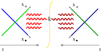
Figure 3: Particle production due to the scattering of the two shock waves.

is determined by the functional integral (22) (hereafter we switch back to the usual notation $A_{\mu}$ for the integration variable and $F_{\mu\nu}$ for the field strength)

$$R(p;U,V,{\cal U},{\cal V})~{}=~{}-\lim_{k^{2}\rightarrow 0}\int\!\!D{\cal A}DA~{}k^{2}{\cal A}^{a\mu}(k)$$

$$\times~{}k^{2}A^{a}_{\mu}(-k)~{}\exp\Big{\{}-iS({\cal A})+i\!\int\!d^{2}z_{\perp}\Big{(}{\cal V}^{ai}_{z}[\infty,{\cal F}_{\ast i},\infty]^{a}_{z}$$

$$+~{}(\infty,{\cal F}_{\ast i},\infty)^{a}_{z}{\cal U}^{ai}_{z}\Big{)}+iS(A)-i\!\int\!d^{2}z_{\perp}\Big{(}V^{ai}_{z}$$

$$\hskip 36.98857pt\times~{}[\infty,F_{\ast i},\infty]^{a}_{z}+(\infty,F_{\ast i},\infty)^{a}_{z}U^{ai}_{z}\Big{\}}$$ (24)

Taken separately, the source $U_{i}$ creates a shock wave $U_{i}\theta(-x_{\ast})$ and $V_{i}$ creates $V_{i}\theta(-x_{\bullet})$ (to the left of the cut, ${\cal U}_{i}$ generates the classical field ${\cal U}_{i}\theta(-x_{\ast})$ and ${\cal V}_{i}$ generates ${\cal V}_{i}\theta(-x_{\bullet})$ ). In QED, the two sources $U_{i}$ and $V_{i}$ do not interact so the sum of the two shock waves

$$\bar{\cal A}_{i}^{(0)}={\cal U}_{i}\theta(-x_{\ast})+{\cal V}_{i}\theta(-x_{\bullet}),~{}~{}~{}\bar{\cal A}_{\bullet}^{(0)}=\bar{\cal A}_{\ast}^{(0)}=0$$

$$\bar{A}_{i}^{(0)}=U_{i}\theta(-x_{\ast})+V_{i}\theta(-x_{\bullet}),~{}~{}~{}\bar{A}_{\bullet}^{(0)}=\bar{A}_{\ast}^{(0)}=0$$ (25)

is a classical solution to the set of equations (23). In QCD, the interaction between these two sources is described by the commutator $g[U_{i},V_{k}]$ (the coupling constant $g$ corresponds to the three-gluon vertex). It is natural to take the trial configuration in the form of a sum of the two shock waves and expand the “deviation” of the full QCD solution from the QED-type ansatz (25) in powers of commutators $[U,V]$. To carry this out, one shifts $A\rightarrow A+\bar{A}_{i}^{(0)}$, ${\cal A}\rightarrow{\cal A}+\bar{\cal A}_{i}^{(0)}$ in the functional integral (24) and obtains

$$R(k;U,V,{\cal U},{\cal V})~{}=~{}-\int\!D{\cal A}DA~{}\lim_{k^{2}\rightarrow 0}k^{2}{\cal A}^{a\mu}(k)$$

$$\times~{}k^{2}A^{a}_{\mu}(-k)\exp\Big{\{}i\!\int\!d^{4}z\Big{(}-({1\over 2}{\cal A}^{\mu}\bar{\cal D}_{\mu\nu}{\cal A}^{\nu}$$

$$+~{}{1\over 2}A^{\mu}\bar{D}_{\mu\nu}A^{\nu}-{\cal T}^{\mu}{\cal A}_{\mu}+T^{\mu}A_{\mu}\Big{)}\Big{\}}~{},$$ (26)

Here $D_{\mu\nu}=D^{2}(\bar{A})g_{\mu\nu}-2i\bar{F}_{\mu\nu}$ (${\cal D}_{\mu\nu}=D^{2}(\bar{\cal A})g_{\mu\nu}-2i\bar{\cal F}_{\mu\nu}$) is the inverse propagator in the background-Feynman gauge and $T_{\mu}({\cal T}_{\mu}$ is the linear term for the trial configuration (25)

$$T_{\mu}~{}=~{}-D^{k}F_{\mu k}\theta(-z_{\ast})\theta(-z_{\bullet})$$ (27)

$$+~{}ig[U_{i},V^{i}]\Big{(}p_{1\mu}\theta(z_{\ast})\delta(z_{\bullet})-p_{2\mu}\theta(z_{\bullet})\delta(z_{\ast})\Big{)}$$

$${\cal T}_{\mu}~{}=~{}-D^{k}{\cal F}_{\mu k}\theta(-z_{\ast})\theta(-z_{\bullet})$$

$$+~{}ig[{\cal U}_{i},{\cal V}^{i}]\Big{(}p_{1\mu}\theta(z_{\ast})\delta(z_{\bullet})-p_{2\mu}\theta(z_{\bullet})\delta(z_{\ast})\Big{)}$$

where $\bar{F}_{ik}=-ig[U_{i},V_{k}]-i\leftrightarrow k$ (and $\bar{\cal F}_{ik}=-ig[{\cal U}_{i},{\cal V}_{k}]-i\leftrightarrow k$).

Expanding in powers of $T$(${\cal T}$) in the functional integral (26) one gets the set of Feynman diagrams in the external fields (25) with the sources (27). The parameter of the expansion is $g^{2}[U_{i},V_{j}]$ ($\sim[U,V]$, see Eq. (13)).

IV Classical fields and Lipatov vertex in the first order in $[U,V]$

The general formulas for the classical solution in the first order in $[U,V]$ ($[{\cal U},{\cal V}]$) have the form

$$\bar{A}^{(1)a}_{\mu}(x) = i\!\int\!d^{4}z\Big{(}\langle A^{a}_{\mu}(x)A^{b\nu}(z)\rangle_{\bar{A},\bar{\cal A}}T^{b}_{\nu}(z)$$

$$- ~{}~{}~{}~{}~{}\langle A^{a}_{\mu}(x){\cal A}^{b\nu}(z)\rangle_{\bar{A},\bar{\cal A}}{\cal T}^{b}_{\nu}(z)\Big{)}$$

$$\bar{\cal A}^{(1)a}_{\mu}(x) = i\!\int\!d^{4}z\Big{(}\langle{\cal A}^{a}_{\mu}(x)A^{b\nu}(z)\rangle_{\bar{A},\bar{\cal A}}T^{b}_{\nu}(z)$$ (28)

$$- ~{}~{}~{}~{}~{}\langle{\cal A}^{a}_{\mu}(x){\cal A}^{b\nu}(z)\rangle_{\bar{A},\bar{\cal A}}{\cal T}^{b}_{\nu}(z)\Big{)}$$

The Green functions in the background of the Eq. (25) field can be approximated by cluster expansion

$$\langle A_{\mu}(x)A^{\nu}(z)\rangle_{\bar{A},\bar{\cal A}}$$

$$=~{}\langle A_{\mu}(x)A^{\nu}(z)\rangle_{U,{\cal U}}+\langle A_{\mu}(x)A^{\nu}(z)\rangle_{V,{\cal V}}$$

$$-~{}\langle A_{\mu}(x)A^{\nu}(z)\rangle_{0}+O([U,V],[{\cal U},{\cal V}])$$ (29)

(and similarly for other sectors) where $\langle A_{\mu}(x)A^{\nu}(z)\rangle_{0}$ are the perturbative propagators (2) and the propagators in the background of one shock wave are given in the Appendix A.1. As a first step we shall discuss the behavior of classical fields at the $t=-\infty$ boundary.

IV.1 Pure gauge fields at $t=-\infty$

Note that while each of the field $U_{i}$ and $V_{i}$ satisfies the boundary condition $A_{i}(t\rightarrow-\infty)$ = pure gauge, their sum (25) does not. I will demonstrate now that the correction (28) restores this property so $\bar{A}^{(0)}+\bar{A}^{(1)}$ is a pure gauge (up to $[U,V]^{2}$ terms).

We need to prove that $\bar{D}_{\mu}\bar{A}^{(1)}_{\nu}-\mu\leftrightarrow\nu$ cancels $\bar{F}_{ik}=-ig([U_{i},V_{k}]-i\leftrightarrow k)$ as $t\rightarrow-\infty$ . First, note that the contribution from terms $[U_{i},V^{i}]$ in $T$ (and $[{\cal U}_{i},{\cal V}^{i}]$ in ${\cal T}$) vanishes at $t\rightarrow-\infty$ since these sources are located at $t\geq 0$. Also, it is easy to see that the Green functions $\langle{\cal A}_{\mu}(x)A^{\nu}(y)\rangle$ interpolating between sectors also vanish at this limit (see the explicit expressions in the Appendix A). The only nonzero contribution to $A^{(1)}_{\nu}$ at $t=-\infty$ has the form

$$A^{(1)}_{i}(x)=g\!\int\!d\alpha d\beta d^{2}z_{\perp}{e^{-i\alpha x_{\bullet}-i\beta x_{\ast}}\over(\alpha-i\epsilon)(\beta-i\epsilon)}(U_{x}U^{\dagger}_{z}+V_{x}V^{\dagger}_{z}$$

$$-~{}1)^{ab}(x_{\perp}|{p^{k}\over\alpha\beta s-p_{\perp}^{2}+i\epsilon}|0,z_{\perp})([U_{i},V_{k}]_{z}-i\leftrightarrow k)$$

$$=~{}g(x_{\perp}|U{p^{k}\over p_{\perp}^{2}}U^{\dagger}+V{p^{k}\over p_{\perp}^{2}}V^{\dagger}-{p^{k}\over p_{\perp}^{2}}|[U_{i},V_{k}]-i\leftrightarrow k)$$ (30)

Throughout the paper, we use the notations

$$(x_{\perp}|...|f)\equiv\int d^{2}z_{\perp}(x_{\perp}|...|z_{\perp})f(z_{\perp})$$

$$(x|...|0,f)\equiv\int d^{2}z_{\perp}(x|...|0,z_{\perp})f(z_{\perp})$$ (31)

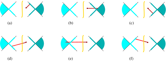
Figure 4: Classical field in the first order. The shaded area represents the linear term (27).

From Eq. (30) we obtain

$$D_{i}A^{a(1)}_{j}-i\leftrightarrow j$$ (32)

$$=~{}g(x_{\perp}|U{p_{i}p^{k}\over p_{\perp}^{2}}U^{\dagger}+V{p_{i}p^{k}\over p_{\perp}^{2}}V^{\dagger}-{p_{i}p^{k}\over p_{\perp}^{2}}|^{ab}\bar{F}^{b}_{jk})-i\leftrightarrow j$$

Because $\bar{F}_{jk}\sim\epsilon_{ik}$ in two dimensions $p_{i}p^{k}~{}\bar{F}_{jk}-i\leftrightarrow j=p_{\perp}^{2}\bar{F}_{ij}$ and therefore

$$D_{i}A^{(1)}_{j}-i\leftrightarrow j~{}=~{}g\bar{F}_{ij}$$ (33)

so the sum $\bar{A}_{0}+\bar{A}_{1}$ is a pure gauge (up to $[U,V]^{2}$ terms).

It can be demonstrated that if we use background-Feynman gauge for calculations in further orders in $[U,V]$ parameter we obtain a pure gauge field $W_{i}=U_{i}+V_{i}+gE_{i}$ where $(i\partial_{i}+g[U_{i}+V_{i},)E^{i}=0$. Similarly, in the left sector the pure gauge field at $t=-\infty$ will be ${\cal W}_{i}={\cal U}_{i}+{\cal V}_{i}+g{\cal E}_{i}$ with ${\cal E}$ satisfying the equation $(i\partial_{i}+g[{\cal U}_{i}+{\cal V}_{i},){\cal E}^{i}=0$.

In the lowest order in $[U,V]$ we get (cf. ref. prd99 ; mobzor )

$$E_{i}=(x_{\perp}|U{p^{k}\over p_{\perp}^{2}}U^{\dagger}+V{p^{k}\over p_{\perp}^{2}}V^{\dagger}-{p^{k}\over p_{\perp}^{2}}|[U_{i},V_{k}]-i\leftrightarrow k)$$

$${\cal E}_{i}=(x_{\perp}|{\cal U}{p^{k}\over p_{\perp}^{2}}{\cal U}^{\dagger}+{\cal V}{p^{k}\over p_{\perp}^{2}}{\cal V}^{\dagger}-{p^{k}\over p_{\perp}^{2}}|[{\cal U}_{i},{\cal V}_{k}]-i\leftrightarrow k)$$ (34)

The explicit expression for the correction $E_{i}$ in the second order in $[U,V]$ is obtained in the Appendix B.

IV.2 Gluon fields in the first order

To find the amplitude of particle production due to the scattering of the two shock waves we should study the behavior of gluon fields at $t\rightarrow\infty$. The general expression for the gluon fields up to the first order in $[U,V]$ is given in Eq. (28) and the corresponding diagrams are shown in Fig. 4.

Let us find the gauge field $A_{\bullet}^{(1)}$ in the $x_{\ast},x_{\bullet}>0$ sector of the space (we use the background-Feynman gauge). This field is a sum two terms: due to $[U_{i},V^{i}]$ and due to $[U_{i},V_{k}]-i\leftrightarrow k$. The $[U_{i},V^{i}]$ term comes from the diagrams shown in Fig. 4c and 4d. Since the Green functions in the shock-wave background in the forward cone $x_{\ast},x_{\bullet},y_{\ast},y_{\bullet}\geq 0$ are just the bare propagators (2), we obtain

$$A_{\bullet}(x) = g(x|{(\alpha+i\epsilon)^{-1}\over p^{2}+i\epsilon}|0,[U_{i},V^{i}])$$ (35)

$$+ ig(x|{\theta(-\alpha)\over\alpha}2\pi\delta(p^{2})|0,[{\cal U}_{i},{\cal V}^{i}])$$

where the first term in the r.h.s. of this equation comes from the diagram in Fig. 4c and the second one from Fig. 4d. The factor $1/\alpha$ in the denominators comes from the integration over the final point $z_{\bullet}$ from $0$ to $\infty$ in the expression for the $[U_{i},V^{i}]$ part of the linear term (27).

The term $\sim[U_{i},V_{k}]$ is obtained by integration of the Green functions (A1)-(A3) in the diagrams in Fig.4b and Fig.4e over the final points $z_{\ast},z_{\perp}<0$:

$$A_{\bullet}(x)~{}=~{}$$ (36)

$$g{s^{2}\over 2}\!\int\!{d\alpha d\beta d\beta^{\prime}\over 8\pi^{3}}{e^{-i\alpha x_{\bullet}-i\beta x_{\ast}}\over(\alpha-i\epsilon)(\beta^{\prime}-i\epsilon)}\Big{\{}(x_{\perp}|{1\over\alpha\beta s-p_{\perp}^{2}+i\epsilon}\partial_{i}U{p^{k}\over\alpha\beta^{\prime}s-p_{\perp}^{2}+i\epsilon}U^{\dagger}|^{ab}0,[U_{i},V_{k}]-i\leftrightarrow k)$$

$$+~{}(x_{\perp}|\theta(-\alpha)2\pi\delta(\alpha\beta s-p_{\perp}^{2})\partial_{i}U{p^{k}\over\alpha\beta^{\prime}s-p_{\perp}^{2}-i\epsilon}U^{\dagger}|^{ab}0,[{\cal U}_{i},{\cal V}_{k}]-i\leftrightarrow k)$$

$$=~{}g(x|{(\alpha-i\epsilon)^{-1}\over p^{2}+i\epsilon}|0,[U_{i},E^{i}])+g(x|{\theta(-\alpha)\over\alpha}2\pi\delta(p^{2})|0,[{\cal U}_{i},{\cal E}^{i}])$$

where we have used the notations (34) for brevity. The field $A_{\bullet}^{1)}$ is the sum of Eqs. (35) and (36). The field $A_{\ast}^{1)}$ is obtained from $A_{\bullet}^{1)}$ by the replacements $x_{\ast}\leftrightarrow x_{\bullet}$ and $U\leftrightarrow V$.

Finally, let us calculate the field $A_{i}^{(1)}$ coming from the diagrams in Figs. 4b and 4e. Using the cluster expansion (29) for the Green functions ${1\over P^{2}}P_{k}$ and the set of the propagators from Appendix A.1, we obtain

$$A_{i}(x)~{}=~{}$$ (37)

$$g\!\int\!{d\alpha d\beta\over 4\pi^{2}}e^{-i\alpha x_{\bullet}-i\beta x_{\ast}}\Bigg{\{}(x_{\perp}|{1\over\alpha\beta s-p_{\perp}^{2}+i\epsilon}\Bigg{[}is\!\int\!{d\beta^{\prime}\over 2\pi(\beta^{\prime}-i\epsilon)}U{p^{k}\over\alpha\beta^{\prime}s-p_{\perp}^{2}+i\epsilon}U^{\dagger}$$

$$+is\!\int\!{d\alpha^{\prime}\over 2\pi(\alpha^{\prime}-i\epsilon)}V{p^{k}\over\alpha^{\prime}\beta s-p_{\perp}^{2}+i\epsilon}V^{\dagger}-{1\over(\alpha-i\epsilon)(\beta-i\epsilon)}{p^{k}\over\alpha\beta s-p_{\perp}^{2}+i\epsilon}\Bigg{]}^{ab}|0,[U_{i},V_{k}]-i\leftrightarrow k)$$

$$+i(x_{\perp}|\theta(-\alpha)2\pi\delta(\alpha\beta s-p_{\perp}^{2})\Bigg{[}is\!\int\!{d\beta^{\prime}\over 2\pi(\beta^{\prime}-i\epsilon)}{\cal U}{p^{k}\over\alpha\beta^{\prime}s-p_{\perp}^{2}+i\epsilon}{\cal U}^{\dagger}$$

$$+is\!\int\!{d\alpha^{\prime}\over 2\pi(\alpha^{\prime}-i\epsilon)}{\cal V}{p^{k}\over\alpha^{\prime}\beta s-p_{\perp}^{2}+i\epsilon}{\cal V}^{\dagger}-{1\over(\alpha-i\epsilon)(\beta-i\epsilon)}{p^{k}\over\alpha\beta s-p_{\perp}^{2}+i\epsilon}\Bigg{]}^{ab}|0,[{\cal U}_{i},{\cal V}_{k}]-i\leftrightarrow k)\Bigg{\}}$$

$$=~{}2g(x|{1\over p^{2}+i\epsilon}|0,E_{i})+2ig(x|\theta(-p_{0})\delta(p^{2})|0,{\cal E}_{i})$$

The left-sector fileds ${\cal A}_{\mu}$ are obtained by trivial replacements.

Let us present the the final set of gauge fields (at $x_{\ast},x_{\bullet}>0$)

$$A_{\bullet}^{(1)}~{}=~{}g(x|{(\alpha+i\epsilon)^{-1}\over p^{2}+i\epsilon}|0,[U_{i},V^{i}])+2g(x|{(\alpha-i\epsilon)^{-1}\over p^{2}+i\epsilon}|0,[U_{i},E^{i}])+ig(x|{\theta(-\alpha)\over\alpha}2\pi\delta(p^{2})|0,[{\cal U}_{i},{\cal V}_{i}+2{\cal E}^{i}])$$

$$A_{\ast}^{(1)}~{}=~{}-g(x|{(\beta+i\epsilon)^{-1}\over p^{2}+i\epsilon}|0,[U_{i},V^{i}])+2g(x|{(\beta-i\epsilon)^{-1}\over p^{2}+i\epsilon}|0,[V_{i},E^{i}])+ig(x|{\theta(-\beta)\over\beta}2\pi\delta(p^{2})|0,[{\cal V}_{i},{\cal U}_{i}+2{\cal E}^{i}])$$

$$A_{i}^{(1)}~{}=~{}2g(x|{1\over p^{2}+i\epsilon}|0,E_{i})+2ig(x|\theta(-p_{0})2\pi\delta(p^{2})|0,{\cal E}_{i})$$

$${\cal A}_{\bullet}^{(1)}~{}=~{}g(x|{(\alpha+i\epsilon)^{-1}\over p^{2}-i\epsilon}|0,[{\cal U}_{i},{\cal V}^{i}])+2g(x|{(\alpha-i\epsilon)^{-1}\over p^{2}-i\epsilon}|0,[{\cal U}_{i},{\cal E}^{i}])-ig(x|{\theta(\alpha)\over\alpha}2\pi\delta(p^{2})|0,[U_{i},V_{i}+2E^{i}])$$

$${\cal A}_{\ast}^{(1)}~{}=~{}-g(x|{(\beta+i\epsilon)^{-1}\over p^{2}-i\epsilon}|0,[{\cal U}_{i},{\cal V}^{i}])+2g(x|{(\beta-i\epsilon)^{-1}\over p^{2}-i\epsilon}|0,[{\cal V}_{i},{\cal E}^{i}])-ig(x|{\theta(\beta)\over\beta}2\pi\delta(p^{2})|0,[V_{i},U_{i}+2E^{i}])$$

$${\cal A}_{i}^{(1)}~{}=~{}2g(x|{1\over p^{2}-i\epsilon}|0,{\cal E}_{i})-2ig(x|\theta(p_{0})2\pi\delta(p^{2})|0,E_{i})$$ (38)

where $E$ and ${\cal E}$ are given by expressions (34). It is easy to see that the fields (38) satisfy the boundary conditions ${\cal A}(x_{\ast}+x_{\bullet}\rightarrow\infty)=A(x_{\ast}+x_{\bullet}\rightarrow\infty)$. The fields $A_{\mu}$ for the right sector only (with ${\cal U}_{i}={\cal V}_{i}=0$) coincide with refs. prd99 ; mobzor

IV.3 Particle production and Lipatov vertex

The particle production is determined by the behavior of the fields at $t=\infty$ described by the Lipatov vertex

$$R_{\mu}(k_{\perp},\eta)=\lim_{k^{2}\rightarrow 0}k^{2}A_{\mu}(k)$$ (39)

$$=~{}2gE_{\mu}+{2p_{2\mu}\over\alpha s}g[U_{i},V^{i}+2E^{i}]+{2p_{1\mu}\over\beta s}g[V_{i},U^{i}+2E^{i}]$$

$${\cal R}_{\mu}(k_{\perp},\eta)=\lim_{k^{2}\rightarrow 0}k^{2}{\cal A}_{\mu}(k)$$

$$=~{}2g{\cal E}_{\mu}+{2p_{2\mu}\over\alpha s}g[{\cal U}_{i},{\cal V}^{i}+2{\cal E}^{i}]+{2p_{1\mu}\over\beta s}g[{\cal V}_{i},{\cal U}^{i}+2{\cal E}^{i}]$$

The vertex (39) is transverse: $k_{\mu}R^{\mu}(k)~{}=~{}k_{i}E^{i}+[U_{i}+V_{i},E^{i}]=0$ due to our choice of $E_{i}$ such that $(i\partial_{i}+[U_{i}+V_{i},)E^{i}=0$. Similarly, $k^{\mu}{\cal R}_{\mu}(k)=0$

It is worth noting that in the case of two weak sources $U_{i}\sim(k-k^{\prime})_{i}$ and $V_{i}\sim k^{\prime}_{i}$ the vertex (39) reduces to

$$R_{\mu}(k;k^{\prime})~{}\sim~{}$$

$${2\over s}(k^{\prime},k-k^{\prime})_{\perp}\Big{(}{p_{1}\over\beta}-{p_{2}\over\alpha}\Big{)}_{\mu}+2k^{\prime}_{\perp\mu}-2k_{\perp\mu}{(k,k^{\prime})_{\perp}\over k_{\perp}^{2}}$$

$$=~{}(2k^{\prime}-k)^{\perp}_{\mu}+\Big{(}\alpha-{2(k-k^{\prime})_{\perp}^{2}\over\beta s}\Big{)}p_{1\mu}-\Big{(}\beta-{2{k^{\prime}}_{\perp}^{2}\over\alpha s}\Big{)}p_{2\mu}$$

$$\hskip 142.26378pt+~{}{(k-k^{\prime})_{\perp}^{2}-{k^{\prime}}_{\perp}^{2}\over k_{\perp}^{2}}k_{\mu}$$

where the first three terms form a standard Feynman-gauge Lipatov vertex and the last term is a longitudinal contribution which drops from the particle production amplitudes.

We get

$$R(k;U,V,{\cal U},{\cal V})$$ (40)

$$=~{}-{\cal R}_{\mu}^{a}(k)R^{\mu a}(-k)~{}e^{~{}i\!\int\!d^{2}z_{\perp}(-{\cal U}^{ai}_{z}{\cal V}^{ai}_{z}+U^{ai}_{z}V^{ai}_{z})}$$

It is covenient to rewrite this product in terms of the transverse part of the Lipatov vertex in the axial $p_{2}^{\mu}A_{\mu}=0$ gauge:

$${\cal R}_{\mu}^{\rm ax}(k)=\Big{(}\delta_{\mu}^{\xi}-{2p_{\mu}p_{2}^{\xi}\over\alpha s}\Big{)}{\cal R}_{\xi}(k)\equiv L_{\mu\perp}(k_{\perp})-p_{2\mu}L(k_{\perp})$$ (41)

It is easy to see that ${\cal R}_{\mu}R^{\mu}={\cal L}_{i}L^{i}$ so the Eq. (40) reduces to

$$R(k;U,V,{\cal U},{\cal V})$$ (42)

$$=~{}{\cal L}_{i}^{a}(k_{\perp})L_{i}^{a}(-k_{\perp})~{}e^{~{}i\!\int\!d^{2}z_{\perp}(-{\cal U}^{ai}_{z}{\cal V}^{ai}_{z}+U^{ai}_{z}V^{ai}_{z})}$$

The explicit form of the axial-gauge Lipatov vertex is

$$L_{i}(U,V)~{}=2gE_{i}-2ig{\partial_{i}\over\partial_{\perp}^{2}}[U_{j}+2E_{j},V^{j}]$$ (43)

$${\cal L}_{i}({\cal U},{\cal V})~{}=~{}2g{\cal E}_{i}-2ig{\partial_{i}\over\partial_{\perp}^{2}}[{\cal U}_{j}+2{\cal E}_{j},{\cal V}^{j}]$$

The apparent asymmertry between $U$ and $V$ in the expression (43) for $L_{i}$ does not affect the results - alternatively, one can use the expressions (43) with $U\leftrightarrow V,{\cal U}\leftrightarrow{\cal V}$ and the product (42) will remain the same.

The longitudial part $L$ can be easily obtained from (39) but we will not need it. Note that the dependense on $\eta$ is governed by the slope of Wilson lines.

V $k_{T}$ factorization for the deep inelastic scattering from the nucleus

In this section we will reproduce the standard $k_{\perp}$-factorized result mabraun1 ; kovtuchin ; xapkovtuchin ; saclay for the number of produced particles (4) for the case when the $J_{A}$ is small (e.g. virtual photon) and $J_{B}$ corresponds to nucleus.

A weak source $J_{A}$ produces only one gluon and ${\cal J}_{A}$ absorbs this gluon so the upper part of the diagram is attached to the lower by two-gluon exchange only. For the two-gluon exchange, factorization formula (III.1) simplifies to

$$\int\!D{\cal A}DA{\cal J}(p_{A}){\cal J}(p_{B})e^{-iS({\cal A})+iS(A)}$$ (44)

$$\hskip 28.45274pt\times~{}e^{i\!\int\!d^{2}z_{\perp}{\cal V}_{i}^{a}(z_{\perp})~{}{\cal U}^{ai}(z_{\perp})-i\!\int\!d^{2}z_{\perp}V_{i}^{a}(z_{\perp})~{}U^{ai}(z_{\perp})}$$

$$=~{}{1\over N_{c}^{2}-1}\int\!D{\cal A}DA{\cal J}(p_{A}){\cal J}(p_{B})~{}e^{-iS({\cal A})+iS(A)}$$

$$\hskip 14.22636pt\times~{}{1\over g^{4}}\!\int\!d^{2}z_{\perp}d^{2}z^{\prime}_{\perp}~{}{\rm tr}\{(V^{\dagger}_{z}V_{z^{\prime}}-1)({\cal V}^{\dagger}_{z^{\prime}}{\cal V}_{z}-1)\}$$

$$\hskip 42.67912pt\times~{}{\partial^{2}\over\partial z_{\perp}^{2}}~{}{\partial^{2}\over\partial{z^{\prime}}_{\perp}^{2}}{\rm tr}\{(U_{z}U^{\dagger}_{z^{\prime}}-1)({\cal U}_{z^{\prime}}{\cal U}^{\dagger}_{z}-1)\}$$

where $V_{z}=[\infty n_{1}+z_{\perp},-\infty n_{1}+z_{\perp}]$, cf. Eq. (III.1).

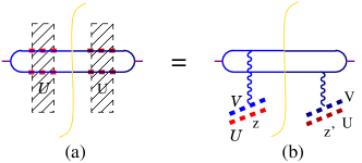
Figure 5: Factorization for the two-gluon exchange.

This formula is easily seen from Fig. (5). Indeed, in the leading order in perturbation theory the l.h.s. of Eq. (44) is represented by the diagram in Fig. 5a where the quark line in the external field ${\cal U}_{i},U_{i}$ is given by

$$\langle\chi(x)\bar{\psi}(y)\rangle~{}=\int\!\!dz\delta(z_{\ast}){\cal U}_{x}(x|{1\over\not\!p}|z)\not\!p_{2}{\cal U}^{\dagger}_{z}U_{z}(z|{1\over\not\!p}|y)U^{\dagger}_{y}$$ (45)

at $x_{\ast},y_{\ast}<0$ (cf. Eq. (11)). On the other hand, the r.h.s. of Eq. (44) is represented by the diagram in Fig. 5b. It is easy to see that the factor $\partial_{\perp}^{2}$ cancels the propagator ${1\over p^{2}}={1\over p_{\perp}^{2}}$ so the diagram in Fig. 5b reduces to 5a.

If we neglect the evolution, the slope of the Wilson lines $U$ can be replaced by $p_{1}$ and the slope of $V$’s by $p_{2}$ (see the discussion in Sec. II.2). The number of particles produced in a collision of weak and strong shock waves (24) is given by the square of the Lipatov vertex (39). Technically it is convenient to introduce a source $\lambda_{i}(x_{\perp})$ for the Lipatov vertex $L_{i}$ ( and $\sigma(x_{\perp})$ for ${\cal L}$) so

$$R(k;U,V,{\cal U},{\cal V})~{}=~{}\int\!d^{2}x_{\perp}d^{2}y_{\perp}~{}e^{i(k,x-y)_{\perp}}~{}{\delta^{2}\over\delta\lambda^{a}_{ix}\delta\sigma^{ia}_{y}}$$

$$\times~{}e^{i\!\int\!d^{2}z_{\perp}[{\cal U}^{a}_{i}{\cal V}^{ai}+\sigma^{ia}(z_{\perp}){\cal L}_{i}^{a}(z_{\perp})-U^{ai}_{z}V^{ai}_{z}-\lambda^{ia}(z_{\perp})L_{i}^{a}(z_{\perp})]}$$

For a weak source $V_{i}\sim\partial_{i}V$ we get $gE_{i}\simeq-(U(g_{ik}+{p_{i}p_{k}\over p_{\perp}^{2}})U^{\dagger})^{ab}V_{k}^{b}$ so $L_{i}(x_{\perp})\simeq 2(x_{\perp}|[{p_{i}\over p_{\perp}^{2}},U]p^{k}U^{\dagger})^{ab}|V^{b}_{k})$ and the above equation can be rewritten as

$$R(k;U,V,{\cal U},{\cal V})~{}=\int\!d^{2}x_{\perp}d^{2}y_{\perp}~{}e^{i(k,x-y)_{\perp}}$$ (46)

$$\times~{}{\delta^{2}\over\delta\lambda^{a}_{i}(x_{\perp})\delta\sigma^{ia}(y_{\perp})}~{}e^{i\!\int\!d^{2}z_{\perp}[\tilde{\cal U}^{a}_{i}(z_{\perp}){\cal V}^{ai}(z_{\perp})-\tilde{U}^{a}_{i}(z_{\perp})V^{ai}(z_{\perp})]}$$

where

$$\tilde{U}~{}=~{}e^{2{\partial_{i}\over\partial_{\perp}^{2}}\lambda}Ue^{-2{\partial^{i}\over\partial_{\perp}^{2}}(U^{\dagger}\lambda U)}$$

$$\tilde{\cal U}~{}=~{}e^{2{\partial_{i}\over\partial_{\perp}^{2}}\sigma}{\cal U}e^{-2{\partial^{i}\over\partial_{\perp}^{2}}({\cal U}^{\dagger}\sigma{\cal U})}$$ (47)

(This expansion is similar to the functional-integral representation of the non-linear evolution as $e^{i\phi_{1}}Ue^{-i\phi_{2}}$ developed in ref. pl ). We need here only the first two terms of the expansion in powers of $\lambda$ and $\sigma$.

Using the simplified factorization formula (44) we get

$$R(k;U,V,{\cal U},{\cal V})$$

$$=~{}{1\over g^{4}}\!\int\!d^{2}x_{\perp}d^{2}y_{\perp}d^{2}z_{\perp}d^{2}z^{\prime}_{\perp}~{}{e^{i(k,x-y)_{\perp}}\over N_{c}^{2}-1}{\delta^{2}\over\delta\lambda^{a}_{ix}\delta\sigma^{ia}_{y}}$$

$$\times~{}{\rm tr}\{\tilde{\cal U}^{\dagger}_{z}\tilde{U}_{z}\tilde{U}^{\dagger}_{z^{\prime}}\tilde{\cal U}_{z^{\prime}}\}\partial_{\perp z}^{2}~{}\partial_{\perp z^{\prime}}^{2}{\rm tr}\{(V^{\dagger}_{z}V_{z^{\prime}}-1)({\cal V}^{\dagger}_{z^{\prime}}{\cal V}_{z}-1)\}$$

$$=~{}{4g^{-2}\over(N_{c}^{2}-1)}\int\!d^{2}x_{\perp}d^{2}y_{\perp}d^{2}z_{\perp}d^{2}z^{\prime}_{\perp}~{}$$

$$\times~{}{\rm tr}\big{\{}\big{[}(y|{p_{i}\over p_{\perp}^{2}}|z)({\cal U}_{z^{\prime}}{\cal U}^{\dagger}_{z}t^{a}-~{}{\cal U}_{z^{\prime}}{\cal U}^{\dagger}_{y}t^{a}{\cal U}_{y}{\cal U}^{\dagger}_{z^{\prime}})$$

$$\hskip 36.98857pt-~{}(y|{p_{i}\over p_{\perp}^{2}}|z^{\prime})(t^{a}{\cal U}_{z^{\prime}}{\cal U}^{\dagger}_{z}-{\cal U}_{z^{\prime}}{\cal U}^{\dagger}_{y}t^{a}{\cal U}_{y}{\cal U}^{\dagger}_{z})\big{]}$$

$$\times~{}\big{[}(x|{p^{i}\over p_{\perp}^{2}}|z)(t^{a}U_{z}U^{\dagger}_{z^{\prime}}-U_{z}U^{\dagger}_{x}t^{a}U_{x}U^{\dagger}_{z^{\prime}})$$

$$\hskip 36.98857pt-~{}(x|{p^{i}\over p_{\perp}^{2}}|z^{\prime})(U_{z}U^{\dagger}_{z^{\prime}}t^{a}-U_{z}U^{\dagger}_{x}t^{a}U_{x}U^{\dagger}_{z^{\prime}})\big{]}\big{\}}$$

$$\times~{}e^{i(k,x-y)_{\perp}}\partial_{\perp z}^{2}~{}\partial_{\perp z^{\prime}}^{2}{\rm tr}\{(V^{\dagger}_{z}V_{z^{\prime}}-1)({\cal V}^{\dagger}_{z^{\prime}}{\cal V}_{z}-1)\}$$ (48)

Without evolution, ${\cal U}\equiv U$ and ${\cal V}\equiv V$ so the square of the Lipatov vertex (48) reduces to

$$R(k_{\perp};U,V)~{}$$ (49)

$$=~{}{2g^{-2}\over N_{c}^{2}-1}\!\int\!d^{2}z_{\perp}d^{2}z^{\prime}_{\perp}~{}{\rm tr}\{\partial_{\perp}^{2}V_{z}~{}\partial_{\perp}^{2}V^{\dagger}_{z^{\prime}}+z\leftrightarrow z^{\prime}\}$$

$$\times~{}{\rm Tr}\big{\{}\big{(}(k_{\perp}|[{p_{i}\over p_{\perp}^{2}},U]|z_{\perp})-\big{(}(k_{\perp}|[{p_{i}\over p_{\perp}^{2}},U]|z^{\prime}_{\perp})\big{)}$$

$$\times~{}\big{(}(z_{\perp}|[{p^{i}\over p_{\perp}^{2}},U^{\dagger}]|k_{\perp})-(z^{\prime}_{\perp}|[{p^{i}\over p_{\perp}^{2}},U^{\dagger}]|k_{\perp})\big{)}\big{\}}$$

It is easy to see that in the momentum representation we get

$$R(k_{\perp};U,V)~{}=~{}{2g^{-2}\over N_{c}^{2}-1}\!\int\!d^{2}k^{\perp}_{1}d^{2}k^{\perp}_{2}~{}K^{\rm emi}_{\rm BFKL}(k_{1},k_{2};k)$$

$$\times~{}{\rm tr}\{V(k^{\perp}_{1})V^{\dagger}(-k^{\perp}_{2})\}{\rm tr}\{U(k_{\perp}-k^{\perp}_{1})U^{\dagger}(k^{\perp}_{2}-k^{\perp})\}$$ (50)

where

$$K^{\rm emi}_{\rm BFKL}(k_{1},k_{2};k)=-2\Big{(}{k^{i}\over k_{\perp}^{2}}k_{1\perp}^{2}-k_{1}^{i}\Big{)}\Big{(}{k_{i}\over k_{\perp}^{2}}k_{2\perp}^{2}-k_{2i}\Big{)}$$

$$=~{}{k_{1\perp}^{2}(k-k_{2})_{\perp}^{2}\over k_{\perp}^{2}}+{k_{2\perp}^{2}(k-k_{1})_{\perp}^{2}\over k_{\perp}^{2}}-(k_{1}-k_{2})_{\perp}^{2}$$ (51)

is the gluon-emission part of the BFKL kernel bfkl .

Substituting the result of the integration over central-rapidity gluons (49) into the factorization formula (5) we obtain the standard $k_{T}$-factorization formula

$$n_{g}(k_{\perp};\eta)) = {2g^{-2}\over N_{c}^{2}-1}\!\int\!\!d^{2}k_{1}d^{2}k_{2}K^{\rm emi}_{\rm BFKL}(k_{1},k_{2};k_{\perp})$$ (52)

$$\times \langle A|{\rm Tr}\{V(k_{1})V^{\dagger}(-k_{2})|A\rangle$$

$$\times \langle B|{\rm Tr}\{U(k_{\perp}-k_{1})U^{\dagger}(k_{\perp}-k_{2})|B\rangle$$

where the rapidity dependence comes from the slope of the Wilson lines in the r.h.s. This formula was obtained in the approximation when we neglect the evolution of the shock waves, but it can be proved without this assumption mabraun1 ; kovtuchin ; xapkovtuchin ; saclay . It should be emphasized that Eq. (52) is valid only in the first order in the $[U,V]$ expansion (that is, for the $pA$ scattering). As we shall see below, it is not valid beyond the first order.

VI Effective action

In this section we get the first-order effective action for the double functional integral (1) and check that the Lipatov vertex (43) serves as a “splitting function” for the non-linear evolution equation npb96 ; yura

$${\partial\over\partial\eta}{\rm Tr}\{U_{x}U^{\dagger}_{y}\}~{}=~{}-{\alpha_{s}\over 4\pi}\!\int\!d^{2}z_{\perp}{(x-y)_{\perp}^{2}\over(x-z)_{\perp}^{2}(y-z)_{\perp}^{2}}$$

$$\times({\rm Tr}\{U_{x}U^{\dagger}_{z}\}{\rm Tr}\{U_{z}U^{\dagger}_{y}\}-N_{c}{\rm Tr}\{U_{x}U^{\dagger}_{y}\})$$ (53)

The effective action is defined by the functional integral (24) without $A_{\mu}(p)A^{\mu}(-p)$ insertion:

$$e^{iS_{\rm eff}(U,V,{\cal U},{\cal V})}~{}=~{}\int\!\!D{\cal A}DA~{}\exp\Big{\{}-iS({\cal A})$$ (54)

$$+~{}i\!\int\!d^{2}z\Big{(}{\cal V}^{ai}_{z}[\infty,{\cal F}_{\ast i},\infty]^{a}_{z}+~{}(\infty,{\cal F}_{\ast i},\infty)^{a}_{z}{\cal U}^{ai}_{z}\Big{)}$$

$$+~{}iS(A)-i\!\!\int\!\!d^{2}z\Big{(}V^{ai}_{z}[\infty,F_{\ast i},\infty]^{a}_{z}+(\infty,F_{\ast i},\infty)^{a}_{z}U^{ai}_{z}\Big{)}\Big{\}}$$

Performing the shift $A\rightarrow A+\bar{A}_{i}^{(0)}$, ${\cal A}\rightarrow{\cal A}+\bar{\cal A}_{i}^{(0)}$ we get (cf. Eq. (26)

$$e^{iS_{\rm eff}(U,V,{\cal U},{\cal V})}~{}=~{}\int\!D{\cal A}DA\exp\Big{\{}i\!\int\!d^{4}z\Big{(}({1\over 2}{\cal A}^{\mu}\bar{\cal D}_{\mu\nu}{\cal A}^{\nu}$$

$$-~{}{1\over 2}A^{\mu}\bar{D}_{\mu\nu}A^{\nu}-{\cal T}^{\mu}{\cal A}_{\mu}+T^{\mu}A_{\mu}\Big{)}\Big{\}}$$ (55)

The effective action in the first nontrivial order is given by the integration of linear terms with the appropriate Green functions

$$iS_{\rm eff}(U,V,{\cal U},{\cal V})~{}=~{}$$

$${1\over 2}\!\int\!d^{4}zd^{4}z^{\prime}\Big{\{}-T^{a}_{\mu}(z)\langle A^{\mu a}(z)A^{\nu b}(z^{\prime})\rangle T^{b}_{\nu}(z^{\prime})$$

$$\hskip 56.9055pt+~{}2T^{a}_{\mu}(z)\langle A^{\mu a}(z){\cal A}^{\nu b}(z^{\prime})\rangle{\cal T}^{b}_{\nu}(z^{\prime})$$

$$\hskip 56.9055pt-~{}{\cal T}^{a}_{\mu}(z)\langle{\cal A}^{\mu a}(z){\cal A}^{\nu b}(z^{\prime})\rangle{\cal T}^{b}_{\nu}(z^{\prime})\Big{\}}$$

The first term here can be taken from prd99 ; mobzor :

$$iS^{(1)}_{\rm eff}(U,V)~{}=$$ (56)

$$\alpha_{s}\Delta\eta\int\!d^{2}z\Big{(}E^{a}_{i}E^{ai}+[U_{i},V^{i}+2E^{i}]{1\over\partial^{2}_{\perp}}[V_{i},U^{i}+2E^{i}]\Big{)}$$

where $\Delta\eta=\eta_{1}-\eta_{2}$ is the difference of rapisdities of the slopes of $U$ and $V$ Wilson lines. The third term $S^{(1)}_{\rm eff}({\cal U},{\cal V})$ in Eq. (VI) is obtained from Eq. (56) by the usual replacements $U\leftrightarrow\cal{U}$, $V\leftrightarrow\cal{V}$

Let us calculate the second term beginning with the contribution $\sim[U_{i},V^{i}]...[{\cal U}^{i},{\cal V}^{i}]$. The Green function in the $x_{\ast},x_{\bullet}>0$ sector is simply the perturbative propagator (2) so one obtains

$$-g^{2}\!\!\int\!{d\alpha d\beta\over 2\pi^{2}\alpha\beta}(0,[{\cal U}^{i},{\cal V}_{i}]^{a}|2\pi\delta(\alpha\beta s-p^{2}_{\perp})\theta(\alpha)|0,[U^{i},V_{i}]^{a})$$

$$=~{}-g^{2}([U^{i},V_{i}]^{a}|{1\over p_{\perp}^{2}}[U^{i},V_{i}]^{a})\int_{0}^{\infty}\!{d\alpha\over\pi\alpha}$$ (57)

The integral (57) is formally divegrent at both small and large $\alpha$. This divergence occurs because we’ve put the slopes of Wilson lines $e_{1}$ and $e_{2}$ (see Eq. (21)) to be $p_{1}$ and $p_{2}$. If we keep the slopes off the light cone, we get (see ref. mobzor ):

$$-g^{2}\!\int\!{d\alpha d\beta\over 2\pi^{2}}{1\over(\alpha+e^{-\eta_{1}}\beta)(\beta+e^{\eta_{2}}\alpha)}$$

$$\times~{}(0,[{\cal U}^{i},{\cal V}_{i}]^{a}|2\pi\delta(\alpha\beta s-p^{2}_{\perp})\theta(\alpha)|0,[U^{i},V_{i}]^{a})~{}$$

$$=~{}-2\alpha_{s}\Delta\eta([{\cal U}^{i},{\cal V}_{i}]^{a}|{1\over p_{\perp}^{2}}[U^{i},V_{i}]^{a})$$ (58)

The contributions of $[U_{i},V_{k}]-i\leftrightarrow k$ terms can be calculated in a similar manner by integration of these terms with appropriate Green functions in Eq. (56). After some algebra, one obtains

$$-2\alpha_{s}\Delta\eta\Big{\{}\!\int\!d^{2}z_{\perp}{\cal E}^{i}E_{i}(z_{\perp})+({\cal U}^{i}-{\cal V}_{i},{\cal E}^{i}]^{a}|{1\over p_{\perp}^{2}}|[U^{i},V_{i}]^{a})$$

$$+~{}([{\cal U}^{i},{\cal V}_{i}]^{a}|{1\over p_{\perp}^{2}}|[U^{i}-V_{i},E^{i}]^{a})\Big{\}}$$ (59)

The sum of Eqs. (58) and (59) give the second term in the effective action

$$iS^{(2)}_{\rm eff}(U,V,{\cal U},{\cal V})~{}=$$

$$-\alpha_{s}\Delta\eta\int\!d^{2}z\Big{(}2{\cal E}^{ai}E^{a}_{i}+[{\cal U}_{i},{\cal V}^{i}+2{\cal E}^{i}]{1\over\partial^{2}_{\perp}}[V_{i},U^{i}+2E^{i}]$$

$$+~{}[{\cal V}_{i},{\cal U}^{i}+{\cal E}^{i}]{1\over\partial^{2}_{\perp}}[U_{i},V^{i}+E^{i}]\Big{)}$$ (60)

It is easy to see that the total effective action $S_{\rm eff}(U,V,{\cal U},{\cal V})=S^{(1)}_{\rm eff}(U,V)+S^{(2)}_{\rm eff}(U,V,{\cal U},{\cal V})+S^{(3)}_{\rm eff}({\cal U},{\cal V})$ can be represented as

$$iS_{\rm eff}(U,V,{\cal U},{\cal V})~{}=~{}-i{\cal U}_{i}{\cal V}^{i}+iU_{i}V^{i}$$ (61)

$$+{\alpha_{s}\over 4}\Delta\eta\int\!d^{2}z\Big{(}L^{a}_{i}L^{ai}-2{\cal L}^{ai}L^{a}_{i}+{\cal L}^{ai}{\cal L}^{a}_{i}\Big{)}$$

where $L_{i}$ and ${\cal L}_{i}$ are given by Eq. (43). Note that the effective action is a square of Lipatov vertex (39): $R_{\mu}R^{\mu}=L_{i}L^{i}$, ${\cal R}_{\mu}R^{\mu}={\cal L}_{i}L^{i}$, ${\cal R}_{\mu}{\cal R}^{\mu}={\cal L}_{i}{\cal L}^{i}$.

For the future applications we will rewrite the effective action (61) as a Gaussian integration over the auxiliary field $\lambda$ coupled to Lipatov vertex (43):

$$e^{iS_{\rm eff}(U,V,{\cal U},{\cal V})}~{}=~{}e^{i\int d^{2}z_{\perp}(-{\cal U}_{i}{\cal V}^{i}+U_{i}V^{i})}$$ (62)

$$\times~{}\int D\lambda\exp\Big{\{}\int\!d^{2}z_{\perp}\Big{(}-{\lambda^{a}_{i}\lambda^{ai}\over\alpha_{s}\Delta\eta}+(L^{a}_{i}-{\cal L}^{ai})\lambda^{a}_{i}\Big{)}\Big{\}}$$

A single field $\lambda_{i}$ for both $L_{i}$ and ${\cal L}_{i}$ reflects the fact that gauge fields $A_{\mu}$ and ${\cal A}_{\mu}$ coincide at $t=\infty$.

Let us prove now that the effective action (62) agrees with the non-linear evolution equation. To find the evolution of the dipole $U_{x}U^{\dagger}_{y}$, we need to consider the effective action for the weak source $V$. As we mentioned above, at small $V_{i}\sim\partial_{i}V$ one has $gE_{i}\simeq-(U(g_{ik}+{p_{i}p_{k}\over p_{\perp}^{2}})U^{\dagger})^{ab}V_{k}^{b}$ so $L_{i}(x_{\perp})\simeq 2(x_{\perp}|[{p_{i}\over p_{\perp}^{2}},U]p^{k}U^{\dagger})^{ab}|V^{b}_{k})$ and Eq. (62) can be rewritten as

$$\int\!D{\cal A}DA\exp\Big{\{}-iS({\cal A})+iS(A)$$ (63)

$$-~{}i\!\int\!d^{2}z_{\perp}{\cal V}^{ai}_{z}[\infty,{\cal F}_{\ast i},\infty]^{a}_{z}-i\!\int\!d^{2}z_{\perp}(\infty,{\cal F}_{\ast i},\infty)^{a}_{z}{\cal U}^{ai}_{z}$$

$$+~{}i\!\int\!d^{2}z_{\perp}V^{ai}_{z}[\infty,F_{\ast i},\infty]^{a}_{z}+i\!\int\!d^{2}z_{\perp}(\infty,F_{\ast i},\infty)^{a}_{z}U^{ai}_{z}\Big{\}}$$

$$=\int D\lambda\exp\Big{\{}\int\!d^{2}z_{\perp}\Big{(}-{\lambda^{a}_{i}\lambda^{ai}\over\alpha_{s}\Delta\eta}-i{\cal V}_{i}\tilde{\cal U}^{i}+iV_{i}\tilde{U}^{i}\Big{)}\Big{\}}$$

where

$$\tilde{U}~{}=~{}e^{2{\partial_{i}\over\partial_{\perp}^{2}}\lambda}Ue^{-2{\partial^{i}\over\partial_{\perp}^{2}}(U^{\dagger}\lambda U)}$$

$$\tilde{\cal U}~{}=~{}e^{2{\partial_{i}\over\partial_{\perp}^{2}}\lambda}{\cal U}e^{-2{\partial^{i}\over\partial_{\perp}^{2}}({\cal U}^{\dagger}\lambda{\cal U})}$$ (64)

Again,we need here only the terms up to the second order in $\lambda$.

To find the evolution of the dipole $U_{x}U^{\dagger}_{y}$ we should expand Eq. (63) in powers of $V_{i}({\cal V}_{i})$ and use the formula $(U_{x}U^{\dagger}_{y})^{\eta_{2}}=Pe^{ig\!\int_{x}^{y}\!dz_{i}[\infty,F_{\ast i},\infty]_{z}}$. We get

$$(U_{x}U^{\dagger}_{y}{\cal U}_{y}{\cal U}^{\dagger}_{x})^{\eta_{1}}$$

$$~{}=\int D\lambda~{}e^{-{1\over\alpha_{s}\Delta\eta}\int\!d^{2}z_{\perp}\lambda^{a}_{i}\lambda^{ai}}~{}\tilde{U}_{x}\tilde{U}^{\dagger}_{y}\tilde{\cal U}_{y}\tilde{\cal U}^{\dagger}_{y}$$ (65)

Performing the Gaussian integration over $\lambda$ one obtains after some algebra

$${\rm tr}(U_{x}U^{\dagger}_{y}{\cal U}_{y}{\cal U}^{\dagger}_{x})^{\eta_{1}}$$ (66)

$$=~{}{\rm tr}\{U_{x}U^{\dagger}_{y}{\cal U}_{y}{\cal U}^{\dagger}_{x}\}^{\eta_{2}}+{\alpha_{s}\Delta\eta\over 4\pi^{2}}\!\int\!d^{2}z_{\perp}{(x-y)_{\perp}^{2}\over(x-z)_{\perp}^{2}(z-y)_{\perp}^{2}}$$

$$\times~{}({\rm tr}\{{\cal U}^{\dagger}_{x}U_{x}U^{\dagger}_{z}{\cal U}_{z}\}{\rm tr}\{{\cal U}^{\dagger}_{z}U_{z}U^{\dagger}_{y}{\cal U}_{y}\}-N_{c}{\rm tr}\{{\cal U}^{\dagger}_{x}U_{x}U^{\dagger}_{y}{\cal U}_{y}\})^{\eta_{2}}$$

which is the non-linear evolution equation for the double functional integral for the cross section difope ; mobzor .

VII Classical fields and Lipatov vertex in the second order

If we neglect the evolution, the classical sources $U_{i}$ and ${\cal U}_{i}$ coincide (and similarly $V_{i}={\cal V}_{i}$) so the corresponding fields in the right and left sectors coincide and are determined by the integrals of the retarded Green functions with the ${\cal T}=T$ sources.

VII.1 First-order gluon field in the $x_{\parallel}^{\mu}A_{\mu}=0$ gauge

Figure 6: Retarded classical field in the first order

In the first order in $[U,V]$, the classical fields (38) (in the background gauge) reduce to

$${\bar{A}}_{i}^{(1)} = W_{i}(x_{\perp})\theta(-x_{\ast})\theta(-x_{\bullet})+~{}U_{i}(x_{\perp})\theta(-x_{\ast})\theta(x_{\bullet})$$

$$+ V_{i}(x_{\perp})\theta(x_{\ast})\theta(-x_{\bullet})+2g(x|{1\over p^{2}+i\epsilon p_{0}}|0,E_{i})$$

$$\bar{A}_{\bullet}^{(1)} = g(x|{(\alpha+i\epsilon)^{-1}\over p^{2}+i\epsilon p_{0}}|0,[U_{i},V^{i}])$$

$$\hskip 71.13188pt+~{}g(x|{(\alpha-i\epsilon)^{-1}\over p^{2}+i\epsilon p_{0}}|0,[U_{i},E^{i}])$$

$$\bar{A}_{\ast}^{(1)} = -g(x|{(\beta+i\epsilon)^{-1}\over p^{2}+i\epsilon p_{0}}|0,[U_{i},V^{i}])$$

$$\hskip 71.13188pt+~{}g(x|{(\beta-i\epsilon)^{-1}\over p^{2}+i\epsilon p_{0}}|0,[V_{i},E^{i}])$$

$$\bar{A}_{i}^{(1)} = 2g(x|{1\over p^{2}+i\epsilon p_{0}}|0,E_{i})$$ (67)

We see that the fields outside the forward cone are piece-wise pure gauge:

$${\bar{A}}_{i}^{(1)}~{}=~{}W_{i}(x_{\perp})\theta(-x_{\ast})\theta(-x_{\bullet})+~{}U_{i}(x_{\perp})\theta(-x_{\ast})\theta(x_{\bullet})$$

$$\hskip 56.9055pt+~{}V_{i}(x_{\perp})\theta(x_{\ast})\theta(-x_{\bullet})$$

$$\bar{A}_{\bullet}^{(1)}~{}=~{}-ig\delta(x_{\ast})\theta(-x_{\bullet})(x_{\perp}|{1\over p_{\perp}^{2}}|[U_{i},E^{i}]),$$

$$\bar{A}_{\ast}^{(1)}~{}=~{}-ig\delta(x_{\bullet})\theta(-x_{\ast})(x_{\perp}|{1\over p_{\perp}^{2}}|[V_{i},E^{i}])$$ (68)

while the field in the forward sector $x_{\ast},x_{\bullet}>0$ is determined by the Lipatov vertex (39).

$$\bar{A}_{\mu}^{(1)}~{}=~{}(x|{1\over p^{2}+i\epsilon p_{0}}|R_{\mu})$$ (69)

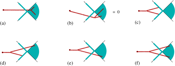
Figure 7: Classical field in the second order in $[U,V]$

Summarising, the classical field (67) can be represented as

$${\bar{A}}_{\mu}^{(1)} = \tilde{A}_{\perp\mu}+(x|{1\over p^{2}+i\epsilon p_{0}}|R^{(1)}_{\mu})$$ (70)

where

$$\tilde{A}_{i} = \theta(-x_{\ast})\theta(x_{\bullet})U_{i}(x_{\perp})$$

$$+ \theta(x_{\ast})\theta(-x_{\bullet})V_{i}(x_{\perp})+\theta(-x_{\ast})\theta(-x_{\bullet})W_{i}(x_{\perp})$$

is a trivial part corresponding to a piece-wise pure-gauge field and

$$R^{(1)}_{\mu}=2gE^{\perp}_{\mu}+g{2p_{2\mu}\over s}\Big{(}{1\over\alpha+i\epsilon}[U_{i},V^{i}]+{2\over\alpha-i\epsilon}[U_{i},E^{i}]\Big{)}$$

$$+~{}g{2p_{1\mu}\over s}\Big{(}{1\over\beta+i\epsilon}[V_{i},U^{i}]+{2\over\beta+i\epsilon}[V_{i},E^{i}]\Big{)}$$ (72)

describes the non-trivial part related to the gluon emission.

The axial-gauge Lipatov vertex is given by first line in Eq. (43):

$$L_{i}(U,V)~{}=~{}2gE_{i}-2ig{\partial_{i}\over\partial_{\perp}^{2}}[U_{j}+2E_{j},V^{j}]$$ (73)

Following ref. nncoll , it is instructive to represent the fields (67) in the gauge $x^{\parallel}_{\mu}A^{\mu}=x_{\ast}A_{\bullet}+x_{\bullet}A_{\ast}=0$. In this gauge one obtains at $x_{\ast},x_{\bullet}>0$

$$A^{\parallel}_{\mu}(x_{\parallel},x_{\perp})~{}=~{}-\int_{1}^{\infty}\!udu~{}x_{\parallel}^{\rho}F_{\rho\mu}(ux_{\parallel},x_{\perp}),$$

$$A^{\perp}_{\mu}(x_{\parallel},x_{\perp})~{}=~{}-\int_{1}^{\infty}\!du~{}x_{\parallel}^{\rho}F_{\rho\mu}(ux_{\parallel},x_{\perp})$$ (74)

where $x_{\parallel}\equiv{2\over s}x_{\ast}p_{1}+{2\over s}x_{\bullet}p_{2}$ (so that $x=x_{\parallel}+x_{\perp}$). The limit of integration $\infty$ in the above expressions was chosen to satisfy our boundary condition (no pure gauge fields at $t=\infty$ .

The fields ouside the forward cone (68) trivially satisfy the $x^{\parallel}_{\mu}A^{\mu}=0$ gauge condition. The fields in the forward cone $x_{\ast},x_{\bullet}>0$ are obtained by integrating $F_{\mu\nu}$’s corresponding to the fileds in the bF gauge (67). From the Eq. (74) we get:

$$\bar{A}_{\ast}(x)~{}=~{}i{gs\over 8\pi x_{\bullet}}\!\int\!d^{2}z_{\perp}\theta(-x_{\parallel}^{2}+(x-z)_{\perp}^{2})$$

$$\hskip 56.9055pt\times~{}(2[U_{i},V^{i}]+[U_{i}-V_{i},E^{i}])$$ (75)

$$\bar{A}_{\bullet}^{\rm MV}(x)~{}=~{}-i{gs\over 8\pi x_{\ast}}\!\int\!d^{2}z_{\perp}\theta(-x_{\parallel}^{2}+(x-z)_{\perp}^{2})$$

$$\hskip 56.9055pt\times~{}(2[U_{i},V^{i}]+[U_{i}-V_{i},E^{i}])$$

$$\bar{A}_{i}(x)~{}=~{}-{g\over\pi}\!\int\!d^{2}z_{\perp}\delta(x_{\parallel}^{2}-(x-z)_{\perp}^{2})E_{i}$$

$$+~{}g\!\int\!d^{2}z_{\perp}\theta(-x_{\parallel}^{2}+(x-z)_{\perp}^{2})(x_{\perp}|{p_{i}\over p_{\perp}^{2}}|z_{\perp})[U_{j}+V_{j},E^{j}]$$

Similarly to ref. nncoll , the fields $x_{\ast}A^{(1)}_{\bullet}$, $x_{\bullet}A^{(1)}_{\ast}$ and $A^{(1)}_{i}$ are boost invariant. However, as we mentioned in the footnote, the fields (75) differ from those in ref. nncoll due to a different boundary condition.

VII.2 Gluon field and Lipatov vertex in the second order in $[U,V]$

In the next order the classical field $\bar{A}^{(2)}$ is given by diagrams in Fig. 7 calculated in the Appendix C. The result of the calculation is given by the sum of the piece-wise pure gauge field and the field of the gluon emission described by the second-order Lipatov vertex represented by two terms coming from the diagrams in Fig. 6 and Fig. 7

$${\bar{A}}_{i} = \theta(-x_{\ast})\theta(-x_{\bullet})W_{i}(x_{\perp})$$

$$+ \theta(-x_{\ast})\theta(x_{\bullet})U_{i}(x_{\perp})+\theta(x_{\ast})\theta(-x_{\bullet})V_{i}(x_{\perp})$$

$$+ (x|{1\over p^{2}+i\epsilon p_{0}}|R^{(1)}_{\mu}+R^{(2)}_{\mu})~{}+~{}O([U,V]^{3})$$

The first part of the Lipatov vertex coming from the diagrams in Fig. 6 and Fig. 7a has the form

$$R^{\rm(1)}_{\mu}(k)~{}=~{}R^{\rm(1)}_{\perp\mu}(k_{\perp})+{2p_{1\mu}\over s}\Big{(}{R_{1+}^{\rm(1)}(k_{\perp})\over\beta+i\epsilon}+{R_{1-}^{\rm(1)}(k_{\perp})\over\beta-i\epsilon}\Big{)}$$

$$+~{}{2p_{2\mu}\over s}\Big{(}{R_{2+}^{\rm(1)}(k_{\perp})\over\alpha+i\epsilon}+{R_{2-}^{\rm(1)}(k_{\perp})\over\alpha-i\epsilon}\Big{)}$$ (77)

where the notations are

$$(R^{\rm(1)}_{\perp\mu})^{a}~{}=~{}2gE_{\perp\mu}+4ig((\partial^{\perp}_{\mu}U){1\over p_{\perp}^{2}}U^{\dagger})^{ab}[V_{i},E^{i}]^{b}$$

$$\hskip 71.13188pt+~{}4ig((\partial^{\perp}_{\mu}V){1\over p_{\perp}^{2}}V^{\dagger})^{ab}[U_{i},E^{i}]^{b}$$

$$(R_{1+}^{\rm(1)})^{a}~{}=~{}-g[U_{i},V^{i}]^{a}-2g((\partial_{\perp}^{2}V){1\over p_{\perp}^{2}}V^{\dagger})^{ab}[U_{i},E^{i}]^{b}$$

$$(R_{1-}^{\rm(1)})^{a}~{}=~{}2gp_{\perp}^{2}(U{1\over p_{\perp}^{2}}U^{\dagger})^{ab}[V_{i},E^{i}]^{b}$$

$$(R_{2+}^{\rm(1)})^{a}~{}=~{}g[U_{i},V^{i}]^{a}-2g((\partial_{\perp}^{2}U){1\over p_{\perp}^{2}}U^{\dagger})^{ab}[V_{i},E^{i}]^{b}$$

$$(R_{2-}^{\rm(1)})^{a}~{}=~{}2gp_{\perp}^{2}(V{1\over p_{\perp}^{2}}V^{\dagger})^{ab}[U_{i},E^{i}]^{b}$$ (78)

The second-order term coming from the diagrams in Fig. 7c-f is given by

$$R^{\rm(2)~{}a}_{\mu}(k)~{}=~{}f^{abc}\!\int\!{d^{2}k^{\prime}_{\perp}\over 32\pi^{2}}\Bigg{\{}-{1\over\sqrt{\cal G}}[K_{\mu}g_{\mu\eta}-~{}2(k_{\xi}g_{\mu\eta}$$

$$-~{}(k_{\eta}g_{\mu\xi})]\tilde{R}^{b\xi}(k_{\perp})\tilde{R}^{c}_{\xi}(k_{\perp}-k^{\prime}_{\perp})+8i\Big{(}{p_{2}\over\alpha s}-{p_{1}\over\beta s}\Big{)}_{\mu}$$

$$\times~{}{(k^{\prime},k-k^{\prime})_{\perp}+{k^{2}\over 2}-i\sqrt{\cal G}\over{k^{\prime}}_{\perp}^{2}(k-k^{\prime})_{\perp}^{2}}R_{1}^{b}(k^{\prime}_{\perp})R_{2}^{c}(k_{\perp}-k^{\prime}_{\perp})$$

$$+~{}32i{k^{\xi}\delta_{\mu}^{\eta}-k^{\eta}\delta_{\mu}^{\xi}\over{k^{\prime}}_{\perp}^{2}}\Big{(}{p_{1\xi}\over\beta s}R_{1-}^{b}(k^{\prime}_{\perp})+{p_{2\xi}\over\alpha s}R_{2-}^{b}(k^{\prime}_{\perp})\Big{)}$$

$$\times~{}gE_{\eta}^{\perp c}(k_{\perp}-k^{\prime}_{\perp})\Bigg{\}}$$ (79)

$$+~{}g^{2}\Big{(}{4p_{1}\over\beta s}-~{}{4p_{2}\over\alpha s}\Big{)}_{\mu}(k_{\perp}|[U_{i},V^{i}]^{ab}{1\over p_{\perp}^{2}}|[U_{j}+V_{j},E^{j}]^{b})$$

where we use the notations

$$K\equiv(k-2k^{\prime})_{\perp}+{k^{\parallel}\over\alpha\beta s}(k,k-2k^{\prime})_{\perp}$$ (80)

$${\cal G}~{}=~{}{k^{\prime}}_{\perp}^{2}(k-k^{\prime})_{\perp}^{2}-\Big{(}{k^{2}+i\epsilon k_{0}\over 2}+(k^{\prime},k-k^{\prime})_{\perp})\Big{)}^{2}$$ (81)

$$\tilde{R}_{\xi}(k^{\prime}_{\perp})=2E_{\perp\xi}(k^{\prime}_{\perp})$$ (82)

$$+~{}{(k,k^{\prime})_{\perp}+{k^{2}\over 2}-i\sqrt{\cal G}\over{k^{\prime}}_{\perp}^{2}}\Big{(}{2p_{1}\over\beta s}R_{1}(k^{\prime}_{\perp})+{2p_{2}\over\alpha s}R_{2}(k^{\prime}_{\perp})\Big{)}_{\xi}$$

and $R_{1}^{\rm(1)}\equiv R_{1+}^{\rm(1)}+R_{1-}^{\rm(1)}$, $R_{2}^{\rm(1)}\equiv R_{2+}^{\rm(1)}+R_{2-}^{\rm(1)}$.
With $[U,V]^{2}$ accuracy $R_{1}^{\rm(1)}$ and $R_{2}^{\rm(1)}$ in Eq. (79) can be simplified to

$$(R_{1}^{\rm(1)})^{a}~{}=~{}-g[U_{i},V^{i}]^{a}+2gp_{\perp}^{2}(U{1\over p_{\perp}^{2}}U^{\dagger})^{ab}[V_{i},E^{i}]^{b}$$

$$(R_{2}^{\rm(1)})^{a}~{}=~{}g[U_{i},V^{i}]^{a}+2gp_{\perp}^{2}(V{1\over p_{\perp}^{2}}V^{\dagger})^{ab}[U_{i},E^{i}]^{b}$$ (83)

The second-order Lipatov vertex is the the sum of Eqs. (77) and (79) at the mass shell $k^{2}=0$. At the first sight, it looks like the expression (79) is divergent at $k^{\prime}_{\perp}\parallel k_{\perp}$ since ${\cal G}=k_{\perp}^{2}{k^{\prime}}^{2}(1-\cos^{2}\theta)$. This collinear divergence is however purely longitudinal and therefore can be eliminated by proper gauge transformation. To see that, let us write the Lipatov vertex in the axial light-like gauge $p_{2}^{\mu}A_{\mu}=0$ (41). As we mentioned above, only the first transverse term in r.h.s. of Eq. (41) is essential since $p_{2}$ term does not contribute to the square of the Lipatov vertex. For this transverse part we obtain

$$L_{i}(k_{\perp})~{}=~{}L^{\rm(1)}_{i}(k_{\perp})+L^{\rm(2)}_{i}(k_{\perp})~{}$$ (84)

$$L^{\rm(1)}_{i}(k_{\perp})~{}=~{}R^{\rm(1)}_{i}(k_{\perp})+{2k_{i}\over k_{\perp}^{2}}(R_{1+}^{\rm(1)}(k_{\perp})+R_{1-}^{\rm(1)}(k_{\perp}))$$

$$L^{\rm(2)~{}a}_{i}(k_{\perp})~{}=~{}f^{abc}\!\int\!{d^{2}k^{\prime}_{\perp}\over 4\pi^{2}}{1\over\sqrt{k_{\perp}^{2}{k^{\prime}}_{\perp}^{2}-(k,k^{\prime})_{\perp}^{2}}}$$ (85)

$$\times~{}\Bigg{\{}{1\over 8}\Big{(}g_{ij}+{k_{i}k_{j}\over k_{\perp}^{2}}\Big{)}(2k^{\prime}-k)^{j}L^{(1)b}_{l}(k^{\prime}_{\perp})L^{(1)cl}(k_{\perp}-k^{\prime}_{\perp})$$

$$+~{}{1\over 2}(k_{j}-{(k,k^{\prime})_{\perp}\over{k^{\prime}}_{\perp}^{2}}k^{\prime}_{j})L^{(1)bj}(k^{\prime}_{\perp})L^{(1)c}_{i}(k_{\perp}-k^{\prime}_{\perp})\Bigg{\}}$$

$$+~{}if^{abc}\!\int\!{d^{2}k^{\prime}_{\perp}\over 4\pi^{2}{k^{\prime}}_{\perp}^{2}}\Bigg{[}2[U_{j}+V_{j},E^{j}]^{b}(k^{\prime}_{\perp})E_{i}^{c}(k_{\perp}-k^{\prime}_{\perp})$$

$$+~{}2{k_{i}k^{j}\over k_{\perp}^{2}}[U_{l}-2E_{l},V^{l}]^{b}(k^{\prime}_{\perp})E_{j}^{c}(k_{\perp}-k^{\prime}_{\perp})$$

$$-~{}\Big{(}{k^{\prime}_{i}\over(k-k^{\prime})_{\perp}^{2}}+{k_{i}\over k_{\perp}^{2}}\Big{)}(R_{1}^{\rm(1)})^{b}(k^{\prime}_{\perp})(R_{2}^{\rm(1)})^{c}(k_{\perp}-k^{\prime}_{\perp})\Bigg{]}$$

$$-~{}4{k_{i}\over k_{\perp}^{2}}(k_{\perp}|[U_{i},V^{i}]^{ab}{1\over p_{\perp}^{2}}|[U_{j}+V_{j},E^{j}]^{b})$$

Note that since the square bracket in the r.h.s. of the above equation vanishes at $k^{\prime}_{\perp}\parallel k_{\perp}$, the collinear divergrnce is absent. The second-order Lipatov vertex (84) is the main technical result of this paper.

VIII Conclusions and outlook

Let us summarize the progress towards the solution of the main problem - the particles/fields produced in the collision of two shock waves. The Yang-Mills equations with sources $U$ and $V$ describe the two shock waves corresponding to the colliding hadrons. The expansion of the classical fields in commutators $[U,V]$ has the advantage of being “symmetric” in contrast to the usual expansion in powers of the strength of one of the sources. We have calculated the second nontrivial term of the expansion. This term is relevant for the description of $dA$ scattering, similar to the first term $\sim[U,V]$ describing the $pA$ collisions.

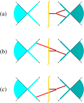
Figure 8: Classical field for ${\cal U}\neq U$, ${\cal V}\neq V$,

Note that while the first-order field given by Eq. (70) (or Eq. (75)) is real, the second-order field has an imaginary part given by the second term in braces in Eq. (79). The real part of the second-order term is given by Eq. (77) plus the first expression in braces in Eq. (79) represented by the product of first-order Lipatov vertices. I think that this univeral structure will survive to the higher orders of the commutator expansion. Unfortunately, the explicit form of the imaginary part of the field (second term in the r.h.s of the Eq. (85)) does not suggest any idea how this expression may look in higher orders in $[U,V]$ expansion. Technically, the relative simplicity of the real part is a consequence of its relation to the leading log approximation (LLA). If we consider the general case ${\cal U}\neq U$, ${\cal V}\neq V$, the second-order classical field would contain $\Delta\eta$ just like the effective action (61). Indeed, if we calculate the field $A_{\mu}$ in the right sector, the typical expression

$$\int\!{du\over(u+i\epsilon)Z(u)}[U,V](k^{\prime})[U,V](k-k^{\prime})$$

(see Eq. (119)) would be replaced by

$$\int_{0}^{1}\!{du\over(u+i\epsilon)Z(u)}[U,V](k^{\prime})[U,V](k-k^{\prime})$$

$$+~{}\int_{-\infty}^{0}\!{du\over(u+i\epsilon)Z(u)}[{\cal U},{\cal V}](k^{\prime})[U,V](k-k^{\prime})+$$

$$+~{}\int_{1}^{\infty}\!{du\over(u+i\epsilon)Z(u)}[U,V](k^{\prime})[{\cal U},{\cal V}](k-k^{\prime})$$ (86)

where the three terms correspond to the contributions of diagram in Fig. 8a,b, and c, respectively. The integration over $u$ is regularized by the width of the shock wave (cf.mobzor ; balbel )) and only the real part is survives - the imaginary part exceeds the accuracy of the LLA.

If we consider the amplitude rather than the cross section, we take only one set of fields (to the right of the cut) and impose the usual Feynman boundary conditions. In this case the classical field $A_{\mu}$ is the sum of logarithms of the type $(\alpha_{s}\ln s)^{n}[U,V]^{n}$ (cf. prd99 ). The imaginary part calculated above may be related to an old idea due to Lipatov that one can unitarize the BFKL pomeron if one finds the proper $i\pi$ or $-i\pi$ to each $\ln s$ in the LLA approximation. Indeed, both these imaginary parts come from one source - causality: the $i\pi$’s in the amplitude come from the dispersion relations based on causality, while $i\pi$’s in the classical field (79) come from retarded propagators.

Appendix A Green functions in a shock-wave background

A.1 Feynman rules for cross sections in a shock-wave background

Let us present the set of the bF-gauge propagators in the background of a shock-wave field ${\cal U}_{i}\theta(-x_{\ast}),U_{i}\theta(-x_{\ast})$ (difope ).

At $x_{\ast},y_{\ast}>0$ all propagators are bare, see egn. (2).

At $x_{\ast}>0,y_{\ast}<0$ we get

$$\langle A_{\mu}(x)A_{\nu}(y)\rangle~{}=~{}(x|{1\over p^{2}+i\epsilon}O_{\mu\nu}(U){1\over p^{2}+i\epsilon}|y)U^{\dagger}_{y}$$ (87)

$$\langle{\cal A}_{\mu}(x){\cal A}_{\nu}(y)\rangle~{}=~{}(x|{1\over p^{2}-i\epsilon}O_{\mu\nu}({\cal U}){1\over p^{2}-i\epsilon}|y){\cal U}^{\dagger}_{y}$$

$$\langle{\cal A}_{\mu}(x)A_{\nu}(y)\rangle$$

$$\hskip 34.1433pt=~{}-i(x|2\pi\delta(p^{2})\theta(p_{0})O_{\mu\nu}(U){1\over p^{2}+i\epsilon}|y)U^{\dagger}_{y}$$

$$\langle A_{\mu}(x){\cal A}_{\nu}(y)\rangle$$

$$\hskip 34.1433pt=~{}i(x|2\pi\delta(p^{2})\theta(-p_{0})O_{\mu\nu}({\cal U}){1\over p^{2}-i\epsilon}|y){\cal U}^{\dagger}_{y}$$

while at $x_{\ast},y_{\ast}<0$ the propagators are

$$\langle A_{\mu}(x)A_{\nu}(y)\rangle~{}=~{}U_{x}(x|{-i\over p^{2}+i\epsilon}|y)U^{\dagger}_{y}$$ (88)

$$\langle{\cal A}_{\mu}(x){\cal A}_{\nu}(y)\rangle~{}=~{}{\cal U}_{x}(x|{i\over p^{2}-i\epsilon}|y){\cal U}^{\dagger}_{y}$$

$$\langle{\cal A}_{\mu}(x)A_{\nu}(y)\rangle~{}=~{}-{\cal U}_{x}(x|{1\over p^{2}-i\epsilon}O_{\mu\nu}({\cal U}^{\dagger}U){1\over p^{2}+i\epsilon}|y)U^{\dagger}_{y}$$

where

$$O_{\mu\nu}(U)~{}=~{}\!\int\!dz\delta({2\over s}z_{\ast})~{}|z)\Big{\{}2\alpha g_{\mu\nu}U$$ (89)

$$+~{}{4i\over s}(p_{2\nu}\partial_{\mu}U+\mu\leftrightarrow\nu)-{4p_{2\mu}p_{2\nu}\over\alpha s^{2}}\partial_{\perp}^{2}U\Big{\}}(z|$$

A.2 Retarded propagators

First, let us present the retarded propagator in the background of the shock wave $\theta(x_{\ast})\Omega_{i}(x_{\perp})+\theta(-x_{\ast})\Lambda_{i}(x_{\perp})$ where $\Omega_{i}=\Omega i\partial_{i}\Omega^{\dagger}$ and $\Lambda_{i}=\Lambda i\partial_{i}\Lambda^{\dagger}$ are the pure gauge fields. This propagator can be obtained from Eqs. (87), (88) by setting $U={\cal U}=\Omega^{\dagger}\Lambda$, taking appropriate combinations, and rotating by the matrix $\Omega$:

$$\langle A(x)A(y)\rangle_{\rm ret}=\theta(x_{\ast})\theta(y_{\ast})\Omega_{x}(x|{1\over p^{2}+i\epsilon p_{0}}|y)\Omega^{\dagger}_{y}$$

$$+~{}\theta(-x_{\ast})\theta(-y_{\ast})~{}\Lambda_{x}(x|{1\over p^{2}+i\epsilon p_{0}}|y)\Lambda^{\dagger}_{y}$$ (90)

$$+~{}\theta(x_{\ast})\theta(-y_{\ast})\Omega_{x}(x|{1\over p^{2}+i\epsilon p_{0}}O_{\mu\nu}(\Omega^{\dagger}\Lambda){1\over p^{2}+i\epsilon p_{0}}|y)\Lambda^{\dagger}_{y}$$

A.2.1 Cluster expansion

The background field in our calculations is the trial configuration $\bar{A}_{i}=\theta(-x_{\ast})U_{i}+\theta(-x_{\bullet})V_{i}$. Since we are expanding in powers of commutators $[U,V]$, the adequate procedure for the propagator in the $\bar{A}_{i}$ background is the cluster expansion (29):

$$\Big{(}{1\over P^{2}+i\epsilon p_{0}}\Big{)}_{U+V}~{}$$ (91)

$$=~{}\Big{(}{1\over P^{2}+i\epsilon p_{0}}\Big{)}_{U}+\Big{(}{1\over P^{2}+i\epsilon p_{0}}\Big{)}_{V}-{1\over p^{2}+i\epsilon p_{0}}+...$$

where dots stand for the second and higher terms of cluster expansion. Most often, the first term (91) is sufficient. In several cases when we need the second term, the fillowing trick helps.

Let us add and subtract $E_{i}$ to our trial configuration so it takes the form $\bar{A}_{i}=\tilde{A}_{i}-E_{i}\theta(-x_{\ast})\theta(-x_{\bullet})$ where $\tilde{A}_{i}$ is the piece-wise pure-gauge field given by Eq. (VII.1), see Fig. 9. With $[U,V]^{2}$ accuracy, the propagator in the $\bar{A}_{i}$ background takes the form:

$${1\over P^{2}+i\epsilon p_{0}}={1\over\tilde{P}^{2}+i\epsilon p_{0}}+{1\over P^{2}+i\epsilon p_{0}}\{p^{i},E_{i}\}{1\over P^{2}+i\epsilon p_{0}}$$ (92)

where we can replace $(P^{2}+i\epsilon p_{0})^{-1}$ in the second term in r.h.s. by the first term in cluster expansion (91). The remaining first term in the r.h.s. of eq. (92) is calculated below.

A.2.2 Propagator in the piece-wise pure-gauge field.

The retarded propagator $\langle A_{\mu}(x)A_{\nu}(y)\rangle_{\rm ret}$ in the background of the piece-wise pure gauge configuration shown in Fig. 9

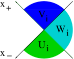
Figure 9: Piece-wise pure-gauge field $\tilde{A}_{i}$.

can be obtained by “squaring” of the propagator in the background of one shock wave (90). In the region $x_{\ast}>0,x_{\bullet}<0$ and $y_{\ast},y_{\bullet}<0$ it is given by Eq, (90) with appropriate substitutions:

$$\langle A_{\mu}(x)A_{\nu}(y)\rangle_{\rm ret}$$ (93)

$$=~{}V_{x}(x|{1\over p^{2}+i\epsilon p_{0}}O_{\mu\nu}(V^{\dagger}W){1\over p^{2}+i\epsilon p_{0}}|y)W^{\dagger}_{y}$$

where

$$O_{\mu\nu}(U)$$ (94)

$$=~{}\!\int\!dz\delta({2\over s}z_{\ast})~{}|z)\Big{\{}2\alpha g_{\mu\nu}V^{\dagger}W+{4i\over s}(p_{2\nu}\partial_{\mu}(V^{\dagger}W)$$

$$+\mu\leftrightarrow\nu)-{4p_{2\mu}p_{2\nu}\over\alpha s^{2}}(\partial_{\perp}^{2}(V^{\dagger}W)+i[U_{i},V^{i}]W)\Big{\}}(z|$$

Here the last term $\sim[U_{i},V^{i}]$ (additional in comparison to Eq. (89)) is due to the source contribution to the second variational derivative of the action

$${\delta^{2}S\over\delta A^{a}_{\mu}(x)\delta A^{b}_{\mu}(y)}$$ (95)

$$=~{}\Big{[}D^{2}g_{\mu\nu}+2iF_{\mu\nu}-{4p_{2\mu}p_{2\nu}\over s^{2}}\Big{\{}{1\over\alpha}\delta({2\over s}x_{\ast})(\partial_{i}$$

$$+~{}i[V_{i})U^{i}+{1\over\beta}\delta({2\over s}x_{\bullet})(\partial_{i}+i[U_{i})V^{i}\Big{\}}\Big{]}^{ab}\delta(x-y)$$

The propagator in the region $x_{\ast}<0,x_{\bullet}>0$ and $y_{\ast},y_{\bullet}<0$ is similar to Eq. (93)

$$\langle A_{\mu}(x)A_{\nu}(y)\rangle_{\rm ret}$$ (96)

$$=~{}U_{x}(x|{1\over p^{2}+i\epsilon p_{0}}\tilde{O}_{\mu\nu}(U^{\dagger}W){1\over p^{2}+i\epsilon p_{0}}|y)W^{\dagger}_{y}$$

where

$$\tilde{O}_{\mu\nu}(U^{\dagger}W)$$ (97)

$$=~{}\!\int\!dz\delta({2\over s}z_{\bullet})~{}|z)\Big{\{}2\beta g_{\mu\nu}U^{\dagger}W+{4i\over s}(p_{2\nu}\partial_{\mu}(U^{\dagger}W)$$

$$+\mu\leftrightarrow\nu)-{4p_{2\mu}p_{2\nu}\over\beta s^{2}}(\partial_{\perp}^{2}(U^{\dagger}W)+i[V_{i},U^{i}]W)\Big{\}}(z|$$

Finally, the propagator at $x_{\ast},x_{\bullet}>0$ and $y_{\ast},y_{\bullet}<0$ has the form:

$$\langle A_{\mu}(x)A_{\nu}(y)\rangle_{\rm ret}$$ (98)

$$=~{}i(x|{1\over p^{2}+i\epsilon p_{0}}\Big{\{}O_{\mu\xi}(U){1\over p^{2}+i\epsilon p_{0}}\tilde{O}^{\xi}_{~{}\nu}(U^{\dagger}W)$$

$$+~{}i\tilde{O}_{\mu\xi}(V){1\over p^{2}+i\epsilon p_{0}}O^{\xi}_{~{}\nu}(V^{\dagger}W)\Big{\}}{1\over p^{2}+i\epsilon p_{0}}|y)W^{\dagger}_{y}$$

Appendix B Pure gauge field $E$ in the second order

From $F_{\mu\nu}(U_{i}+V_{i}+E_{i})=0$ we get

$$(\partial_{i}-i[W_{i},)E_{j}-i\leftrightarrow j~{}=~{}i([U_{i},V_{j}]-i\leftrightarrow j-[E_{i},E_{j}])$$ (99)

If we choose the $(\partial_{i}-i[W_{i},)E^{i}=0$ condition the above equation reduces to the recursion formula

$$E^{a}_{i}~{}=~{}-g(x_{\perp}|W{p^{k}\over p_{\perp}^{2}}W^{\dagger}|^{ab}[U_{i},V_{k}]^{b}-i\leftrightarrow k-g[E_{i},E_{k}]^{b})$$ (100)

It is convenient to introduce complex coordinates in the 2-dimensional plane: $z=z_{1}+iz_{2},\bar{z}=z_{1}-iz_{2}$ and $Q=Q_{1}+iQ_{2},\bar{Q}=Q_{1}-iQ_{2}$ for arbitrary vector $Q$. In these notations the recursion formula (100) simplifies to

$$E^{a}~{}=~{}-g(x_{\perp}|W{i\over\bar{p}}W^{\dagger}|^{ab}K_{12}-E_{12})$$ (101)

where $K_{12}\equiv[U_{1},V_{2}]-[U_{2},V_{1}]$ and $E_{12}\equiv[E_{1},E_{2}]$. In the leading order $W{1\over\bar{p}}W^{\dagger}$ can be approximated by cluster expansion: $W{1\over\bar{p}}W^{\dagger}\simeq\Big{(}{1\over\bar{P}}\Big{)}_{(1)}$ where $\Big{(}{1\over\bar{P}_{(1)}}\Big{)}\equiv U{1\over\bar{p}}U^{\dagger}+V{1\over\bar{p}}V^{\dagger}-{1\over\bar{p}}$ and therefore we get Eq. (34). In the second order we need one more term of the cluster expansion:

$$W{1\over\bar{p}}W^{\dagger}~{}\simeq~{}\Big{(}{1\over\bar{P}_{(1)}}\Big{)}+(U{1\over\bar{p}}U^{\dagger}-{1\over\bar{p}})\bar{p}(V{1\over\bar{p}}V^{\dagger}-{1\over\bar{p}})$$

$$+~{}(U{1\over\bar{p}}U^{\dagger}-{1\over\bar{p}})\bar{p}(V{1\over\bar{p}}V^{\dagger}-{1\over\bar{p}})-\Big{(}{1\over\bar{P}_{(1)}}\Big{)}\bar{E}^{(1)}\Big{(}{1\over\bar{P}_{(1)}}\Big{)}$$

so the second-order expression for $E$ is

$$E^{a(2)}~{}=~{}-ig(x_{\perp}|\Big{(}{1\over P}\Big{)}_{(1)}|^{ab}[E^{1}_{1},E^{1}_{2}]^{b})$$ (102)

$$-~{}ig(x_{\perp}|(U{1\over p}U^{\dagger}-{1\over p})p(V{1\over p}V^{\dagger}-{1\over p})+U\leftrightarrow V|^{ab}K^{b}_{12})$$

Similarly, for the $\bar{E}$ component we get

$$\bar{E}^{a(2)}~{}=~{}ig(x_{\perp}|\Big{(}{1\over{\bar{P}}_{(1)}}\Big{)}|^{ab}[E^{1}_{1},E^{1}_{2}]^{b})$$ (103)

$$+~{}ig(x_{\perp}|(U{1\over{\bar{p}}}U^{\dagger}-{1\over\bar{p}})\bar{p}(V{1\over\bar{p}}V^{\dagger}-{1\over\bar{p}})+U\leftrightarrow V|^{ab}K^{b}_{12})$$

The corresponding formula for the pure gauge field ${\cal E}$ in the left sector is obtained by the trivial replacements $U\rightarrow{\cal U}$ and $V\rightarrow{\cal V}$.

Appendix C Classical fields in the second order

C.1 The fields at $x_{\ast},x_{\bullet}<0$

Figure 10: Classical field in the backwards cone

Since all the Green functions in our expansion are retarded, the only second-order contribution order the classical field $\bar{A}^{(2)}$ is comes from the $D^{k}F_{ik}$ part of the linear term shown in Fig. 10. At $x_{\ast},x_{\bullet}<0$ the gluons in Fig. 10 propagate in the external field $U_{i}+V_{i}$. It is convenient to add (and subtract later) the external field $E_{i}$. The contribution of the diagram in Fig. 10 gives then

$$i\int\!d^{4}z(x|{\theta(-z_{\ast})\theta(-z_{\bullet})\over(P-E)^{2}g_{ik}+2i\bar{G}_{ik}}|z)^{ab}D^{j}L^{b}_{kj}(z)$$

$$=~{}-(x_{\perp}|W{p^{k}\over p_{\perp}^{2}}W^{\dagger}|^{ab}L_{ik}^{b})+2(x_{\perp}|W{p^{k}\over p_{\perp}^{2}}W^{\dagger}|^{ab}[E_{i},E_{k}]^{b})$$

$$\hskip 34.1433pt+~{}(x_{\perp}|W{1\over p_{\perp}^{2}}W^{\dagger}|^{ab}[L_{ik},E^{k}]^{b})$$

Since each of the two legs in the diagram in Fig. 7a represents $E_{i}$ with our accuracy, the Fig. 7a contribution can be reduced to

$$(x_{\perp}|W{1\over p_{\perp}^{2}}W^{\dagger}|^{ab}i[D_{i}E_{k}-i\leftrightarrow k,E^{k}]^{b})$$

$$-~{}(x_{\perp}|W{p^{k}\over p_{\perp}^{2}}W^{\dagger}|^{ab}[E_{i},E_{k}]^{b})$$

Combining these two terms we get (at $x_{\ast},x_{\bullet},0$)

$$A^{a}_{i}(x)~{}=~{}-(x_{\perp}|W{p^{k}\over p_{\perp}^{2}}W^{\dagger}|^{ab}L_{ik}^{b})$$

$$+~{}(x_{\perp}|W{p^{k}\over p_{\perp}^{2}}W^{\dagger}|^{ab}[E_{i},E_{k}]^{b})~{}=~{}E^{a}_{i}(x_{\perp})$$ (104)

up to the terms $\sim[U,V]^{3}$, see Eq. (102). Also, it is easy to see that the longitudinal components $A_{\bullet}$ and $A_{\ast}$ vanish at $x_{\ast},x_{\bullet}<0$.

C.2 The fields at $x_{\ast}>0,x_{\bullet}<0$

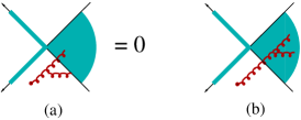
Figure 11: Classical field iat $x_{\ast}>0,x_{\bullet}<0$

First, we note that there are two types of diagrams shown in Fig. 11: with the three-gluon vertex in the $z_{\ast}>0,z_{\bullet}<0$ quadrant and in the $z_{\ast},z_{\bullet}<0$ quadrant. The contribution of the first type (see Fig. 11a) vanishes because the only non-zero component of the first-order field $\bar{A}^{(1)}_{\mu}$ in this case is $\bar{A}^{(1)}_{\bullet}$ such that $D_{\ast}\bar{A}^{(1)}_{\bullet}=0$, see the Eq. (68).

Next we calculate the diagram in Fig. 11b. As in the previous case, the gluon legs are attached only to the $D^{k}F_{ik}$ part of the linear term (27). The gluons in Fig. 11b propagate in the external field $U_{i}\theta(-x_{\ast})+V_{i}\theta(-x_{\bullet})$. The propagator in this background is given by the cluster expansion (91) or, if one needs the $[U,V]^{2}$ accuracy, by Eq. (92) and formulas(93)-(98).

Let us start with the transverse component of the field $A_{i}$. If the three-gluon vertex is integrated over only the $z_{\ast},z_{\bullet}<0$ quadrant one can demonstrate that similarly to the $x_{\ast},x_{\bullet}<0$ case, the contribution of the diagram in Fig. 11b reduces to

$$A^{a}_{i}(x)~{}=~{}\int\!d^{4}z\theta(-z_{\ast})\theta(-z_{\bullet})$$ (105)

$$(x|{1\over\tilde{P}^{2}}\tilde{P}^{k}|z)^{ab}\Big{(}L_{ik}^{b}(z_{\perp})-[E_{i},E_{k}]^{b}(z_{\perp})\Big{)}$$

where $P_{i}=i\partial_{i}+g\tilde{A}_{i}$, $\tilde{A}_{i}=U_{i}\theta(-x_{\ast})+V_{i}\theta(-x_{\bullet})+E_{i}\theta(-x_{\ast})\theta(-x_{\bullet})$. Using the Green function in the the two-shock-wave background (96), we see that the r.h.s. of Eq. (105) vanish so $A_{i}^{(1)}=A_{i}^{(2)}=0$.

It is easy to see that $A_{\ast}=0$ at $x_{\ast}>0,x_{\bullet}<0$ so we are left with $A_{\bullet}$ only. Again, since the only contribution from the three-gluon vertex comes from the $z_{\ast},z_{\bullet}<0$ cone, it can be demonstrated that

$$A^{a}_{\bullet}(x)~{}=~{}-2i\!\int\!d^{4}z\theta(-z_{\ast})\theta(-z_{\bullet})$$ (106)

$$\times~{}(x|{1\over\tilde{P}^{2}}\bar{F}_{\bullet i}{1\over\tilde{P}^{2}}\tilde{P}^{k}|z)^{ab}\Big{(}L_{ik}(z_{\perp})-[E_{i},E_{k}](z_{\perp})\Big{)}^{b}$$

Substituting the explicit form of the Green function (87,88) one obtains

$$-2i\!\int\!d^{4}z\theta(-z_{\ast})\theta(-z_{\bullet})(x|V{1\over p^{2}}V^{\dagger}\bar{F}_{\bullet i}W{p^{k}\over p^{2}}W^{\dagger}|z)^{ab}$$

$$\times~{}\Big{(}L_{ik}(z_{\perp})-[E_{i},E_{k}](z_{\perp})\Big{)}^{b}$$

$$=~{}2(x|V{1\over p^{2}}V^{\dagger}{1\over\alpha-i\epsilon}|^{ab}0,[U_{i},E^{i}]^{b})\delta({2\over s}x_{\ast})$$

Thus, the only non-vanishing component of the classical filed in the $x_{\ast}\geq 0,x_{\bullet}<0$ region is

$$A^{a}_{\bullet}(x)~{}=~{}-2i\delta({2\over s}x_{\ast})(x_{\perp}|V{1\over p_{\perp}^{2}}V^{\dagger}|^{ab}[U_{i},E^{i}]^{b})$$ (107)

Similarly, at $x_{\ast}<0,x_{\bullet}\geq 0$

$$A^{a}_{\bullet}(x)~{}=~{}-2i\delta({2\over s}x_{\bullet})(x_{\perp}|U{1\over p_{\perp}^{2}}U^{\dagger}|^{ab}[V_{i},E^{i}]^{b})$$ (108)

C.3 The fields in the forward cone $x_{\ast},x_{\bullet}>0$

C.3.1 The three-gluon vertex in the backward cone

At first, we consider the contribution from Fig. 7a where the three-gluon vertex integrated over $z_{\ast},z_{\bullet}<0$ quadrant. This contribution is similar to the one we considered in the previous section so we can start with the expressions (105) and (106). Using the Green functions in the $\tilde{A}$ background given by Eq. (92) and formulas (93)-(98), one obtains

$$\bar{A}_{\mu}^{a}(x)=\int\!d^{4}z(x|{1\over p^{2}+i\epsilon p_{0}}\Big{\{}2|0,E^{a}_{\perp\mu})$$ (109)

$$+~{}{4\over s}\Big{(}{p_{1\mu}p_{\perp}^{2}\over\beta-i\epsilon}U+is\partial_{\mu}U-{p_{2\mu}\partial_{\perp}^{2}U\over\alpha+i\epsilon}\Big{)}{1\over p_{\perp}^{2}}U^{\dagger}|^{ab}0,[V_{i},E^{i}]^{b})$$

$$+~{}{4\over s}\Big{(}{p_{2\mu}p_{\perp}^{2}\over\beta-i\epsilon}V+is\partial_{\mu}V-{p_{1\mu}\partial_{\perp}^{2}V\over\alpha+i\epsilon}\Big{)}{1\over p_{\perp}^{2}}V^{\dagger}|^{ab}0,[U_{i},E^{i}]^{b})$$

C.3.2 First part of the Lipatov vertex

The sum of all the contributions calculated up to now (which includes everything but the terms with three-gluon vertex outside the backward cone) can be rewitten in the form of Eq. (VII.2)

$${\bar{A}}_{i}^{{\rm 1st}}~{}=~{}\theta(-x_{\ast})\theta(-x_{\bullet})W_{i}(x_{\perp})+~{}\theta(-x_{\ast})\theta(x_{\bullet})U_{i}(x_{\perp})$$

$$+~{}\theta(x_{\ast})\theta(-x_{\bullet})V_{i}(x_{\perp})+(x|{1\over p^{2}+i\epsilon p_{0}}|R^{\rm(1)}_{\mu}+\delta R^{\rm(2)}_{\mu})$$

where $R^{\rm(1)}_{\mu}(p)$ is given by Eq. (77)

$$R^{\rm(1)}_{\mu}(p)~{}=~{}R^{\rm(1)}_{\perp\mu}(p_{\perp})+{2p_{1\mu}\over s}\Big{(}{R_{1+}^{\rm(1)}(p_{\perp})\over\beta+i\epsilon}+{R_{1-}^{\rm(1)}(p_{\perp})\over\beta-i\epsilon}\Big{)}$$

$$+~{}{2p_{2\mu}\over s}\Big{(}{R_{2+}^{\rm(1)}(p_{\perp})\over\alpha+i\epsilon}+{R_{2-}^{\rm(1)}(p_{\perp})\over\alpha-i\epsilon}\Big{)}$$ (110)

and the last term

$$\delta R^{\rm(2)}_{\mu}(k) = {4p_{1\mu}\over s(\beta+i\epsilon)}([U_{i},V^{i}]V{1\over p_{\perp}^{2}}V^{\dagger}U_{j})^{ab}E^{jb}$$ (111)

$$- {4p_{2\mu}\over s(\alpha+i\epsilon)}([U_{i},V^{i}]U{1\over p_{\perp}^{2}}U^{\dagger}V_{j})^{ab}E^{jb}$$

is actually a part of the second-order contribution coming from the $[U_{i},V^{i}]$ term in the Green function (see Eq. (94).

The remaining part of the Lipatov vertex (coming from the diagram Fig. 2b with $z$ outside the backward cone) will have the same structure (77) with different $R_{\perp},R_{1}$, and $R_{2}$. Note that our first part of Lipatov vertex (77) satisfies the condition

$$p^{\mu}R^{\rm(1)}_{\mu}(p)=p^{i}R^{\rm(1)}_{i}+R^{\rm(1)}_{1+}+R^{\rm(1)}_{1-}+R^{\rm(1)}_{2+}+R^{\rm(1)}_{2-}=0$$ (112)

(recall that $(i\partial_{i}+g[U_{i}+V_{i},)E^{i}=0$).

C.3.3 The three-gluon vertex outside the backward cone

Here we must calculate the diagram in Fig. 2b with three-gluon vertex outside the backward cone $x_{\ast},x_{\bullet}<0$. With our accuracy, each of the two legs in Fig. 2b can be represented by the field

$$\bar{A}^{1}_{\mu}~{}=~{}(x|{1\over p^{2}+i\epsilon p_{0}}|R^{(1)}_{\mu})$$ (113)

so we get

$$\bar{A}^{(2)}_{\mu} = i\int d^{4}z(x|(P^{2}g_{\mu\alpha}+2iF_{\mu\alpha}+i\epsilon p_{0})^{-1}|z)^{ab}$$ (114)

$$\times ~{}[\bar{A}^{(1)\beta},D_{\alpha}\bar{A}^{(1)}_{\beta}-2D_{\beta}\bar{A}^{(1)}_{\alpha}]^{b}(z)$$

where we have used the gauge condition $D^{\mu}\bar{A}^{(1)}_{\mu}=0$ .

It is easy to see that the term $\sim G_{\mu\alpha}$ in the above equation can be dropped. Indeed, since the point $z$ lies outside the backward cone, the only non-vanishing contribution proportional to, say, $F_{\bullet i}$ can come from the quadrant $z_{\ast}\leq 0,z_{\bullet}\geq 0$ where the only surviving component of the field is $\bar{A}^{(1)}_{\ast}=-i\delta(x_{\bullet})(x_{\perp}|{1\over p_{\perp}^{2}}|[V_{i},E^{i}])$. (see eq. (68)). In addition, $D_{\bullet}\bar{A}^{(1)}_{\ast}=0$ and therefore all possible terms $\sim G_{\mu\alpha}$ in r.h.s. of Eq. (114) vanish and therefore

$$\bar{A}^{(2)}_{\mu}(x)~{}=$$ (115)

$$i\!\int\!d^{4}z(x|{1\over P^{2}+i\epsilon p_{0}}|z)^{ab}[\bar{A}^{(1)\nu},D_{\mu}\bar{A}^{(1)}_{\nu}-2D_{\nu}\bar{Q}^{(1)}_{\mu}]^{b}(z)$$

For the same reason, the Green function ${1\over P^{2}+i\epsilon p_{0}}$ in r.h.s. of Eq. (115) can be replaced by bare propagator ${1\over p^{2}+i\epsilon p_{0}}$. Indeed, these expressions differ only outside the forward cone which means either $z_{\ast}<0,z_{\bullet}\geq 0$ or $z_{\ast}\geq 0,z_{\bullet}<0$ quadrants (recall that we exclude the backward cone $z_{\ast},z_{\bullet}<0$). Consider the contribution to r.h.s. (115) coming from $z_{\ast}<0,z_{\bullet}\geq 0$ quadrant. The only nonzero component of the field $A_{\mu}$ in this quadrant is $A_{\bullet}$ (see above) and since $D_{\ast}A_{\bullet}=0$ the r.h.s. of Eq. (115) vanishes.

We get

$$\bar{A}^{(2)}_{\mu}(x)~{}=$$ (116)

$$i\!\int\!d^{4}z(x|{1\over p^{2}+i\epsilon p_{0}}|z)^{ab}[\bar{A}^{(1)\nu},\partial_{\mu}\bar{A}^{(1)}_{\nu}-2\partial_{\nu}\bar{A}^{(1)}_{\mu}]^{b}(z)$$

The Lipatov vertex is represented by the two terms in square brackets. We will calculate them in turn.

The contribution to Lipatov vertex from the first term is

$$R^{\rm(2)}_{\mu(1)}(k)~{}=~{}i\!\int\!d^{4}z~{}e^{ikz}[\bar{A}^{(1)\nu},\partial_{\mu}\bar{A}^{(1)}_{\nu}](z)$$ (117)

First, let us calculate the part of this integral coming from the product of two $R^{(1)}_{\perp}$ terms. We have

$$R^{\rm(2)}_{\mu(11)}(k)~{}=\int\!{d^{4}k^{\prime}\over 16\pi^{4}}{(k-k^{\prime})_{\mu}[R_{\perp}^{(1)i}(k^{\prime}_{\perp}),R^{(1)}_{\perp i}(k-k^{\prime}_{\perp})]\over({k^{\prime}}^{2}+i\epsilon k^{\prime}_{0})[(k-k^{\prime})^{2}+i\epsilon(k-k^{\prime})_{0}]}$$

$$=~{}{i\over 2}\!\int\!{d^{2}k^{\prime}_{\perp}\over 16\pi^{3}}\!\int_{-\infty}^{\infty}\!du~{}{(1-2u)(\alpha p_{1}+\beta p_{2})_{\mu}+(k-2k^{\prime})^{\perp}_{\mu}\over(k^{\prime}-ku)^{2}-(k^{2}+i\epsilon k_{0})\bar{u}u}$$

$$\hskip 93.89409pt\times~{}[R_{\perp}^{(1)i}(k^{\prime}_{\perp}),R^{(1)}_{\perp i}(k-k^{\prime}_{\perp})]$$

$$=~{}-{1\over 2}f^{abc}\!\int\!{d^{2}k^{\prime}_{\perp}\over 16\pi^{2}}{1\over\sqrt{\cal G}}[R_{\perp}^{(1)i}(k^{\prime}_{\perp}),R^{(1)}_{\perp i}(k-k^{\prime}_{\perp})]$$

$$\hskip 8.53581pt\times~{}\Big{\{}\Big{(}{p_{1}\over\beta s}+{p_{2}\over\alpha s}\Big{)}(k,k-2k^{\prime})_{\perp}+(k-2k^{\prime})^{\perp}\Big{\}}_{\mu}$$ (118)

Note that $k^{\mu}R^{\rm(2)}_{\mu(11)}(k)~{}=~{}0$.

The second part of $R^{\rm(2)}_{\mu(1)}$ is easlily calculated using formulas from Appendix D with the result

$$R^{\rm(2)~{}a}_{\mu(12)}(k)$$

$$=~{}f^{abc}\!\int\!{d^{2}k^{\prime}_{\perp}\over 16\pi^{3}}\!\int_{-\infty}^{\infty}\!{du\over Z(u)}~{}\Big{(}{-2p_{1\mu}\over s(\beta u+i\epsilon)}+~{}{2p_{2\mu}\over s(\alpha\bar{u}+i\epsilon)}$$

$$+~{}{\bar{u}(\alpha p_{1}-\beta p_{2}-k_{\perp}+2k^{\prime}_{\perp})_{\mu}\over(k-k^{\prime})_{\perp}^{2}(u+i\epsilon)}\Big{)}R^{\rm(1)}_{1b}(k^{\prime}_{\perp})R^{\rm(1)}_{2c}(k_{\perp}-k^{\prime}_{\perp})$$

$$+~{}{4p_{1\mu}\over s(\beta+i\epsilon)}([U_{i},V^{i}]U{1\over p_{\perp}^{2}}U^{\dagger})^{ab}[V_{j},E^{j}]^{b}$$

$$-~{}{4p_{2\mu}\over s(\alpha+i\epsilon)}([U_{i},V^{i}]V{1\over p_{\perp}^{2}}V^{\dagger})^{ab}[U_{j},E^{j}]^{b}$$ (119)

where $Z(u)=(k^{\prime}-ku)_{\perp}^{2}-(k^{2}+i\epsilon k_{0})\bar{u}u$ and $R^{\rm(1)}_{1}\equiv R^{\rm(1)}_{1+}+R^{\rm(1)}_{1-}$, $R^{\rm(1)}_{2}\equiv R^{\rm(1)}_{2+}+R^{\rm(1)}_{2-}$

The remaining third part of the second-order term is

$$R^{\rm(2)}_{\mu(1)}(k)~{}=~{}-2i\!\int\!d^{4}z~{}e^{ikz}[\bar{Q}^{(1)\nu},\partial_{\nu}\bar{Q}^{(1)}_{\mu}](z)$$

$$=~{}f^{abc}\!\int\!{d^{2}k^{\prime}_{\perp}\over 16\pi^{3}}\!\int_{-\infty}^{\infty}\!{du\over Z(u)}~{}\Bigg{[}-~{}4{\bar{u}(\alpha p_{1}-\beta p_{2})_{\mu}\over(k-k^{\prime})_{\perp}^{2}(u+i\epsilon)}$$

$$\times~{}R^{\rm(1)}_{1b}(k^{\prime}_{\perp})R^{\rm(1)}_{2c}(k_{\perp}-k^{\prime}_{\perp})$$

$$+~{}2(k_{i}g_{\mu j}-i\leftrightarrow j)R^{\rm(1)}_{ib}(k^{\prime}_{\perp})R^{\rm(1)}_{jc}(k_{\perp}-k^{\prime}_{\perp})\Bigg{]}$$ (120)

Combining Eqs. (118), (119), and (120) we get the total second-order term

$$R^{\rm(2)~{}a}_{\mu}(k)$$

$$=~{}if^{abc}\!\int\!{d^{2}k^{\prime}_{\perp}\over 16\pi^{3}}\!\int_{-\infty}^{\infty}\!{du\over Z(u)}~{}\Bigg{[}\Big{(}(1-2u)(\alpha p_{1}+\beta p_{2})_{\mu}$$

$$+~{}(k-2k^{\prime})^{\perp}_{\mu}\Big{)}R^{\rm(1)~{}b}_{\perp i}(k^{\prime}_{\perp})R^{\rm(1)~{}c~{}i}_{\perp}(k_{\perp}-k^{\prime}_{\perp})$$

$$+~{}\Big{(}{-2p_{1\mu}\over s(\beta u+i\epsilon)}+~{}{2p_{2\mu}\over s(\alpha\bar{u}+i\epsilon)}$$

$$+~{}{\bar{u}(\alpha p_{1}-\beta p_{2}-k_{\perp}+2k^{\prime}_{\perp})_{\mu}\over(k-k^{\prime})_{\perp}^{2}(u+i\epsilon)}\Big{)}R^{\rm(1)}_{1b}(k^{\prime}_{\perp})R^{\rm(1)}_{2c}(k_{\perp}-k^{\prime}_{\perp})$$

$$+~{}2(k_{i}g_{\mu j}-i\leftrightarrow j)R^{\rm(1)}_{ib}(k^{\prime}_{\perp})R^{\rm(1)}_{jc}(k_{\perp}-k^{\prime}_{\perp})\Bigg{]}$$

$$+~{}{4\over s}\Big{(}{p_{1\mu}\over\beta+i\epsilon}-~{}{p_{2\mu}\over\alpha+i\epsilon}\Big{)}\Big{(}[U_{i},V^{i}]U{1\over p_{\perp}^{2}}U^{\dagger})^{ab}[V_{j},E^{j}]^{b}$$

$$+~{}([U_{i},V^{i}]V{1\over p_{\perp}^{2}}V^{\dagger})^{ab}[U_{j},E^{j}]^{b}\Big{)}$$ (121)

The integral over $u$ yields Eq. (79).

Appendix D Gluon emission by two Wilson lines in the shock-wave background

D.1 Classical field induced by a single Wilson line in the shock-wave background

In the applications it is sometimes convenient to have the result for the classical field and the Lipatov vertex in a “non-symmetric” form explicitly expanded over the strength of the weak source $\sim{\rm Tr}\{\rho(x_{\perp})U(x_{\perp})\}$. This expansion corresponds to the diagrams with a gluon production by Wilson lines $\parallel p_{1}$ in the background of the shock wave. In this case it more convenient to present the results for the covariant gauge shock field $A_{\bullet}\sim\delta(x_{\ast})$. (The rotation to the pure-gauge field $U_{i}\theta(-x_{\ast})$ is trivial).

In the first order the classical field is given by the two diagrams in Fig.12

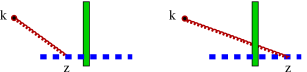
Figure 12: Emission of a gluon by a Wilson line in the shock-wave background.

As in Sect. VII we consider here the case of the causal classical field corresponding to ${\cal U}=U$ which is the case when we neglect the evolution. Note it is not difficult to restore the result for ${\cal U}\neq U$ similarly to Eq. (38) - roughly speaking, one should replace $(p^{2}+i\epsilon p_{0})^{-1}U$ by $(p^{2}+i\epsilon)^{-1}U+2\pi i\delta(p^{2})\theta(p_{0}){\cal U}$.

The expression for the classical field produced by one Wilson-line source can be read from the (retarded) propagator in a shock-wave background (90). At $x_{\ast}>0$ one gets

$$i\langle A^{\mu}(k)[\infty p_{1},-\infty p_{1}]_{z}\rangle_{\rm ret}~{}=~{}{1\over k^{2}+i\epsilon k_{0}}R^{\mu}_{V}(k),$$ (122)

$$R_{V}^{a\mu}(k)~{}=~{}(k|\Big{\{}2i\partial^{\mu}U{1\over p_{\perp}^{2}}+p_{1}^{\mu}\Big{(}2\alpha U{1\over p_{\perp}^{2}}$$

$$-~{}{2\over s(\beta+i\epsilon)}U\Big{)}-{2p_{2}^{\mu}\over\alpha s}\partial_{\perp}^{2}U{1\over p_{\perp}^{2}}\Big{\}}|0,z_{\perp})^{ab}U_{z}t^{b}$$

The emission of gluon by the c.c. Wilson line $V^{\dagger}=[-\infty p_{1},\infty p_{1}]_{z}$ differs from Eq. (122) by sign and the replacement $t^{b}U\leftrightarrow U^{\dagger}t^{b}$:

$$i\langle A^{\mu}(k)[-\infty p_{1},\infty p_{1}]_{z}\rangle_{\rm ret}~{}=~{}{1\over k^{2}+i\epsilon k_{0}}R^{\mu}_{V}(k),$$ (123)

$$R_{V\dagger}^{a\mu}(k)~{}=~{}-(k|\Big{\{}2i\partial^{\mu}U{1\over p_{\perp}^{2}}+p_{1}^{\mu}\Big{(}2\alpha U{1\over p_{\perp}^{2}}$$

$$-~{}{2\over s(\beta+i\epsilon)}U\Big{)}-{2p_{2}^{\mu}\over\alpha s}\partial_{\perp}^{2}U{1\over p_{\perp}^{2}}\Big{\}}|0,z_{\perp})^{ab}t^{b}U^{\dagger}_{z}$$

The (transverse) Lipatov vertices in the light-like gauge are obtained from Eq. (41):

$$L^{(1)}_{Vi}(k_{\perp};z_{\perp})~{}=~{}2(k_{\perp}|\big{[}{p_{i}\over p_{\perp}^{2}},U\big{]}|0,z_{\perp})^{ab}U_{z}t^{b}$$ (124)

$$L^{(1)}_{V^{\dagger}i}(k_{\perp};z_{\perp})~{}=~{}-2(k_{\perp}|\big{[}{p_{i}\over p_{\perp}^{2}},U\big{]}|0,z_{\perp})^{ab}t^{b}U^{\dagger}_{z}$$

Note that the fields in this Section are presented in the bF gauge in the background of one shock wave $U$ which differs from the bF gauge for the background field $U_{i}+V_{i}$ used in the bulk of the paper. However, the final result (124) for the Lipatov vertex $L_{i}$ corresponds to the $p_{2}^{\mu}A_{\mu}=0$ gauge and therefore agrees with Eq. (73). Indeed, in Sect. VI it was shown that at small $V_{i}$ Eq. (73) reduces to

$$L^{(1)}_{i}(k)~{}=~{}2(k|\big{[}{p_{i}\over p_{\perp}^{2}},U\big{]}p^{k}U^{\dagger}|^{ab}0,V_{k}^{b})$$ (125)

which agrees with Eq. (124) if one uses the formula $V_{x}V^{\dagger}_{y}=P\exp ig\int_{x}^{y}dx^{i}V_{i}$ for $V(z_{\perp})=[\infty p_{1}+z_{\perp},-\infty p_{1}+z_{\perp}]$ as in Sect. VI.

D.2 Classical field and the Lipatov vertex due to the two Wilson lines

In the second order, the field due to two Wilson lines is given by the diagrams shown in Fig. 13. These diagrams are calculated using the retarded Green function (90) integrated with the three-gluon vertex. The calculation is similar to that of Appendix C and the result has the form (the details of the calculation will be published elsewhere):

$$\langle A^{\mu}(k)[\infty,-\infty]_{z}[-\infty,\infty p_{1}]_{z^{\prime}}\rangle_{\rm ret}~{}=~{}{R^{(2)\mu}_{VV^{\dagger}}(k)\over k^{2}+i\epsilon k_{0}}$$

$$R^{(2)a\mu}_{VV^{\dagger}}(k)~{}=~{}f^{abc}\!\int\!{d^{2}k^{\prime}_{\perp}\over 8\pi^{2}}$$

$$\Bigg{\{}{1\over\sqrt{\cal G}}\Big{(}k^{\xi}\delta_{\mu}^{\eta}-k^{\eta}\delta_{\mu}^{\xi}-{K_{\mu}\over 2}g^{\xi\eta}\Big{)}\tilde{R}_{V_{\xi}}^{b}(k^{\prime}_{\perp})\tilde{R}_{V^{\dagger}\eta}^{c}(k_{\perp}-k^{\prime}_{\perp})$$

$$+~{}2i\Big{(}{p_{2}\over\alpha s}-{p_{1}\over\beta s}\Big{)}_{\mu}\Big{[}{(k^{\prime},k-k^{\prime})_{\perp}+{k^{2}\over 2}-i\sqrt{\cal G}\over{k^{\prime}}_{\perp}^{2}(k-k^{\prime})_{\perp}^{2}}$$

$$\times~{}\Big{(}R_{1V}^{b}(k^{\prime}_{\perp};z_{\perp})R_{2V^{\dagger}}^{c}(k_{\perp}-k^{\prime}_{\perp};z^{\prime}_{\perp})-R_{2V}^{b}(k^{\prime}_{\perp};z_{\perp})$$

$$\times~{}R_{1V^{\dagger}}^{c}(k_{\perp}-k^{\prime}_{\perp};z^{\prime}_{\perp})\Big{)}-R^{b}_{2V}(k^{\prime};z_{\perp})$$

$$\times~{}r^{c}_{V^{\dagger}}(k_{\perp}-k^{\prime}_{\perp};z^{\prime}_{\perp})+r^{b}_{V}(k^{\prime};z_{\perp})R_{2V^{\dagger}}(k-k^{\prime};z^{\prime})\Big{]}$$

$$-~{}2i(g_{\mu\xi}-2{p_{1\mu}k_{\xi}\over\beta s})\Big{[}r^{b\xi}_{V}(k^{\prime};z_{\perp}))r^{c}_{V^{\dagger}}(k_{\perp}-k^{\prime}_{\perp};z^{\prime}_{\perp})$$

$$-~{}r^{b}_{V}(k^{\prime};z_{\perp}))r^{c\xi}_{V^{\dagger}}(k_{\perp}-k^{\prime}_{\perp};z^{\prime}_{\perp})\Big{]}\Bigg{\}}$$ (126)

where $K_{\mu}$ is given by Eq. (80), and

$$R_{1V}^{a}(k^{\prime}_{\perp};z_{\perp})~{}=~{}(k^{\prime}_{\perp}|[p_{\perp}^{2},U]{1\over p_{\perp}^{2}}|z_{\perp})^{ab}U_{z}t^{b}$$

$$R_{2V}^{a}(k^{\prime}_{\perp};z_{\perp})~{}=~{}-(k^{\prime}_{\perp}|\partial_{\perp}^{2}U{1\over p_{\perp}^{2}}|z_{\perp})^{ab}U_{z}t^{b}$$

$$r_{V}^{a}(k^{\prime}_{\perp};z_{\perp})~{}=~{}(k^{\prime}_{\perp}|U{1\over p_{\perp}^{2}}|z_{\perp})^{ab}U_{z}t^{b}$$

$$r_{V}^{b\xi}(k^{\prime}_{\perp};z_{\perp})~{}=~{}(k^{\prime}_{\perp}|i\partial^{\xi}U{1\over p_{\perp}^{2}}|z_{\perp})^{bm}U_{z}t^{m}$$ (127)

$$\tilde{R}_{V}^{\xi}(k^{\prime}_{\perp};z_{\perp})~{}=~{}\Big{(}2r_{V}^{\xi}(k^{\prime}_{\perp};z_{\perp})+{(k,k^{\prime})_{\perp}+{k^{2}\over 2}-i\sqrt{\cal G}\over{k^{\prime}}_{\perp}^{2}}$$

$$\times~{}\Big{[}{2p_{1}\over\beta s}R_{V1}(k^{\prime}_{\perp};z_{\perp})+{2p_{2}\over\alpha s}R_{V2}(k^{\prime}_{\perp};z_{\perp})\Big{]}_{\xi}\Big{)}^{ab}U_{z}t^{b}$$ (128)

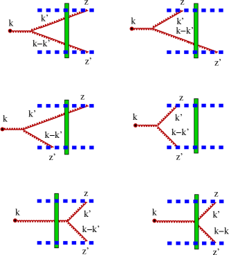
Figure 13: Gluon emission by two Wilson lines.

The corresponding quantities $R_{V^{\dagger}}$ and $r_{V^{\dagger}}$ are obtained by substitution $U_{z}t^{b}\rightarrow t^{b}U^{\dagger}_{z}$:

$$R_{1V^{\dagger}}^{a}(k^{\prime}_{\perp};z_{\perp})~{}=~{}(k^{\prime}_{\perp}|[p_{\perp}^{2},U]{1\over p_{\perp}^{2}}|z_{\perp})^{ab}t^{b}U_{z}^{\dagger}$$

$$R_{2V^{\dagger}}^{a}(k^{\prime}_{\perp};z_{\perp})~{}=~{}-(k^{\prime}_{\perp}|\partial_{\perp}^{2}U{1\over p_{\perp}^{2}}|z_{\perp})^{ab}t^{b}U_{z}^{\dagger}$$

$$r_{V^{\dagger}}^{a}(k^{\prime}_{\perp};z_{\perp})~{}=~{}(k^{\prime}_{\perp}|U{1\over p_{\perp}^{2}}|z_{\perp})^{ab}t^{b}U_{z}^{\dagger}$$

$$r_{V^{\dagger}}^{b\xi}(k^{\prime}_{\perp};z_{\perp})~{}=~{}(k^{\prime}_{\perp}|i\partial^{\xi}U{1\over p_{\perp}^{2}}|z_{\perp})^{bm}t^{m}U_{z}^{\dagger}$$ (129)

and

$$\tilde{R}_{V}^{\xi}(k^{\prime}_{\perp};z_{\perp})~{}=~{}\Big{(}2r_{V}^{\xi}(k^{\prime}_{\perp};z_{\perp})+{(k,k^{\prime})_{\perp}+{k^{2}\over 2}-i\sqrt{\cal G}\over{k^{\prime}}_{\perp}^{2}}$$

$$\times~{}\Big{[}{2p_{1}\over\beta s}R_{V1}(k^{\prime}_{\perp};z_{\perp})+{2p_{2}\over\alpha s}R_{V2}(k^{\prime}_{\perp};z_{\perp})\Big{]}_{\xi}\Big{)}^{ab}U_{z}t^{b}$$ (130)

Note that $Ut^{a}$ and $t^{b}U^{\dagger}$ carry the independent indices of the Wilson lines $[\infty p_{1},-\infty p_{1}]$ and $[-\infty p_{1},\infty p_{1}]$ We do not display the color indices of $U_{z}t^{b}$ and $t^{b}U^{\dagger}_{z}$ - they are always assumed, like $(...)(U_{z}t^{b})^{i}_{j}(...)(t^{b}U^{\dagger}_{z})^{k}_{l}$. Also, the formula (126) will hold true for Wilson lines in the fundamental representation provided one replaces $(Ut^{b})^{i}_{j}$ by $(T^{b}U)^{mn}$ and $(t^{b}U^{\dagger}_{z})^{k}_{l}$ by $(T^{b}U)^{\dagger mn}$.

There is a subtle point in the calculation of diagrams in Fig. 13 related to the existence of a term with gluon vertex inside the shock wave. Consider, for example, the first diagram in Fig. 13. Similarly to Sect. C.3.3, we calculate the integral over $\beta^{\prime}$ (the $p_{2}$ component of vector $k^{\prime}$) by taking residues. However, the integral over $\beta^{\prime}$ becomes divergent if one takes the term $\sim\beta^{\prime}$ in the three-gluon vertex. To deal with such divergence, we must retrace one step back and write down the classical field $\bar{A}^{(2)}$ in the form (114)

$$\bar{A}^{(2)}_{\mu} = i{2p_{2\mu}\over s}\!\int\!d^{y}(k|{1\over P^{2}+i\epsilon p_{0}}|y)^{ab}$$ (131)

$$\times ~{}[\bar{A}^{(1)\beta},D_{\bullet}\bar{A}^{(1)}_{\beta}-2D_{\beta}\bar{A}^{(1)}_{\bullet}]^{b}(z)$$

By the equations of motion, one can replace $D_{\bullet}\bar{A}^{(1)}_{\beta}$ in the r.h.s. of this equation

$$P_{\bullet}\bar{A}^{(1)}_{\beta}~{}\rightarrow~{}{p_{\perp}^{2}\over 2\alpha^{\prime}s}\bar{A}^{(1)}_{\beta}+{2i\over\alpha^{\prime}s}\bar{G}_{\bullet\beta}\bar{A}^{(1)}_{\ast}$$ (132)

The first term in the r.h.s. of this equation does not produce any divergency in $\beta^{\prime}$ and can be calculated by taking residues. The second term is a contribution with the point y (position of the three-gluon vertex) inside the shock wave as shown on the last diagram in Fig. (13). Such terms with the three-gluon vertex inside the shock wave are calculated using the formulas for the propagator with the initial (or final) points in the shock wave:

$$(y|{1\over P^{2}+i\epsilon p_{0}}|z)~{}=~{}[y_{\ast},-\infty]_{y}(y|{1\over p^{2}+i\epsilon p_{0}}|z)$$

$$(k|{1\over P^{2}+i\epsilon p_{0}}|y)~{}=~{}[\infty,y_{\ast}]_{y_{\perp}}(k|{1\over p^{2}+i\epsilon p_{0}}|y)$$ (133)

Summarising, $\beta^{\prime}$ in the three-gluon vertex must be replaced by ${{k^{\prime}}_{\perp}^{2}\over\alpha^{\prime}s}$, $\beta-\beta^{\prime}$ by ${(k-k^{\prime})_{\perp}^{2}\over(\alpha-\alpha^{\prime}s)}$, and t the difference must be taken into account as the term with the gluon vertex inside the shock wave. It is worth noting that the contribution of the last diagram in Fig. 13 (with the gluon vertex inside the shock wave) is essential for the gauge invariance of the Lipatov vertex (cf. ref. saclay2 ).

The classical field due to the two Wilson lines $[\infty p_{1},-\infty p_{1}]_{z}~{}[\infty p_{1},-\infty p_{1}]_{z^{\prime}}$ is proportional to $R^{(2)}_{VV}(k_{\perp};z_{\perp},z^{\prime}_{\perp})$ obtained from (126) by change of sign and the replacement $R_{V^{\dagger}}(k-k^{\prime})^{c}\rightarrow R_{V^{\dagger}}(k_{\perp}-k^{\prime}_{\perp})^{c}$, $r_{V^{\dagger}}(k_{\perp}-k^{\prime}_{\perp})^{c}\rightarrow r_{V^{\dagger}}(k_{\perp}-k^{\prime}_{\perp})^{c}$. Similarly, $R^{(2)}_{V^{\dagger}V^{\dagger}}(k_{\perp};z_{\perp},z^{\prime}_{\perp})$ for the classical field due to $[-\infty p_{1},\infty p_{1}]_{z}~{}[-\infty p_{1},\infty p_{1}]_{z^{\prime}}$ is obtained from (126) by change of sign and the replacement $R_{V}^{b}(k^{\prime}_{\perp})\rightarrow R_{V^{\dagger}}^{b}(k^{\prime}_{\perp})$, $r_{V}^{b}(k^{\prime}_{\perp})\rightarrow r^{b}_{V^{\dagger}}(k^{\prime}_{\perp})$. The Lipatov vertex in the $p_{2}^{\mu}A_{\mu}=0$ gauge takes the form:

$$\Big{(}L^{(2)}_{VV^{\dagger}}(k_{\perp};z_{\perp},z^{\prime}_{\perp})\Big{)}^{a}_{i}~{}=~{}\lim_{k^{2}\rightarrow 0}k^{2}\langle A^{a}_{i}(k)[\infty p_{1},-\infty p_{1}]_{z}~{}[-\infty p_{1},\infty p_{1}]_{z^{\prime}}\rangle_{\rm ret}$$ (134)

$$=~{}gf^{abc}\!\int\!{d^{2}k^{\prime}_{\perp}\over 8\pi^{2}}\Bigg{(}{1\over\sqrt{k_{\perp}^{2}{k^{\prime}}_{\perp}^{2}-(k,k^{\prime})_{\perp}^{2}}}\Bigg{\{}\big{(}k^{\prime}_{i}-k_{i}{(k,k^{\prime})_{\perp}\over k_{\perp}^{2}}\big{)}L^{(1)b}_{Vj}(k^{\prime}_{\perp};z_{\perp})L^{(1)cj}_{V^{\dagger}}(k-k^{\prime}_{\perp};z^{\prime}_{\perp})$$

$$+~{}\Big{[}\Big{(}k_{j}-k^{\prime}_{j}{(k,k^{\prime})_{\perp}\over{k^{\prime}}_{\perp}^{2}}\Big{)}g_{il}-g_{ij}\Big{(}k_{l}-(k-k^{\prime})_{l}{(k,k-k^{\prime})_{\perp}\over(k-k^{\prime})_{\perp}^{2}}\Big{)}\Big{]}L^{(1)bj}_{V}(k^{\prime}_{\perp};z_{\perp})L^{(1)cl}_{V^{\dagger}i}(k-k^{\prime}_{\perp};z^{\prime}_{\perp})\Bigg{\}}$$

$$+~{}i\Bigg{\{}\Big{(}g_{il}{k^{\prime}_{j}\over{k^{\prime}}_{\perp}^{2}}-g_{ij}{(k-k^{\prime})_{l}\over(k-k^{\prime})_{\perp}^{2}}\Big{)}L^{(1)bj}_{V}(k^{\prime}_{\perp};z_{\perp})L^{(1)cl}_{V^{\dagger}i}(k-k^{\prime}_{\perp};z^{\prime}_{\perp})$$

$$-~{}{2\over{k^{\prime}}_{\perp}^{2}}\Big{(}g_{ij}+{k_{i}k^{\prime}_{j}\over k_{\perp}^{2}}\Big{)}R^{b}_{1V}(k^{\prime}_{\perp};z_{\perp})L^{(1)cj}_{V^{\dagger}}(k-k^{\prime}_{\perp};z^{\prime}_{\perp})+{2\over(k-k^{\prime})_{\perp}^{2}}\Big{(}g_{ij}+{k_{i}(k-k^{\prime})_{j}\over k_{\perp}^{2}}\Big{)}L^{(1)bj}_{V}(k^{\prime}_{\perp};z_{\perp})R^{c}_{1V^{\dagger}}(k-k^{\prime}_{\perp};z^{\prime}_{\perp})$$

$$-~{}4{k^{\prime}_{i}k_{\perp}^{2}-k_{i}(k,k^{\prime})_{\perp}\over k_{\perp}^{2}{k^{\prime}}_{\perp}^{2}(k-k^{\prime})_{\perp}^{2}}R^{b}_{1V}(k^{\prime}_{\perp};z_{\perp})R^{c}_{1V^{\dagger}}(k-k^{\prime}_{\perp};z^{\prime}_{\perp})-2\Big{[}{k_{i}\over k_{\perp}^{2}}R^{b}_{2V}(k^{\prime}_{\perp};z_{\perp})+\Big{(}g_{il}+2{k_{i}k^{\prime}_{l}\over k_{\perp}^{2}}\Big{)}r^{bl}_{1V}(k^{\prime}_{\perp};z_{\perp})\Big{]}r^{c}_{V^{\dagger}}(k-k^{\prime}_{\perp};z^{\prime}_{\perp})$$

$$+~{}2r^{b}_{V}(k^{\prime}_{\perp};z_{\perp})\Big{[}{k_{i}\over k_{\perp}^{2}}R^{c}_{2V^{\dagger}}(k-k^{\prime}_{\perp};z_{\perp})+\Big{(}g_{il}+2{k_{i}(k-k^{\prime})_{l}\over k_{\perp}^{2}}\Big{)}r^{cl}_{1V^{\dagger}}(k-k^{\prime}_{\perp};z_{\perp})\Big{]}\Bigg{\}}\Bigg{)}$$

Again, the Lipatov vertex $L^{(2)}_{VVi}(k_{\perp};z_{\perp},z^{\prime}_{\perp})$ of the gluon emission by two Wilson lines $[\infty p_{1},-\infty p_{1}]_{z}~{}[\infty p_{1},-\infty p_{1}]_{z^{\prime}}$ is obtained from (134) by change of sign and replacement of $L_{V^{\dagger}}^{c}(k_{\perp}-k^{\prime}_{\perp})$, $R_{V^{\dagger}}^{c}(k_{\perp}-k^{\prime}_{\perp})$ and $r_{V^{\dagger}}^{c}(k_{\perp}-k^{\prime}_{\perp})$ by $L_{V}^{c}(k_{\perp}-k^{\prime}_{\perp})$ $R_{V}^{c}(k_{\perp}-k^{\prime}_{\perp})^{c}$ and $r_{V}^{c}(k_{\perp}-k^{\prime}_{\perp})^{c}$, respectively. The vertex $L^{(2)}_{V^{\dagger}V^{\dagger}i}(k_{\perp};z_{\perp},z^{\prime}_{\perp})$ of the gluon emission by two lines $[-\infty p_{1},\infty p_{1}]_{z}~{}[-\infty p_{1},\infty p_{1}]_{z^{\prime}}$ is obtained from (134) by change of sign and replacement of $L_{V}^{b}(k^{\prime}_{\perp})$, $R_{V}^{b}(k^{\prime}_{\perp})$ and $r_{V}^{b}(k^{\prime}_{\perp})$ by the corresponding vertices $L_{V^{\dagger}}^{b}(k^{\prime}_{\perp})$ $R_{V^{\dagger}}^{b}(k^{\prime}_{\perp})$ and $r_{V^{\dagger}}^{b}(k_{\perp}-k^{\prime}_{\perp})$.

References

References

• (1) J.R. Forshaw and D.A. Ross, “Quantum Chromodynamics and the Pomeron”, (Cambridge Lecture notes in Physics), Cambridge Univ. Press,1997)
• (2) Sandy Donnachie et al, “Pomeron Physics and QCD”, (Cambridge Monographs on Particle Physics, Nuclear Physics and Cosmology), Cambridge Univ. Press,2002)
• (3) L. McLerran, “RHIC Physics:The Quark-Gluon Plasma and the Color Glass Condensate: Four Lectures”, Nov. 2003, [hep-ph/0311028]
• (4) L. McLerran and R. Venugopalan, Phys. Rev. D49, 2233 (1994); Phys. Rev. D49, 3352 (1994).
• (5) A. Kovner, L. McLerran and H. Weigert, Phys. Rev. D52, 3809 (1995); Phys. Rev. D52, 6231 (1995).
• (6) L.V. Gribov, E.M. Levin, and M.G. Ryskin, Phys. Rept. 100, 1 (1983).
• (7) A.H. Mueller and J.W. Qiu Nucl. Phys. B268, 427 (1986).
• (8) A.H. Mueller, Nucl. Phys. B335, 115 (1990).
• (9) A.H. Mueller, Nucl. Phys. B558, 285 (1999);
• (10) M.A. Braun, Eur.Phys.J.C16, 337 (2000); Phys. Lett. B 483, 115 (2000).
• (11) E. Iancu, K. Itakura, and L. McLerran, Nucl. Phys. A708, 327 (2002).
• (12) M. Lublinsky, Eur. Phys. J.C21, 513 (2001); K. Colec-Biernart, L. Motyka, A.M. Stasto, Phys. Rev. D65, 074037 (2002); N. Armesto and M.A. Braun, Eur.Phys.J.C20, 517 (2001); J.L. Albacete, A. Kovner, C.A. Salgado, and U.A. Wiedemann, Phys. Rev. Lett. 92, 082001 (2003).
• (13) E. Iancu, A. Leonidov and L. McLerran, Nucl. Phys. A692, 583 (2001); E. Ferreiro, E. Iancu, A. Leonidov and L. McLerran, Nucl. Phys. A703, 489 (2002); E. Iancu, A. Leonidov and L. McLerran, Nucl. Phys. A708, 327 (2002).
• (14) I. Balitsky, Phys. Rev. D60, 014020 (1999).
• (15) A. Krasnitz and R. Venugopalan, Nucl. Phys. B557, 237 (1999); Phys. Rev. Lett. 84, 4309 (2000).
• (16) Yu. V. Kovchegov and A.H. Mueller, Nucl. Phys. B529, 451 (1998).
• (17) B.Z Kopeliovich, A. Schafer, and A.V. Tarasov, Phys. Rev. D62, 054022 (2000); B.Z Kopeliovich Phys. Rev. C68, 044906 (2003).
• (18) A. Kovner and U. Wiedemann, Phys. Rev. D64, 114002 (2001);
• (19) I. Balitsky and V.M. Braun, Phys. Lett. B 222, 123 (1989); Nucl. Phys. B361, 93 (1991); Nucl. Phys. B380, 51 (1992).
• (20) J. Jalilian-Marian, A. Kovner, L. McLerran and H. Weigert, Phys. Rev. D55, 5414 (1997)
• (21) I. Balitsky, Phys. Rev. Lett. 81, 2024 (1998).
• (22) I. Balitsky, “High-Energy QCD and Wilson Lines”, In *Shifman, M. (ed.): At the frontier of particle physics, vol. 2*, p. 1237-1342 (World Scientific, Singapore,2001) [hep-ph/0101042]
• (23) A. Babansky and I. Balitsky, Phys. Rev. D67, 054026 (2003).
• (24) M.A. Braun, Phys. Lett. B 483, 105 (2000).
• (25) Yu.V. Kovchegov and K. Tuchin, Phys. Rev. D65, 074026 (2002)
• (26) D. Kharzeev, Yu.V. Kovchegov, and K. Tuchin, Phys. Rev. D68, 094013 (2003).
• (27) J.-P. Blaizot, F. Gelis, and R. Venugopalan, “High-energy pA collisions in the Color Glass Condensate approach.1. Gluon production and the Cronin effect”, [hep-ph/0402256].
• (28) I. Balitsky, Phys. Lett. B 518, 235 (2001).
• (29) V.S. Fadin, E.A. Kuraev, and L.N. Lipatov, Phys. Lett. B 60, 50 (1975); I.I. Balitsky and L.N. Lipatov, Sov. Journ. Nucl. Phys. 28, 822 (1978).
• (30) I. Balitsky, Nucl. Phys. B463, 99 (1996).
• (31) Yu.V. Kovchegov, Phys. Rev. D60, 034008 (1999); Phys. Rev. D61,074018 (2000).
• (32) I. Balitsky, “Operator expansion for diffractive high-energy scattering”, [hep-ph/9706411].
• (33) I. Balitsky and A. Belitsky, Nucl. Phys. B629, 290 (2002).
• (34) J.-P. Blaizot, F. Gelis, and R. Venugopalan, “High-energy pA collisions in the Color Glass Condensate approach.2. Quark production”, [hep-ph/0402257].