Factorization of Hard Processes in QCD

Abstract

We summarize the standard factorization theorems for hard processes in QCD, and describe their proofs.

1 Introduction

In this chapter, we discuss the factorization theorems that enable one to apply perturbative calculations to many important processes involving hadrons. In this introductory section we state briefly what the theorems are, and in Sects. 2 to 4, we indicate how they are applied in calculations. In subsequent sections, we present an outline of how the theorems are established, both in the simple but instructive case of scalar field theory and in the more complex and physically interesting case of quantum chromodynamics (QCD).

The basic problem addressed by factorization theorems is how to calculate high energy cross sections. Order by order in a renormalizable perturbation series, any physical quantity is a function of three classes of variables with dimensions of mass. These are the kinematic energy scale(s) of the scattering, $Q$, the masses, $m$, and a renormalization scale $\mu$. We can make use of the asymptotic freedom of QCD by choosing the renormalization scale to be large, in which case the effective coupling constant $g(\mu)$ will be correspondingly small, $g(\mu)\sim 1/\ln(\mu/\Lambda_{\rm QCD})$. The renormalization scale, however, will appear in ratios $Q/\mu$ and $\mu/m$, and at high energy at least one of these ratios is large. If we pick $\mu\sim Q$, for instance, then at $n$ loops the coupling will generally appear in the combination $g^{2n}(Q)\ln^{an}(Q/m)$, with $a=1$ or $2$. (See Sect. 7.) As a result, the perturbation series is no longer an expansion in a small parameter. The presence of logarithms involving the masses shows the importance of contributions from long distances, where the precise values of masses (including the vanishing gluon mass!) are relevant. For such contributions we do not expect asymptotic freedom to help, since it is a property of the coupling only at short distances. In summary, a general cross section is a combination of short- and long-distance behavior, and is hence not computable directly in perturbation theory for QCD.

There are exceptions to this rule. For reasons which will become clear in Sect. 7, these are inclusive cross sections without hadrons in the initial state, such as the total cross section for $e^{+}e^{-}$ annihilation into hadrons, or into jets.

This leaves over, however, the majority of experimentally studied lepton-hadron and hadron-hadron large momentum transfer cross sections, as well as inclusive cross sections in $e^{+}e^{-}$ annihilation with detected hadrons. Factorization theorems allow us to derive predictions for these cross sections, by separating (factorizing) long-distance from short-distance behavior in a systematic fashion. Thus almost all applications of perturbative QCD use factorization properties of some kind.

In this chapter, we will explicitly treat factorization theorems for inclusive processes in which (1) all Lorentz invariants defining the process are large and comparable, except for particle masses, and (2) one counts all final states that include the specified outgoing particles or jets. The second condition means that we consider such processes as ${\rm hadron}\ A+{\rm hadron}\ B\to{\rm hadron}\ C+X$, where the $X$ denotes “anything else” in addition to the specified hadron $C$. The first condition means that in this example the specified hadron $C$ should have a transverse momentum comparable to the center-of-mass energy. For such processes, the theorems show how to factorize long distance effects, which are not perturbatively calculable, into functions describing the distribution of partons in a hadron — or hadrons in a parton in the case of final-state hadrons. Not only can these functions be measured experimentally, but also the same parton distribution and decay functions will be observed in all such processes. The part of the cross section that remains after the parton distribution and decay functions have been factored out is the short distance cross section for the hard scattering of partons. This hard scattering cross section is perturbatively calculable, by a method which we describe below.

Some examples of processes for which one expects a factorization theorem of this type to hold include (denoting hadrons by $A$, $B$, $C$ …)

• Deeply inelastic scattering, ${\rm lepton}+A\to{\rm lepton}^{\prime}+X$;

• $e^{+}+e^{-}\to A+X$;

• The Drell-Yan process,

  • $A+B\to\mu^{+}+\mu^{-}+X$,

  • $A+B\to e^{+}+e^{-}+X$,

  • $A+B\to{\rm W}+X$,

  • $A+B\to{\rm Z}+X$;

• $A+B\to{\rm jet}+X$;

• $A+B\to{\rm heavy\ quark}+X$.

In the last example, the heavy quark mass, which must be large compared to 1 GeV, plays the role of the large momentum transfer. In the Drell-Yan case, the kinematic invariants are the particle masses, the square, $s$, of the center-of-mass energy, and the invariant mass $Q$ and transverse momentum ${q_{\perp}}$ of the lepton pair. The requirement, for the theorems that we discuss, that the invariants all be large and comparable means that not only should $Q^{2}$ be of order $s$, but also that either we integrate over all ${q_{\perp}}$ or ${q_{\perp}}$ is of order $Q$.

There are applications of QCD to processes in which there is a large momentum scale involved but for which the most straightforward sort of factorization theorem, as discussed in this chapter, must be modified. However, the same style of analysis as we will describe applies to these more general situations. (The Drell-Yan process when ${q_{\perp}}$ is much less than $Q$ is an example.) We will summarize these in Sect. 10.

Some of the factorization properties, such as those we describe in this chapter, have been proved at a reasonable level of rigor within the context of perturbation theory. But many of the other results have, so far, been proved less completely.

The following three subsections give explicit factorization theorems for three basic cross sections from the list above, deeply inelastic scattering, single-particle inclusive annihilation and the Drell-Yan process. These three examples illustrate most of the issues involved in the application and proof of factorization. We close the section by relating factorization to the parton model.

1.1 Deeply Inelastic Scattering

Deeply inelastic lepton scattering plays a central role in any discussion of factorization, both because this was the first process in which pointlike partons were “seen” inside the hadron, and because much of the data that determines the parton distribution functions comes from measurements in this process. In particular, let us consider the process $e+A\to e+X$, which proceeds via the exchange of a virtual photon with momentum $q^{\mu}$. From the measured cross section, one can extract the standard hadronic tensor $W^{\mu\nu}(q^{\mu},p^{\mu})$,

$$W^{\mu\nu} = \frac{1}{4\pi}\int{\rm d}^{4}ye^{iq\cdot y}\sum_{X}\langle A|j^{\mu}(y)|X\rangle\langle X|j^{\nu}(0)|A\rangle$$ (1)

$$= F_{1}(x,Q^{2})\left(-g^{\mu\nu}+\frac{q^{\mu}q^{\nu}}{q^{2}}\right)$$

$$+F_{2}(x,Q^{2})\frac{\left(p^{\mu}-q^{\mu}p\cdot q/q^{2}\right)\left(p^{\nu}-q^{\nu}p\cdot q/q^{2}\right)}{p\cdot q},$$

where $Q^{2}=-q_{\mu}q^{\mu}$, $x=Q^{2}/2q\cdot p$, $p^{\mu}$ is the momentum of the incoming hadron $A$, and $j^{\mu}(x)$ is the electromagnetic current. (More generally, $j^{\mu}(y)$ can be any electroweak current, and there will be more than two scalar structure functions $F_{i}$.)

We consider the process in the Bjorken limit, i.e., large $Q$ at fixed $x$. The factorization theorem is contained in the following expression for $W^{\mu\nu}$,

$$W^{\mu\nu}(q^{\mu},p^{\mu})=\sum_{a}\int_{x}^{1}\frac{{\rm d}\xi}{\xi}\ f_{a/A}(\xi,\mu)\ H_{a}^{\mu\nu}\!\!\left(q^{\mu},\xi p^{\mu},\mu,\alpha_{s}(\mu)\right)+\hbox{remainder}.$$ (2)

Here $f_{a/A}(\xi,\mu)$ is a parton distribution function, whose precise definition is given in Sect. 4. There, $f_{a/A}(\xi,\mu){\rm d}\xi$ is interpreted as the probability to find a parton of type $a$ (= ${\rm gluon},{\rm u},\bar{\rm u},{\rm d},\bar{\rm d},\dots$) in a hadron of type $A$ carrying a fraction $\xi$ to $\xi+{\rm d}\xi$ of the hadron’s momentum. In the formula, one sums over all the possible types of parton, $a$. We can prove Eq. (2) in perturbation theory, with a remainder down by a power of $Q$ (in this case, the power is $Q^{-2}$ modulo logarithms, but the precise value depends on the cross section at hand, and has not always been determined).

We can project Eq. (2) onto individual structure functions:

$$F_{1}(x,Q^{2}) =\sum_{a}\int_{x}^{1}\frac{{\rm d}\xi}{\xi}\ f_{a/A}(\xi,\mu)\ H_{1a}\left(\frac{x}{\xi},\frac{Q}{\mu},\alpha_{s}(\mu)\right)+\hbox{remainder},$$

$$\frac{1}{x}F_{2}(x,Q^{2}) =\sum_{a}\int_{x}^{1}\frac{{\rm d}\xi}{\xi}\ f_{a/A}(\xi,\mu)\ \frac{\xi}{x}H_{2a}\left(\frac{x}{\xi},\frac{Q}{\mu},\alpha_{s}(\mu)\right)+\hbox{remainder},$$ (3)

The extra factors of $1/x$ and $\xi/x$ in the equation for $F_{2}$ are needed because of the dependence on target momentum of the tensor multiplying $F_{2}$.

Inspired by the terminology of the operator product expansion for the moments of the structure functions, it is conventional to call the first term on the right of either of Eqs. (2) or (3) the leading twist contribution, and to call the remainder the higher twist contribution. The same terminology of leading and higher twist is used for the factorization theorems for other processes.

It is not so obvious why proving Eq. (2) in perturbation theory is useful, given that hadrons are not perturbative objects. But suppose we do decide on a way of computing the matrix elements in Eq. (1) perturbatively. For any such formulation for hadron $A$, both $W^{\mu\nu}$ and $f_{a/A}$ will depend on phenomena at the scale of hadronic masses (or some other infrared cutoff), and the exact nature of these phenomena will depend on our particular choice of $A$, as well as on the precise values we pick for both hadronic and partonic masses. The content of the factorization theorem is that this dependence of $W^{\mu\nu}$ on low mass phenomena is entirely contained in the factor of $f_{a/A}$.

The remaining function, the hard scattering coefficient $H_{a}^{\mu\nu}$, has two important properties. First, it depends only on the parton type $a$, and not directly on our choice of hadron $A$. Secondly, it is ultraviolet dominated, that is, it receives important contributions only from momenta of order $Q$. The first property allows us to calculate $H_{a}^{\mu\nu}$ from Eq. (2) with the simplest choice of external hadron, $A=b$, $b$ being a parton. (We will see an example of this in our calculations for the Drell-Yan process in Sect. 2.) The second property ensures that when we do this calculation, $H_{a}^{\mu\nu}$ will be a power series in $\alpha_{s}(Q)$, with finite coefficients. We now assume that nonperturbative long-distance effects in the complete theory factorize in the same way as do perturbative long-distance effects. Once this assumption is made, we can interpret our perturbative calculation of $H_{a}^{\mu\nu}$ as a prediction of the theory. Parton model ideas, summarized in Sect 1.4, give motivation that the assumption is valid. Note that our definition of the parton distributions, which we will give in Sect. 4, is an operator definition, which can be applied beyond perturbation theory.

This ability to calculate the $H_{a}^{\mu\nu}$ results in great predictive power for factorization theorems. For instance, if we measure $F_{2}(x,Q^{2})$ for a particular hadron $A$, Eq. (3) will enable us to determine $f_{a/A}$. We then derive a prediction $F_{1}(x,Q^{2})$ for the same hadron $A$, in terms of the observed $F_{2}$ and the calculated functions $H_{ia}$. This is the simplest example of the universality of parton distributions.

The functions $H_{ia}$ may be thought of as hard-scattering structure functions for parton targets, but this interpretation should not be taken too literally. In any case, methods for putting this procedure into practice, including definitions for the parton distributions are the subjects of Sects. 2 to 4.

Originally, Eq. (2) was primarily discussed in terms of the moments of the structure functions, such as

$$\tilde{F}_{1}(n,Q^{2}) = \int_{0}^{1}\frac{{\rm d}x}{x}\ x^{n}F_{1}(x,Q^{2}),$$

$$\tilde{F}_{2}(n,Q^{2}) = \int_{0}^{1}\frac{{\rm d}x}{x}\ x^{n-1}F_{2}(x,Q^{2}).$$ (4)

With this notation, Eq. (3) becomes

$$\tilde{F}_{i}(n,Q^{2})=\sum_{a}\tilde{f}_{a/A}(n,\mu)\ \tilde{H}_{ia}\!\!\left(n,\frac{Q}{\mu},\alpha_{s}(\mu)\right).$$ (5)

In this form of the factorization theorem, when $n$ is an integer, the $\tilde{f}_{j/A}(n,\mu)$ are hadron matrix elements of certain local operators, evaluated at a renormalization scale $\mu$. On the other hand, the structure function moment $\tilde{F}_{2}(n,Q^{2})$ can be expressed in terms of the hadron matrix element of a product of two electromagnetic current operators evaluated at two nearby space-time points. Equation (5) thus appears as an application of the operator product expansion [2, 3, 4]. The product of the two operators is expressed in terms of local operators and some perturbatively calculable coefficients $\tilde{H}_{ia}(n,Q/\mu,\alpha_{s}(\mu))$, called Wilson coefficients. It was using this scheme that the $\tilde{H}_{ia}(n,Q/\mu,\alpha_{s}(\mu))$ were first calculated [5].

1.2 Single Particle Inclusive Annihilation

In this subsection, we consider the process $\gamma^{*}\to A+X$, where $\gamma^{*}$ is an off-shell photon. The relevant tensor for the process, for which structure functions analogous to those in Eq. (1) may be derived, is

$$D^{\mu\nu}(x,Q)=\frac{1}{4\pi}\int{\rm d}^{4}y\ e^{iq\cdot y}\sum_{X}\langle 0|j^{\mu}(y)|AX\rangle\langle AX|j^{\nu}(0)|0\rangle,$$ (6)

where $q^{\mu}$ is now a time-like momentum and $Q^{2}=q^{2}$. The sum is over all final-states that contain a particle $A$ of defined momentum and type. We define a scaling variable by $z=2p\cdot q/Q^{2}$, where $p^{\mu}$ is the momentum of $A$, and we will consider the appropriate generalization of the Bjorken limit, that is, $Q$ large with $z$ fixed.

The factorization theorem here is quite analogous to Eq. (2), but incorporates the slightly different kinematics,

$$D^{\mu\nu}(z,Q)=\sum_{a}\int_{z}^{1}\frac{{\rm d}\zeta}{\zeta}\,H_{a}^{\mu\nu}(z/\zeta,Q/\mu,\alpha_{s}(\mu))\,d_{A/a}(\zeta),$$ (7)

with corrections down by a power of $Q$, as usual. We have used the same notation for the hard functions as in deeply inelastic scattering, and as in that case they are perturbatively calculable functions. Here it is the fragmentation functions $d_{A/a}(\zeta)$ which are observed from experiment, and which occur in any similar inclusive cross section with a particular observed hadron in the final state. For example, single-particle inclusive cross sections in deeply inelastic scattering cross sections require the factorization both of parton distributions $f_{a/A}$, with $A$ the initial hadron, and of distributions $d_{B/a}$, with $B$ the observed hadron in the final state. We shall not go into the details of such cross sections here [6].

1.3 Drell-Yan

Our final example to illustrate the important issues of factorization is the Drell-Yan process:

$$A+B\to\mu^{+}+\mu^{-}+X$$ (8)

at lowest order in quantum electrodynamics but, in principle, at any order in quantum chromodynamics. $q^{\mu}$ is now the momentum of the muon pair. We shall be concerned with the cross section ${\rm d}\sigma/{\rm d}Q^{2}{\rm d}y$, where $Q^{2}$ is the square of the muon pair mass,

$$Q^{2}=q^{\mu}q_{\mu},$$ (9)

and $y$ is the rapidity of the muon pair,

$$y=\frac{1}{2}\,\ln\!\left(\frac{q\cdot P_{A}}{q\cdot P_{B}}\right).$$ (10)

We imagine letting $Q^{2}$ and the center of mass energy $\sqrt{s}$ become very large, while $Q^{2}/s$ remains fixed.

The relevant factorization theorem, accurate up to corrections suppressed by a power of $Q^{2}$, is

$$\frac{{\rm d}\sigma}{{\rm d}Q^{2}{\rm d}y}\sim\sum_{a,b}\int_{x_{A}}^{1}{{\rm d}\xi_{A}}\,\int_{x_{B}}^{1}{{\rm d}\xi_{B}}\ \times\\ \times f_{a/A}(\xi_{A},\mu)\ H_{ab}\!\left(\frac{x_{A}}{\xi_{A}},\frac{x_{B}}{\xi_{B}},Q;\frac{\mu}{Q},\alpha_{s}(\mu)\right)\,f_{b/B}(\xi_{B},\mu).$$ (11)

Here $a$ and $b$ label parton types and we denote

$$x_{A}=e^{y}\sqrt{\frac{Q^{2}}{s}},\quad x_{B}=e^{-y}\sqrt{\frac{Q^{2}}{s}}.$$ (12)

The function $H_{ab}$ is the ultraviolet-dominated hard scattering cross section, computable in perturbation theory. It plays the role of a parton level cross section and is often written as

$$H_{ab}=\frac{{\rm d}\hat{\sigma}}{{\rm d}Q^{2}{\rm d}y}$$ (13)

when it is not necessary to display the functional dependence of $H_{ab}$ on the kinematical variables. The parton distribution functions, $f$, are the same as in deeply inelastic scattering. Thus, for instance, one can measure the parton distribution functions in deeply inelastic scattering experiments and apply them to predict the Drell-Yan cross section. As before, the parameter $\mu$ is a renormalization scale used in the calculation of $H_{ab}$.

1.4 Factorization in the Parton Model

Having introduced the basic factorization theorems, we will now try to give them an intuitive basis. Here we shall appeal to Feynman’s parton model[7]. In fact, we shall see that factorization theorems may be thought of as field theoretic realizations of the parton model.

In the parton model, we imagine hadrons as extended objects, made up of constituents (partons) held together by their mutual interactions. Of course, these partons will be quarks and gluons in the real world, as described by QCD, but we do not use this fact yet. At the level of the parton model, we assume that the hadrons can be described in terms of virtual partonic states, but that we are not in a position to calculate the structure of these states. On the other hand, we assume that we do know how to compute the scattering of a free parton by, say, an electron. By “free”, we simply mean that we neglect parton-parton interactions. This dichotomy of ignorance and knowledge corresponds to our inability to compute perturbatively at long distances in QCD, while having asymptotic freedom at short distances.

To be specific, consider inclusive electron-hadron scattering by virtual photon exchange at high energy and momentum transfer. Consider how this scattering looks in the center-of-mass frame, where two important things happen to the hadron. It is Lorentz contracted in the direction of the collision, and its internal interactions are time dilated. So, as the center-of-mass energy increases the lifetime of any virtual partonic state is lengthened, while the time it takes the electron to traverse the hadron is shortened. When the latter is much shorter than the former the hadron will be in a single virtual state characterized by a definite number of partons during the entire time the electron takes to cross it. Since the partons do not interact during this time, each one may be thought of as carrying a definite fraction $x$ of the hadron’s momentum in the center of mass frame. We expect $x$ to satisfy $0<x<1$, since otherwise one or more partons would have to move in the opposite direction to the hadron, an unlikely configuration. It now makes sense to talk about the electron interacting with partons of definite momentum, rather than with the hadron as a whole. In addition, when the momentum transfer is very high, the virtual photon which mediates electron-parton scattering cannot travel far. Then, if the density of partons is not too high, the electron will be able to interact with only a single parton. Also, interactions which occur in the final state, after the hard scattering, are assumed to occur on time scales too long to interfere with it.

With these assumptions, the high energy scattering process becomes essentially classical and incoherent. That is, the interactions of the partons among themselves, which occur at time-dilated time scales before or after the hard scattering, cannot interfere with the interaction of a parton with the electron. The cross section for hadron scattering may thus be computed by combining probabilities, rather than amplitudes. We define a parton distribution $f_{a/H}(\xi)$ as the probability that the electron will encounter a “frozen”, noninteracting parton of species $a$ with fraction $\xi$ of the hadron’s momentum. We take the cross section for the electron to scatter from such a parton with momentum transfer $Q^{2}$ as the Born cross section $\sigma_{B}(Q^{2},\xi)$. Straightforward kinematics shows that for free partons $\xi>x\equiv 2p\cdot q/Q^{2}$, and the total cross section for deeply inelastic scattering of a hadron by an electron is

$$\sigma_{eH}(x,Q^{2})=\sum_{a}\int_{x}^{1}{\rm d}\xi\,f_{a/H}(\xi)\,\sigma_{B}(x/\xi,Q^{2}).$$ (14)

This is the parton model cross section for deeply inelastic scattering. It is precisely of the form of Eq. (2), and is the model for all the factorization theorems which we discuss in this chapter.

Essentially the same reasoning may be applied to single-particle-inclusive cross sections and to the Drell-Yan cross section. For example, in the parton model the latter process is given by the direct annihilation of a parton and anti-parton pair, one from each hadron, in the Born approximation, $\sigma^{\prime}_{B}(Q^{2},y)$. The interactions which produce the distributions of each such parton occur on a scale which is again much longer than the time scale of the annihilation and, in addition, final-state interactions between the remaining partons take place too late to affect the annihilation. We thus generalize (14) to the parton model Drell-Yan cross section

$$\frac{{\rm d}\sigma}{{\rm d}Q^{2}dy}=\sum_{a}\int_{x_{A}}^{1}{\rm d}\xi_{A}\int_{x_{B}}^{1}{\rm d}\xi_{B}\ f_{a/A}(\xi_{A})\ f_{{\bar{a}}/B}(\xi_{B})\ \sigma^{\prime}_{B}(Q^{2},y),$$ (15)

where $x_{A,B}$ are defined in 12. Equation (15) is of the same form as the full factorization formula, (11), except that there is only a single sum over parton species, since the hard process here consists of a simple quark-antiquark annihilation. In the parton model, the functions $f_{a/A}(\xi_{A})$ in Drell Yan must be the same as in deeply inelastic scattering, Eq. (14), since they describe the internal structure of the hadron, which has been decoupled kinematically from the annihilation and from the other hadron. It is important to notice that the Lorentz contraction of the hadrons in the center of mass system is indispensable for this universality of parton distributions. Without it the partons from different hadrons would overlap a finite time before the scattering, and initial-state interactions would then modify the distributions.

We now turn to the technical discussion of factorization theorems in QCD, but it is important not to loose sight of their intuitive basis in the kinematics of high energy scattering. In fact, when we return to proofs of factorization theorems in gauge theories (Sects. 8 and 9) these considerations will play a central role.

2 Calculation of the Hard Scattering Cross Section

In this and the following two sections, we discuss the explicit calculation of the hard scattering functions for the Drell Yan cross section. In doing so, we will cover most of the technical points which are encountered in applying factorization in other realistic cases as well.

At order zero in $\alpha_{s}$ for the Drell-Yan cross section, the hard process described by $H_{ab}$ is quark-antiquark annihilation, as illustrated in 1. One can simply compute this parton level cross section from the Feynman diagram and insert it into the factorization formula (11). The resulting cross section is not itself a prediction of QCD, although it is a prediction of the parton model. The factorization theorem will make the connection between the two. At the Born level, it is natural to define $f_{a/a}(\xi)=\delta(1-\xi)$. We then find

$$\frac{{\rm d}\sigma^{(0)}}{{\rm d}Q^{2}{\rm d}y} = H_{ab}^{(0)}\!\left(\frac{x_{A}}{\xi_{A}}\frac{x_{B}}{\xi_{B}},Q;\frac{\mu}{Q};\epsilon\right)$$ (16)

$$= \delta_{a,\bar{b}}\ e_{a}^{2}\ \frac{4\pi\alpha^{2}}{9Q^{4}}\ C\!\left(\frac{\mu}{Q},\epsilon\right)\ \delta\!\left(\frac{x_{a}}{\xi_{a}}-1\right)\ \delta\!\left(\frac{x_{b}}{\xi_{b}}-1\right),$$

where the factor $\delta_{a,\bar{b}}$ indicates that parton a must be the antiparticle to parton b. Here $C(\epsilon)$ is 1 if we work in 4 space-time dimensions. However, when one wants to calculate higher order contributions, it will turn out to be useful to perform the entire calculation in $4-2\epsilon$ dimensions. Then

$$C\!\left(\frac{\mu}{Q},\epsilon\right)=\left(\frac{\mu^{2}}{Q^{2}}\,e^{\gamma}\right)^{\epsilon}\frac{(1-\epsilon)^{2}}{(1-2\epsilon/3)(1-2\epsilon)}\frac{\Gamma(1-\epsilon)}{\Gamma(1-2\epsilon)}.$$ (17)

The $\epsilon$ dependence here arises from three sources. First, the Dirac trace algebra gives an angular dependence $1+\cos^{2}\theta-2\epsilon$. Secondly, one introduces a factor $(\mu^{2}/(4\pi)\,e^{\gamma})^{\epsilon}$ so as to keep the cross section at a constant overall dimensionality of $M^{-4}$. Finally, the integration over the lepton angles in $4-2\epsilon$ dimensions gives the remaining $\epsilon$ dependence. Actually, it is quite permissible to perform the lepton trace calculation and the integration over lepton angles in 4 dimensions instead of $4-2\epsilon$ dimensions. This procedure results in multiplying the Born cross section and the higher order cross section by a common, $\epsilon$-dependent factor. As we will see below, such a factor will drop out in the physical cross section.

Figure 1: Born amplitude for the Drell-Yan process.

Now let us calculate $H$ at one loop. At first order in $\alpha_{s}$, the cross section gets contributions from the graphs shown in 2, along with their mirror diagrams. In this figure, we show contributions to both the amplitude and its complex conjugate, separated by a vertical line which represents the final state. We will use this notation frequently below, and refer to diagrams of this sort as “cut diagrams”. The situation now is not so simple, because a straightforward calculation of the cross section for ${\rm quark}+{\rm antiquark}\to\mu^{+}+\mu^{-}+X$ according to the diagrams shown above yields an infinite result when we use massless, on-shell quarks as the incoming particles.

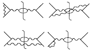
Figure 2: Order $\alpha_{s}$ contributions to the Drell-Yan cross section.

Following Sect. 1.1, we use the factorization formula (11) applied to incoming partons instead of incoming hadrons. Since the details associated with parton masses are going to factorize, we can choose to calculate the cross section for ${\rm parton}\,a+{\rm parton}\,b\to\mu^{+}+\mu^{-}+X$ with the partons having zero mass and transverse momentum. Let us call this cross section $G_{ab}$:

$$\frac{{\rm d}\sigma(a\,b\to\mu^{+}\,\mu^{-}\,X)}{{\rm d}Q^{2}{\rm d}y}=G_{ab}\!\left({x_{A}},{x_{B}},Q;\frac{\mu}{Q};\alpha_{s};\epsilon\right)$$ (18)

In this calculation there are both ultraviolet and infrared divergences. Dimensional regularization is used to regulate them both. The factorization formula is then

$$G_{ab}\!\left({x_{A}},{x_{B}},Q;\frac{\mu}{Q};\alpha_{s};\epsilon\right)=\sum_{c,d}\int_{x_{A}}^{1}{{\rm d}\xi_{A}}\int_{x_{B}}^{1}{{\rm d}\xi_{B}}\ \\ \times f_{c/a}(\xi_{A};\epsilon)\ H_{cd}\!\left(\frac{x_{A}}{\xi_{A}},\frac{x_{B}}{\xi_{B}},Q;\frac{\mu}{Q},\alpha_{s}(\mu);\epsilon\right)\,f_{d/b}(\xi_{B};\epsilon).$$ (19)

Both factors in the formula depend on $\mu$, which is the scale factor introduced in the dimensional regularization and subsequent $\overline{\rm MS}$ renormalization [5] of Green functions of ultraviolet divergent operators. One introduces a factor

$$\left(\frac{\mu^{2}}{4\pi}e^{\gamma}\right)^{\epsilon}$$ (20)

for each integration $\int{\rm d}^{4-2\epsilon}k$ in order to keep the dimensionality of the result independent of $\epsilon$. Ultraviolet divergences then appear as poles in the variable $\epsilon$, which are subtracted away, as explained in [8]. The factor $e^{\gamma}/(4\pi)$ that comes along with the $\mu$ is the difference between $\overline{\rm MS}$ renormalization and minimal subtraction (MS) renormalization. Here $\gamma=0.577\dots$ is Euler’s constant.

Let us suppose that we have calculated $G_{ab}$ to two orders in perturbation theory. We denote the perturbative coefficients by

$$G_{ab}=G_{ab}^{(0)}+\frac{\alpha_{s}}{\pi}\ G_{ab}^{(1)}+{\cal O}(\alpha_{s}^{2}).$$ (21)

Thus $G_{ab}^{(0)}$ is the Born cross section in Eq. (16). $G_{ab}^{(1)}$ is the first correction.

The first correction $G_{ab}^{(1)}$ will generally have ultraviolet divergences at $\epsilon=0$, coming from virtual graphs, and these divergences will appear as $1/\epsilon$ poles. Following the minimal subtraction prescription, we remove these ultraviolet poles as necessary. In general $1/\epsilon$ poles of infrared origin will remain in $G_{ab}^{(1)}$, and we shall discuss these infrared poles presently.

Let us similarly denote the perturbative coefficients of the hard scattering cross section $H_{ab}$ by

$$H_{ab}=H_{ab}^{(0)}+\frac{\alpha_{s}}{\pi}\ H_{ab}^{(1)}+{\cal O}(\alpha_{s}^{2}).$$ (22)

It is these coefficients that we would like to calculate.

All we need to know to calculate $H$ from $G$ is the perturbative expansion of the functions $f_{a/b}(x,\epsilon)$, which, according to the factorization theorem, contain all of the sensitivity to small momenta, and are interpreted as the distribution of parton $a$ in parton $b$. These functions can be calculated in a simple fashion using their definitions (Sect. 4) as matrix elements (here in parton states) of certain operators. When the ultraviolet divergences of the operators are also renormalized using minimal subtraction, one finds simply

$$f_{a/b}(x;\epsilon)=\delta_{ab}\ \delta(1-x)-\frac{1}{2\epsilon}\ \frac{\alpha_{s}}{\pi}\ P_{a/b}^{(1)}(x)+{\cal O}(\alpha_{s}^{2}),$$ (23)

where $P_{a/b}^{(1)}(x)$ is the lowest order Altarelli-Parisi [9] kernel that gives the evolution with $\mu$ of the parton distribution functions. We will discuss the computations that lead to Eq. (23) in Sect. 4. For now, let us assume the result.

When we insert these perturbative expansions (23) into the factorization formula, we obtain

$$\begin{split}G_{ab}^{(0)}\!\left({x_{A}},{x_{B}},Q;\frac{\mu}{Q};\epsilon\right)&+\frac{\alpha_{s}}{\pi}\ G_{ab}^{(1)}\!\left({x_{A}},{x_{B}},Q;\frac{\mu}{Q};\epsilon\right)\\ ={}&H_{ab}^{(0)}\!\left({x_{A}},{x_{B}},Q;\frac{\mu}{Q};\epsilon\right)+\frac{\alpha_{s}}{\pi}\ H_{ab}^{(1)}\!\left({x_{A}},{x_{B}},Q;\frac{\mu}{Q};\epsilon\right)\\ &-\frac{1}{2\epsilon}\ \frac{\alpha_{s}}{\pi}\ \sum_{c}\int_{x_{A}}^{1}{{\rm d}\xi_{A}}\,P_{c/a}^{(1)}(\xi_{A})\ H_{cb}^{(0)}\!\left(\frac{x_{A}}{\xi_{A}},{x_{B}},Q;\frac{\mu}{Q};\epsilon\right)\\ &-\frac{1}{2\epsilon}\ \frac{\alpha_{s}}{\pi}\ \sum_{d}\int_{x_{B}}^{1}{{\rm d}\xi_{B}}\,P_{d/b}^{(1)}(\xi_{B})\ H_{ad}^{(0)}\!\left({x_{A}},\frac{x_{B}}{\xi_{B}},Q;\frac{\mu}{Q};\epsilon\right)\\ &+{\cal O}(\alpha_{s}^{2}).\end{split}$$ (24)

We can now solve for $H_{ab}$. At the Born level, we find

$$H_{ab}^{(0)}\!\left({x_{A}},{x_{B}},Q;\frac{\mu}{Q};\epsilon\right)=G_{ab}^{(0)}\!\left({x_{A}},{x_{B}},Q;\frac{\mu}{Q};\epsilon\right).$$ (25)

Then at the one loop level we obtain

$$\begin{split}H_{ab}^{(1)}\!\left({x_{A}},{x_{B}},Q;\frac{\mu}{Q};\epsilon\right)={}&G_{ab}^{(1)}\!\left({x_{A}},{x_{B}},Q;\frac{\mu}{Q};\epsilon\right)\\ &+\frac{1}{2\epsilon}\ \sum_{c}\int_{x_{A}}^{1}{{\rm d}\xi_{A}}\,P_{c/a}^{(1)}(\xi_{A})\ G_{cb}^{(0)}\!\left(\frac{x_{A}}{\xi_{A}},{x_{B}},Q;\frac{\mu}{Q};\epsilon\right)\\ &+\frac{1}{2\epsilon}\ \sum_{d}\int_{x_{B}}^{1}{{\rm d}\xi_{B}}\,P_{d/b}^{(1)}(\xi_{B})\ G_{ad}^{(0)}\!\left({x_{A}},\frac{x_{B}}{\xi_{B}},Q;\frac{\mu}{Q};\epsilon\right).\end{split}$$ (26)

Thus the prescription is quite simple. One should calculate the cross section at the parton level, $G_{ab}^{(1)}$, and subtract from it certain terms consisting of a divergent factor $1/\epsilon$, the Altarelli-Parisi kernel, and the Born cross section (with $\epsilon\neq 0$). The result is guaranteed to be finite as $\epsilon\to 0$.

Recall that the Born cross section $G^{(0)}$ consists of an $\epsilon$ dependent factor $C(\epsilon)$ times the Born cross section in 4 dimensions, where $C(\epsilon)$ arises from such sources as the integration over the lepton angles in the Drell-Yan process. A convenient way to manage the calculation is to factor $C(\epsilon)$ out of the first order cross section $G^{(1)}$ also. Then the prescription is to remove the $1/\epsilon$ pole in $G^{(1)}(\epsilon)/C(\epsilon)$, set $\epsilon=0$, and multiply by $C(0)=1$. Thus we see that a function of $\epsilon$ that is a common factor to $G_{ab}^{(0)}$ and $G_{ab}^{(1)}$ cancels in the physical hard scattering cross section, as was claimed after Eq. (17).

When calculating $G^{(1)}$, it should be noted that there are contributions involving self energy graphs on the external lines, as in 2. The total of all external line corrections gives a factor of $\sqrt{z_{2}}$ for each external quark (or antiquark) line and $\sqrt{z_{3}}$ for each external gluon line. Here $z_{2}$ and $z_{3}$ are the residues of the poles in the renormalized quark and gluon propagators. In the massless theory these have infrared divergences. For example the value of $z_{2}$ in massless QCD in Feynman gauge is

$$z_{2}=1+\frac{\alpha_{s}}{3\pi\epsilon}+{\cal O}(\alpha_{s}^{2}).$$ (27)

Then the contribution of the self energy graphs to $G^{(1)}$ is a factor $2\alpha_{s}/3\pi\epsilon$ times the Born cross section.

3 Relation to the renormalization group

The prescription (26) for removing infrared poles is intimately related to the $\mu$ dependence of $H_{ab}^{(1)}$ — that is, to the behavior of $H_{ab}^{(1)}$ under the renormalization group. In this section, we display this connection and show how it leads to the approximate invariance of the computed cross section under changes of $\mu$. (Of course, the complete cross section, to all orders of perturbation theory, is exactly invariant under changes of $\mu$. What we are now concerned with is the behavior of a finite-order approximation.)

We recall that the Born cross section $G_{ab}^{(0)}=H_{ab}^{(0)}$ contains some $\mu$ dependence from the factor $C({\mu/Q},\epsilon)$, as specified in Eq. (16). The one loop cross section $G_{ab}^{(1)}$ contains this same factor, and we can simply factor it out of Eq. (26) and set it to 1 when we set $\epsilon=0$ at the end. In addition, $G_{ab}^{(1)}$ contains a factor $\mu^{2\epsilon}$ from the loop integration,

$$\left(\frac{\mu^{2}}{4\pi}e^{\gamma}\right)^{\epsilon}\int{\rm d}^{4-2\epsilon}k.$$ (28)

The $(e^{\gamma}\mu^{2}/4\pi)^{\epsilon}$ factor multiplies the $1/\epsilon$ poles in $G_{ab}^{(1)}$. Writing

$$\frac{A}{\epsilon}\ \mu^{2\epsilon}=\frac{A}{\epsilon}+2A\ \ln(\mu)+{\cal O}(\epsilon),$$ (29)

and reading off the value of $A$ from Eq. (26), we find the $\mu$ dependence of $G_{ab}^{(1)}$ – and thus of $H_{ab}^{(1)}$:

$$\begin{split}H_{ab}^{(1)}\!\left({x_{A}},{x_{B}},Q;\frac{\mu}{Q}\right)=&H_{ab}^{(1)}\!\left({x_{A}},{x_{B}},Q;1\right)\\ &-\ln\!\left(\frac{\mu}{Q}\right)\ \sum_{c}\int_{x_{A}}^{1}{{\rm d}\xi_{A}}\,P_{c/a}^{(1)}(\xi_{A})\ H_{cb}^{(0)}\!\left(\frac{x_{A}}{\xi_{A}},{x_{B}},Q\right)\\ &-\ln\!\left(\frac{\mu}{Q}\right)\ \sum_{d}\int_{x_{B}}^{1}{{\rm d}\xi_{B}}\,P_{d/b}^{(1)}(\xi_{B})\ H_{ad}^{(0)}\!\left({x_{A}},\frac{x_{B}}{\xi_{B}},Q\right).\end{split}$$ (30)

Here we have set $\epsilon=0$ and have suppressed the notation indicating $\epsilon$ dependence; we have also noted that $H^{(0)}$ does not depend on $\mu$ when $\epsilon=0$, so we have suppressed the notation indicating $\mu$ dependence in $H^{(0)}$.

We see that $H^{(1)}$ contains logarithms of $\mu/Q$. If $\mu$ is fixed while $Q$ becomes very large, then these logarithms spoil the usefulness of perturbation theory, since the large logarithms can cancel the small coupling $\alpha_{s}(\mu)$ that multiplies $H^{(1)}$. For this reason, one chooses $\mu$ such that $\ln\!\left(\mu/Q\right)$ is not large. For example, one chooses $\mu=Q$ or perhaps $\mu=2Q$ or $\mu=Q/2$.

The freedom to choose $\mu$ results from the renormalization group equations obeyed by $H$ and $f_{a/A}(\xi)$. The renormalization group equation for $H_{ab}$ is

$$\begin{split}\mu\frac{{\rm d}}{{\rm d}\mu}\ &H_{ab}\!\left({x_{A}},{x_{B}},Q;\frac{\mu}{Q},\alpha_{s}(\mu)\right)\\ =&-\sum_{c}\int_{x_{A}}^{1}{{\rm d}\zeta_{A}}\,P_{c/a}(\zeta_{A},\alpha_{s}(\mu))\ H_{cb}\!\left(\frac{x_{A}}{\zeta_{A}},{x_{B}},Q;\frac{\mu}{Q},\alpha_{s}(\mu)\right)\\ &-\sum_{d}\int_{x_{B}}^{1}{{\rm d}\zeta_{B}}\,P_{d/b}(\zeta_{B},\alpha_{s}(\mu))\ H_{ad}\!\left({x_{A}},\frac{x_{B}}{\zeta_{B}},Q;\frac{\mu}{Q},\alpha_{s}(\mu)\right).\end{split}$$ (31)

Here $P_{c/a}(\xi,\alpha_{s}(\mu))$ is the all orders Altarelli-Parisi kernel. It has a perturbative expansion

$$P_{c/a}(\xi,\alpha_{s}(\mu))=\frac{\alpha_{s}(\mu)}{\pi}\ P_{c/a}^{(1)}(\xi)+\dots$$ (32)

where $P_{c/a}^{(1)}(\xi)$ is the function that appears in Eq. (23). Thus at lowest order the renormalization group equation (31) is a simple consequence of differentiating Eq. (23).

Parton distribution functions also have a $\mu$ dependence, which arises from the renormalization of the ultraviolet divergences in the products of quark and gluon operators in the definitions of these functions, given in Eqs. (43) and (44) below. The renormalization group equation for the distribution functions is

$$\mu\frac{{\rm d}}{{\rm d}\mu}\ f_{a/A}(\xi,\mu) =\sum_{b}\int_{\xi}^{1}\frac{{\rm d}\zeta}{\zeta}\,P_{a/b}\!\left(\zeta,\alpha_{s}(\mu)\right)\ f_{b/A}\!\left(\frac{\xi}{\zeta},\mu\right).$$ (33)

The physical cross section does not, of course, depend on $\mu$, since $\mu$ is not one of the parameters of the Lagrangian, but is rather an artifact of the calculation. Nevertheless, the cross section calculated at a finite order of perturbation theory will acquire some $\mu$ dependence arising from the approximation of throwing away higher order contributions. To see how this comes about, we differentiate Eq. (11) with respect to $\mu$ and use Eqs. (31) and (33). This gives

$$\begin{split}\mu\frac{{\rm d}}{{\rm d}\mu}&~{}\frac{{\rm d}\sigma}{{\rm d}Q^{2}{\rm d}y}=\\ ={}&\sum_{a,b,c}\ \int_{x_{A}}^{1}{{\rm d}\xi_{A}}\,\int_{\xi_{A}}^{1}\frac{{\rm d}\zeta_{A}}{\zeta_{A}}\,\int_{x_{B}}^{1}{{\rm d}\xi_{B}}\\ &\quad P_{a/c}\!\left(\zeta_{A},\alpha_{s}(\mu)\right)\ f_{c/A}\!\left(\frac{\xi_{A}}{\zeta_{A}},\mu\right)H_{ab}\!\left(\frac{x_{A}}{\xi_{A}},\frac{x_{B}}{\xi_{B}},Q;\frac{\mu}{Q},\alpha_{s}(\mu)\right)\,f_{b/B}(\xi_{B},\mu)\\ &-\sum_{a,b,c}\ \int_{x_{A}}^{1}{{\rm d}\bar{\xi}_{A}}\,\int_{x_{A}/\bar{\xi}_{A}}^{1}{{\rm d}\zeta_{A}}\,\int_{x_{B}}^{1}{{\rm d}\xi_{B}}\\ &\quad f_{a/A}\left({\bar{\xi}_{A}},\mu\right)P_{c/a}\!\left(\zeta_{A},\alpha_{s}(\mu)\right)\ H_{cb}\!\left(\frac{x_{A}}{\bar{\xi}_{A}\zeta_{A}},\frac{x_{B}}{\xi_{B}},Q;\frac{\mu}{Q},\alpha_{s}(\mu)\right)\,f_{b/B}(\xi_{B},\mu)\\ &+\mbox{$B$ terms}.\end{split}$$ (34)

Here the two terms shown relate to the evolution of the partons in hadron $A$. As indicated, two similar terms relate to the evolution of the partons in hadron $B$. We now change the order of integration in the second term to put the $\bar{\xi}_{A}$ integration inside the $\zeta_{A}$ integration, then change the integration variable from $\bar{\xi}_{A}$ to $\xi_{A}=\bar{\xi}_{A}\zeta_{A}$, and finally reverse the order of integrations again. This gives

$$\begin{split}\mu\frac{{\rm d}}{{\rm d}\mu}\ &\frac{{\rm d}\sigma}{{\rm d}Q^{2}{\rm d}y}=\\ &\sum_{a,b,c}\ \int_{x_{A}}^{1}{{\rm d}\xi_{A}}\,\int_{\xi_{A}}^{1}\frac{{\rm d}\zeta_{A}}{\zeta_{A}}\,\int_{x_{B}}^{1}{{\rm d}\xi_{B}}\\ &~{}\times P_{a/c}\!\left(\zeta_{A},\alpha_{s}(\mu)\right)\ f_{c/A}\!\!\left(\frac{\xi_{A}}{\zeta_{A}},\mu\right)H_{ab}\!\!\left(\frac{x_{A}}{\xi_{A}},\frac{x_{B}}{\xi_{B}},Q;\frac{\mu}{Q},\alpha_{s}(\mu)\right)\,f_{b/B}(\xi_{B},\mu)\\ &-\sum_{a,b,c}\ \int_{x_{A}}^{1}{{\rm d}\xi_{A}}\,\int_{\xi_{A}}^{1}\frac{{\rm d}\zeta_{A}}{\zeta_{A}}\,\int_{x_{B}}^{1}{{\rm d}\xi_{B}}\\ &~{}\times f_{a/A}\!\!\left({\frac{\xi_{A}}{\zeta_{A}}},\mu\right)P_{c/a}\!\left(\zeta_{A},\alpha_{s}(\mu)\right)\ H_{cb}\!\!\left(\frac{x_{A}}{\xi_{A}},\frac{x_{B}}{\xi_{B}},Q;\frac{\mu}{Q},\alpha_{s}(\mu)\right)\,f_{b/B}(\xi_{B},\mu)\\ &+{B\ \rm terms}.\end{split}$$ (35)

We see that the two terms cancel exactly as long as $P_{a/b}$ and $H_{ab}$ obey the renormalization group equations exactly. Now, when $H_{ab}$ is calculated only to order $\alpha_{s}^{N}$, it only obeys the renormalization group equation (31) to the same order. In this case, we will have

$$\mu\frac{{\rm d}}{{\rm d}\mu}\ \frac{{\rm d}\sigma}{{\rm d}Q^{2}{\rm d}y}={\cal O}(\alpha_{s}^{N+1})\ ,$$ (36)

when the parton distribution functions obey the renormalization group equation with the Altarelli-Parisi kernel calculated to order $\alpha_{s}^{N}$ or better. One thus finds that the result of a Born level calculation can be strongly $\mu$ dependent, but by including the next order the $\mu$ dependence is reduced.

We have argued that one should choose $\mu$ to be on the order of the large momentum scale in the problem, which is $Q$ in the case of the Drell-Yan cross section. We have the right to choose $\mu$ as we wish because the result would be independent of $\mu$ if the calculation were done exactly. The choice $\mu\sim Q$ eliminates the potentially large logarithms in Eq. (30). Another choice is often used. One substitutes for $\mu$ in Eq. (11) the value $\sqrt{\hat{s}}=\sqrt{\xi_{A}\xi_{B}s}$. We now have a value of $\mu$ that depends on the integration variables in the factorization.

Let us examine whether this is valid, assuming that $P_{a/b}$ and $H_{ab}$ are calculated exactly. We replace $\mu$ by

$$\mu(\lambda,\xi_{A},\xi_{B})=\mu_{0}^{1-\lambda}\left(\sqrt{\xi_{A}\xi_{B}s}\right)^{\lambda},\quad\quad 0<\lambda<1.$$ (37)

At $\lambda=0$ we have a valid starting point. When we get to $\lambda=1$ we have the desired ending point. The question is whether the derivative of the cross section with respect to $\lambda$ is zero. Applying the same calculation as before, we obtain instead of Eq. (34) the result

$$\begin{split}\frac{{\rm d}}{{\rm d}\lambda}~{}\frac{{\rm d}\sigma}{{\rm d}Q^{2}{\rm d}y}={}&\sum_{a,b,c}\ \int_{x_{A}}^{1}{{\rm d}\xi_{A}}\,\int_{\xi_{A}}^{1}\frac{{\rm d}\zeta_{A}}{\zeta_{A}}\,\int_{x_{B}}^{1}{{\rm d}\xi_{B}}\,\frac{1}{2}\,\ln\!\left(\frac{\xi_{A}\xi_{B}s}{\mu_{0}^{2}}\right)\\ &\times P_{a/c}\!\left(\zeta_{A},\alpha_{s}(\mu(\lambda,\xi_{A},\xi_{B}))\right)\ f_{c/A}\!\left(\frac{\xi_{A}}{\zeta_{A}},\mu(\lambda,\xi_{A},\xi_{B})\right)\\ &\times H_{ab}\!\left(\frac{x_{A}}{\xi_{A}},\frac{x_{B}}{\xi_{B}},Q;\frac{\mu(\lambda,\xi_{A},\xi_{B})}{Q},\alpha_{s}(\mu)\right)\,f_{b/B}(\xi_{B},\mu(\lambda,\xi_{A},\xi_{B}))\\ &-\sum_{a,b,c}\ \int_{x_{A}}^{1}{{\rm d}\bar{\xi}_{A}}\,\int_{x_{A}/\bar{\xi}_{A}}^{1}{{\rm d}\zeta_{A}}\,\int_{x_{B}}^{1}{{\rm d}\xi_{B}}\ \frac{1}{2}\,\ln\!\left(\frac{\bar{\xi}_{A}\xi_{B}s}{\mu_{0}^{2}}\right)\\ &\times f_{a/A}\left({\bar{\xi}_{A}},\mu(\lambda,\bar{\xi}_{A},\xi_{B})\right)P_{c/a}\!\left(\zeta_{A},\alpha_{s}(\mu(\lambda,\bar{\xi}_{A},\xi_{B}))\right)\\ &\times H_{cb}\!\left(\frac{x_{A}}{\bar{\xi}_{A}\zeta_{A}},\frac{x_{B}}{\xi_{B}},Q;\frac{\mu(\lambda,\bar{\xi}_{A},\xi_{B})}{Q},\alpha_{s}(\mu)\right)\,f_{b/B}(\xi_{B},\mu(\lambda,\bar{\xi}_{A},\xi_{B}))\\ &+B\ {\rm terms}.\end{split}$$ (38)

Now making the same change of variables as before, we obtain

$$\begin{split}\frac{{\rm d}}{{\rm d}\lambda}&~{}\frac{{\rm d}\sigma}{{\rm d}Q^{2}{\rm d}y}={}\\ &\sum_{a,b,c}\ \int_{x_{A}}^{1}{{\rm d}\xi_{A}}\,\int_{\xi_{A}}^{1}\frac{{\rm d}\zeta_{A}}{\zeta_{A}}\,\int_{x_{B}}^{1}{{\rm d}\xi_{B}}\ \frac{1}{2}\,\ln\!\left(\frac{\xi_{A}\xi_{B}s}{\mu_{0}^{2}}\right)\\ &\quad\quad\times P_{a/c}\!\left(\zeta_{A},\alpha_{s}(\mu(\lambda,\xi_{A},\xi_{B}))\right)\ f_{c/A}\!\left(\frac{\xi_{A}}{\zeta_{A}},\mu(\lambda,\xi_{A},\xi_{B})\right)\\ &\quad\quad\times H_{ab}\!\left(\frac{x_{A}}{\xi_{A}},\frac{x_{B}}{\xi_{B}},Q;\frac{\mu(\lambda,\xi_{A},\xi_{B})}{Q},\alpha_{s}(\mu)\right)\,f_{b/B}(\xi_{B},\mu(\lambda,\xi_{A},\xi_{B}))\\ &-\sum_{a,b,c}\ \int_{x_{A}}^{1}{{\rm d}\xi_{A}}\,\int_{\xi_{A}}^{1}\frac{{\rm d}\zeta_{A}}{\zeta_{A}}\,\int_{x_{B}}^{1}{{\rm d}\xi_{B}}\ \frac{1}{2}\,\ln\!\left(\frac{\xi_{A}\xi_{B}s}{\zeta_{A}\mu_{0}^{2}}\right)\\ &\quad\quad\times f_{a/A}\left(\frac{\xi_{A}}{\zeta_{A}},\mu(\lambda,\xi_{A}/\zeta_{A},\xi_{B})\right)P_{c/a}\!\left(\zeta_{A},\alpha_{s}(\mu(\lambda,\xi_{A}/\zeta_{A},\xi_{B}))\right)\\ &\quad\quad\times H_{cb}\!\left(\frac{x_{A}}{\xi_{A}},\frac{x_{B}}{\xi_{B}},Q;\frac{\mu(\lambda,\xi_{A}/\zeta_{A},\xi_{B})}{Q},\alpha_{s}(\mu)\right)\,f_{b/B}(\xi_{B},\mu(\lambda,\xi_{A}/\zeta_{A},\xi_{B}))\\ &+{B\ \rm terms}.\end{split}$$ (39)

We see that the cancellation between the two terms has been spoiled, first by the differences in the values of $\mu(\lambda,\dots)$ in the two terms, but more importantly by the differences in the arguments of the logarithm in the two terms. We conclude that the substitution of $\hat{s}$ for $\mu^{2}$ results in an error of order $\alpha_{s}$ no matter how accurately the hard scattering cross section is calculated. This is not a problem if the hard scattering cross section is calculated only at the Born level, which is, in fact, commonly the case. However, it is wrong to substitute $\hat{s}$ for $\mu^{2}$ when a calculation beyond the Born level is used.

4 The parton distribution functions

The parton distribution functions are indispensable ingredients in the factorization formula (11). We need to know the distribution of partons in a hadron, based on experimental data, in order to obtain predictions from the formula. In addition, we need to know the distribution of partons in a parton in order to calculate the hard scattering cross section $H_{ab}$. The hard scattering cross section is obtained by factoring the parton distribution functions out of the physical cross section. Evidently, the result depends on exactly what it is that one factors out.

4.1 Operator Definitions

In this section, we describe the definition for the parton distribution functions that we use elsewhere in this chapter. A more complete discussion can be found in Ref. [10]. In this definition, the distribution functions are matrix elements in a hadron state of certain operators that act to count the number of quarks or gluons carrying a fraction $\xi$ of the hadron’s momentum. We state the definition in a reference frame in which the hadron carries momentum $P^{\mu}$ with a plus component $P^{+}$, a minus component $P^{-}=m^{2}/2P^{+}$, and transverse components equal to zero. (We use $P^{\pm}=(P^{0}\pm P^{3})/\sqrt{2}$).

The definition may be motivated by looking at the theory quantized on the plane $x^{+}=0$ in the light-cone gauge $A^{+}=0$, since it is in this picture that field theory has its closest connection with the parton model [11]. In this gauge, ${\cal G}=1$, where ${\cal G}$ is a path-ordered exponential of the gluon field that appears in the definition of the parton distributions. The light-cone gauge tends to be rather pathological if one goes beyond low order perturbation theory, and covariant gauges are preferred for a complete treatment. However quantization on a null plane in the light-cone gauge provides a useful motivation for the complete treatment.

In this approach the quark field has two components that represent the independent degrees of freedom; $\gamma^{+}\psi(x)$ contains these components and not the other two. One can expand the two independent components in terms of quark destruction operators $b(k^{+},{k_{\perp}},s)$ and antiquark creation operators $d(k^{+},{k_{\perp}},s)^{\dagger}$ as follows:

$$\gamma^{+}\psi(0,x^{-},{{x_{\perp}}})=\frac{1}{(2\pi)^{3}}\sum_{s}\int_{0}^{\infty}\frac{{\rm d}k^{+}}{2k^{+}}\int{\rm d}{k_{\perp}}\\ \times\left[\gamma^{+}U(k,s)e^{-ik\cdot x}b(k^{+},{k_{\perp}},s)+\gamma^{+}V(k,s)e^{+ik\cdot x}d(k^{+},{k_{\perp}},s)^{\dagger}\right].$$ (40)

The quark distribution function is just the hadron matrix element of the operator that counts the number of quarks.

$$f_{q/A}(\xi)\,{\rm d}\xi=\frac{1}{(2\pi)^{3}}\sum_{s}\frac{{\rm d}(\xi P^{+})}{2(\xi P^{+})}\int{\rm d}{k_{\perp}}\ \langle P|\,b(\xi P^{+},{k_{\perp}},s)^{\dagger}b(\xi P^{+},{k_{\perp}},s)\,|P\rangle.$$ (41)

In terms of $\psi(x)$, this is

$$f_{q/A}(\xi)=\frac{1}{4\pi}\int{\rm d}x^{-}e^{-i\xi P^{+}x^{-}}\langle P|\bar{\psi}(0,x^{-},{0_{\perp}})\,\gamma^{+}\,\psi(0,0,{0_{\perp}})|P\rangle.$$

We can keep this same definition, while allowing the possibility of computing in another gauge, by inserting the operator

$${\cal G}=\mathcal{P}\,\exp\left\{ig\int_{0}^{x^{-}}{\rm d}y^{-}A_{c}^{+}(0,y^{-},{0_{\perp}})t_{c}\right\},$$ (42)

where $\mathcal{P}$ denotes an instruction to order the gluon field operators $A_{a}^{+}(0,y^{-},{0_{\perp}})$ along the path. The operator ${\cal G}$ is evidently 1 in the $A^{+}=0$ gauge. With this operator, the definition is gauge invariant.

We thus arrive at the definition [10, 12]

$$f_{q/A}(\xi)=\frac{1}{4\pi}\int{\rm d}x^{-}e^{-i\xi P^{+}x^{-}}\langle P|\bar{\psi}(0,x^{-},{0_{\perp}})\,\gamma^{+}\,{\cal G}\,\psi(0,0,{0_{\perp}})|P\rangle.$$ (43)

For gluons, the definition based on the same physical motivation is

$$f_{g/A}(\xi)=\frac{1}{2\pi\xi P^{+}}\int{\rm d}x^{-}e^{-i\xi P^{+}x^{-}}\langle P|F_{a}(0,x^{-},{0_{\perp}})^{+\nu}\,{\cal G}_{ab}\,F_{b}(0,0,{0_{\perp}})_{\nu}^{\ +}\,|P\rangle,$$ (44)

where $F_{\mu\nu}^{a}$ is the gluon field strength operator and where in ${\cal G}$ we now use the octet representation of the SU(3) generating matrices $t_{c}$.

4.2 Feynman rules and eikonal lines

The Feynman rules for parton distributions are derived in a straightforward manner from the standard Feynman rules. Consider, for instance the distribution $f_{q/q}$ of a quark in a quark. To compute this quantity in perturbation theory, we use the following identity satisfied by any ordered exponential,

$$\mathcal{P}\ \exp\Bigl{\{}ig\int_{0}^{\eta}{\rm d}\lambda\,n\cdot A(\lambda n^{\mu})\Bigr{\}}=\\ \Bigl{[}\mathcal{P}\ \exp\Bigl{\{}ig\int_{0}^{\infty}{\rm d}\lambda\,n\cdot A((\lambda+\eta)n^{\mu})\Bigr{\}}\Bigr{]}^{\dagger}\ P\ \exp\Bigl{\{}ig\int_{0}^{\infty}{\rm d}\lambda\,n\cdot A(\lambda n^{\mu})\Bigr{\}}\ .$$ (45)

Using (45) in Eq. (43), for instance, enables us to insert a complete set of states and write

$$f_{q/q}(\xi)=\frac{1}{4\pi}\int{\rm d}x^{-}e^{-\xi P^{+}x^{-}}\sum_{n}\langle P|{\bar{\Psi}}(0,x^{-},{0_{\perp}})|n\rangle\,\gamma^{+}\,\langle n|\Psi(0,0,{0_{\perp}})|P\rangle\ ,$$ (46)

where we define $\Psi$ as the quark field times an associated ordered exponential,

$$\Psi(x)\equiv\psi(x)\ \mathcal{P}\,\exp\left[ig\int_{0}^{\infty}{\rm d}\lambda\,v\cdot A(x+\lambda v^{\mu})\right]\ ,$$ (47)

where $v^{\mu}\equiv g^{\mu}_{-}$, and $A^{\mu}(x)\equiv A^{\mu}_{c}(x)t_{c}$. To express the matrix elements in Eq. (46) in terms of diagrams, we note that by (47) the gluon fields in the expansion of $\Psi$ are time ordered by construction. Expanding the ordered exponentials, and expressing them in momentum space we find

$$\mathcal{P}\ \exp\left[ig\int_{0}^{\infty}{\rm d}\lambda\,n\cdot A(\lambda n^{\mu})\right]=\\ 1+\mathcal{P}\sum_{n=1}^{\infty}\prod_{i=1}^{n}\int\frac{{\rm d}^{4}q_{i}}{(2\pi)^{4}}\,g\,n\cdot{\tilde{A}}(q_{i}^{\mu})\frac{1}{n\cdot\sum_{j=1}^{i}q_{j}+i\epsilon}\ ,$$ (48)

where we define the operator P on the right-hand side of the equation to order the fields with the lowest value of $i$ to the left. From Eq. (48) we can read off the Feynman rules for the expansion of the ordered exponential [10, 12]. They are illustrated in Fig. 3.

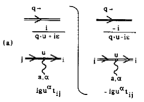
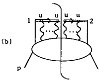
Figure 3: (a) Feynman rules for eikonal lines in the amplitude and its complex conjugate. (b) A general contribution to a parton distribution.

The denominators $n\cdot\sum_{j}q_{j}+i\epsilon$ are represented by double lines, which we shall refer to as “eikonal” lines. These lines attach to gluon propagators via a vertex proportional to $-ign^{\mu}$. Fig. 3(a) shows the formal Feynman rules for eikonal lines and vertices. In Fig. 3(b), we show a general contribution to $f_{q/q}$, as defined by Eq. (46).

The positions of all the explicit fields in Eq. (46) differ only in their plus components. As a result, minus and transverse momenta are integrated over. (They may thought of as flowing freely through the eikonal line.) The plus momentum flowing out of vertex $1$ and into vertex $2$, however, is fixed to be $\xi P^{+}$. No plus momentum flows across the cut eikonal line in the figure. Fig. 4 shows the one loop corrections to $f_{q/q}(\xi)$.

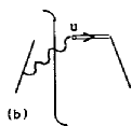
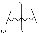
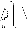
Figure 4: One loop corrections to quark distribution, Eq. (43).

To be explicit, Fig. 4(b) is given in $n$ dimensions by

$$\frac{1}{4\pi}\frac{4}{3}\int\frac{{\rm d}^{n}q}{(2\pi)^{n}}\,N_{\alpha\beta}(q)\,2\pi\delta(q^{2})\,\frac{i}{(p-q)^{2}+i\epsilon}\ \times\\ \times\mathop{\rm tr}[(\hbox to0.0pt{/\hss}p-\hbox to0.0pt{/\hss}q)(-ig\gamma^{\alpha})\hbox to0.0pt{/\hss}p\gamma^{+})]\,(ig\mu^{\epsilon}n^{\beta})\ \frac{-i}{u\cdot q-i\epsilon},$$ (49)

where $N_{\alpha\beta}$ is the polarization tensor of the gluon. By applying minimal subtraction to Eq. (49) and the similar forms for the other diagrams in Fig. 4, we easily verify Eq. (23) for $f_{q/q}$. Gluon distributions are calculated perturbatively in a similar manner. We will need the concept of eikonal lines again, when we discuss the proof of factorization in gauge theories.

4.3 Renormalization

The operator products in the definitions (43) and (44) require renormalization, as discussed in Ref. [10]. We choose to renormalize using the $\overline{\rm MS}$ scheme. Of course, renormalization introduces a dependence on the renormalization scale $\mu$. The renormalization group equation for the $f_{a/A}$ is the Altarelli-Parisi equation (33). A complete derivation of this result may be found in Ref. [10].

The one-loop result, Eq. (23), can actually be understood without looking at the details of the calculation. At order $\alpha_{s}$, one has simple one loop diagrams that contain an ultraviolet divergence that arises from the operator product, but also contain an infrared divergence that arises because we have massless, on-shell partons as incoming particles. The transverse momentum integral is zero, due to a cancellation of infrared and ultraviolet poles, which we may exhibit separately:

$$\left(\frac{\mu^{2}}{4\pi}e^{\gamma}\right)^{\epsilon}\int\frac{{\rm d}^{2-2\epsilon}{k_{\perp}}}{(2\pi)^{2-2\epsilon}}\ \frac{1}{{k_{\perp}}^{2}}=\frac{1}{4\pi}\left\{\frac{1}{\epsilon_{\rm\scriptscriptstyle UV}}-\frac{1}{\epsilon_{\rm\scriptscriptstyle IR}}\right\}.$$ (50)

In this way, we obtain

$$f_{a/b}(\xi;\epsilon)=\delta_{ab}\ \delta(1-\xi)+\left\{\frac{1}{\epsilon_{\rm\scriptscriptstyle UV}}-\frac{1}{\epsilon_{\rm\scriptscriptstyle IR}}\right\}\frac{\alpha_{s}}{\pi}\ P_{a/b}^{(1)}(\xi)-{\rm counterterm}+{\cal O}(\alpha_{s}^{2}).$$ (51)

The coefficient of $1/\epsilon_{\rm\scriptscriptstyle UV}$ is the ‘anomalous dimension’ that appears in the renormalization group equation, that is, the Altarelli-Parisi kernel. Following the $\overline{\rm MS}$ renormalization scheme, we use the counter term to cancel $1/\epsilon_{\rm\scriptscriptstyle UV}$ term. This leaves the infrared $1/\epsilon$, which is not removed by renormalization,

$$f_{a/b}(\xi;\epsilon)=\delta_{ab}\ \delta(1-\xi)-\frac{1}{\epsilon}\frac{\alpha_{s}}{\pi}\ P_{a/b}^{(1)}(\xi)+{\cal O}(\alpha_{s}^{2}).$$ (52)

4.4 Relation to Structure Functions

Let us now consider the relation of the parton distribution functions to the structure functions measured in deeply inelastic lepton scattering. If we use the definition of parton distribution functions given above, then the structure function $F_{2}$ is given by the factorization equation (2). At the Born level, the hard scattering function is simply zero for gluons and the quark charge squared, $e_{j}^{2}$, times a delta function for quarks. Thus the formula for $F_{2}$ takes the form

$$\begin{split}x^{-1}F_{2}(x,Q)={}&\sum_{j}e_{j}^{2}\ f_{j/A}(x,\mu)+\sum_{j,b}e_{j}^{2}\int_{x}^{1}\frac{{\rm d}\xi}{\xi}\ f_{b/A}(\xi,\mu)\,\frac{\alpha_{s}}{\pi}\,C_{jb}\left(\frac{x}{\xi},\frac{Q}{\mu}\right)\\ &+{\cal O}(\alpha_{s}^{2}).\end{split}$$ (53)

The sums over $j$ run over all flavors of quarks and antiquarks. Gluons do not contribute at the Born level, but they do at order $\alpha_{s}$, through virtual quark-antiquark pairs. The hard scattering coefficients $C_{jb}$ can be obtained by calculating (at order $\alpha_{s}$) deeply inelastic scattering from on-shell massless partons, then removing the infrared divergences according to the scheme discussed in Sect. 2.

The explicit form of the perturbative coefficients $C_{jb}$ is [5]

$$C_{jk}(z,1)={} \delta_{jk}\,\frac{4}{3}\left[-\frac{1}{2}\frac{1+z^{2}}{1-z}\,\ln\!\left(\frac{z}{1-z}\right)+\frac{3}{4}\frac{1}{1-z}-\frac{3}{2}-z\right]_{+}$$

$$C_{jg}(z,1)={} -\frac{1}{2}\left\{\frac{1}{2}\left[z^{2}+(1-z)^{2}\right]\,\left[\ln\!\left(\frac{z}{1-z}\right)+1\right]\,-3z(1-z)\right\},$$ (54)

where the plus subscript to the bracket in the first equation denotes a subtraction that regulates the $z\to 1$ singularity,

$$\int_{x}^{1}{\rm d}z\ [C(z)]_{+}\ h(z) = \int_{0}^{1}{\rm d}z\ [C(z)]_{+}\ h(z)\,\Theta(z>x)$$ (55)

$$= \int_{0}^{1}{\rm d}z\ C(z)\ \Bigl{\{}h(z)\,\Theta(z>x)-h(1)\Bigr{\}}.$$

4.5 Other Parton Distributions

The definitions (43) and (44) are the most natural for many purposes. They are not, however, unique. Indeed, any function $g_{b/A}(y)$, which can be related to $f_{a/A}(x)$ by convolution with ultraviolet functions $D_{ab}(x/y,Q/\mu)$ in a form like

$$g_{a/A}(x)=\sum_{b}\int_{x}^{1}({\rm d}y/y)\,D_{ab}(x/y,Q/\mu,\alpha_{s}(\mu))\,f_{b/A}(y)\ ,$$ (56)

is an acceptable parton distribution [13]. The hard scattering functions calculated with the distributions $g_{b/A}$ will differ from those calculated with $f_{a/A}(x)$, but this difference will itself be calculable from the functions $D_{ab}$ as a power series in $\alpha_{s}(Q)$.

The most widely used parton distribution of this type is based on deeply inelastic scattering, and may be called the DIS definition. The definition is

$$f_{j/A}^{\rm DIS}(x,\mu)=f_{j/A}(x,\mu)+\sum_{b}\int_{x}^{1}\frac{{\rm d}\xi}{\xi}f_{b/A}(\xi,\mu)\,\frac{\alpha_{s}}{\pi}\,C_{jb}\left(\frac{x}{\xi},1\right)+{\cal O}(\alpha_{s}^{2}).$$ (57)

for quarks or antiquarks of flavor $j$. Comparing this definition with Eq. (53), we see that

$$x^{-1}F_{2}(x,Q)=\sum_{j}e_{j}^{2}\ f_{j/A}^{\rm DIS}(x,Q)+{\cal O}(\alpha_{s}^{2}).$$ (58)

That is, we adjust the definition so that the order $\alpha_{s}$ correction to deeply inelastic scattering vanishes when $\mu=Q$. It is not so clear what one should do with the gluon distribution in the DIS scheme. One choice [14] is

$$f_{g/A}^{\rm DIS}(x,\mu)=f_{g/A}(x,\mu)-\sum_{j}\sum_{b}\int_{x}^{1}\frac{{\rm d}\xi}{\xi}f_{b/A}(\xi,\mu)\frac{\alpha_{s}}{\pi}C_{jb}\left(\frac{x}{\xi},1\right)+{\cal O}(\alpha_{s}^{2}).$$ (59)

This has the virtue that it preserves the momentum sum rule that is obeyed by the $\overline{\rm MS}$ parton distributions [10],

$$\sum_{a}\int_{0}^{1}{\rm d}\xi\ f_{a/A}(x,\mu)=1.$$ (60)

If one wishes to use parton distribution functions with the DIS definition, then one must modify the hard scattering function for the process under consideration. One should combine Eqs. (52) and (59) to get the DIS distributions of a parton in a parton, then use these distributions in the derivation in Sect. 2.

It should be noted that there is some confusion in the literature concerning the term $+1$ that follows the logarithm in $C_{jg}$ in Eq. (54). The form quoted is the original result of Ref. [5], translated from moment-space to $z$-space. In the calculation with incoming gluons, one normally averages over polarizations of the incoming gluons instead of using a fixed polarization. This means that one sums over polarizations and divides by the number of spin states of a gluon in $4-2\epsilon$ dimensions, namely $2-2\epsilon$. If, instead, one divides by 2 only, one obtains the result (54) without the $+1$, which may be found in Ref. [15]. This does no harm if, as in the case of Ref. [15], one wants to express the cross section for a second hard process in terms of DIS parton distribution functions and if one consistently divides by 2 instead of $2-2\epsilon$ in both processes. However, it is not correct if one wants to relate the DIS structure functions to $\overline{\rm MS}$ parton distribution functions, defined as hadron matrix elements of the appropriate operators, renormalized by $\overline{\rm MS}$ subtraction.

5 Factorization for $\phi^{3}$ Theory

In this and the next section, we study the factorization theorem in a $\phi^{3}$ theory for $n\leq 6$ space-time dimensions. First we show how the factorization theorem comes about for one-loop corrections in deeply inelastic scattering, and compare the field theory to the parton model. In the next section, we will present a reasonably complete but compact derivation of the factorization theorem in deeply inelastic scattering to all orders of perturbation theory.

The scalar theory allows us to study these issues in a simplified but highly nontrivial context. As emphasized above, the purpose of the factorization theorems is to separate long-distance behavior in perturbation theory. In the scalar theory, as we shall see, this behavior is associated with partons that are collinear to the observed hadrons. The organization of such “collinear divergences” is central to factorization in all field theories, but in gauge theories they are joined by “soft” partons, associated with infrared divergences. Indeed, the basic problem in gauge theories is to show how that infrared or “soft” divergences cancel (see Sect. 9). In $\phi^{3}$ theory the infrared problem is absent, so that studying this theory allows us to study the basic physics of factorization in the simplest possible setting.

The Lagrangian is

$${\cal L}=\frac{1}{2}\left(\partial\phi\right)^{2}-\frac{1}{2}m^{2}\phi^{2}-\frac{1}{6}g(\mu^{2}e^{\gamma}/4\pi)^{\epsilon/2}\phi^{3}+\mbox{counterterms}\ .$$ (61)

We will use, where necessary, dimensional regularization, with space-time dimension $n=6-2\epsilon$. It is worth recalling that at $n=6$ the theory is renormalizable, while for $n<6$ it is superrenormalizable. We shall not concern ourselves with the theory for $n>6$ where it is nonrenormalizable by power-counting. $\mu$ is a mass which enables us to keep $g$ dimensionless as we vary $n$. We will renormalize the theory with the $\overline{\rm MS}$ prescription. We use the factor $(\mu^{2}e^{\gamma}/4\pi)^{\epsilon/2}$ rather than the more conventional $\mu^{\epsilon}$, so that we can implement $\overline{\rm MS}$ renormalization as pure pole counterterms. (For convenience, we will define the $h\phi$ counterterm that renormalizes the tadpole graphs by requiring the sum of the tadpoles and their counterterm to vanish.) We define

$$\bar{\mu}=\mu\sqrt{e^{\gamma}/4\pi}.$$ (62)

5.1 Deeply inelastic scattering

Our model for deeply inelastic scattering consists of the exchange of a weakly interacting boson, $A$, not included in the Lagrangian (61). This is illustrated diagrammatically in the same way as for QCD, in Fig. 5. The weak boson couples to the $\phi$ field through an interaction proportional to $\frac{1}{2}A\phi^{2}$. There is then a single structure function which we define by

$$F(x,Q)=\frac{Q^{2}}{2\pi}\int{\rm d}^{6}y\,e^{iq\cdot y}\langle p|j(y)\,j(0)|p\rangle,$$ (63)

where $j=\frac{1}{2}\phi^{2}$. The momentum transfer is $q^{\mu}$, and the usual scalar variables are defined by $Q^{2}=-q^{2}$ and $x=Q^{2}/2p\cdot q$, with $p^{\mu}$ the momentum of the target. We will investigate the structure function in the Bjorken limit of large $Q$ with $x$ fixed, and our calculations will be for the case that the state $|p\rangle$ is a single $\phi$ particle (with non-zero mass, as given in Eq. (61)).

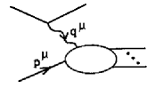
Figure 5: Deeply inelastic scattering.

When $Q$ is large, each graph for the structure function behaves like a polynomial of $\ln(Q/m)$ plus corrections that are nonleading by a power of $Q$. Factorization is possible because only a limited set of momentum regions of the space of loop and final state phase space momenta contribute to the leading power. First we will explain the power counting arguments that determine these “leading regions”, and how they are related to the physical arguments of the parton model.

The tree graph for the structure function is easy to calculate. It is

$$F_{0}=Q^{2}\delta(2p\cdot q+q^{2})=\delta(x-1).$$ (64)

The one-loop “cut diagrams” (as defined in Sect. 2 above) which contribute to $F$ are given in Fig. 6.

Figure 6: One-loop corrections to deeply inelastic scattering. For graphs (b), (d) and (e), we also have the hermitian conjugate graphs.

Each of these diagrams illustrates a different bit of the physics, so we shall treat them in turn, starting with the “ladder” correction, Fig. 6(a).

5.2 Ladder Graph and its Leading Regions

The Feynman integral for the cut diagram Fig. 6(a) is

$$F_{2(a)}=\frac{g^{2}Q^{2}{\bar{\mu}}^{2\epsilon}}{(2\pi)^{5-2\epsilon}}\int{\rm d}^{6-2\epsilon}k\frac{\delta((p-k)^{2}-m^{2})\,\delta((q+k)^{2}-m^{2})}{(m^{2}-k^{2})^{2}}.$$ (65)

Although for nonzero $m$ this integral is finite, it will prove convenient to retain the dimensional regularization, in order to display some very important dimension-dependent features of the $Q\to\infty$ limit.

Equation (65) is calculated conveniently in terms of light-cone coordinates. Without loss of generality, we may choose the external momenta, $q^{\mu}$ and $p^{\mu}$ to be $p^{\mu}=(p^{+},m^{2}/2p^{+},{0_{\perp}})$ and $q^{\mu}=(-xp^{+},Q^{2}/2xp^{+},{0_{\perp}})$. Notice that this formula for $q^{\mu}$ corresponds to a slight change in the definition of $x$, which we now define by $Q^{2}/2p\cdot q\equiv x/(1-xm^{2}/Q^{2})$. At leading power in $Q$, there is no difference, but at finite energy our formulas will be simplified by this choice.

The $\delta$-functions in (65) can be used to perform the ${k_{\perp}}$ and $k^{-}$ integrals. Then if we set $\xi=k^{+}/p^{+}$, we find

$$F_{2(a)} = \frac{g^{2}}{64\pi^{3}}\left(\frac{Q^{2}}{e^{\gamma}\mu^{2}x(1-x)}\right)^{-\epsilon}\frac{1}{\Gamma(2-\epsilon)}\,\left(1-\frac{m^{2}x}{Q^{2}}\right)^{1-\epsilon}$$ (66)

$$\times\int_{\xi_{\rm min}}^{\xi_{\rm max}}{\rm d}\xi\,\frac{x[(\xi_{\rm max}-\xi)(\xi-\xi_{\rm min})]^{1-\epsilon}}{[\xi-x-x^{2}(1-\xi)m^{2}/Q^{2}]^{2}}\ ,$$

where the limits $\xi_{\rm min}$ and $\xi_{\rm max}$ are given by

$$\frac{1+x}{2}\pm\frac{1-x}{2}\sqrt{1-\frac{4m^{2}x}{(1-x)(Q^{2}+m^{2}x)}}\ .$$ (67)

In this form, we can look for the leading regions of the ladder corrections. To do this, it is simplest to set the mass to zero, find the leading regions, and then check back as to whether we must reincorporate the mass in the actual calculation. So, to lowest order in $\Delta\equiv m^{2}/Q^{2}$, (66) becomes

$$F_{2(a)} = \frac{g^{2}}{64\pi^{3}}\left(\frac{Q^{2}}{e^{\gamma}\mu^{2}x(1-x)}\right)^{-\epsilon}\!\frac{1}{\Gamma(2-\epsilon)}$$ (68)

$$\times\int_{x(1+\Delta)}^{1}\!{\rm d}\xi\,\frac{x\left\{(1-\xi)[\xi-x(1+\Delta)]\right\}^{1-\epsilon}}{\left\{\xi-x[1+x(1-\xi)\Delta]\right\}^{2}}.$$

To interpret this expression, we must distinguish between the renormalizable ($n=6,\epsilon=0)$ and superrenormalizable $(n<6,\epsilon>0)$ cases.

In the super-renormalizable case, ($\epsilon>0$), the leading-power contribution $(Q/\mu)^{0}$ comes from near the endpoint $\xi=x(1+\Delta)$. The bulk of the integration region, where $\xi-x=O(1)$ is suppressed by a power of $Q$. The integral is power divergent when $m=0$, and clearly we cannot neglect the mass.

Now consider the renormalizable case, $n=6$. When we set $\epsilon=0$, Eq. (68) has leading power ($Q^{0}$) contributions from both the region $\xi-x$ near zero, where, as above, the mass may not be neglected, and the region $\xi-x=O(1)$, where it may. In the former region, the integral is logarithmically divergent for zero mass, but since the nonzero mass acts as a cutoff, the two regions $\xi\sim x$ and $\xi-x=O(1)$ should be thought of as giving contributions of essentially equal importance. We now interpret these dimension-dependent leading regions.

5.3 Collinear and Ultraviolet Leading Regions; the Parton Model

To see the physical content of the leading regions identified above, it is useful to relate the variable $\xi$ in (66) to the momentum $k^{\mu}$, by the relations

$$k^{+} = \xi p^{+},$$

$$k^{-} = \frac{-1}{2p^{+}(1-x)}\left[\left(\frac{\xi}{x}-1\right)Q^{2}-m^{2}(1-\xi)\right],$$

$${k_{\perp}}^{2} = \frac{Q^{2}(1-\xi)(\xi-x)}{x(1-x)}-\frac{m^{2}[(1-\xi)^{2}+\xi(1-x)]}{1-x}.$$ (69)

Changing variables to ${k_{\perp}}^{2}$, we now rewrite the integral Eq. (68) in a form which is accurate to leading power in $\Delta$ for $n<6$,

$$F_{2(a)}=\frac{g^{2}}{64\pi^{3}}\frac{1}{\Gamma(2-\epsilon)}\int_{0}{\rm d}{k_{\perp}}^{2}\,\frac{[{k_{\perp}}^{2}]^{1-\epsilon}\,(\mu^{2}e^{\gamma})^{\epsilon}}{({k_{\perp}}^{2}+m^{2}(1-x+x^{2}))^{2}}\ .$$ (70)

We emphasize that this expression is accurate to leading power in the region ${k_{\perp}}^{2}/Q^{2}=O(\Delta)$, which is sufficient to give the full leading power for $n<6$, although not for $n=6$, where larger ${k_{\perp}}$ also contribute.

Now let us choose a frame in which $p^{+}$ is of order $Q$. When $\xi\to x$, the components of $k^{\mu}$ are of order $(Q,(\xi-x)Q,Q\sqrt{\xi-x})$, and at its lower limit, $\xi-x$ is of order $m^{2}/Q^{2}$. Hence, in the region that gives the sensitivity to $m$, ${k_{\perp}}$ is small, and $k^{\mu}$ is ultrarelativistic and represents a particle moving nearly collinear to the incoming momentum, $p^{\mu}$. In addition, the on-shell line, of momentum $p^{\mu}-k^{\mu}$, is nearly collinear to the incoming line as well. In fact, when $m$ and ${k_{\perp}}$ are both zero, $k^{\mu}$ is also on the mass shell. The energy deficit necessary to put both the momenta $k^{\mu}$ and $p^{\mu}-k^{\mu}$ on shell is of order ${k_{\perp}}^{2}/Q$ in this frame. Thus, in this frame, the intermediate state represented by the Feynman diagram lives a time of order $Q/{k_{\perp}}^{2}$, which diverges in the collinear limit. The space-time picture for such a process is illustrated in Fig. 7, and we see a close relation to the parton model, as discussed in Sect. 1.4, which depends on the time dilation of partonic states. Partonic states whose energy deficit is much greater than $m$ in the chosen frame correspond to $\xi-x$ of order unity, and do not contribute at leading twist. Thus here, as in the parton model, there is a clear separation between long-lived, time-dilated states which contribute to the distribution of partons from which the scattering occurs, and the hard scattering itself, which occurs on a short time scale.

Figure 7: Space-time structure of collinear interaction.

From this discussion, the collinear region, which is the only leading region when $n$ is less than 6, is naturally described in parton model language.

When $n=6$, the collinear region remains leading. In addition, however, all scales between ${k_{\perp}}=m$ and ${k_{\perp}}=Q$ contribute at leading power, and there is no natural gap between long- and short-distance interactions. When $\xi-x$ is order unity, $k^{\mu}$ is separated from $p^{\mu}$ by a finite angle, and corresponds to a short-lived intermediate state, where $(p-k)^{2}\gg m^{2}$. This leading region, which is best described as “ultraviolet”, is not naturally described by the parton model. But, in an asymptotically free theory (as ${(\phi^{3})}_{6}$ is), such short-lived states may still be treated perturbatively. We shall see how to do this below.

In summary, the ladder diagram shows two important features: a strong correspondence with the parton model from leading collinear regions for both superrenormalizable and renormalizable theories and, for the renormalizable theory only, leading ultraviolet contributions, not present in the parton model.

5.4 Parton distribution functions and parton model

We shall now freely generalize the results for the one loop ladder diagram. Indeed, as we shall see in Sect. 7, some of the dominant contributions to the structure function arise from (two-particle-reducible) graphs of the form of Fig. 8. A single parton of momentum $k^{\mu}$ comes out of the hadron and undergoes a collision in the Born approximation. If we temporarily neglect all other contributions, we find that

$$F(x,Q)=\int\frac{{\rm d}^{6}k}{(2\pi)^{6}}\Phi(k,p)H(k,q)+{\cal O}(1/Q^{a}),$$ (71)

where $\Phi$ represents the hadronic factor in the diagram and $H$ the hard scattering (multiplied by the factor of $Q^{2}/2\pi$ in the definition of the structure function):

$$H(k,q)=Q^{2}\delta((k+Q)^{2}-m^{2}).$$ (72)

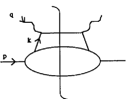
Figure 8: Dominant graphs for deeply inelastic scattering in parton model.

For $\phi^{3}$ with $n<6$, as in the parton model, the parton momentum $k^{\mu}$ is nearly collinear to the hadron momentum $p^{\mu}$. This implies that we can neglect $m$ and the minus and transverse components of $k^{\mu}$ in the hard scattering, so that we can write

$$H=H(x/\xi,Q)=\delta(\xi/x-1),$$ (73)

and hence

$$F(x,Q)=\int_{0}^{1}{\rm d}\xi\left[\int p^{+}\frac{{\rm d}k^{-}{\rm d}^{4}{k_{\perp}}}{(2\pi)^{6}}\Phi(k,p)\right]\delta(\xi/x-1)+{\cal O}(1/Q^{a}).$$ (74)

Here we define $\xi=k^{+}/p^{+}$. The limits on the $\xi$ integral are 0 to 1, since the final state must have positive energy. We therefore define the parton distribution function (or number density):

$$f(\xi) = \xi p^{+}\int\frac{{\rm d}k^{-}{\rm d}^{4}{k_{\perp}}}{(2\pi)^{6}}\,\Phi(k,p)$$ (75)

$$= \int\frac{{\rm d}^{6}k}{(2\pi)^{6}}\,\Phi(k,p)\,\delta(\xi p^{+}/k^{+}-1).$$

With this definition (74) becomes

$$F(x,Q) = \int\frac{{\rm d}\xi}{\xi}\,f(\xi)\,H(x/\xi,Q)+{\cal O}(1/Q^{a})$$ (76)

$$= f(x)+{\cal O}(1/Q^{a})\qquad(n<6).$$

As we shall see in the next section, the factorization theorem is also true in the renormalizable theory,

$$F(x,Q)=\int\frac{{\rm d}\xi}{\xi}\,f(\xi)\,H(x/\xi,Q)+{\cal O}(1/Q^{a})\qquad(n=6)\ ,$$ (77)

where now $H$ is nontrivial. The dominant processes that contribute are illustrated by Fig. 9, which generalizes the parton model only to the extent of having more than just the Born graph for the hard scattering. These processes first involve interactions within the hadron that take place over a long time scale before the interaction with the virtual photon. Then one parton out of the hadron interacts over a relatively short time scale.

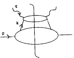
Figure 9: Dominant regions for deeply inelastic scattering in ${(\phi^{3})}_{6}$ theory.

We now note that Eq. (75) can be expressed in operator form as

$$f(\xi)=\frac{\xi p^{+}}{2\pi}\int_{-\infty}^{\infty}{\rm d}y^{-}e^{-i\xi p^{+}y^{-}}\langle p|\,\phi(0,y^{-},{0_{\perp}})\,\phi(0)\,|p\rangle.$$ (78)

This is the definition which we use for all $n\leq 6$. Of course in the renormalizable theory $n=6$ renormalization will be necessary [10]. The definition (78) is precisely the analog for $\phi^{3}$ theory of those we gave in Sect. 4 for QCD. It involves an integral over a bilocal operator along a light-like direction. The graphs for $f(\xi)$ up to one-loop order are shown in Fig. 10. Feynman rules are the same as for the gauge theory, but without eikonal lines.

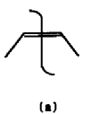
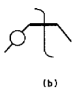
Figure 10: Low-order graphs for parton distribution in $\phi^{3}$ theory.

It is natural to interpret $f(x){\rm d}x$ as the number of partons with fractional momenta between $x$ and $x+{\rm d}x$. This interpretation is justified by the use of light front quantization [11], as we saw in Sect. 4. Note that although the definition picks out a particular direction as special to the problem, it is invariant under boosts parallel to this direction.

The ladder graph, Fig. 10(c) gives

$$f_{c}=\frac{g^{2}{\bar{\mu}}^{2\epsilon}}{(2\pi)^{6-2\epsilon}}\int{\rm d}^{6-2\epsilon}k\,\delta(\xi p^{+}/k^{+}-1)\,\frac{2\pi\,\delta\left((p-k)^{2}-m^{2})\right)}{(m^{2}-k^{2})^{2}}.$$ (79)

The $\delta$-functions may be used to perform the $k^{+}$ and $k^{-}$ integrals, after which we obtain

$$f_{c}=\frac{g^{2}}{64\pi^{3}}\frac{(e^{\gamma}\mu^{2})^{\epsilon}\xi(1-\xi)}{\Gamma(2-\epsilon)}\int_{0}^{\infty}{\rm d}{k_{\perp}}^{2}\,\frac{({k_{\perp}}^{2})^{1-\epsilon}}{\left[{k_{\perp}}^{2}+m^{2}(1-\xi+\xi^{2})\right]^{2}},$$ (80)

which matches Eq. (70) in the ${k_{\perp}}\rightarrow 0$ limit. That is, we have constructed the parton distribution to look like the structure function at low transverse momentum. The significance of this fact will become clear below.

For $n<6$, Eq. (80) is the same as the full leading structure function (70), and it exemplifies the validity of the parton model in a super-renormalizable theory. When $n=6$, however, there is a logarithmic ultraviolet divergence from large ${k_{\perp}}$ in (80). So, in the renormalizable theory we must renormalize $f(\xi)$. (Since $f$ is a theoretical construct defined to make treatments of high-energy behavior simple and convenient, we are entitled to change its definition if that is useful; in particular, we are allowed to include renormalization in its definition.) If we use the $\overline{\rm MS}$ scheme, then the renormalized value of $f_{c}$ for nonzero mass is:

$$R[f_{c}]=-\frac{g^{2}}{64\pi^{3}}\xi(1-\xi)\,\ln\left[\frac{m^{2}(1-\xi+\xi^{2})}{\mu^{2}}\right],$$ (81)

while for zero mass it is (compare Eq. (23))

$$R[f_{c}]=-\frac{g^{2}}{64\pi^{3}}\xi(1-\xi)\,\frac{1}{\epsilon}.$$ (82)

Now let us see what this means in the calculation of the hard part, as in Sect. 2. To calculate the hard part, we expand Eq. (77) in powers of $g^{2}$, as in Eq. (24), and solve for $H^{(1)}(x/\xi,Q)$. There is some question about what to do with the higher-twist terms, proportional to powers of $m/Q$. The simplest method is to simply define

$$H^{(1)}(x/\xi,Q)=\left[F^{(1)}(x/\xi,Q)-f^{(1)}\right]_{m=0}\ ,$$ (83)

Comparison of Eqs. (70) and (80) shows that the low ${k_{\perp}}$ region, which is the only leading region which is sensitive to the mass, cancels between $F^{(1)}$ and $f^{(1)}$, at the level of integrands. Thus, for the combination on the right hand side of Eq. (83), it is permissible to set the mass to zero. It is thus practical to set the mass to zero at the very beginning. It should be kept in mind, however, that this is a matter of calculational convenience, rather than principle. The factorization theorem allows us to calculate mass-insensitive quantities whatever the masses we choose, since all sensitivity to these masses will be factored into the parton distributions.

Now let us return to the remaining diagrams in Fig. 6, treating first the “final state” interactions, Fig. 6(b) and (c).

5.5 Final state interactions

The graphs of Fig. 6(b) and (c) have a self-energy correction on the outgoing line, the final state cut either passing through the self energy or not. As we will show, these graphs have contributions that are sensitive to low virtualities and long distances. However, they are not of the parton model form, and do not naturally group themselves into the parton distribution for the incoming hadron. We will see, however, that there is a cancellation between the two graphs such that they are either higher twist ($n<6$), or may be absorbed into the one-loop hard part ($n=6$).

The self energy graphs give simply the lowest order graph, $\delta(x-1)$, times the one-loop contribution to the residue of the propagator pole:

$$\begin{split}F_{2(b)}=\delta(x-1)&\left[\frac{-g^{2}}{128\pi^{3}}\int_{0}^{1}{\rm d}z\int_{0}^{\infty}{\rm d}{k_{\perp}}^{2}\,{k_{\perp}}^{2}\frac{z(1-z)}{[{k_{\perp}}^{2}+m^{2}(1-z+z^{2})]^{2}}\right.\\ &~{}+\mbox{counterterm}~{}\Big{]}.\end{split}$$ (84)

We may derive this expression in either of two ways. One way is to combine the denominators of the two propagators in the loop by a Feynman parameter before performing the $k^{+}$ and $k^{-}$ integrals. Then $z$ is the Feynman parameter. Alternatively, we may first use contour integration to perform the $k^{-}$ integral. Then we get (84) by writing $k^{+}=z\,(p^{+}+q^{+})$. The integral is the same by either derivation. But the second method shows that we may interpret $z$ as a fractional momentum carried by one of the internal lines. Since we will be concerned with the low ${k_{\perp}}^{2}$ region, while the counterterm, if computed with $\overline{\rm MS}$ renormalization, is governed by the ${k_{\perp}}\to\infty$ behavior of the integrand, we do not write the counterterm explicitly.

There is clearly a significant contribution in (84) from small ${k_{\perp}}$, where the mass $m$ is not negligible. The cut self-energy graph, in Fig. 6(c), will also contribute in this region. Now the region of low ${k_{\perp}}$ represents the effect of interactions that happen long after the scattering off the virtual photon, and it is reasonable to expect that interactions happening at late times cancel, since the scattering off the virtual photon involves a large momentum transfer $Q$ and therefore should take place over a short time-scale. However, the uncut self-energy graph only contributes when $x$ is exactly equal to 1, while the cut self energy graph has no $\delta$-function and thus contributes at all values of $x$.

This mismatch is resolved when we recognize that we should treat the values of the graphs as distributions rather than as ordinary functions of $x$. That is, we consider them always to be integrated with a smooth test function. Mathematically, this is necessary to define the $\delta$-function. Physically, the test function corresponds to an averaging with the resolution of the apparatus that measures the momentum of the lepton that is implicitly at the other end of the virtual photon. After this averaging, a measurement of the lepton momentum does not distinguish the situation where a single quark goes into the final state from the situation where the quark splits into two.

We therefore consider an average of the structure function $F(x)$ with a smooth function $t(x)$:

$$\langle t,F\rangle\,\equiv\,\int{\rm d}x\,t(x)\,F(x).$$ (85)

Then the contribution of the self-energy graph is

$$\langle t,F_{2(b)}\rangle\,=\,t(1)\,F_{2(b)}\ .$$ (86)

Next we compute the cut graph, Fig. 6(c). Its value is

$$\langle t,F_{2(c)}\rangle=\frac{g^{2}Q^{2}}{64\pi^{3}}\int{\rm d}k^{+}\int{\rm d}{k_{\perp}}^{2}\,{k_{\perp}}^{2}\int{\rm d}x\int{\rm d}k^{-}\,\\ \times\frac{t(x)\,\delta(k^{2}-m^{2})\,\delta((p+q-k)^{2}-m^{2})}{[(p+q)^{2}-m^{2}]^{2}}.$$ (87)

To make this correspond with the form of (84), we define $z=k^{+}/(p^{+}+q^{+})$, and then use the $\delta$-functions to do the $k^{-}$ and $x$ integrals. After some algebra, and after the neglect of terms suppressed by a power of $Q$, we find

$$\langle t,F_{2(c)}\rangle\,=\,\frac{g^{2}}{128\pi^{3}}\int_{0}^{1}{\rm d}z\int_{0}^{\infty}{\rm d}{k_{\perp}}^{2}\,{k_{\perp}}^{2}\,\frac{z(1-z)t(x)x^{2}}{[{k_{\perp}}^{2}+m^{2}(1-z+z^{2})]^{2}},$$ (88)

where the Bjorken variable $x$ satisfies

$$x=\left[1+\frac{{k_{\perp}}^{2}+m^{2}}{Q^{2}z(1-z)}\right]^{-1}.$$ (89)

We now add the two diagrams to obtain:

$$\begin{split}\langle t,F_{2(b)}&{}+{}F_{2(c)}\rangle\\ {}={}&\frac{g^{2}}{128\pi^{3}}\int_{0}^{1}{\rm d}z\int_{0}^{\infty}{\rm d}{k_{\perp}}^{2}\,{k_{\perp}}^{2}\,[t(x)x^{2}-t(1)]\,\frac{z(1-z)}{[{k_{\perp}}^{2}+m^{2}(1-z+z^{2})]^{2}}\\ &+\mbox{counterterm}.\end{split}$$ (90)

In the region ${k_{\perp}}\ll Q$, $x$ is close to one, and there is a cancellation in the integrand of Eq. (90). The cancellation fails when $z$ is close to zero or one, but the contribution of that region is suppressed by a power of $Q$. We are therefore permitted to set $m=0$ in the calculations of the graphs, after which a calculation (with dimensional regularization to regulate the infrared divergences that now appear in each individual graph at ${k_{\perp}}=0$) is much easier.

5.6 Vertex correction

Finally, we consider the vertex correction Fig. 6(d). It has the value

$$F_{2(d)} = \delta(x-1)\frac{-ig^{2}{\bar{\mu}}^{2\epsilon}}{(2\pi)^{6-2\epsilon}}\int{\rm d}^{6-2\epsilon}k$$ (91)

$$\hskip 28.45274pt\times\frac{1}{[m^{2}-k^{2}]\,[m^{2}-(p+k)^{2}]\,[m^{2}-(p+k+q)^{2}]}$$

$${}+{}\mbox{counterterm}$$

$$= -\delta(x-1)\frac{g^{2}}{64\pi^{3}}\int_{0}^{1}{\rm d}\alpha_{1}\int_{0}^{1-\alpha_{1}}{\rm d}\alpha_{2}$$

$$\qquad\times\ln\left[\frac{m^{2}(1-\alpha_{1}-\alpha_{2}-(\alpha_{1}+\alpha_{2})^{2})+Q^{2}\alpha_{2}\alpha_{1}}{{\bar{\mu}}^{2}}\right],$$

where we work in $d=6-2\epsilon$ space-time dimensions to regulate the ultraviolet divergence. When $Q\to\infty$, we can clearly neglect the mass, so that we have (at $\epsilon=0$)

$$F_{2(d)}=-\delta(x-1)\frac{g^{2}}{128\pi^{3}}\left[\ln\frac{Q^{2}}{{\bar{\mu}}^{2}}-3\right]+{\cal O}\left(\frac{1}{Q^{2}}\right).$$ (92)

$F_{2(d)}$ is higher twist for $\epsilon>0$.

The graph Fig. 6(e) is related to Fig. 6(d) by moving the final state cut so that it cuts the inner lines of the loop. We will not calculate it explicitly. But when that is done, the quark mass can be neglected, just as for the uncut vertex.

In summary, the only diagram from Fig. 6 which corresponds to the parton distribution is the ladder diagram, Fig. 6(a). Non-ladder diagrams are either higher twist, or contribute only to the hard part (renormalizable case). These results are consistent with the structure of Fig. 8 and Fig. 9, which show the structure of regions which give leading regions for $n<6$ and $n=6$, respectively. As we shall show in the next section, it is this structure which enables us to prove that the parton distributions Eq. (78) absorb the complete long-distance dependence of the structure function.

6 Subtraction Method

To establish a factorization theorem one must first find the leading regions for a general graph. We will see how to do this in Sect. 7. The result, for deeply inelastic scattering in a nongauge theory, has been summarized by the graphical picture in Fig. 9, and it corresponds closely to our detailed examination of the order $g^{2}$ graphs. It can be converted to a factorization formula if one takes sufficient care to see that overlaps between different leading regions of momentum space do not matter.

An approach that makes this process clear is due to Zimmermann [3]. To treat the operator product expansion (OPE), he generalized the methods of Bogoliubov, Hepp, Parasiuk, and Zimmermann (BPHZ) [3, 16] that were used to renormalize Feynman graphs. (Although the original formulation was for completely massive theories with zero momentum subtractions, it can be generalized to use dimensional continuation with minimal subtraction [17]. This allows gauge theories to be treated simply.) In the case of deeply inelastic scattering a very transparent reformulation can be made in a kind of Bethe-Salpeter formalism [18], although it is not clear that in the case of a gauge theory the treatments in the literature are complete. In this section, we will explain these ideas in their simplest form.

There are two parts to a complete discussion: the first to obtain the factorization, and the second to interface this with the renormalization. We will treat only the first part completely. In ${(\phi^{3})}_{6}$ theory, renormalization is a relatively trivial affair. Moreover, if we regulate dimensionally, with $\epsilon$ just slightly positive, one can choose to treat as the leading terms not only contributions that are of order $Q^{0}$ (times logarithms) as $Q\to\infty$, but also those terms that are of order $Q$ to a negative power that is of order $\epsilon$. The remainder terms are down by a full power of $Q^{2}$, and can be identified as “higher twist”. In this way one has the same structure for the factorization, without the added complications of renormalization.

Zimmermann’s approach is to subtract out from graphs their leading behavior as $Q\to\infty$. This is a simple generalization of the renormalization procedure that subtracts out the divergences of graphs. From the structure function $F(x,Q)$ one thereby obtains the remainder $F_{\rm Rem}(x,Q)$, which forms the higher twist contributions. The leading twist terms are $F-F_{\rm Rem}$. It is a simple algebraic proof to show that $F-F_{\rm Rem}$ has the factorized form $f*H$, with $f$ being the parton distribution we have defined earlier, and with ‘$*$’ denoting the convolution in Eq. (77).

6.1 Bethe-Salpeter decomposition

In the graphical depiction of a leading region, Fig. 9, exactly one line on each side of the final state cut connects the collinear part and the ultraviolet part. So it is useful to decompose amplitudes into two-particle-irreducible components. This will lead to a Bethe-Salpeter formalism. Consider, for example, the two-rung ladder graph, Fig. 11, for deeply inelastic scattering off a composite particle. We can symbolize it as

$$\mbox{Fig.\ \ref{fig:11}}=\gamma_{s}\times\gamma\times\gamma\times\gamma_{h}.$$ (93)

Here $\gamma_{s}$ represents the graph that is two-particle-irreducible in the vertical channel and is attached to the initial state particle, $\gamma$ represents a rung, and $\gamma_{h}$ represents the two-particle-irreducible graph where the virtual photon attaches. It is necessary to specify where the propagators on the sides of the ladder belong. We include them in the component just below. Thus $\gamma_{s}$ and $\gamma$ have two propagators on their upper external lines. The purpose of having a composite particle for the initial state is to give an example with a non-trivial $\gamma_{s}$, as in QCD with a hadronic initial state. The vertex joining the initial particle is a bound-state wave function.

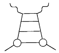
Figure 11: Example of ladder graph with several rungs.

We now decompose the complete structure function as

$$F = \sum_{N=0}^{\infty}G_{s}\,G_{r}^{N}\,G_{h}$$ (94)

$$= G_{s}\,\frac{1}{1-G_{r}}\,G_{h}.$$

Here $G_{s}$ is the sum of all two-particle-irreducible graphs attached to the initial state particle, $G_{h}$ is the sum of all two-particle-irreducible graphs coupling to the virtual photon, and $G_{r}$ is the sum of all graphs for a rung of the ladder. Thus $G_{r}$ is the sum of all two-particle-irreducible graphs with two upper lines and two lower lines, multiplied by full propagators for the upper lines.

The second line of Eq. (94) has the inverse of $1-G_{r}$, and it clearly suggests a kind of operator or matrix formalism. Indeed, if we make explicit the external momenta of two ladder graphs, $\gamma_{1}(k,l)$ and $\gamma_{2}(k,l)$, then their product is

$$(\gamma_{1}\gamma_{2})(k,l)=\int\frac{{\rm d}^{6-\epsilon}k^{\prime}}{(2\pi)^{6-\epsilon}}\gamma_{1}(k,k^{\prime})\gamma_{2}(k^{\prime},l).$$ (95)

The rung graphs can thus be treated as matrices whose indices have a continuous instead of a discrete range of values, while $G_{s}$ and $G_{h}$ can be treated as row- and column-vectors.

In the case that the initial hadron is a single parton, as in the low order examples in Sect. 5, the soft part $G_{s}$ is trivial: $G_{s}=1$, where ‘1’ represents the unit matrix.

6.2 Extraction of higher twist remainder

We can now symbolize the operations used to extract the contribution of a graph to the hard scattering coefficient. Consider the example that lead to Eq. (83). We took the original graph and subtracted the contribution of the graph to $f^{(1)}H^{(0)}$, where $H^{(0)}$ is the lowest order hard part. Then we took the large $Q$ asymptote of the result, by setting all the masses to zero.

Figure 12: Hard scattering coefficient from Fig. 6(a).

We represent this in a graphical form in Fig. 12. There, the wavy line represents the operation of short circuiting the minus and transverse components of the loop momentum coming up from below, and of setting all masses above the line to zero. Symbolically, we write this as:

Contribution of Fig. 6(a) to $$H^{(1)} = P\gamma\gamma_{h}-P\gamma P\gamma_{h}$$ (96)

$$= P\gamma\,(1-P)\,\gamma_{h},$$

where the operator $P$ is defined by

$$\begin{split}P(k,l){}={}&(2\pi)^{6-\epsilon}\,\delta(k^{+}-l^{+})\,\delta(l^{-})\,\delta^{6-\epsilon}({l_{\perp}})\\ &{}\times{}(\mbox{Set masses to zero in the part of the graph above $P$}).\end{split}$$ (97)

In Eq. (96) we have ignored the need for renormalization that occurs if $\epsilon=0$. Either we can assume that we are only making the argument when $\epsilon$ is slightly positive, or assume that all necessary renormalization is implicitly performed by minimal subtraction.

Figure 13: Contribution of Fig. 6(a) to $f^{(1)}H^{(0)}$.

Fig. 6(a) gives two contributions to the factorization: a contribution to the one-loop hard part $H^{(1)}$ given in Eq. (96) or (83), and a contribution to $f^{(1)}H^{(0)}$. The second of these we picture in Fig. 13 and symbolize as

$$\gamma P\gamma_{h}.$$ (98)

Thus we can write the remainder for Fig. 6(a), after subtracting its leading twist contribution, as

$${\rm Rem}(\mbox{Fig.\ \ref{fig:6}(a)}) = \gamma\gamma_{h}\,-\,\gamma P\gamma_{h}\,-\,P\gamma(1-P)\gamma_{h}$$ (99)

$$= (1-P)\gamma(1-P)\gamma_{h}.$$

Clearly the operator $1-P$ subtracts out the leading behavior.

In general, we can write the remainder for the complete structure function as

$$F_{\rm Rem} = \sum_{N=0}^{\infty}G_{s}\,[(1-P)G_{r}]^{N}\,(1-P)\,G_{h}$$ (100)

$$= G_{s}\,(1-P)\,\frac{1}{1-G_{r}(1-P)}\,G_{h}.$$

This formula is valid without renormalization, even at $\epsilon=0$. In the first place, renormalization of the interactions can be done inside the $\gamma$’s. This is because there is nesting but no overlap between, on the one hand, the graphs to which the operation $1-P$ is applied and, on the other hand, the vertex and self-energy graphs for which counterterms are needed in the Lagrangian of the theory. Further divergences occur because of the extraction of the asymptotic behavior, and these give rise to the need to renormalize the parton distribution. But the regions that give rise to such divergences are of the form where lines in some lower part of a graph are collinear relative to lines in the upper part. All such regions are canceled in Eq. (100) since to the operator $1-P$ they behave just like the regions that give the leading twist behavior of the structure function.

6.3 Factorization

It is now almost trivial to prove factorization for the leading twist part of the structure function, which is

$$F-F_{\rm Rem}=G_{s}\,\frac{1}{1-G_{r}}\,G_{h}-G_{s}\,(1-P)\,\frac{1}{1-G_{r}(1-P)}\,G_{h}.$$ (101)

Simple manipulations give

$$F-F_{\rm Rem} = G_{s}\,\frac{1}{1-G_{r}}P\frac{1}{1-G_{r}(1-P)}\,G_{h}$$ (102)

$$= f*H.$$

We now have an explicit formula for the hard scattering coefficient:

$$H=P\,\frac{1}{1-G_{r}(1-P)}\,G_{h},$$ (103)

while the parton distribution $f$ satisfies

$$f\times P=G_{s}\,\frac{1}{1-G_{r}}\,P.$$ (104)

One somewhat unconventional feature of our procedure is that not only do we define $P$ to set to zero the minus and transverse components of the momenta going into the subgraph above it, but we also define it to set masses to zero. Setting the minus and transverse momenta to zero while preserving the plus component is exactly the appropriate generalization of BPH(Z) zero-momentum subtractions to the present situation. Setting the masses to zero as well is a convenient way of extracting the asymptotic large-$Q$ behavior of a graph, as we saw in our explicit calculations. Moreover, particularly in QCD, it greatly simplifies calculations if one works with a purely zero-mass theory. Of course, setting masses to zero gives infrared divergences in all but purely ultraviolet quantities. The momentum-space regions that give the divergences associated with the structure function all have the same form as the leading regions for large $Q$, Fig. 9, so that the $1-P$ factors in Eq. (104) kill all these divergences. Note that, just as with Zimmermann’s methods, the $P$ operator can be applied at the level of integrands. In practical calculations, dimensional continuation serves as both an infrared and an ultraviolet regulator.

In the one-loop example of Sect. 5, the external hadron is a parton, so that in $G_{s}=\delta(x-1)$ in (104). At one loop, $G_{r}$ corresponds exactly to $f_{c}$, Eq. (80). This expression, and the distribution $f$ as a whole in (104) is still unrenormalized, and contains ultraviolet divergences. These may be removed by minimal subtraction, as in Eq. (81) at one loop, or as discussed more generally in Ref. [10]. We should mention, however, that it would be advantageous to have a subtraction procedure which combined factorization and renormalization into a single operation. The particular procedure outlined by Zimmermann [3] does this, but is not immediately applicable when all particles are massless. Duncan and Furmanski [19] have discussed some of these issues at length.

6.4 Factorization for Inclusive Annihilation in ${(\phi^{3})}_{6}$

It is easy to generalize the general arguments of this and the previous section to other processes, such as those listed in the introduction. An important example, is the cross section in $\phi^{3}$ theory that is analogous to one-particle inclusive annihilation in $e^{+}e^{-}$ annihilation, that was discussed in Sect. 1.2. In the scalar theory, the structure function for this process is

$$D(x,Q)=\frac{Q^{2}}{2\pi}\int{\rm d}^{6}y\,e^{iq\cdot y}\sum_{X}\langle 0|j(y)|HX\rangle\langle HX|j(0)|0\rangle,$$ (105)

which is exactly analogous to the QCD version, Eq. (6).

It is relatively easy to check that the leading regions for this process have a form that generalizes Fig. 9 for deeply inelastic scattering, that is, they have the form of Fig. 14. This was shown in Ref. [20] (for the case of a non-gauge theory).

Figure 14: Example of leading region for inclusive annihilation. Regions with more than one jet inside the hard subdiagram $H$ are also leading.

An example is given by the ladder graph of Fig. 15. We must integrate over all values of the momentum $(k-p)^{\mu}$. When $(k-p)^{\mu}$ is collinear to $p^{\mu}$, the line $k$ has low virtuality. Then in the overall center-of-mass, the remaining particle $q-k$ has large energy, approximately $Q/2$, and is moving in the opposite direction to the first two particles. We therefore consider the lines $p$, $k-p$ and $k$ as forming the jet $J_{A}$ in Fig. 14 and $q-k$ together with the vertex where the ‘virtual photon’ attaches as forming the hard part $H$. When $(k-p)^{\mu}$ has transverse momentum of order $Q$, we put both $k$ and $k-p$ into the hard part.

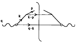
Figure 15: Ladder graph.

In a non-gauge theory, these two regions are the only significant ones, together with a region that interpolates between them. As we shall see in Sect. 7, this statement generalizes to all orders of perturbation theory. In a gauge theory, like QCD, all kinds of complication arise because there are also ‘leading twist’ regions involving soft gluons.

6.5 Factorization, fragmentation function

Simple generalizations of the arguments for deeply inelastic scattering give the scalar factorization theorem:

$$D(z,Q)=\int_{z}^{1}\frac{{\rm d}\zeta}{\zeta}\,H(z/\zeta,Q)\,d(\zeta)+{\cal O}(1/Q^{a}).$$ (106)

analogous to Eq. (7). Here the fragmentation function is defined in exact analogy to the parton distribution. We choose axes so that the momentum $p^{\mu}$ of the detected particle is in the positive $z$-direction. Then we define:

$$d(z) = \frac{p^{+}}{2\pi z}\int{\rm d}y^{-}e^{ip^{+}y^{-}/z}\sum_{X}\langle 0|\phi(0,y^{-},0_{T})|HX\rangle\langle HX|\phi(0)|0\rangle$$ (107)

$$= \frac{p^{+}}{z}\int\frac{{\rm d}k^{-}{\rm d}^{4}k_{T}}{(2\pi)^{6}}\Phi_{D}(k,p).$$

This is interpreted as the number density of hadrons $H$ in a parton. The formulae are exactly analogous to Eqs. (75) and (78) for the parton distribution. Renormalization is needed here also.

7 Leading Regions

As we saw in Sects. 5 and 6, the first step in constructing a complete proof of a factorization theorem is to derive the leading regions of momentum space for a graph of arbitrary order. This section begins with a brief description of a general approach to the long- and short-distance behavior of Feynman diagrams that results in a derivation of the leading regions. We apply this method to describe the origin of high-energy logarithms in scalar theories, and go on to discuss the cancellation of final state interactions, and the infrared finiteness of jet cross sections.

7.1 Mass dependence and leading regions

Consider, then, an arbitrary Feynman integral $G({p_{i}^{\nu}}/\mu,m/\mu)$, corresponding to a graph $G$, which is a function of external momenta $p_{i}^{\nu}$, mass $m$ (possibly zero), and renormalization scale $\mu$. Without loss of generality, we may take $G$ to be dimensionless. We also assume that the invariants formed from different $p_{i}^{\nu}$ are all large, while the $p_{i}^{\nu}$ themselves have invariant mass of order $m$. Thus:

$$p_{i}\cdot p_{j}=Q^{2}\eta_{ij},\ \ p_{i}^{2}=\zeta_{i}m^{2},$$ (108)

where $Q$ is a high-energy scale, $Q\gg m$, and the $\eta_{ij}$ and $\zeta_{i}$ are numbers of order unity. In the following, it will not be necessary to consider the $\eta_{ij}$ and $\zeta_{i}$ dependence, and we will write $G$ as $G(Q^{2}/\mu^{2},m^{2}/\mu^{2})$. We will be interested in the leading term in an expansion in powers of $1/Q^{2}$. (Always we will allow the possibility of a polynomial in $\ln Q$ multiplying the power of $Q$, in each order of perturbation theory.)

Suppose $G$ is the result of $L$ loop momentum integrations acting on a product of $I$ Feynman propagators, times a function $N$, which is a polynomial in the internal and external momenta. For simplicity, we absorb into $N$ the numerator factors associated with the internal propagators, as well as overall kinematic factors, etc. $G$ may then be represented schematically as

$$G(Q^{2}/\mu^{2},m^{2}/\mu^{2})=\prod_{i=1}^{L}\int{\rm d}^{n}\ell_{i}\ N(\{k_{j}\},\{p_{i}\})\prod_{j=1}^{I}\frac{1}{(k_{j}^{2}-m^{2}+i\epsilon)}.$$ (109)

The line momenta $\{k_{j}^{\mu}\}$, of course, are functions of the $\ell_{i}^{\mu}$ and the $p_{i}^{\mu}$. Any region in $\ell^{\mu}$ space which contributes to $G$ at leading power in $Q^{2}$ will be called a “leading region”. In addition, by a “short-distance” contribution to (109) we will mean that we have a region of loop momenta in which some subset of the line momenta, $\{k_{j}^{\mu}\}$, are off-shell by at least ${\cal O}(Q^{2})$; the short-distance contribution is the factor in (109) given by these far off-shell lines. Short-distance contributions are independent of masses to the leading power in $Q^{2}$, since the integrand can usefully be expanded in powers of $m^{2}$ when propagators are far off-shell. A general leading region has both short-and long-distance contributions, the latter associated with lines which are nearer the mass shell. Roughly speaking, factorization is the statement that the cross section is a product of parton distributions, in which all the long-distance contributions are found, and a hard-scattering coefficient, which has purely short-distance contributions. To study factorization, we must characterize all “long- distance” contributions.

Our analysis depends on two observations. The first concerns the close relation between the high-energy and zero-mass limits. That is, if the renormalization scale $\mu$ is chosen to be of ${\cal O}(Q)$, then the two limits are equivalent in the function $G(1,m^{2}/Q^{2})$. Short-distance contributions to the $Q\to\infty$ limit are those involving lines for which $k_{j}^{2}$ is of order $Q^{2}$. Long-distance contributions are parts of the $\ell_{i}^{\mu}$ integrations for which $k_{j}^{2}$ is much less than $Q^{2}$. If we scale all momenta down by a factor proportional to $Q$, then we are considering the $m\to 0$ limit instead. The short-distance contributions now have fixed $k_{j}^{2}$ and the long-distance contributions have Feynman denominators $k_{j}^{2}+i\epsilon$ in Eq. (109) that vanish in the $m\to 0$ limit.

Note that if $G$ is such that it only has short distance contributions, then the $Q\to\infty$ limit is $G(1,0)$, i.e., we can just set $m=0$. The QCD coupling, $\alpha_{s}(Q)$, is an implicit argument for $G$, and we have already chosen to set the renormalization scale $\mu$ equal to $Q$. Thus in this case the detailed large $Q$ behavior is renormalization-group controlled in a simple way.

When there are long-distance contributions to $G$, an expansion in powers of $m$ will often fail. So to find the long-distance contributions to $G$, one must look for singularities in the $m\to 0$ limit. There are apparent exceptions to this rule, exemplified by the integral

$$\int_{0}^{\infty}{\rm d}k^{2}\frac{m^{2}}{(k^{2}+m^{2})^{2}}.$$ (110)

However, if we factor out the numerator factor $m^{2}$, we are left with an integral that is singular like $1/m^{2}$. This singularity is governed by the denominator. So what we are looking for is singularities in the $m$ dependence in the integral over the denominators of $G$.

Our second observation is that the integrals in (109) are defined in complex $\ell_{i}^{\mu}$-space. As a result, it is not enough for a set of denominators to vanish in the integrand of (109) for the integral to produce a singularity at $m=0$ in $G$. We must have, in addition, a pinch of one or more of the $\ell_{i}^{\mu}$ integrals at the position of the singularity, between coalescing poles. This fact enables us to apply the simple but powerful analysis due originally to Landau [21, 22] on the relation of singularities in Feynman integrands to the singularities of Feynman integrals. In the next subsection we explain the application of this argument.

7.2 Pinch surfaces

We begin by using Feynman parameterization to combine the denominators of Eq. (109) by

$$G(Q^{2}/\mu^{2},m^{2}/\mu^{2}) = (I-1)!\,\prod_{j=1}^{I}\int_{0}^{1}{\rm d}\alpha_{j}\,\delta\!\!\left(1-\sum_{j=1}^{I}\alpha_{j}\right)\prod_{i=1}^{L}\int{\rm d}^{n}\ell_{i}\$$ (111)

$$\times\frac{N(\{k_{j}\},\{p_{i}\})}{\left[\sum_{j=1}^{I}\alpha_{j}(k_{j}^{2}(\ell_{i}^{\nu})-m^{2})+i\epsilon\right]^{I}},$$

where we have exhibited the loop-momentum dependence of the line momenta. There is now a single denominator $D(\ell_{i},\alpha_{j})$, which is quadratic in loop momenta and linear in Feynman parameters. Suppose $D(\ell_{i},\alpha_{j})$ vanishes for some value of loop momenta and Feynman parameters. We will now derive necessary conditions for this zero to produce a singularity in $G$. Then we will apply these conditions to the case $m=0$.

A pole from $D=0$ will not give a singularity in $G$ if $D$ can be changed from zero by a deformation that does not cross a pole in any one of the momentum or parameter contours. Consider first the parameter integrals. Because $D$ is linear in the $\{\alpha_{j}\}$, a deformation of the $\alpha_{j}$ integral will change $D$ away from zero, unless

$$k_{j}^{2}=m^{2}\ \ {\rm or}\ \ \alpha_{j}=0$$ (112)

for each line. In the first case, $D$ is independent of $\alpha_{j}$, while in the second we note that $\alpha_{j}=0$ is an endpoint of the $\alpha_{j}$ integral, away from which it cannot be deformed.

Now suppose (112) is satisfied, and consider the momentum integrals. $D$ will be independent of those loop momenta which flow only through lines whose Feynman parameters are zero. The contours of the remaining loop momenta must be pinched between singularities associated with the vanishing of $D$. Since $D$ is a quadratic function of the remaining momenta, each momentum component sees only two poles in its complex plane due to the vanishing of $D$. The condition for a pinch is thus the same as the condition that the two zeros of the quadratic form be equal. That is, in addition to $D=0$ we must have $\partial D/\partial\ell_{i}^{\mu}=0$ for all $\ell_{i}^{\mu}$ which flow through one or more on-shell lines. For each such loop momentum, the extra condition is [21, 22]

$$\sum_{j}\alpha_{j}k_{j}^{\mu}=0,$$ (113)

where the sum goes over all lines through which the loop momentum $\ell_{i}^{\mu}$ flows. (Note that any line which is not on shell has $\alpha_{j}=0$, by Eq. (112), so the condition (113) can be applied to every loop.) Together, (112) and (113) are known as the “Landau equations”. We shall refer to any surface in momentum space on which the Landau equations are satisfied as a “pinch surface” of the diagram $G$. With each pinch surface we associate a “reduced diagram”, in which all off-shell lines are shrunk to points. By construction, the reduced diagram contains only those loop momenta of the original diagram which satisfy (113) with nonzero $\alpha$’s.

7.3 Physical propagation

The Landau equations are surprisingly restrictive, especially in the zero-mass limit. To see why, let us rederive the observation of Coleman and Norton [23, 24] that Eqs. (112) and (113) have an appealing physical interpretation. Consider a given pinch surface. We rewrite (113) on this surface as

$$\sum_{j}(\alpha_{j}\ \omega_{j})v_{j}^{\mu}=0,$$ (114)

where $v_{j}^{\mu}$ and $\omega_{j}$ are the four-velocity and energy associated with the momentum $k_{j}^{\mu}$. The units of the Feynman parameters are arbitrary, so suppose we may, if we wish, interpret $\alpha_{j}$ as the frame-independent ratio of a time to the energy of line $j$. Then each of the components of the vector $(\alpha_{j}\omega_{j})v_{j}^{\mu}$ has the units of a distance in space-time. It is the distance traversed in time $(\alpha_{j}\omega_{j})$ by a free particle moving classically with velocity $v^{\mu}_{j}$.

Now suppose we associate a definite position $x_{1}^{\mu}$ to one of the vertices in the reduced diagram associated with the pinch surface. Then, if line $j$ attaches to the vertex at $x_{1}^{\mu}$, $x_{1}^{\mu}+(\alpha_{j}\ \omega_{j})v_{j}^{\mu}$ may be interpreted as the position of the vertex at the other end of line $j$. Continuing in this manner, we can associate with the reduced diagram a position in space-time for every one of its vertices, and a physical process in which free particles move between these points. Equation (113) ensures that this program can be carried out consistently, by requiring that in going around any closed loop we come back to the same position. We can use this construction as a necessary condition for a pinch surface.

Finally, note that, because Eqs. (112) and (113) are homogeneous in the $\alpha$’s, a rescaling of the $\alpha$’s leaves the Landau equations satisfied. Hence the vertices in the physical picture are an indefinite distance apart, and, in particular, this distance may be arbitrarily large.

7.4 Collinear and infrared pinches; power counting

For a general diagram with arbitrary masses and external momenta the criterion of physical propagation allows a very rich analytic structure. In the massless limit, however, this structure actually simplifies since multiparticle thresholds become degenerate. The physical processes of which an isolated massless (but not massive) particle is kinematically capable are as follows. First, a massless particle of momentum $p^{\mu}$ may split into two (or more) massless particles of momenta $\alpha p^{\mu}$ and $(1-\alpha)p^{\mu}$, and vice-versa. This is the source of collinear divergences. Second, a particle may emit or absorb one (or more) zero energy particles. This is the source of infrared divergences. We easily check that arbitrary loops involving only collinear and zero-momentum particles can satisfy the Landau equations. Generally, we will describe a subdiagram consisting of mutually collinear particles as a “jet” subdiagram. Lines that have zero momentum in the massless limit we will call “infrared”. A jet subdiagram describes the evolution of a set of collinear lines, as they absorb and emit other collinear and infrared lines.

As an example, let us consider the vertex correction Fig. 16a, in dimensionally regulated $\phi^{3}$ theory,

$$V(p,p^{\prime})=\int\frac{{\rm d}^{n}k}{(2\pi)^{n}}\ \frac{1}{[(p^{\prime}-k)^{2}-m^{2}+i\epsilon]\,[(p+k)^{2}-m^{2}+i\epsilon]\,(k^{2}-m^{2}+i\epsilon)},$$ (115)

where we assume a production process, $Q^{2}\equiv(p^{\prime}+p)^{2}>0$. This example is used for illustrative purposes only. The term “leading” will refer here only to this diagram, and not to the behavior of the Born diagram. In fact, Fig. 16(a) is nonleading compared to the Born process for all $n<6$.

The Landau equation for Fig. 16(a) is

$$\alpha_{1}(p^{\prime}-k)^{\mu}+\alpha_{2}(p+k)^{\mu}+\alpha_{3}k^{\mu}=0.$$ (116)

For on-shell ($p^{2}={p^{\prime}}^{2}=m^{2}$) scattering with $m\neq 0$, Eq. (116) has no solutions at all. Note that this is the case even though there is a singular surface illustrated in Fig. 16(b), with

$$(p+k)^{2}=(p^{\prime}-k)^{2}=m^{2},\ k^{2}<0.$$ (117)

This singular surface corresponds to the production of two particles, followed by a subsequent spacelike scattering. Although such a process is kinematically possible, it clearly cannot correspond to physical propagation, because the two particles produced at vertex $1$ propagate in different directions, and would therefore not be able to meet at vertex $2$ to scatter again.

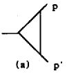
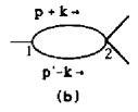
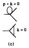
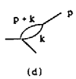
Figure 16: (a) Vertex correction, (b) Reduced diagram corresponding to Eq. (117), (c) Infrared reduced diagram, (d) collinear reduced diagram.

Now let us consider the case that $m=0$. By the same reasoning, (117) does not give a pinch surface, if $k\neq 0$. There are nevertheless two sets of solutions. First, there are infrared solutions where one line has zero momentum,

$$k^{\mu}=0, ~{}~{}\alpha_{1}=\alpha_{2}=0,$$

$$(p+k)^{\mu}=0, ~{}~{}\alpha_{1}=\alpha_{3}=0,$$

$$(p-k)^{\mu}=0, ~{}~{}\alpha_{2}=\alpha_{3}=0.$$ (118)

Second, there are collinear solutions, where two of the lines are parallel to one of the outgoing external particles,

$$\alpha_{1}(p-k)^{\mu}+\alpha_{3}k^{\mu} =0,~{}\alpha_{2}=0,\ k^{2}=p\cdot k=0,$$

$$\alpha_{2}(p^{\prime}+k)^{\mu}+\alpha_{3}k^{\mu} =0,~{}\alpha_{1}=0,\ k^{2}=p^{\prime}\cdot k=0.$$ (119)

The physical pictures associated with typical infrared and collinear pinch surfaces are shown in Figs. 16(c) and (d), respectively. In each case, there is physically realizable propagation between vertices.

Now we observe that even though solutions to the Landau equations like Eqs. (118) and (119) give pinch surfaces, they still do not necessarily produce mass dependence that is relevant to the leading power of $Q$, and hence are not necessarily leading regions.

The Born graph for the vertex behaves like $Q^{0}$. The contribution to the one-loop graph from the pure short-distance region, from the region, $|k^{\mu}|={\cal O}(Q)$, is $Q^{n-6}$. Thus this region is leading when the theory is renormalizable, at $n=6$, but is non-leading relative to the Born graph when the theory is super-renormalizable, $n<6$.

Next we consider the one-loop graph near its singular surfaces. For example, consider the integral (115) near the surface defined by the first of Eqs. (118). To be specific, let $|k^{\mu}|<k_{\rm max}$, $\mu=0\cdots 3$, with $k_{\rm max}$ being some fixed scale (which must $\gtrsim m$). In this region the integral behaves as

$$\frac{1}{Q^{2}}\int_{k^{\mu}<k_{\rm max}}\frac{{\rm d}^{n}k}{k^{4}}\sim\frac{k_{\rm max}^{n-4}}{Q^{2}}.$$ (120)

Compared to the short-distance region, this infrared region is leading only for $n\leq 4$. (The other two infrared regions in (118) require $n\leq 2$.) (We remind the reader that, compared to the Born graph, none of these regions contribute to the leading power of $Q$.)

Similarly, near the collinear pinch surfaces of Eq. (118), the integral behaves as

$$\frac{1}{Q^{2}}\int_{k_{\perp}<k_{\rm max}}\frac{{\rm d}k^{2}}{k^{2}}\frac{{\rm d}^{n-2}k_{\perp}}{k_{\perp}^{2}}\ \sim\frac{k_{\rm max}^{n-4}}{Q^{2}},$$ (121)

so that again only for $n\leq 4$ do we find collinear contributions from this diagram that are leading compared with the short-distance contribution.

In summary, for the scalar theory in six dimensions, only short distance regions are (relatively) leading for Fig. 16. This result generalizes to all orders in the vertex correction for this theory [25].

The process of estimating the strength of a singularity is known as “power counting”. We will give more low order examples below, while more general arguments can be found in Ref. [24]. We can, however, summarize the basic result of these arguments briefly. Let $D$ be a reduced diagram with $S$ “infrared loops” and $I_{S}$ infrared lines whose momenta vanish at the corresponding pinch surface, and with $C$ “collinear loops” and $I_{C}$ collinear lines whose momenta become proportional to an external momentum at the pinch surface. Finally, let $N_{2}$ denote the number of two point subdiagrams in $R$. In $\phi^{3}$ theory in $n$ space-time dimensions, let us define [24] the “degree of divergence” by

$$\omega(R)=nS+(n/2)C-2I_{S}-I_{C}+N_{2}.$$ (122)

This corresponds to a power law

$$Q^{(n-6)V}\lambda^{\omega(R)}$$ (123)

as $Q\to\infty$. Here $V$ is the number of loops and $\lambda$ is a small parameter that parameterizes the approach to the singularities in the massless theory. The power law is measured relative to the power for the Born graph.

In the renormalizable case, $n=6$, we get leading behavior only if $\omega(R)=0$ and there are no graphs that give negative $\omega(R)$. The term $N_{2}$, which tends to suppress the behavior of the integral at the singular point, is due to the fact that the renormalized two-point function must vanish on-shell if the particle is to have zero mass. In this sense, the infrared behavior of the theory is dependent on renormalization [24].

In the superrenormalizable case, $n<6$, the first factor in (123) gives a negative power of $Q$ that just corresponds to normal ultraviolet power counting; this is the power that comes from a purely short-distance contribution to the graph. A sufficiently strong power law singularity in the massless theory is needed to overcome this if one is to get a leading contribution.

7.5 Leading regions for deeply inelastic scattering in ${(\phi^{3})}_{6}$

As an application, we now discuss the general leading regions for the basic inclusive cross sections in ${(\phi^{3})}_{6}$. The criterion of physical propagation shows why the considerations of Sects. 5 and 6 take into account all relevant leading regions. To see this, we must generalize our concept of leading regions to include cut diagrams, of the type discussed in Sects. 5 and 6. There is no problem in doing this, and power counting may be estimated for collinear and infrared cut lines with the same degree of divergence Eq. (122) as for virtual lines.

It is useful to apply the optical theorem to reexpress the deeply inelastic scattering structure function Eq. (63) as the discontinuity of the forward Compton scattering amplitude $T(q,p)$,

$$F(x,Q^{2}) = \mathop{\rm disc}T(q,p),$$

$$T(q,p) = \frac{Q^{2}}{2\pi}\int{\rm d}^{6}y\,e^{iq\cdot y}\langle p|T(j(y)j(0)|p\rangle.$$ (124)

This relation holds diagram-by-diagram, once cuts are summed over, so that a necessary condition for a region $L$ to be leading in $F$ is that it be leading in $T$.

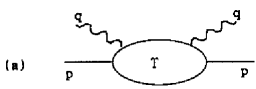
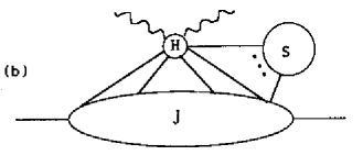
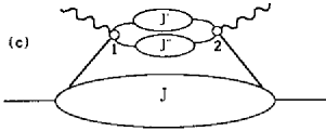
Figure 17: (a) Diagrams for forward Compton scattering. (b) Reduced diagrams for pinch surfaces. (c) Reduced diagram for a singular surface which is not pinched.

We thus need to consider the leading regions of the diagrams illustrated by Fig. 17(a), which represents forward Compton scattering. The pinch surfaces are symbolized in Fig. 17(b). The incoming hadron can form a jet of lines, and in addition, may interact with any number of soft lines, connected to a subdiagram $S$ consisting of only lines with zero momentum. To see why this is the general form, consider a singular surface not of this kind, as in Fig. 17(c). Here, one or more lines of the jet may scattering with the incoming photon to form a set of on-shell outgoing jets, which then rescatter to emit the outgoing photon and reform the outgoing jet, which eventually evolves into the outgoing hadron. Such a process is certainly consistent with momentum conservation. Surfaces of this type are not pinch surfaces for the amplitude $T(q,p)$, however, because the outgoing jets can never collide again once they have gone a finite distance from the point at which they are produced. As a result, in every pinch surface, the incoming and outgoing photons attach at the $same$ point in space-time, and we derive the picture of Fig. 17(b). This result shows that all divergences associated with final state interactions cancel in the sum over final states.

As indicated above, not every pinch surface will correspond to a leading region. In particular, power counting using Eq. (122) shows that there are no infrared divergences in ${(\phi^{3})}_{6}$, that is, no zero-momentum lines for any leading region [24]. In addition, we can show that only the minimum number of jet lines (two) can attach the jet to the hard part in Fig. 17(b). It is a straightforward exercise in counting to prove these results, using (122), the Euler identity (loops = lines - vertices + 1), and the observation that every internal line of a graph begins and ends at a vertex. In summary, we can show that Fig. 9 is indeed the reduced diagram of the most general leading region for deeply inelastic scattering in the scalar theory.

7.6 Unitarity and jets: the cancellation of final state interactions

The cancellation of final state interactions in deeply inelastic scattering plays an important role in the analysis for deeply inelastic scattering just described. This cancellation is a general feature of inclusive hard scattering cross sections, and is used repeatedly in factorization proofs. The physics behind this cancellation has already been pointed out in Sect. 5: a hard scattering is well localized in space-time, and, as a result, it cannot interfere with long-distance effects which describe the further evolution of the system. Thus, when we sum over final states in an inclusive cross section, we lose information on the details of evolution in the final state, and are left with the constraint that, by unitarity, the sum of probabilities of $all$ final states is unity. As a result, at each order in perturbation theory, long-distance contributions to final states must cancel.

It is worth noting that it is not always necessary to sum over all final states to cancel long-distance interactions. There are three kinds of cross sections, among those mentioned in Sect. 1, for which the cancellation of final state interactions is important. In deeply inelastic scattering and Drell-Yan, for instance, we sum over all hadronic final states. In single-particle inclusive cross sections, on the other hand, we shall find in Sect. 9 that cancellation requires the use of Ward identities. Finally, in jet cross sections, the cancellation comes about in a sum over all final states which satisfy certain criteria in phase space. Let us hint at how this happens.

If all non-forward particles in the final state emerge from a single hard scattering, the criterion of physical propagation requires that the long-distance contributions will come entirely from soft and collinear interactions. This is because, as in the low order example of Fig. 16, jets emerging from a single point and propagating freely cannot meet again to produce a new hard scattering. In this case, once the energy and direction of a set of jets is specified, the sum over only those final states consistent with these jets will also give unity, and their collinear and infrared divergences cancel in the sum. The technical proof of these statements may be given in a number of ways. The simplest is based on a truncation of the hamiltonian to describe only collinear and infrared interactions. Then, since the truncated hamiltonian is hermitian, it generates a unitary evolution operator whose divergences cancel by the “KLN” theorem [26, 27]. It is also useful to see that this cancellation is manifested on a diagram-by-diagram basis within each leading region in perturbation theory [24]. Proofs of this type are most easily given in terms of time-ordered or light-cone ordered perturbation theory [11, 28].

Technicalities aside, the cancellation of final state interactions at the level of jets has a number of important consequences. The simplest of these is the finiteness of jet cross sections in $e^{+}e^{-}$-annihilation cross sections [29]. We have already seen its importance for the analysis of deeply inelastic scattering in ${(\phi^{3})}_{6}$. It has a similar simplifying effect for single-particle inclusive cross sections, as well as for the Drell-Yan and related cross sections. To illustrate this, we show, in Fig. 18 the reduced diagrams for leading regions in the scalar “Drell-Yan” cross section, defined for the scalar theory by analogy to Eq. (63) in ${(\phi^{3})}_{6}$, after the sum over final states. We see that all information about the final state has been absorbed into a single hard part $H$. Note that this result holds not only for the fully inclusive Drell-Yan cross section, but also for semiinclusive cross sections such as hadron-hadron $\rightarrow$ Drell-Yan pair + jets.

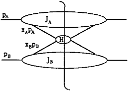
Figure 18: Leading regions for the Drell-Yan cross section in ${(\phi^{3})}_{6}$.

8 Factorization and Gauge Invariance

In this and the following section, we discuss the extension of factorization proofs to gauge theories. We begin with a discussion of the classical Coulomb field of a fast moving charge, an example that anticipates what happens in the full quantum theory.

We next summarize the Ward identities we will need. Then we discuss the leading regions of Feynman graphs in a gauge theory. There are great differences from the case of the $\phi^{3}$ theory discussed in the previous section. With the aid of the example of the vertex graph, we show how, after an appropriate eikonal approximation, Ward identities are applicable that will combine graphs into a factorized form.

In the next section, we will show how factorization may be proved for a variety of experimentally important cross sections, which can be measured in deeply inelastic scattering, $e^{+}e^{-}$ annihilation and hadron-hadron scattering. We should emphasize at the outset that although we regard existing proofs in all these cases as reasonably satisfying, there is still room for improvement, especially for hadron-hadron cross sections. We will point out the shortcomings of existing arguments in Sect. 10.

8.1 Classical considerations

Before getting into a detailed discussion of Feynman diagrams, it is worth noting that insight can be gained into the physical content of factorization theorems from purely classical considerations. This discussion will at once highlight an important difference between gauge and scalar theories, and at the same time show why this difference, important though it is, respects factorization.

As we observed in Sect. 1.4, the parton model picture of hadron-hadron scattering rests in part on the Lorentz contraction of colliding hadrons. Now a simplified classical analog of a hadron is a collection of point charges, each acting as a source of a classical scalar field. We would expect that if the parton model, or factorization, is to make sense, these fields ought to be Lorentz contracted themselves, and this is just what happens. Let us see how.

Consider first a static classical scalar field $\phi_{\rm cl}({\bf x})$, associated with a point particle of charge $q$ at the origin. If we assume that the field obeys Laplace’s equation, it is given in the rest frame of the particle by

$$\phi_{\rm cl}({\bf x})=\frac{q}{|{\bf x}|}.$$ (125)

Now consider the same field in a frame where the particle is moving at velocity $c\beta$ along the $z$-axis. Then the field at ${x^{\prime}}^{\mu}$ in this frame is

$$\phi_{\rm cl}^{\prime}(x^{\prime})=\frac{q}{\bigl{[}x_{T}^{2}+\gamma^{2}(\beta ct^{\prime}-x^{\prime}_{3})^{2}\bigr{]}^{1/2}},$$ (126)

where, as usual, $\gamma=(1-\beta^{2})^{-1/2}$. For an observer at $t^{\prime}=0$ in the primed system, the $\phi$ field decreases as $\gamma^{-1}$ as $\beta$ approaches unity, except near $x^{\prime}_{3}=0$. Thus, the $\phi$ field is indeed Lorentz contracted, and any force proportional to the $\phi$ field is also Lorentz contracted into a small longitudinal distance about $x^{\prime}_{3}=0$. This means that in the rest frame of a scalar “hadron”, the forces due to another such hadron approaching at nearly the speed of light are experienced in a Lorentz-contracted fashion, just as supposed in the parton model.

Now let us apply this reasoning to a classical gauge theory, in this case classical electrodynamics. Here, the field in the rest frame of a point particle of charge $q$ is precisely analogous to Eq. (125),

$$A_{\rm cl}^{\mu}({\bf x})=\frac{q\delta_{\mu 0}}{|{\bf x}|}.$$ (127)

Because this is a vector field, however, there is a big difference from the scalar case in a frame in which the particle moves with velocity $c\beta{\hat{\bf x}}_{3}$. In this frame, we find

$${A^{\prime}_{\rm cl}}^{0}(x^{\prime}) = \frac{q\gamma}{\left[{x_{\perp}}^{2}+\gamma^{2}(\beta ct^{\prime}-x^{\prime}_{3})^{2}\right]^{1/2}},$$

$${A^{\prime}_{\rm cl}}^{3}(x^{\prime}) = \frac{-q\beta\gamma}{\left[{x_{\perp}}^{2}+\gamma^{2}(\beta ct^{\prime}-x^{\prime}_{3})^{2}\right]^{1/2}},$$

$${A^{\prime}_{\rm cl}}_{T}(x^{\prime}) = 0.$$ (128)

For large $\gamma$, the field in the zero and three directions are actually independent of $\gamma$ at fixed times before the collision. It might therefore seem that a vector field is not Lorentz contracted, and would not respect the assumptions of the parton model. If we look, however, at the field strengths rather than the vector potential, we find a different story. The electric field in the three direction, for instance, is given in the primed frame by

$$E_{3}^{\prime}(x^{\prime})=\frac{-q\gamma(\beta ct^{\prime}-x_{3}^{\prime})}{\bigl{[}{x_{\perp}}^{2}+\gamma^{2}(\beta ct^{\prime}-x_{3}^{\prime})^{2}\bigr{]}^{3/2}},$$ (129)

which shows a $\gamma^{-2}$ falloff. Since the force experienced by a test charge (or parton) in the primed frame is proportional to the field strength rather than the vector potential itself, the physical effects of the moving charge are much smaller than its vector potential at any fixed time before the collision. This in turn may be understood as the fact that, as $\gamma\rightarrow\infty$, the vector potential approaches the total derivative

$$q\partial^{\mu}\ln(\beta ct^{\prime}-x_{3}^{\prime}).$$ (130)

That is, for any fixed time the vector potential becomes gauge equivalent to a zero potential.

We can conclude from this excursion into special relativity that factorization will be a more complicated issue in gauge theories than in scalar theories. Only for gauge invariant quantities will the gauge-dependent, large vector potentials of moving charges, which naively break factorization, cancel. So, in particular, we cannot expect factorization to be a property of individual Feynman diagrams, as it was in scalar theories. On the other hand, we should look for the solution to these problems in the same techniques which are used to show the gauge independence of physical quantities.

8.2 Ward identities

The Ward-Takahashi identities of QED and the Taylor-Slavnov identities of nonabelian gauge theories ensure the perturbative unitarity of these theories. We shall refer to them collectively as “Ward identities” below.

Ward identities may be expressed in various forms, for instance, as identities between renormalization constants (the familiar $Z_{1}=Z_{2}$ of QED). For our purposes, however, the basic Ward identity is given graphically by the equation

$$\langle N|\ {\rm T}\ \partial_{\mu_{1}}A^{\mu_{1}}(x_{1})\times\cdots\times\partial_{\mu_{n}}A^{\mu_{n}}(x_{n})\ |M\rangle=0,$$ (131)

where $A^{\mu}(x)$ is an abelian or nonabelian gauge field, and where $M$ and $N$ are physical states, that is, states involving on-shell fermions and gauge particles, all with physical polarizations. In particular, physical states do not include ghosts. Equation (131) will be represented graphically by Fig. 19, in which the scalar operator $\partial_{\mu}A^{\mu}(x)$ is represented by a dashed line ending in an arrow. In momentum space, this operator is associated with a standard perturbation theory vertex in which one gluon field is contracted into its own momentum. Here and below, we refer to such a gluon as “longitudinally polarized”. Note that this is to be taken as referring to the four-momentum.

Figure 19: Ward identity.

Proofs of Eq. (131) are most easily given in a path integral formulation using BRST invariance, as in, for instance Ref. [30]. They can also be proved in a purely graphical form, as in the original proofs of Refs. [31] and [32]. Here we need not concern ourselves with the details of these proofs, although it may be worthwhile to exhibit the very simplest example of Eq. (131). This is the lowest order contribution to the electron scattering amplitude with a single longitudinally polarized photon. At this order, we have

$$q^{\mu}{\bar{u}}(p+q)\gamma_{\mu}u(p)={\bar{u}}(p+q)\bigl{[}({\hbox{$p$}\kern-2.51563pt\kern-2.5pt\hbox{$/$}\kern 2.51563pt\kern-2.5pt}+{\kern 2.5pt\kern-2.41145pt\hbox{$q$}\kern-2.41145pt\kern-2.5pt\hbox{$/$}}+m)-({\hbox{$p$}\kern-2.51563pt\kern-2.5pt\hbox{$/$}\kern 2.51563pt\kern-2.5pt}+m)\bigr{]}u(p)=0.$$ (132)

The first equality is sometimes referred to as the “Feynman identity”, and the overall result is current conservation at lowest order. This is not surprising, since classical current conservation is a consequence of gauge invariance. In the quantum theory, it appears as a matrix element relation, whose validity is ensured by the Ward identity. A helpful exercise is to construct the analog of Eq. (132) for the scattering of a physically polarized gluon. The graphical proof consists essentially of repeated applications of identities like Eq. (132).

Even without going into the details of the proof of Eq. (131), we can elucidate its interpretation. First, it is true order-by-order in perturbation theory, although not graph-by-graph in perturbation theory. In addition, we may imagine constructing a path integral in which only certain momenta are included, for instance ultraviolet momenta and/or momenta parallel to a given direction. Then at a given order, the Ward identities hold for both internal and external lines in this restricted portion of momentum space. This heuristic argument may be verified by a close look at the graphical proof of Ward identities in Refs. [31] and [32].

So far, we have discussed Ward identities for the S-matrix. As we saw in Sect. 4, however, we will sometimes be interested in matrix elements involving a gauge invariant but nonlocal operator which includes the ordered exponential of the gauge field. Such matrix elements also obey Ward identities, which may be proved by either of the methods mentioned in connection with Eq. (131). The simplest generalization of (131) to this case is

$$\langle N|{\rm T}\ \bigl{(}\Pi_{i}\partial_{\mu_{i}}A^{\mu_{i}}(x_{i})\ \mathcal{P}\exp\bigl{\{}ig\int_{0}^{\infty}\!{\rm d}y^{-}A^{+}(0,y^{-},{0_{\perp}})\bigr{\}}\Phi(0)\bigr{)}\ |M\rangle=0,$$ (133)

where in the ordered exponential $A$ refers to the gauge field in the representation of field $\Phi$, which may be a fermion or gauge particle. Equation (133), in various guises, will be useful in our proofs of factorization.

8.3 Singularities in Gauge Theories

Discussions of factorization start with a catalog of the pinch surfaces of the relevant Feynman diagrams, as described in Sect. 7. They then proceed, by power counting, to estimate the strength of singularities encountered in each such surface. The same procedure may be carried out for gauge theories, but, as we will now see, many of the regions that are nonleading in $\phi^{3}$ are now leading. Thus the results are much richer than in $\phi^{3}$ theory.

The one-loop vertex graph illustrates the origin of the infrared and collinear singularities. Ignoring overall factors, including group structure, we find that the graph is given by

$$V_{\mu}(p,p^{\prime})=\int\frac{{\rm d}^{4}k}{(2\pi)^{4}}\ \frac{{\bar{v}}(p^{\prime})\gamma^{\alpha}(-{\hbox{$p$}\kern-2.51563pt\kern-2.5pt\hbox{$/$}\kern 2.51563pt\kern-2.5pt}^{\prime}+{\hbox{$k$}\kern-2.76042pt\kern-2.5pt\hbox{$/$}\kern 2.76042pt\kern-2.5pt}+m)\gamma_{\mu}({\hbox{$p$}\kern-2.51563pt\kern-2.5pt\hbox{$/$}\kern 2.51563pt\kern-2.5pt}+{\hbox{$k$}\kern-2.76042pt\kern-2.5pt\hbox{$/$}\kern 2.76042pt\kern-2.5pt}+m)\gamma_{\alpha}u(p)}{[(p^{\prime}-k)^{2}-m^{2}+i\epsilon]\,[(p+k)^{2}-m^{2}+i\epsilon]\,(k^{2}+i\epsilon)}.$$ (134)

The singularity structure (with one minor exception) is the same as in $\phi^{3}$ theory; what changes is the strength of the singularities. To discuss the large $Q$ region, we will consider, as before, the massless limit. Of the solutions (118) and (119) to the Landau equations, the first of the infrared solutions ($k^{\mu}=0$) and both of the collinear solutions (119) give leading power behavior at large $Q$, as we will see. These are singularities in the fully massless theory, and, by our discussion in Sect. 7, they correspond to long-distance contributions when $Q$ is large.

In addition to these singularities, there is a genuine singularity, at $k^{\mu}=0$, even when the fermion mass is nonzero. This is an example of the usual infrared divergences of QED and is caused by the masslessness of the gluon. This singularity survives the $Q\to\infty$ limit, of course, and becomes the first of the solutions (118). The methods that we use to treat both the collinear and especially the infrared singularities in the fully massless nonabelian theory are explicitly motivated by the elegant methods given by Grammer and Yennie [33] to treat the ordinary infrared problem in QED. In QED, the infrared divergences correspond directly to the real physics of the long range of the Coulomb field and the genuinely massless photon. But in QCD the infrared divergences are cut off by confinement. Since this is a nonperturbative phenomenon, the resulting cutoff is not easily accessible (if at all) in perturbation theory. Perturbative calculations must be restricted to sufficiently short-distance phenomena so that asymptotic freedom is useful. The singularity structure of the massless theory is just a convenient tool to aid in the factorization of long-distance phenomena.

8.4 Infrared divergences in gauge theories: the eikonal approximation

We now consider the infrared singularity at $k^{\mu}=0$. Although our ultimate aim is to treat the large $Q$ limit, our discussion will not need to assume this limit initially. Let us see how the integral (134) behaves near this point. As $k^{\mu}\rightarrow 0$, it is valid to make the following two approximations in $V_{\mu}(p,p^{\prime})$,

(1) Neglect $$k^{\mu} m p^{\mu}$$ compared to and in numerator factors,

(2) Neglect $$k^{2} p^{\prime}\cdot k p^{\prime}\cdot k$$ compared to and in denominator factors. (135)

Together, these two prescriptions define the “eikonal approximation” for the graph. Simple manipulations show that in the eikonal approximation $V_{\mu}$ is given by

$$V_{\mu}(p,p^{\prime})=-4p\cdot p^{\prime}{\bar{v}}(p^{\prime})\gamma_{\mu}u(p)\int\frac{{\rm d}^{4}k}{(2\pi)^{4}}\ \frac{1}{(-2p^{\prime}\cdot k+i\epsilon)\,(2p\cdot k+i\epsilon)\,(k^{2}+i\epsilon)}.$$ (136)

In this form it is apparent that the $k$ integral is logarithmically divergent from the region near $k^{\mu}=0$. Notice also that, because the numerator in proportional to $p^{\prime}\cdot p$, this divergent integral behaves as a constant at as $p^{\prime}\cdot p\rightarrow\infty$, that is, with the same power as the elementary vertex. This is to be contrasted with the situation in $\phi^{3}$ theory that was explained in Sect. 7. Infrared behavior with the same power law behavior in $Q$ as the elementary vertex is a characteristic of theories with vector particles.

The eikonal approximation is, not surprisingly, closely related to the ordered exponentials of Sect. 4.2, with their eikonal Feynman rules. In fact in making the eikonal approximation (135), we are precisely replacing fermion propagators by eikonal propagators of the type shown in Eq. (48) for the parton distribution functions. We can anticipate the importance of the eikonal approximation by relating it to the classical discussion given in Sect. 8.1. Consider a gluon of momentum $k^{\mu}$ interacting with an eikonal line in the $v^{\mu}$ direction. The only component of the gluon momentum $k^{\mu}$ on which the eikonal propagator depends is $v\cdot k$, and the only component of the gluon polarization $\epsilon^{\mu}(k)$ on which the eikonal vertices depends is $v\cdot\epsilon$. So, as far as the eikonal line is concerned, the gluon acts in the same way as a fictitious gluon of momentum $(v\cdot k)u^{\mu}$ and polarization $(v\cdot\epsilon)u^{\mu}$, where $u^{\mu}$ is any vector for which $u\cdot v=1$. But this fictitious gluon is longitudinally polarized. That is, any gluon interacts with an eikonal line in the same way as a longitudinally polarized, and therefore unphysical, gluon. But we have argued above that such gluons, although they may be expected to break factorization on a graph-by-graph basis, should be consistent with it in gauge invariant quantities.

When $Q$ is large, we consider not just the actual infrared singularity at $k^{\mu}=0$, but the whole infrared region $k^{\mu}\ll Q$. That is, as $Q\to\infty$, we consider the region $k^{\mu}/Q\to 0$. It is possible for the different components of $k^{\mu}/Q$ to go to zero at such different rates that the eikonal approximation fails. Since we will rely on this approximation in proving factorization we will need to evade this failure.

To get an idea of what is involved, let us return to Eq. (134), and justify the eikonal approximation Eq. (135) in this simplest of cases. Failure of Eq. (135) is caused by failure of the second of the approximations of which it is comprised: dropping factors of $k^{\mu}$ in the numerator is a safe bet, because, as we have seen, the factors $p^{\mu}$ combine to form large invariants. So, the issue is whether or not we may neglect $k^{2}$ compared to $p\cdot k$ and $p^{\prime}\cdot k$. This is nontrivial, because it is easy to find vectors $k^{\mu}$ for which $p\cdot k$ and $p^{\prime}\cdot k$ are small, while $k^{2}$ remains relatively large. This will be the case whenever its spatial momentum transverse to the $\bf p$ and $\bf p^{\prime}$ directions is large,

$${k_{\perp}}^{2}\sim-k^{2}\sim p\cdot k,\ p^{\prime}\cdot k.$$ (137)

This region was called the “Glauber” region in Ref. [34]. It is easy to check that in this region the $k^{\mu}$ integral of Eq. (134) is logarithmically divergent. If we were to put in a gluon mass (as is consistent for an abelian theory), the divergence would disappear, but we would still have a contribution from the region (137) to the leading-power behavior at large $Q$, that is, a contribution of order $Q^{0}$ times logarithms.

Does this mean that the eikonal approximation is wrong? In fact it does not. To see this, we appeal to our freedom to deform momentum space contours. Suppose, for definiteness that $\bf p$ and $\bf p^{\prime}$ are in the $\pm\bf z$ directions, respectively, and that $|{\bf p}|=|{\bf p}^{\prime}|$. We then change variables from the set $\{k_{0},{\bf k}_{i}\}$ to the set $\{\kappa^{\pm}=2^{-1/2}(k_{0}\pm({\bf p}\cdot{\bf k})/\omega_{p}),\ {k_{\perp}}\}$. (These become light cone variables in the high energy limit.) Then in the region defined by Eq. (137), the $k^{\mu}\to 0$ singularity of (134) is given by

$$\int{\rm d}^{2}{k_{\perp}}\frac{1}{(-{k_{\perp}}^{2}+i\epsilon)}{\rm d}\kappa^{+}{\rm d}\kappa^{-}\frac{1}{(2^{3/2}\omega_{p}\kappa^{-}-{k_{\perp}}^{2}+i\epsilon)\,\ (-2^{3/2}\omega_{p}^{\prime}\kappa^{+}-{k_{\perp}}^{2}+i\epsilon)},$$ (138)

where the variables $\kappa^{\pm}$ appear in only one denominator each. In this form we see explicitly that the $\kappa^{\pm}$ integrals are not trapped in the region $\kappa^{\pm}\ll{k_{\perp}}$, since they each encounter only a single pole in this region. As a result, these contours may be deformed away from the origin into the region $|\kappa^{\pm}|\sim|{k_{\perp}}|$. But in this region the eikonal approximation is valid, provided only that $|k^{\mu}|\ll Q$. So, we may relax our criteria for the eikonal approximation to include the possibility that, even if it is not valid everywhere along the undeformed contours, these integrals can be deformed in such a way that it holds along the deformed contours.

8.5 Collinear divergences and choice of gauge

In addition to infrared divergences, we have to consider collinear divergences in the massless limit. The nature of the collinear contributions to leading regions depends on the gauge, as we will now show.

Consider the gluon propagator in a axial gauge $n\cdot A=0$. It has the form

$$D_{\mu\nu}(k)=\frac{-i}{k^{2}+i\epsilon}\left(g_{\mu\nu}-\frac{k_{\mu}n_{\nu}+n_{\mu}k_{\nu}}{n\cdot k}+\frac{n^{2}k_{\mu}k_{\nu}}{(n\cdot k)^{2}}\right),$$ (139)

which satisfies

$$k^{\mu}D_{\mu\nu}(k)=i\left(\frac{n_{\nu}}{n\cdot k}-\frac{n^{2}k_{\nu}}{(n\cdot k)^{2}}\right).$$ (140)

Such a gauge is “physical” because its propagator has no particle pole when contracted into any vector proportional to its momentum. Another way of putting this is that in such a gauge longitudinal degrees of freedom do not propagate. This is to be contrasted with a covariant gauge like the Feynman gauge, for which $k^{\mu}D_{\mu\nu}(k)=-ik_{\nu}/k^{2}$. As a result, leading regions in which longitudinal degrees of freedom propagate are present in covariant gauges but absent in physical gauges. Let us see what this means in practice. To do so, we turn again to the vertex correction, (134).

We have already stated the locations of the collinear singularities, in Eq. (119). The two possibilities are that $k^{\mu}$ is proportional to $p^{\mu}$ and that it is proportional to ${p^{\prime}}^{\mu}$. The corresponding reduced diagrams are shown in Fig. 20(a).

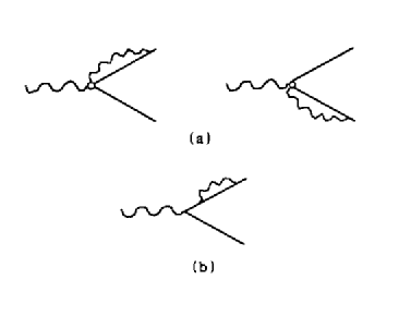
Figure 20: Leading collinear reduced diagrams at one loop: (a) covariant gauge, (b) physical gauge.

By doing the $k^{-}$ integral by contour integration, we easily find that in Feynman gauge the contribution of momenta close to the singularity where $k$ is proportional to $p$ is given by

$$V_{\mu}(p,p^{\prime})\approx\frac{i}{(2\pi)^{3}}\int_{-p^{+}}^{0}\frac{{\rm d}k^{+}}{k^{+}}{\bar{v}}(p^{\prime})\gamma_{\mu}u(p)\ g_{-+}\ (1+k^{+}/p^{+})\frac{{\rm d}^{2}{k_{\perp}}}{{k_{\perp}}^{2}},$$ (141)

and similarly in the second region. We have exhibited explicitly the numerator of the gluon propagator. For fixed $k^{+}=-xp^{+}$, the ${k_{\perp}}$ integral diverges, and is leading power, that is, independent of $Q$. This is the collinear divergence. (There is an additional infrared divergence as $k^{+}$ vanishes; this region we have already discussed. This result for the $Q$ dependence is known as a “Sudakov” double logarithm; it is associated with the overlap of collinear and infrared divergences.)

These regions, summarized by the reduced graphs of Fig. 20(a) in which two collinear lines attach to a hard subdiagram, would not be leading in ${(\phi^{3})}_{6}$, because of the lack of the numerator factor. Note, however, that in the numerator of the gluon propagator, the term which gives the leading behavior in the collinear region is $g_{-+}$. Since the gluon is moving, by assumption, parallel to $p^{\mu}$, which is in the plus direction, this corresponds to an unphysical polarization at the vertex adjacent to the antiquark line. Thus the collinear divergence is associated with a longitudinally polarized gluon, and we might expect it to be absent in a physical gauge — at least in this particular diagram.

To verify this, we can compute $V_{\mu}$ in an axial gauge. The leading term in Eq. (141) is then replaced by

$$V_{\mu}(p,p^{\prime}) \approx \frac{i}{(2\pi)^{3}}\int_{-p^{+}}^{0}\frac{{\rm d}k^{+}}{k^{+}}{\bar{v}}(p^{\prime})\gamma_{\mu}u(p)\ (1+k^{+}/p^{+})$$ (142)

$$\times\int\frac{{\rm d}^{2}{k_{\perp}}}{{k_{\perp}}^{2}}\left(g_{-+}-\frac{n_{-}k_{+}+k_{-}n_{+}}{n\cdot k}+\frac{k_{-}k_{+}}{(n\cdot k)^{2}}\right),$$

Using Eq. (140) (and remembering that $k_{\pm}=k^{\mp}$), we easily check that the collinear divergence in (141) is absent in (142), and that the vertex diagram therefore lacks the Sudakov double logarithm in axial gauge. Of course, since the theory is gauge invariant, the corresponding physics, and in particular the double logarithm, has to show up somewhere, and in axial gauge it occurs in the one loop fermion self energy. We leave it as a simple but instructive exercise to check that this is indeed the case. Thus, in axial gauge the reduced diagrams of Fig. 20(a) do not correspond to a collinear divergence, while that of Fig. 20(b) does. We emphasize here the fact that in the Feynman gauge the jets are one-particle irreducible, while in the axial gauge they are reducible. As we shall see below, this result generalizes to all orders. In this sense, the gauge theory in a physical gauge behaves, from the point of view of reduced diagrams for collinear lines, like ${(\phi^{3})}_{6}$.

This suggests that an axial gauge is the most appropriate one for proving factorization. However, the singularities at $n\cdot k=0$ cause a lot of trouble. In the first place they obstruct [35, 36, 37] the contour deformations that we have already seen are essential to demonstrating factorization; this is equivalent to saying that the singularities violate relativistic causality on a graph-by-graph basis. Furthermore, the singularities have to be defined by some kind of principal value prescription, and it is difficult to ensure that the products of these singularities that occur in higher order graphs can be defined properly [38].

8.6 Power counting for gauge theories

As in the scalar theory, we must use power counting to identify those pinch surfaces which actually give leading regions. Again, this approach is discussed in detail in Ref. [24]. Here, we once again quote the general result. Assuming the eikonal approximation, for any leading region with reduced diagram $R$, we compute the infrared degree of divergence, $\omega(R)$, analogous to Eq. (122),

$$\omega(R)=4S+2C-2I_{S}-I_{C}+N_{2}+\frac{1}{2}N_{3}+F.$$ (143)

We have assumed a space-time dimension 4. As in (122), $S,\ I_{S},\ C$, and $I_{C}$ are, respectively the numbers of soft loops and lines, and collinear loops and lines in $R$ at the associated pinch surface. $N_{2}$ is the number of two-point functions in $R$, while $N_{3}$ the number of three-point functions all of whose external lines are in the same jet. $F$ is derived from the numerator factors where soft lines connect to collinear lines. It is positive except when all soft lines connecting to collinear lines are gluons. The suppression terms, $\frac{1}{2}N_{3}$ and $F$, are the only differences from Eq. (122).

We note that the $N_{3}$ term is present diagram-by-diagram in physical gauges [6], but that in Feynman gauge the computation holds in general only when gauge invariant sets of diagrams are combined for the hard scattering subdiagrams. In fact, in covariant gauges, individual diagrams may be much more divergent in the presence of infrared and collinear interactions than is the cross section, and may even grow with energy [39]. This is a consequence of the well-known fact that unitarity bounds on energy growth are only a property of gauge invariant sets of diagrams.

8.7 General leading regions

The general leading regions for $e^{+}e^{-}$-annihilation processes, for deeply inelastic scattering and for hard inclusive hadron-hadron scattering are quite analogous to those for the ${(\phi^{3})}_{6}$ theory. The basic difference is that lines which participate in infrared logarithms must be added to the corresponding reduced diagrams.

Fig. 21(a) shows a general leading region for a single particle inclusive cross section in $e^{+}e^{-}$ annihilation for a physical gauge, and Fig. 21(b) for a covariant gauge.

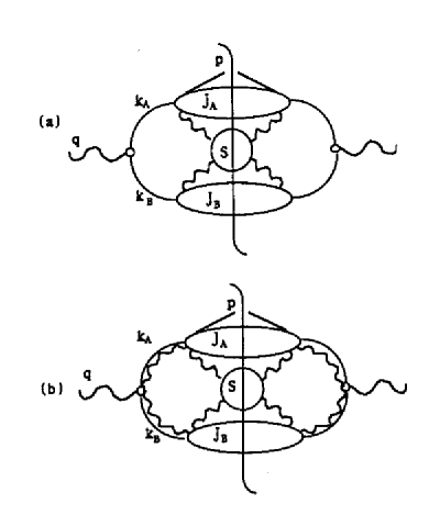
Figure 21: Typical leading regions for annihilation processes. (a) physical gauge. (b) covariant gauge. The most general leading region has the possibility of extra jets beyond the two shown here.

Compared to the leading regions for ${(\phi^{3})}_{6}$, summarized in Fig. 14, which include only jets of collinear lines and hard subdiagrams, to get Fig. 21(a) we simply add a “soft” subdiagram, consisting of lines whose momenta vanish at the pinch singular surface in question. The soft subdiagram contains in general both soft gluon lines and soft quark loops (as well as ghost loops in covariant gauges); its external lines, however, are always gluons. These external gluons always attach to (energetic) lines and not to the hard subdiagrams. The lines attaching jet subdiagrams to the hard subdiagrams may be either gluons or fermions, but at leading power only a single line from each jet enters a given hard subdiagram, just as in ${(\phi^{3})}_{6}$. The physical picture is also the same as in ${(\phi^{3})}_{6}$; several hard particles recede from a hard scattering at the speed of light, forming jets by their self-interactions. These particles can never interact with each other except by transfer of soft momenta $|k^{\mu}|\ll Q$. The presence of vector particles in the gauge theory, however, does give leading power contributions from the exchange of soft particles. Since $k^{\mu}/Q\approx 0$ for each of these particles, they do not affect those of the Landau equations, (112) and (113), which involve only the jet subdiagrams. Of course, it should be kept in mind that the soft lines have zero momentum only at the exact pinch singular surface. Feynman integrals get contributions from an entire region near this surface where the soft momenta are much smaller than a typical energy of a jet, but may approach a nonzero fraction of that energy.

For a covariant gauge, the leading regions are essentially the same, except that, just as in the one-loop case, arbitrary numbers of longitudinally polarized gluons may attach the jet to the hard part, as shown in Fig. 21(b).

Figures 22(a) and 22(b) show general leading regions for inclusive deeply inelastic scattering, and the Drell-Yan cross sections in Feynman gauge. As with ${(\phi^{3})}_{6}$, the sum over final states eliminates pinch singularities involving final state jets. The remaining on-shell lines make up the jets associated with the incoming particles including soft exchanges within and between the jets. In covariant gauges, longitudinally polarized gluons may connect the jets to the hard part.

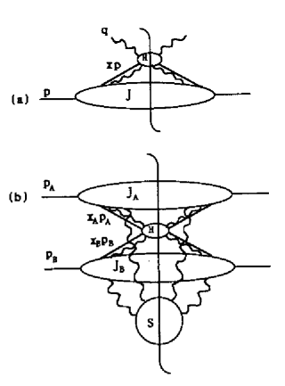
Figure 22: Leading regions in Feynman gauge for (a) inclusive deeply inelastic scattering and (b) Drell-Yan cross sections.

9 Factorization Proofs in Gauge Theories

We are now ready to discuss the extension of factorization theorems to gauge theories, for the basic cross sections discussed above: deeply inelastic scattering, single particle inclusive annihilation and Drell-Yan production. Each of these will require new reasoning relative to the scalar case.

Compared to the proof in Sect. 6 for ${(\phi^{3})}_{6}$, our treatment of factorization in gauge theories will be much more modest. Rather than derive closed expressions for the factorized forms in terms of explicit subtraction operators, we will deal with the cross sections on a region-by-region basis. We will show that an arbitrary leading region either contributes to the factorized form of the cross section, or cancels to leading power when gauge invariant sets of diagrams are combined.

9.1 Deeply inelastic scattering and collinear factorization

We start with the deeply inelastic scattering cross section, $h(p)+\gamma^{*}(q)\rightarrow X$, with $p^{\mu}(q^{\mu})$ being the momentum of the incoming hadron $h$ (virtual photon $\gamma^{*}$). Here, as we shall see, the question of factorization reduces to a treatment of collinear singularities associated with unphysically polarized gluons.

Fig. 22(a) illustrates the leading regions in a gauge theory for diagrams that contribute to the structure function tensor $W^{\mu\nu}(q,p)$. There is a single jet $J$, in the direction of the incoming particle, and a single hard subdiagram $H^{\mu\nu}$, containing the hard scattering. Divergences associated with final state interactions cancel because of unitarity in the sum over different final state cuts of the same Feynman graph. Thus we have not included regions in which soft gluons from the jet $J$ interact with the outgoing particles in the hard part $H$, even though such regions can give leading contributions to individual cut graphs.

In Feynman gauge, the hard subdiagram is connected to the single jet by more than one collinear line. This makes the transition to the convolution form of Eq. (2) more complex than in the scalar case.

In physical gauges, the reduced diagram corresponding to an arbitrary leading region has the same form as for the scalar theory, Fig. 9. This simplification is the reason that most of the original arguments for factorization were given in physical gauges [6], where essentially the same procedure can be used as in Sect. 6. However, it is important to show how the proof may be carried out in the covariant gauges, for two reasons. First, as mentioned above, there are difficulties associated with the unphysical singularities encountered in physical gauges, which have not been fully understood yet [38]. Although these are presumably of a technical nature, and not associated with the content of factorization, it is surely desirable not to be completely dependent on this presumption. Second, physical gauges, because of their noncovariance, are ill-suited to proofs of factorization in the crucial case of hadron-hadron scattering. So, in the interests of generality, we shall discuss deeply inelastic scattering in the Feynman gauge. These issues were not treated in Ref. [6].

Let us consider a typical cut Feynman diagram $G^{(C)}$, where $C$ labels the cut, in the neighborhood of a leading region $L$. $L$ is specified completely once we specify how the graph $G$ is to be decomposed into the subgraphs $J$ and $H$. We shall write the contribution from region $L$ to $G^{(C)}$ as $G^{(L,C)}$.

Referring to Fig. 22(a), we see that our problem is to organize the set of longitudinally polarized lines which attach the jets to the hard parts. Suppose a set of $n$ gluons of momentum $l_{i}^{\alpha_{i}}$ attaches to the hard part $H$ to the left of the cut, along with a physically polarized parton of momentum $k^{\mu}-\sum_{i}l_{i}^{\mu}$. Similarly, suppose a set of $n^{\prime}$ longitudinally polarized gluons ${l^{\prime}}_{j}^{\beta_{j}}$ attaches to $H$ on the right of the cut, along with a physically polarized parton of momentum $k^{\mu}-\sum_{j}{l^{\prime}}_{j}^{\mu}$. Each momentum $l^{\mu}_{i}$ is parallel to the external momentum $p^{\mu}$ and flows into the hard part. Each ${l^{\prime}}^{\mu}_{j}$ is also parallel to $p^{\mu}$, but flows out. We sum over all cuts of the original graph $G$ consistent with this leading region, with fixed $n$ and $n^{\prime}$. We can now represent the sum over these allowed cuts $C$ of $G^{(L,C)}$ as

$${\cal G}^{(L)}(\mu){}={} \sum_{C}\ G^{(L,C)}$$

$${}={} \int\frac{{\rm d}^{4}k}{(2\pi)^{4}}\ \prod_{i}\int\frac{{\rm d}^{4}l_{i}}{(2\pi)^{4}}\prod_{j}\int\frac{{\rm d}^{4}{l^{\prime}}_{j}}{(2\pi)^{4}}$$

$$\times\sum_{C_{H}}H^{(C_{H})}\!\!\left(q^{\nu};k^{\mu}-\Sigma l_{i}^{\mu},\{l_{i}^{\alpha_{i}}\};k^{\mu}-\Sigma{l^{\prime}}_{j}^{\mu},\{{l^{\prime}}_{j}^{\beta_{j}}\}\right)^{\{\mu_{i},\nu_{j}\}}_{\eta,\eta^{\prime}}$$

$$\times\sum_{C_{J}}J^{(C_{J})}(p^{\nu};k^{\mu}-\Sigma l_{i}^{\mu},\{l_{i}^{\alpha_{i}}\};k^{\mu}-\Sigma{l^{\prime}}_{j}^{\mu},\{{l^{\prime}}_{j}^{\beta_{j}}\})_{\{\mu_{i},\nu_{j}\}}^{\eta,\eta^{\prime}},$$ (144)

where $\mu_{i}$ and $\nu_{j}$ are polarization indices for the $l_{i}$ and ${l^{\prime}}_{j}$, respectively, and $\eta$ and $\eta^{\prime}$ are the polarization indices associated with the physical partons attaching to the hard part on either side of the cut. Of necessity, the sum includes only those cuts which preserve $n$ and $n^{\prime}$, and we note that it breaks up into independent sums over the cuts of the hard part and of the jet.

The integrals in (144) are restricted to the neighborhood of the region $L$. We implicitly introduce a variable $\mu$, to set the scale of $L$. The integration region in (144) is set by requiring, for instance, that lines within $H$ have transverse momenta of order at least $\mu$, while those in $J$ have transverse momenta of $\mu$ or less. $\mu$ will later be identified with the renormalization scale for the parton distribution.

Because all lines in $H$ are, by construction, far off the mass shell, we replace the momenta of all its external particles by lightlike momenta in the corresponding jet direction. Then, if we keep only leading polarization components, the extra collinear gluons which attach the hard part to the jet are exactly longitudinally polarized. Corrections are suppressed by a power of $q^{2}$. To formalize this approximation, we introduce the vectors

$$v^{\mu}=g^{\mu}_{+},\ u^{\mu}=g^{\mu}_{-},$$ (145)

and define

$$u\cdot l_{i}^{\alpha}=\lambda_{i},\ u\cdot k^{\alpha}=k,\ u\cdot{l^{\prime}}_{i}^{\alpha}=\lambda^{\prime}_{i}.$$ (146)

In terms of these variables, the approximation is

$$\sum_{C_{H}}H^{(C_{H})}(q^{\nu};k^{\mu}-\Sigma l_{i}^{\mu},\{l_{i}^{\alpha_{i}}\};k^{\mu}-\Sigma{l^{\prime}}_{j}^{\mu},\{{l^{\prime}}_{j}^{\beta_{j}}\})^{\{\mu_{i},\nu_{j}\}}_{\eta,\eta^{\prime}}\\ \rightarrow{\hat{H}}(q^{\nu};(k-\Sigma\lambda_{i})v^{\mu},\{\lambda_{i}v^{\alpha_{i}}\};(k-\Sigma\lambda^{\prime}_{j})v^{\mu},\{\lambda^{\prime}_{j}v^{\beta_{j}}\})_{\eta,\eta^{\prime}}\prod_{i}u^{\mu_{i}}\ \prod_{j}u^{\nu_{j}},$$ (147)

where

$${\hat{H}}(q^{\nu};(k-\Sigma\lambda_{i})v^{\mu},\{\lambda_{i}v^{\alpha_{i}}\};(k-\Sigma\lambda^{\prime}_{j})v^{\mu},\{\lambda^{\prime}_{j}v^{\beta_{j}}\})_{\eta,\eta^{\prime}}\\ \begin{aligned} \equiv&\sum_{C_{H}}H^{(C_{H})}(q^{\nu};kv^{\mu}-\Sigma\lambda_{i}v^{\mu},\{\lambda_{i}v^{\alpha_{i}}\};kv^{\mu}-\Sigma\lambda^{\prime}_{j}v^{\mu},\{\lambda^{\prime}_{j}v^{\beta_{j}}\})_{\eta,\eta^{\prime}}^{\{\gamma_{i},\delta_{j}\}}\\ &\times\prod_{i^{\prime}}v_{\gamma_{i}}\ \prod_{j^{\prime}}v_{\delta_{j}}.\end{aligned}$$ (148)

This replacement is analogous to the operator $P$ introduced for the scalar theory in Sect. 6.

We will now show that the unphysical polarizations of the extra gluons can be used to factor them from the hard part. The hard part will become a function of only the $total$ longitudinal momentum flowing between it and the jet, as is appropriate for a factorized form, while the longitudinally polarized gluons will couple to an eikonal line, which we associate with the jets.

Let us show this result first for the diagram on the left-hand side of Fig. 23(a), with a single longitudinally polarized gluon of momentum $l^{\mu}$, which attaches to the hard part along with the physically polarized parton of momentum $k^{\mu}-l^{\mu}$. (We shall refer to particles by their momentum labels.) If we apply the Ward identity, Eq. (131) to this set of diagrams, we find the result on the right hand side of Fig. 23(a). The left-hand side of Fig. 23(a) would vanish, except that the diagram on the right-hand side, in which the gluon $l^{\mu}$ is attached to the physical parton, is not included in $H$ by construction. But now consider the identity shown in Fig. 23(b). Here we consider a diagram in which the unphysical line ends in an eikonal line, while $H$ has a single (physically polarized) external line from $J$, which carries the total jet momentum $k$. The right hand side of Figs. 23(a) and 23(b) are the same, and we derive the identity of Fig. 23(c), in which the longitudinally polarized gluon has been factored onto an eikonal line moving in the opposite direction from the $A$-jet.

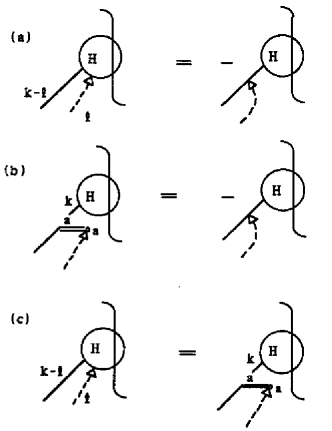
Figure 23: Ward identities for a single gluon. Group sums follow repeated indices. (a) Identity for hard part; (b) Eikonal identity; (c) Factorization of the gluon.

To be careful, we should note that in each individual cut diagram of Fig. 23, the intermediate states are not physical states, but rather states including on shell gluons with unphysical polarizations and ghosts. Once graphs for a given cut are summed over, however, we may replace the unphysical states by physical ones [31]. So we may, without loss of generality, treat the matrix elements as though they were between physical states.

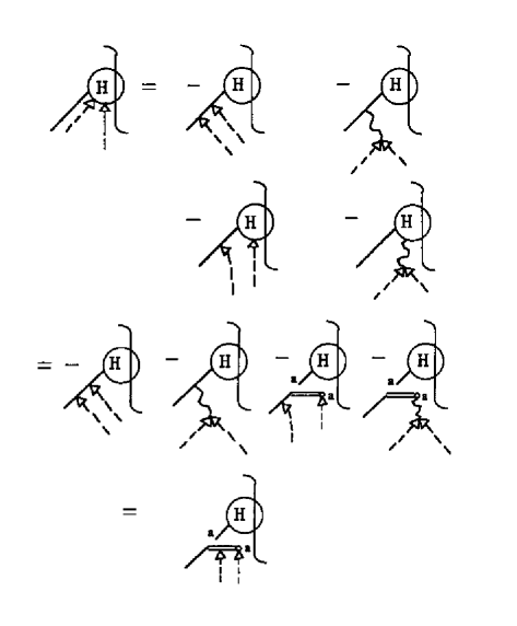
Figure 24: Application of Ward identities to two collinear gluons.

The extension of this reasoning to two gluons is straightforward. We use the identity of Fig. 24, analogous to Fig. 23. On the right hand side of the first equality in Fig. 24 we have two diagrams in which only the physical parton attaches to the hard part, and also two diagrams in which one gluon is still attached to the hard part. (Diagrams in which the two gluon lines are interchanged are not indicated explicitly in the figure.) In a covariant gauge, Lorentz invariance requires that the gluon entering the hard part in diagram $4$ also be longitudinally polarized (it has no other vectors on which to depend). Thus we can apply the result of Fig. 23 for the single gluon entering the hard part in diagrams $3$ and $4$. The result is shown in the second and third equalities in Fig. 24. This inductive approach can clearly be extended to arbitrary order, and we derive Fig. 25 for a general leading region.

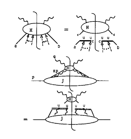
Figure 25: Factorization of collinear gluons.

This gives the overall replacement

$${\hat{H}}(q^{\nu};(k-\Sigma\lambda_{i})v^{\mu},\{\lambda_{i}v^{\alpha_{i}}\};(k-\Sigma\lambda^{\prime}_{j})v^{\mu},\{\lambda^{\prime}_{j}v^{\beta_{j}}\})_{\eta,\eta^{\prime}}\prod_{i}u^{\mu_{i}}\ \prod_{j}u^{\nu_{j}}$$

$$\hskip 56.9055pt\times J^{(C_{J})}(p^{\nu};k^{\mu}-\Sigma l_{i}^{\mu},\{l_{i}^{\alpha_{i}}\};k^{\mu}-\Sigma{l^{\prime}}_{j}^{\mu},\{{l^{\prime}}_{j}^{\beta_{j}}\})_{\{\mu_{i},\nu_{j}\}}^{\eta,\eta^{\prime}}$$

$$\rightarrow{\tilde{H}}(q^{\nu},kv^{\mu})_{\eta,\eta^{\prime}}\ {\cal E}(u,\{\lambda_{i}\})^{\{\mu_{i}\}}{{\cal E}^{*}}(u,\{\lambda^{\prime}_{j}\})^{\{\nu_{j}\}}$$

$$\hskip 56.9055pt\times J^{(C_{J})}(p^{\nu};k^{\mu}-\Sigma l_{i}^{\mu},\{l_{i}^{\alpha_{i}}\};k^{\mu}-\Sigma{l^{\prime}}_{j}^{\mu},\{{l^{\prime}}_{j}^{\beta_{j}}\})_{\{\mu_{i},\nu_{j}\}}^{\eta,\eta^{\prime}},$$ (149)

where ${\cal E}(u,\{\lambda_{i}\})^{\{\mu_{i}\}}$ is a lightlike eikonal line in the $u^{\mu}$ direction, coupled to $n$ gluons $l_{i}$, and similarly ${\cal E}^{*}(u,\{\lambda^{\prime}_{j}\})^{\{\nu_{j}\}}$ is an eikonal in the same direction coupled to the $n^{\prime}$ gluons ${l^{\prime}_{j}}$. It is natural to group the eikonal lines with the jet, and to define (compare Eq. (75))

$${\tilde{J}}(\xi)^{\eta,\eta^{\prime}} = \int\frac{{\rm d}^{4}k}{(2\pi)^{4}}\ \ \delta(\xi p\cdot u/k\cdot u-1)\ \prod_{i}\int\frac{{\rm d}^{4}l_{i}}{(2\pi)^{4}}\ \prod_{j}\int\frac{{\rm d}^{4}{l^{\prime}}_{j}}{(2\pi)^{4}}$$ (150)

$$\times{\cal E}(u,\{\lambda_{i}\})^{\{\mu_{i}\}}\ {{\cal E}^{*}(u,\{\lambda^{\prime}_{j}\})}^{\{\nu_{j}\}}$$

$$\times\sum_{C_{J}}J^{(C_{J})}(p^{\nu};k^{\mu}-\Sigma l_{i}^{\mu},\{l_{i}^{\alpha_{i}}\};k^{\mu}-\Sigma{l^{\prime}}_{j}^{\mu},\{{l^{\prime}}_{j}^{\beta_{j}}\})_{\{\mu_{i},\nu_{j}\}}^{\eta,\eta^{\prime}}.$$

The function $\tilde{J}$ is linked to the remaining hard part ${\tilde{H}}(q^{\nu},kv^{\mu})$ through only the variable $\xi$ and the physical polarization indices $\eta$ and $\eta^{\prime}$. Using (150) and (149) in (144), we have

$${\cal G}^{(L)}(\mu)=\int_{x}^{1}\frac{{\rm d}\xi}{\xi}\ {\tilde{H}}(q^{\nu},\xi p\cdot u\,v^{\mu})_{\eta,\eta^{\prime}}{\tilde{J}}(\xi)^{\eta,\eta^{\prime}},$$ (151)

where $x=-q^{2}/2p\cdot q$ as in Sect. 1. Thus in each leading region the cross section factorizes into an ultraviolet contribution times a contribution to the distribution of the physical parton which remains attached to the hard part. It is clear that we get every leading region for the parton distribution in this way. Note that when we sum over all leading regions, the perturbative sums for the hard part ${\tilde{H}}$ and the factorized jet ${\tilde{J}}$ are completely independent.

Equation (151) contains most of the physics of factorization for deeply inelastic scattering, but a few more steps are required to obtain the result (2). First, one argues using Lorentz invariance that for unpolarized incoming hadrons the hard part are both diagonal in the spin indices $\eta,\eta^{\prime}$. Thus we can sum over the spin of the partons leaving the jet part and average over the spin of the parton entering the hard part. This decouples the two factors in spin space. We then sum over all graphs and over the leading regions $L$ for each graph. The result is

$$W^{\mu\nu}\sim\sum_{a}\int_{x}^{1}\frac{{\rm d}\xi}{\xi}\ {\cal F}_{a/A}(\xi,\mu){\cal H}_{a}^{\mu\nu}(q^{\nu},\xi p\cdot u\,v^{\mu},\mu).$$ (152)

Here a sum over parton types $a$ is indicated, ${\cal F}$ is the jet part summed over graphs, leading regions, and spins, and ${\cal H}$ is the hard part summed over graphs and leading regions and averaged over the incoming spins. Both ${\cal F}$ and ${\cal H}$ depend on the parameter $\mu$ that sets the scale for the leading regions.

We can relate the functions ${\cal F}$ to the $\overline{\rm MS}$ parton distributions $f_{a/A}$ in the following manner. We note first that we can carry out exactly the same factorization procedure for parton distributions defined as in eqs. (43) and (44) as for the deeply inelastic scattering structure functions above. Then, in place of (152), we find

$$f_{b/A}(\eta,\mu)=\sum_{a}\int_{\eta}^{1}\frac{{\rm d}\xi}{\xi}\,{\hat{g}}_{ba}(\eta/\xi)\ {\cal F}_{a/A}(\xi,\mu),$$ (153)

where ${\hat{g}}_{ba}$ is some new hard part (a matrix in the space of parton types), while ${\cal F}_{a/A}$ is the same jet function as in (152). Here we define the scale of the leading regions to be the same as the renormalization scale in the parton distribution, and we use the same notation for both.

Using eqs. (152) and (153), we find the desired result for the structure functions,

$$W^{\mu\nu}(q^{\mu},p^{\mu})\sim\sum_{b}\int_{x}^{1}\frac{{\rm d}\eta}{\eta}\ f_{b/A}(\eta,\mu)\ H_{b}^{\mu\nu}\!\!\left(q^{\mu},\eta p^{\mu},\mu,\alpha_{s}(\mu)\right).$$ (154)

where the hard part $H^{\mu\nu}$ is defined by the relation

$$\sum_{b}\int_{x}^{\xi}\frac{{\rm d}\eta}{\eta}\ H_{b}^{\mu\nu}\!\!\left(q^{\mu},\eta p^{\mu},\mu,\alpha_{s}(\mu)\right)\ \hat{g}_{ba}(\eta/\xi)={\cal H}_{a}^{\mu\nu}(q^{\nu},\xi p\cdot u\,v^{\mu},\mu).$$ (155)

It should also be possible to demonstrate this factorization in the more careful manner outlined for the scalar theory in Sect. 6. From (151), the leading region $L$ may now be represented by Fig. 9, the canonical form for deeply inelastic scattering found in the scalar theory and in physical gauges. Since the same construction may be carried out for any leading region, one could define a subtraction procedure for gauge theories analogous to the one for scalar theories. The subtraction operator for a leading region $L$ then makes the replacement (147) for the hard part for the region.

9.2 Single-particle inclusive cross sections and the soft approximation

The leading regions for a single-particle inclusive cross section, $e^{+}+e^{-}\rightarrow A(p)+X$, were shown in Fig. 21. There is a jet subdiagram $J$ that describes the jet in which hadron A is observed. The hard subdiagram $H$ contains two short distance interactions (one on each side of the final state cut) involving highly virtual particles, from which one or more jets of interacting collinear particles emerge. Once again, there are extra longitudinally polarized gluons connecting the jet $J$ to the hard subdiagram $H$. More importantly, in contrast with deeply inelastic scattering, there is a soft subdiagram $S$ that connects $J$ to $H$. As a result, the factorization property fails on a graph-by-graph basis.

We recall that in any given cut Feynman graph for deeply inelastic scattering there could be soft partons connecting to the hard subdiagram, representing soft interactions between on-shell particles as they enter the final state. However, we argued that any leading region containing such soft interactions gives a cancelling contribution when one sums over the possible final state cuts for a given Feynman graph. Unfortunately, this rather trivial cancellation mechanism does not work for single particle inclusive production [40]. The reason is that we are observing a particle in the final state rather than summing freely over all final states. Nevertheless, our aim will be to show that any leading region with a soft subdiagram connecting $J$ to $H$ cancels. The only remaining leading regions are analogous to those already encountered in the case of deeply inelastic scattering, in Sect. 9.1, so that the proof of factorization sketched there carries over.

We consider the contribution from a leading region $L$ to a cut Feynman diagram. Each such cut diagram is decomposed into subdiagrams $J$, $H$, and $S$. We now sum over all cut graphs containing the same number of lines connecting the parts $J$, $H$, and $S$ on each side of the cut and call the result $G$. Our object is to show that, after summing in addition over where the lines go relative to the final state cut, $\sum G$ can be rewritten in a factorized form in the high energy limit.

In order to write the kinematic approximations, we pick lightlike vectors $v^{\mu}=g^{\mu}_{+}$ in the $p^{\mu}$ direction and $u^{\mu}=g^{\mu}_{-}$ in the $Q^{\mu},p^{\mu}$ plane, and define the momentum fraction $\xi$ of the outgoing hadron A by

$$u\cdot k=u\cdot p/\xi.$$ (156)

As in the case of deeply inelastic scattering, we use the longitudinal polarization of the extra collinear gluon lines which attach the $J$ to the hard part $H$. We once again approximate these lines by dominant momentum and polarization components, so that they appear as longitudinally polarized. Then, we sum over graphs representing different attachments of the collinear gluons to $H$ and use Ward identities to remove them from $H$ and attach them instead to eikonal lines ${\cal E}$ in the $u^{\mu}$ direction. They are then grouped with the jet to form, in this case, a fragmentation function $d_{A/a}(\xi)$. We thus derive a form analogous to (151), but with the extra complication of the soft lines,

$$G \sim \int\frac{{\rm d}\xi}{\xi}\prod_{l}\int\frac{{\rm d}^{4}q_{l}}{(2\pi)^{4}}\prod_{j}\int\frac{{\rm d}^{4}{\bar{q}}_{j}}{(2\pi)^{4}}\ \delta^{4}(\Sigma q_{l}^{\mu}+\Sigma{\bar{q}}_{j}^{\mu})$$ (157)

$$\times{J}\!\left(\xi,\{q_{l}^{\nu}\}\right)_{\eta\eta^{\prime}}^{\{\sigma_{l}\}}S(q_{l}^{\alpha},{\bar{q}}_{j}^{\beta})_{\{\sigma_{l},\tau_{j}\}}$$

$$\times{H}\!\left(Q^{\mu},(u\cdot p/\xi)v^{\mu},\{{\bar{q}}_{j}^{\nu}\}\right)^{\eta\eta^{\prime}\{\tau_{j}\}}.$$

Here $J$ is analogous to the function $\tilde{J}$ in Eq. (150). It includes the original jet subgraph together with eikonal lines attached to the ‘extra’ longitudinally polarized gluons that formally attached to the hard part. The indices $\eta,\eta^{\prime}$ represent the polarization of the physical parton that enters the hard part carrying momentum $k^{\mu}\sim(u\cdot p/\xi)v^{\mu}$. The extra complication compared to deeply inelastic scattering is the soft subgraph $S$, which couples to $J$ and $H$ via soft gluons as indicated in (157).

It is useful to interpret (157) in the language of Sect. 9.1. It describes the jet $A$ containing the observed hadron $A$ together with the unobserved jets that we have included in $H$. All of these jets emerge from a hard scattering and evolve independently, except for the exchange of soft partons, which are coupled to the color current of each jet. In the frame of jet $A$, for instance, all the charges within the other jets are moving at nearly the speed of light. But then, according to the discussion of Sect. 9.1, the Lorentz transformed field due to these jets should be nearly gauge equivalent to zero. Of course, since jet $A$ arises from a quark or gluon, it is not gauge invariant. We might expect, however, that we can exhibit the gauge nature of this interaction. To do so, we need a generalization of the eikonal approximation which we applied in Sect. 8.4 to single parton lines coupled to soft radiation.

The relevant generalization of the eikonal approximation has been termed the “soft approximation” [36, 37, 40, 41]. For the $A$-jet,it consists of making the replacement

$${J}\!\left(\xi,\{q_{l}^{\nu}\}\right)_{\eta\eta^{\prime}}^{\{\sigma_{l}\}}\rightarrow{J}\!\left(\xi,\{\hat{q}_{l}^{\nu}\}\right)_{\eta\eta^{\prime}}^{\{\alpha_{l}\}}u_{\alpha_{1}}\cdots u_{\alpha_{n}}v^{\sigma_{1}}\cdots v^{\sigma_{n}},$$ (158)

in which we define

$${\hat{q}}^{\alpha}=q\cdot v\ u^{\mu}.$$ (159)

This approximation replaces each soft gluon entering the $A$-jet by a fictitious gluon whose momentum and polarization are both in the $u$-direction. Before justifying the soft approximation, let us see what its consequences are.

Once we make the soft approximation, each cut jet diagram is a contribution to a product of matrix elements precisely of the form to which the Ward identity of Eq. (133) can be applied, with the field $\Phi(x)$ now representing the field associated with the physically polarized parton which couples to the hard part. As a result, we have at out disposal a Ward identity, which can be used to factor soft lines from the jet subdiagram, by an iterative argument very similar to the one just used to factor longitudinally polarized collinear gluons from the hard part. The details of the argument are slightly more complex because of the extra eikonal line, and we refer the interested reader to Refs. [36] and [37] for details. Here we simply quote the result, which is illustrated in Fig. 26 and may be expressed as

$${J}_{ab}\!\left(\xi,\{\hat{q}_{l}^{\nu}\}\right)_{\eta\eta^{\prime}}^{\{\alpha_{l}\}}u_{\alpha_{1}}\cdots u_{\alpha_{n}}v^{\sigma_{1}}\cdots v^{\sigma_{n}}\\ =\frac{1}{d(R)}\ {J}_{dd}\!\left(\xi\right)_{\eta\eta^{\prime}}{\cal E}(v^{\mu},{\hat{q}}^{\alpha}_{L})_{ac}^{\{\sigma(L)_{l}\}}{{\cal E}^{*}}(v^{\mu},{\hat{q}}^{\alpha}_{R})_{cb}^{\{\sigma(R)_{l}\}}$$ (160)

where ${\cal E}_{ac}(v^{\mu},{\hat{q}}^{\alpha}_{L})$ stands for the lightlike eikonal line in the $v^{\mu}$ direction, to which have been connected those soft gluons to the left of cut $C$, with momenta ${\hat{q}}^{\alpha}_{L}$ and polarization indices $\sigma(L)$. ${\cal E}^{*}$ is defined similarly in terms of soft gluons to the right of the cut, with momenta ${\hat{q}}^{\alpha}_{R}$ and polarization indices $\sigma(R)$. Finally, we have made color indices $a,b,\cdots$ explicit, and $d(R)$ is the dimension of the color representation of the physical parton.

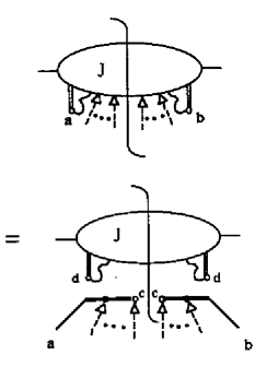
Figure 26: Factorization of soft lines from a jet.

The complete Green function may now be written in the form

$$G \sim \int\frac{{\rm d}\xi}{\xi}\frac{1}{d(R)}\ {J}_{dd}\!\left(\xi\right)_{\eta\eta^{\prime}}\prod_{l}\int\frac{{\rm d}^{4}q_{l}}{(2\pi)^{4}}\prod_{j}\int\frac{{\rm d}^{4}{\bar{q}}_{j}}{(2\pi)^{4}}\ \delta^{4}(\Sigma q_{l}^{\mu}+\Sigma{\bar{q}}_{j}^{\mu})$$ (161)

$$\times{\cal E}(v^{\mu},{\hat{q}}^{\alpha}_{L})_{ac}^{\{\sigma(L)_{l}\}}{{\cal E}^{*}}(v^{\mu},{\hat{q}}^{\alpha}_{R})_{cb}^{\{\sigma(R)_{l}\}}S(q_{l}^{\alpha},{\bar{q}}_{j}^{\beta})_{\{\sigma_{l},\tau_{j}\}}$$

$$\times{H}_{ab}\!\left(Q^{\mu},\xi u\cdot qv^{\mu},\{{\bar{q}}_{j}^{\nu}\}\right)^{\eta\eta^{\prime}\{\tau_{j}\}}.$$

Notice that the jet function has now been factored from the rest of the process. When we now perform a sum over cuts, we can sum independently over the cuts of $J$ and over the cuts of the rest of the diagram. In the rest of the diagram, we have a hard interaction producing the eikonal line ${\cal E}$ and the jets in $H$. These are coupled by final state interactions with the soft gluons in $S$. By the general reasoning of Sect. 7.6, these final state interactions cancel. Thus any leading region with soft exchanges cancels, and the factorization reasoning reverts to the arguments which apply in the scalar theory. We shall skip giving these details, and will close this subsection with a justification of the all-important soft approximation, Eq. (158).

The soft approximation consists of an approximation for the polarizations, and an approximation for soft momenta. The former may be justified by detailed power counting arguments [24], but the underlying motivation is simply that gluon polarizations proportional to $u^{\mu}$ can couple to the $A$-jet by contracting into vectors proportional to $p^{\mu}$, the momentum of the hadron A. Since $u\cdot p=p^{+}$ is a large invariant, it will dominate by a power over invariants formed from the other internal momentum components present in $J$. Note, by the way, that in Feynman gauge gluon polarizations will have nonvanishing projections onto $u^{\mu}$ only if the soft subdiagram couples to other parts of the diagram as well as $J$.

The approximation associated with the gluon momentum is more subtle. Recall that the $A$-jet is in the plus direction. We claim that one can neglect the transverse momentum of the gluon compared to its minus momentum. As we have seen in Sect. 8.4, this is nontrivial. In fact, regions where the transverse momentum is nonnegligible are leading by power counting.

Recalling the one-loop discussion of Sect. 8.4, a typical denominator from the $A$-jet on the left of the cut is of the form of

$$(\ell-q_{i})^{2}+i\epsilon\sim\ell^{2}-2\ell^{+}q_{i}^{-}+2{\ell_{\perp}}\cdot{q_{\perp}}_{i}-|{q_{\perp}}_{i}|^{2}+i\epsilon$$ (162)

with $\ell^{\mu}$ a typical line momentum in the $A$-jet. We would like to set ${q_{\perp}}_{i}$ to zero in all denominators like (162), and all we need for that is

$$|q_{i}^{-}|\gg\frac{|2{\ell_{\perp}}\cdot{q_{\perp}}_{i}-|{q_{\perp}}_{i}|^{2}|}{p^{+}}.$$ (163)

The relevant question is thus whether the $q^{-}_{i}$ momentum contours are trapped at $q^{-}_{i}=0$, at the scale of $(2{\ell_{\perp}}\cdot{q_{\perp}}_{i}-|{q_{\perp}}_{i}|^{2})/p^{+}$. Note that poles of this type can $only$ come from denominators from the $A$-jet, and not from the hard part or the soft subdiagram. Now, although every jet line through which $q^{\mu}$ flows gives a pole at a position like (162), close to the origin in the $q_{i}^{-}$ plane, all of these poles are on the same side of the real axis. To see this, consider how each soft momentum $q_{i}^{-}$ flows from the vertex where it attaches to $J$ to the parton line that attaches $J$ to $H$. In general, the $q^{-}$ pole from any jet line is in the upper half plane if $q^{-}$ flows in the opposite sense relative to the large plus momentum carried by that line. But $q^{\mu}$ may always be chosen to flow so that $q^{-}$ is directed in this sense for each jet line on which it appears. This is evident from Fig. 21. Soft gluons to the right of the cut may be treated analogously. As a result, the $q^{-}_{i}$ contours may all be deformed away from jet poles into a region where ${q_{\perp}}_{i}$ may be neglected, and the soft approximation is justified along the deformed contour. By Cauchy’s theorem, it is also justified in the original integral. Thus, the factorization program may be carried out in $e^{+}e^{-}$ annihilation.

9.3 The Drell-Yan cross section

The thorniest factorization theorems involve two hadrons in the initial state. The Drell-Yan cross section for the process

$$A(p_{A})+B(p_{B})\rightarrow\ell^{+}\ell^{-}(Q^{\mu})+X$$ (164)

is the simplest of these, and has therefore received essentially all the attention. $Q^{\mu}$ will represent the momentum of the lepton pair $\ell^{+}\ell^{-}$. The step from Drell-Yan to more complex processes, involving observed hadrons or jets in the final state is relatively straightforward, as indicated in Sect. 7.6.

Factorization for the Drell-Yan cross section has, at times, been the subject of controversy [34, 42, 43], although more recent work has, we believe, established its validity at all orders [35, 36, 37]. Nevertheless, as we shall observe below, there is plenty of room for improvement in our understanding.

The general leading region for the Drell-Yan process is shown in Fig. 22(b). After the sum over final states, all nonforward hadron jets are absorbed into the hard subdiagram $H$, in the same way as in deeply inelastic scattering. In common with the deeply inelastic scattering and one particle inclusive $e^{+}e^{-}$ annihilation processes, we can factor collinear gluons from the hard part. Once this is done, the sum of cut Feynman diagrams for the Drell-Yan cross section is very similar to Eq. (157) for $e^{+}e^{-}$ annihilation,

$$G \sim \int\frac{{\rm d}\xi_{A}}{\xi_{A}}\int\frac{{\rm d}\xi_{B}}{\xi_{B}}\prod_{l}\int\frac{{\rm d}^{4}q_{l}}{(2\pi)^{4}}\prod_{j}\int\frac{{\rm d}^{4}{\bar{q}}_{j}}{(2\pi)^{4}}\ \delta^{4}(\Sigma q_{l}^{\mu}+\Sigma{\bar{q}}_{j}^{\mu})$$ (165)

$$\times{J_{A}}\!\left(\xi_{A},\{q_{l}^{\nu}\}\right)_{\eta\eta^{\prime}}^{\{\sigma_{l}\}}{J_{B}}\!\left(\xi_{B},\{q_{l}^{\nu}\}\right)_{\eta\eta^{\prime}}^{\{\tau_{l}\}}S(q_{l}^{\alpha},{\bar{q}}_{j}^{\beta})_{\{\sigma_{l},\tau_{j}\}}$$

$$\times{H}\!\left(Q^{\mu},\xi_{A}(u\cdot p_{A})v^{\mu},\xi_{B}(v\cdot p_{B})u^{\mu}\right)^{\eta\eta^{\prime}},$$

where the lightlike vectors $v^{\mu}=g^{\mu}_{+},u^{\mu}=g^{\mu}_{-}$ have been chosen in the $p_{A}^{\mu},p_{B}^{\mu}$ directions, respectively and the parton momentum fractions are defined by $\xi_{A}=k_{A}\cdot u/p_{A}\cdot u$ and $\xi_{B}=k_{B}\cdot v/p_{B}\cdot v$. Here ${J_{A}}(\xi_{A},\{q_{l}^{\nu}\})$ and ${J_{B}}(\xi_{B},\{q_{l}^{\nu}\})$ are similar to the parton distribution function $\tilde{J}$ defined for deeply inelastic scattering in Eq. (150), except that soft gluons are still attached to them. Connections between the parton distribution and a soft subdiagram were absent in the deeply inelastic scattering cross section, because, after the sum over cuts, there was only one jet, which cannot by itself produce large invariants in numerator factors. In (165) we have a soft subdiagram as in $e^{+}e^{-}$ annihilation, but now interacting with the jets associated with the two incoming hadrons.

Our basic problem is the same as in $e^{+}e^{-}$ annihilation, to show that contributions from any leading region with a nontrivial soft subdiagram cancel in the sum over final states and gauge invariant sets of diagrams. Then the remaining leading regions of Eq. (165) are just of a form similar to Eq. (144), and the arguments for factorization may be given as above for deeply inelastic scattering, eqs. (152) to (155). Naturally, we would like to proceed by analogy to $e^{+}e^{-}$ annihilation. Thus, we would like to apply the soft approximation to the jets, and factor the soft gluons from them. The jets would then contribute to parton distributions as in Eq. (153), and, once the remaining soft contributions cancel, we would derive the desired factorized form, Eq. (11).

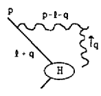
Figure 27: Example illustrating obstacles to the soft approximation.

The main obstacle to this program is shown in Fig. 27, which illustrates a typical low-order example. It shows a single soft gluon, $q^{\mu}$, attached to the A-jet. The soft momentum flows through two lines in the $A$-jet, an “active” jet line $\ell+q$ that carries positive plus-momentum into the hard part, and a “spectator” line $p-\ell-q$ that carries positive plus momentum into the final state. We saw in $e^{+}e^{-}$ annihilation that the criterion for the applicability of the soft approximation for $q^{\mu}$ is given by $|q^{-}\ell^{+}|\gg|{q_{\perp}}\cdot(2{{\ell_{\perp}}}+{{q_{\perp}}})|$, where $\ell^{\mu}$ is any line in the jet along which $q^{\mu}$ may flow. But this condition may be satisfied along the entire $q^{-}$ contour only if the contour is not pinched by poles on opposite sides of the real line. In $e^{+}e^{-}$ annihilation they are not, but in Drell-Yan they are. This is illustrated by our example, since the poles in the $q^{-}$ plane due to the jet propagators are approximately at

$$q^{-} = \frac{(p-\ell)^{2}+2({p_{\perp}}-{\ell_{\perp}})\cdot{q_{\perp}}-|{q_{\perp}}|^{2}+i\epsilon}{2(p-\ell)^{+}},$$

$$q^{-} = \frac{-\ell^{2}+2{\ell_{\perp}}\cdot{q_{\perp}}+|{q_{\perp}}|^{2}-i\epsilon}{2\ell^{+}},$$ (166)

which are on opposite sides of the contour, both at a distance of order $2{\ell_{\perp}}\cdot{q_{\perp}}/p^{+}$ from the origin. Thus, in the Feynman integral associated with Fig. 27, the $q^{-}$ contour is forced to go through a region in which the soft approximation fails, and we are unable to apply immediately the reasoning introduced for $e^{+}e^{-}$ annihilation.

The resolution of this problem is rather technical, and may be found in Ref. [37]. It may be understood most simply as a result of the Lorentz contraction of the colliding gluon fields, as in Sect. 8.1. In addition, we can give an intuitive picture here, based on semi-classical considerations in the center of mass frame. We consider the A-jet to be passing through a soft color field produced by the B-jet. Consider first the very softest part of the color field, with a spatial extent $\sim(1\ {\rm fm})\ [p_{A}^{+}/(1\ \,{\rm GeV})]$. The self-interactions of the partons in the A-jet are time dilated, but this field extends so far in space that it interacts with the partons on the same time scale as that of their self-interactions. However, on this distance scale, the soft gluons cannot resolve the hadron jet into individual partons. Thus the jet appears as a color singlet until the time of the hard interaction, at which time it acquires color because one parton is annihilated. The result is that the only interactions of the very soft color field occur long after the hard scattering event, and such interactions cancel because of unitarity. Consider now the part of the color field of smaller spatial extent, say 1 fm. The point is that the interactions of this color field with the spectator partons in the A-jet don’t really matter. The reason is that the self-interactions of the partons in the A-jet are time dilated, so that the spectator partons do not interact with the active parton on the 1 fm time scale in which they interact with the color field. Since the spectator partons are not observed, unitarity implies that their interactions with the color field will not affect the cross section. As a technical trick, we could as well replace all of the spectator partons with an equivalent color charge located at ${x_{\perp}}=0$, right on top of the active quark. Then the color field sees a net color singlet in the initial state and a net colored charge in the final state. Again, the only interactions of the color field occur long after the hard scattering event, and such interactions cancel because of unitarity.

Finally, note that the arguments given above are asymmetric between the two incoming jets. This is natural, because it is only necessary that one of the two incoming particles move at the speed of light for our arguments to apply. Indeed, factorization should hold in the (hypothetical) scattering of a truly lightlike particle with a massive particle at any center of mass energy. We should note that explicit two-loop calculations which show that infrared divergences cancel at leading power (although not at higher twist), have been carried out for the most part with one massive and one massless (eikonal) line [44, 45].

10 Outlook and Conclusion

In the foregoing, we have described the systematics of factorization for hard inclusive cross sections in QCD, and have discussed in some detail the nature of factorization proofs, first for $(\phi^{3})_{6}$, and then for gauge theories. Along the way, we outlined a systematic approach to perturbative processes at high energy, based on the classification of leading regions.

As we have indicated above, the proof of factorization theorems in gauge theories is by no means a closed subject. Factorization proofs for inclusive processes is the first item of a whole list of subjects in which progress has been made, but for which important work remains to be done. In the following, we briefly discuss a few other significant topics which relate closely to the methods discussed in this chapter. Of great importance are extensions of the theorems to more general situations.

10.1 Factorization Proofs

Factorization proofs in nonabelian gauge theories have reached a certain level of sophistication in Refs. [35], [36] and [37]. Comparison with the discussion for $(\phi^{3})_{6}$, however, shows that there is as yet in the literature no complete and systematic subtraction procedure in QCD of the type explained in Sect. 6, even in the case of deeply inelastic scattering. A subtraction algorithm would eliminate any lingering uncertainty associated with overlaps between leading regions. Perhaps even more importantly, such a procedure should make it possible to develop bounds on corrections to leading power factorization theorems, and to prove factorization theorems for nonleading power corrections, so-called “higher twist”. A model for this program is presumably to be found in the BPHZ formalism for deeply inelastic scattering cross sections in scalar and abelian gauge theories developed by Zimmermann [3], suitably modified to treat the extra infrared problems and gauge structure of QCD (see Sect. 6).

It should also be noted that the Monte-Carlo event generators [46] that are so widespread in analyzing data depend on generalizations of the factorization theorems; these generalizations have not yet gone significantly beyond the level of leading logarithms.

In addition, we should mention that additional factorization theorems, of different but related forms, are central to the analysis of the elastic scattering of hadrons, which decrease as powers of the energy [47].

10.2 Factorization at Higher Twist

It has been proposed [48] that generalized factorization theorems hold beyond the leading twist for a wide variety of cross sections. Most work on this possibility has been carried out for deeply inelastic scattering, where the systematics are best understood as a generalization of the operator product expansion [49, 50, 51]. In particular, it has been shown that multiparton distributions may be defined in a natural way to parameterize soft physics at higher twist [50, 52].

In hadron-hadron scattering, factorization at higher twist is complicated by the infrared structure of perturbative QCD. We have seen in Sect. 9 that leading twist factorization requires the cancellation of infrared divergences. It has been shown by explicit calculation [44, 45], however, that infrared divergences do $not$ cancel beyond a single loop in hadron-hadron scattering for QCD at higher twist. This is a sharp contrast between the nonabelian and abelian theories. At two loops, noncancelling divergences occur at the level $m^{4}/s^{2}$ in the Drell-Yan process. Refering to Sect. 8.1, this is precisely the level suggested by the classical relativistic kinematics of gauge fields. How one should interpret this lack of cancellation is not quite clear to us. The actual situation, including nonperturbative effects, may be better or worse than suggested by perturbative calculations [53]. The fact that perturbation theory respects factorization at $m^{2}/s$, however, makes it possible that factorization theorems may hold at this level, even for hadron-hadron scattering [54].

10.3 Factorization at the Boundaries of Phase Space

A rich class of perturbative predictions involve the summation of corrections near boundaries of phase space in different processes. Near some of these boundaries, notably small ${Q_{\perp}}$ and small $x$, cross sections increase greatly.

Along these lines, perhaps the most attention has been given to the Drell Yan cross section at measured transverse momentum ${\rm d}\sigma/{\rm d}Q^{2}{\rm d}^{2}Q_{\perp}$ [55, 56, 57], with ${Q_{\perp}}\ll Q$ and the related two-particle inclusive cross section for $e^{+}+e^{-}\rightarrow A+B+X$ at measured transverse momentum [41, 58, 59]. The complete leading-twist analysis of these cross sections begins with factorized forms of the type of Eq. (165), in which soft partons have been factored from jets, but not yet cancelled. At the boundary of phase space the cancellation of soft gluons outlined in Sect. 9 still occurs, but is incomplete. All infrared divergences still cancel at leading power, but finite remainders depend on the small parameter in the problem, for instance the transverse momentum in the cross sections cited above. By developing generalizations of the renormalization group equation for each of the functions in the factorized form Eq. (165) [41], it is possible to resum systematically higher order corrections to these quantities.

This general approach can be applied in a number of other physically important situations. For instance, the $\tau=Q^{2}/s\rightarrow 1$ limit in the inclusive Drell-Yan cross section is related to the normalization of the Drell-Yan cross section, the “K-factor” [60, 61, 62, 63]. It is possible to sum corrections which are singular at $\tau=1$ [13, 64]. An interesting feature of the result is that it is sensitive to high orders in perturbation theory [65] through the running coupling. Because of this, it gives a measure of the sensitivity to higher-twist effects of perturbative predictions based on factorization [64]. This sensitivity is found to be nonnegligible in some, but not all, regions of physical interest.

Another regime, which is of crucial importance for experiments at the Tevatron and SSC, is the $x\rightarrow 0$ limit in hadron-hadron scattering. The cross sections get into the range of tens of millibarns, which is enormous compared to typical cross sections at larger $x$. So far, much work has concentrated on the behavior of parton distributions at small $x$ [66, 67, 68, 69], assuming the validity of the standard factorization formulas (2), (3) and (11). From a more general point of view, factorization has been shown to hold explicitly in leading logarithms in $x$ [70]. We would like to suggest, however, that factorization theorems need a more extensive examination in this region.

In conclusion, we emphasize that essentially every calculation in perturbative QCD is based on one factorization theorem or another. In view of this, progress toward developing perturbative QCD as a quantitative system requires further understanding of the systematics of factorization.

11 Acknowledgements

This work was supported in part by the Department of Energy, and by the National Science Foundation.

References

- [1]
- [2] K. Wilson, Phys. Rev. 179 (1969) 1699.
- [3] W. Zimmermann, Comm. Math. Phys. 15 (1969) 208, and Ann. Phys. (N.Y.) 77 (1970) 536, 570.
- [4] N. Christ, B. Hasslacher and A.H. Mueller, Phys. Rev. D6 (1972) 3543.
- [5] W.A. Bardeen, A.J. Buras, D.W. Duke and T. Muta, Phys. Rev. D18 (1978) 3998.
- [6] D. Amati, R. Petronzio, and G. Veneziano, Nucl. Phys. B140 (1978) 54 and B146 (1978) 29; R.K. Ellis, H. Georgi, M. Machacek, H.D. Politzer, and G.G. Ross, Nucl. Phys. B152 (1979) 285; A.V. Efremov and A.V. Radyushkin, Teor. Mat. Fiz. 44 (1980) 17 [Eng. transl.: Theor. Math. Phys. 44 (1981) 573], Teor. Mat. Fiz. 44 (1980) 157 [Eng. transl.: Theor. Math. Phys. 44 (1981) 664], Teor. Mat. Fiz. 44 (1980) 327 [Eng. transl.: Theor. Math. Phys. 44 (1981) 774]; S. Libby and G. Sterman, Phys. Rev. D18 (1978) 3252, 4737; A.H. Mueller, Phys. Rev. D18 (1978) 3705.
- [7] R.P. Feynman, “Photon-Hadron Interactions”, (Benjamin, Reading, MA, 1972).
- [8] J.C. Collins, “Renormalization” (Cambridge University Press, Cambridge, 1984).
- [9] V.N. Gribov and L.N. Lipatov, Yad. Phys. 15 (1972) 781 [Engl. transl: Sov. J. Nucl. Phys. 46 (1972) 438]; L.N. Lipatov, Yad. Phys. 20 (1974) 181 [Engl. transl: Sov. J. Nucl. Phys. 20 (1975) 95]; G. Altarelli and G. Parisi, Nucl. Phys. B126 (1977) 298.
- [10] J.C. Collins and D.E. Soper, Nucl. Phys. B194 (1982) 445.
- [11] J. Kogut and D.E. Soper, Phys. Rev. D1 (1970) 2901; J.D. Bjorken, J. Kogut and D.E. Soper, Phys. Rev. D3 (1971) 1382.
- [12] B. Curci, W. Furmanski and R. Petronzio, Nucl. Phys. B175 (1980) 27; L. Baulieu, E.G. Floratos and C. Kounnas, Nucl. Phys. B166 (1980) 321.
- [13] G. Sterman, Nucl. Phys. B281 (1987) 310.
- [14] M. Diemoz, F. Ferroni, E. Longo and G. Martinelli, Z. Phys. C39 (1988) 21.
- [15] G. Altarelli, R.K. Ellis and G. Martinelli, Nucl. Phys. B157 (1979) 461.
- [16] N.N. Bogoliubov and O. Parasiuk, Acta Math. 97 (1957) 227; K. Hepp, Comm. Math. Phys. 2 (1966) 301.
- [17] See Ref. [8], for example.
- [18] G. Curci, W. Furmanski and R. Petronzio, Nucl. Phys. B175 (1980) 27; N. Isgur and C.H. Llewellyn-Smith, “The Applicability of Perturbative QCD to Exclusive Processes”, CERN preprint CERN-TH.5013/88.
- [19] A. Duncan and W. Furmanski, Nucl. Phys. B226 (1983) 339.
- [20] A.H. Mueller, Phys. Rev. D9 (1974) 963; C.G. Callan and M.L. Goldberger, Phys. Rev. D11 (1975) 1553.
- [21] L.D. Landau, Nucl. Phys. 13 (1959) 181.
- [22] R.J. Eden, P.V. Landshoff, D.I. Olive and J.C. Polkinghorne, “The Analytic S-matrix” (Cambridge University Press, Cambridge, 1966).
- [23] S. Coleman and R.E. Norton, Nuovo Cim. 28 (1965) 438.
- [24] G. Sterman, Phys. Rev. D17 (1978) 2773, 1789.
- [25] M. Creutz and L.-L. Wang, Phys. Rev. D10 (1974) 3749; S.-S. Shei, Phys. Rev. D11 (1975) 164; P. Menotti, Phys. Rev. D11 (1975) 2828.
- [26] T. Kinoshita, J. Math. Phys. 3 (1956) 65.
- [27] T.D. Lee and M. Nauenberg, Phys. Rev. 133 (1964) 1549.
- [28] S.J. Chang and S.K. Ma, Phys. Rev. 180 (1969) 1506.
- [29] G. Sterman and S. Weinberg, Phys. Rev. Lett. 39 (1977) 1436.
- [30] G. Itzykson and J.-B. Zuber, “Quantum Field Theory” (McGraw-Hill, New York, 1980).
- [31] G. ’t Hooft, Nucl. Phys. B33 (1971) 173.
- [32] G. ’t Hooft and M. Veltman, Nucl. Phys. B50 (1972) 318.
- [33] G. Grammer and D. Yennie, Phys. Rev. D8 (1973) 4332.
- [34] G.T. Bodwin, S. Brodsky and G.P. LePage, Phys. Rev. Lett. 47 (1981) 1799.
- [35] G. Bodwin, Phys. Rev. D31 (1985) 2616 and D34 (1986) 3932.
- [36] J.C. Collins, D.E. Soper and G. Sterman, Nucl. Phys. B261 (1985) 104.
- [37] J.C. Collins, D.E. Soper and G. Sterman, Nucl. Phys. B308 (1988) 833.
- [38] P.V. Landshoff, Phys. Lett. 169B (1986) 69, and references therein; P.J. Doust and J.C. Taylor, Phys. Lett. 197B (1987) 232.
- [39] J.M.F. Labastida and G. Sterman, Nucl. Phys. B254 (1985) 425.
- [40] J.C. Collins and G. Sterman, Nucl. Phys. B185 (1981) 172.
- [41] J.C. Collins and D.E. Soper, Nucl. Phys. B193 (1981) 381.
- [42] J.C. Collins, D.E. Soper and G. Sterman, Phys. Lett. 109B (1982) 388; J.C. Collins, D.E. Soper and G. Sterman, Phys. Lett. 134B (1984) 263.
- [43] W.W. Lindsay, D.A. Ross and C.T. Sachrajda, Nucl. Phys. B214 (1983) 61.
- [44] R. Doria, J. Frenkel and J.C. Taylor, Nucl. Phys. B168 (1980) 93; J. Frenkel, J.G.M. Gatheral and J.C. Taylor, Nucl. Phys. B233 (1984) 307. F.T. Brandt, J. Frenkel and J.C. Taylor, Nucl. Phys. B312 (1989) 589.
- [45] C. Di’Lieto, S. Gendron, I.G. Halliday and C.T. Sachrajda, Nucl. Phys. B183 (1981) 223.
- [46] B. Webber, Ann. Rev. Nucl. Part. Sci. 36 (1986) 253.
- [47] S.J. Brodsky and G.P. Lepage, this volume.
- [48] H.D. Politzer, Nucl. Phys. B172 (1980) 349.
- [49] R.L. Jaffe and M. Soldate, Phys. Lett. 105B (1981) 467.
- [50] R.K. Ellis, W. Furmanski and R. Petronzio, Nucl. Phys. B212 (1983) 29 and B207 (1982) 1.
- [51] J. Qiu, Argonne preprint, ANL-HEP-PR-88-10 (1988).
- [52] R. Jaffe, Nucl. Phys. B229 (1983) 205.
- [53] O. Nachtmann and A. Reiter, Z. Phys. C24 (1984) 283.
- [54] K. Kastella, J. Milana and G. Sterman, Phys. Rev. Lett. 62 (1989) 730.
- [55] Yu.L. Dokshitzer, D.I. Dyakonov and S.I. Troyan, Phys. Reports 58 (1980) 269.
- [56] G. Altarelli, R.K. Ellis, M. Greco and G. Martinelli, Nucl. Phys. B246 (1984) 12; G. Parisi and R. Petronzio, Nucl. Phys. B154 (1979) 427; C.T.H. Davies and W.J. Stirling, Nucl. Phys. B244 (1984) 337.
- [57] J.C. Collins, D.E. Soper and G. Sterman, Nucl. Phys. B250 (1985) 199.
- [58] C.L. Basham, L.S. Brown, S.D. Ellis and S.T. Love, Phys. Rev. D19 (1979) 2018.
- [59] J. Kodaira and L. Trentadue, Phys. Lett. 112B (1982) 66.
- [60] E.g., I.R. Kenyon, Rept. Math. Phys. 45 (1982) 1261.
- [61] G. Parisi, Phys. Lett. 90B (1980) 295; G. Curci and M. Greco, Phys. Lett. 92B (1980) 175.
- [62] W.L. van Neerven, Phys. Lett. 147B (1984) 175; T. Matsuura, S.C. van der Marck and W.L. van Neerven Phys. Lett. 211B (1988) 171.
- [63] S. Catani and L. Trentadue, “Ressumation of the QCD Perturbative Series for Hard Processes”, preprint DFF-93/3/89 (1989).
- [64] D. Appell, G. Sterman and P. Mackenzie, Nucl. Phys B309 (1988) 259.
- [65] G. ’t Hooft, in “The whys of subnuclear physics, Erice 1977”, ed. A. Zichichi (Plenum, New York, 1977); A.H. Mueller, Nucl. Phys. B250 (1985) 327.
- [66] L.N. Lipatov, this volume.
- [67] L.V. Gribov, E.M. Levin and M.G. Ryskin, Phys. Reports 100 (1983) 1.
- [68] A.H. Mueller and J.-W. Qiu, Nucl. Phys. B268 (1986) 427.
- [69] J.C. Collins, “Parton Distributions at Small ”, in Proceedings of 7th Topical Workshop on Proton-Antiproton Collider Physics, Fermilab 20-24 June 1988 (World Scientific, Singapore, 1989).
- [70] Joseph Milana, Phys. Rev. D34 (1986) 761.