RUB-TPII-05/04

The gluon content of the $\mathbf{\eta}$ and $\mathbf{\eta^{\prime}}$ mesons

N. G. Stefanis^a and S. S. Agaev^b

^aInstitut für Theoretische Physik II, Ruhr-Universität Bochum, D-44780 Bochum, Germany
^bHigh Energy Physics Lab., Baku State University, Z. Khalilov St. 23, 370148 Baku, Azerbaijan

Abstract: We analyze power-suppressed contributions to singlet pseudoscalar $\eta$ and $\eta^{\prime}$ meson transition form factors. These corrections stem from endpoint singularities and help improve the agreement between QCD theory and the experimental data, in particular, at low-momentum transfers. Using the CLEO data, we extract information on the profile of the $\eta_{1}$ and $\eta_{8}$ distribution amplitudes in the $SU(3)_{F}$ octet-singlet basis employing both the one-angle and the two-angle mixing schemes. In the former scheme, we find good agreement with the CLEO data, while in the second case, our approach requires non-asymptotic profiles for these mesons.

1 Introduction

Control over power-behaved corrections in QCD processes is crucial for the correct interpretation of high-precision experiments in which intact hadrons appear in the initial and/or final states. Prominent examples are meson-photon transition form factors, as measured by the CLEO collaboration [1] for the pion and the $\eta$ and $\eta^{\prime}$, and the recent JLab high-precision data for the pion’s electromagnetic form factor [2].

Because, theoretically, the dynamics of such exclusive processes involves the corresponding meson distribution amplitudes, one can extract crucial information about the nonperturbative partonic structure of pseudoscalar mesons. In contrast to the hard-scattering amplitude, that can be systematically computed within perturbative QCD and is specific for each process, hadron distribution amplitudes are universal quantities that encode the partonic structure of hadrons. Their computation requires the application of nonperturbative methods, like QCD sum rules with nonlocal condensates—introduced in [3, 4, 5] and recently improved in [6]—to derive a realistic pion distribution amplitude complying with the CLEO data on the pion-photon transition at the $1\sigma$ level [7]. In addition, this type of pion distribution amplitude was recently [8] used in conjunction with fixed-order [9, 10] and resummed [11, 12] Analytic Perturbation Theory to calculate the pion’s electromagnetic form factor providing very good agreement with the existing data.

Alternatively, one can use the factorization QCD approach in order to extract the shape of the pion (pseudoscalar meson) distribution amplitude directly from the data. The reliability of the latter possibility depends, however, on the way one deals with fixed-order perturbative calculations. To minimize the influence of (disregarded) higher-order contributions, while approaching the kinematic endpoint regions of the process in question (where the nonperturbative dynamics dominate), one may use Borel resummation techniques and, by this way, estimate power-behaved corrections. Indeed, this type of approach [13] was recently used to compute the pion-photon transition form factor and determine the pion distribution amplitude with results for the latter quantity close to the profiles determined with the nonlocal QCD sum rules just mentioned.

In the present exposition, we apply this type of approach (called the RC method) to extract the distribution amplitudes of the $\eta$ and $\eta^{\prime}$ mesons with particular focus being placed on their gluonic content [14]. More details of our approach can be found in [15, 16, 17, 18, 19].

2 $\eta$-$\eta^{\prime}$ mixing schemes

Physical pseudoscalar mesons $\eta$, $\eta^{\prime}$ are admixtures of $SU(3)_{\rm F}$ octet ($\eta_{8}$) and singlet ($\eta_{1}$) states:

$$\left(\begin{array}[]{c}\eta\\ \eta^{\prime}\end{array}\right)=\left(\begin{array}[]{cc}\cos{\theta_{p}}&-\sin{\theta_{p}}\\ \sin{\theta_{p}}&\cos{\theta_{p}}\\ \end{array}\right)\left(\begin{array}[]{c}\eta_{8}\\ \eta_{1}\\ \end{array}\right)\,,$$ (1)

where $\theta_{p}$ is the pseudoscalar mixing angle in the octet-singlet scheme (for a review and further references, see [20]).

On the parton level, the states $\eta_{8}$ and $\eta_{1}$ are given by

$$\left(\begin{array}[]{c}\eta_{8}\\ \eta_{1}\end{array}\right)=\left(\begin{array}[]{cc}\sin{\theta_{I}}&-\cos{\theta_{I}}\\ \cos{\theta_{I}}&\sin{\theta_{I}}\\ \end{array}\right)\left(\begin{array}[]{c}\frac{1}{\sqrt{2}}\left(u\bar{u}+d\bar{d}\right)\\ s\bar{s}\\ \end{array}\right)\,,$$ (2)

with $\theta_{I}$ being the ideal mixing angle.

Then, in turn, $\eta$ and $\eta^{\prime}$ are admixtures of $q\bar{q}$ pairs (in a quark-flavor basis) expressed via

$$\left(\begin{array}[]{c}\eta\\ \eta^{\prime}\end{array}\right)=\left(\begin{array}[]{cc}\cos{\alpha_{p}}&-\sin{\alpha_{p}}\\ \sin{\alpha_{p}}&\cos{\alpha_{p}}\\ \end{array}\right)\left(\begin{array}[]{c}\frac{1}{\sqrt{2}}\left(u\bar{u}+d\bar{d}\right)\\ s\bar{s}\\ \end{array}\right)\,,$$ (3)

where $\alpha_{p}=\theta_{p}-\theta_{I}+\pi/2$ denotes the deviation of the mixing angle from the ideal one due to the $U_{A}(1)$ anomaly—in contrast to the vector meson $\phi\,-\,\omega$ system with $\alpha_{v}\simeq 0$. Note that the flavor-singlet pseudoscalar state contains also a gluon component: “gluonium”. To accommodate the gluonic component, one has to extend the mixing scheme to a $3\times 3$ matrix with three mixing angles; i.e.,[21]

$$\left(\!\!\!\begin{array}[]{c}\eta\\ \eta^{\prime}\\ \iota\end{array}\!\!\!\right)\!\!\!\! = \!\!\!\!\left(\!\!\!\begin{array}[]{ccc}\cos{\theta_{p}}\cos{\gamma}+\sin{\theta_{p}}\cos{\phi}\sin{\gamma}&-\sin{\theta_{p}}\cos{\gamma}+\cos{\theta_{p}}\cos{\phi}\sin{\gamma}&\sin{\phi}\sin{\gamma}\\ \cos{\theta_{p}}\sin{\gamma}+\sin{\theta_{p}}\cos{\phi}&\sin{\theta_{p}}\sin{\gamma}+\cos{\theta_{p}}\cos{\phi}\cos{\gamma}&\sin{\phi}\cos{\gamma}\\ -\sin{\theta_{p}}\sin{\phi}&-\cos{\theta_{p}}\sin{\phi}&\cos{\phi}\\ \end{array}\!\!\!\right)$$ (14)

$$\times\left(\!\!\!\begin{array}[]{c}\eta_{8}\\ \eta_{1}\\ G\end{array}\!\!\!\right)\,,$$

where $\iota$ is a Glueball state and $G=|gg\rangle$ denotes gluonium. Note that $|\eta\rangle\simeq|\eta_{8}\rangle$ (because $m_{\eta}\simeq m_{8}$ due to the Gell-Mann–Okubo mass formula), so that the $|\eta_{1}\rangle$ admixture is small with practically no room for a $|G\rangle$ contribution. Hence, $\gamma=0$, and, as a result,

$$\left(\!\!\!\begin{array}[]{c}\eta\\ \eta^{\prime}\\ \iota\end{array}\!\!\!\right)=\left(\!\!\!\begin{array}[]{ccc}\cos{\theta_{p}}&-\sin{\theta_{p}}&0\\ \sin{\theta_{p}}\cos{\phi}&\cos{\theta_{p}}\cos{\phi}&\sin{\phi}\\ -\sin{\theta_{p}}\sin{\phi}&-\cos{\theta_{p}}\sin{\phi}&\cos{\phi}\\ \end{array}\!\!\!\right)\left(\!\!\!\begin{array}[]{c}\eta_{8}\\ \eta_{1}\\ G\end{array}\!\!\!\right)\,.$$ (15)

A physical state is then a superposition of the sort

$$|\psi\rangle=x|Q\rangle+y|S\rangle+z|G\rangle\,,\qquad x^{2}+y^{2}+z^{2}=1$$ (16)

with components (in the quark-flavor basis) given by

$$|Q\rangle = \frac{1}{\sqrt{2}}\left(u\bar{u}+d\bar{d}\right)$$

$$|S\rangle = |s\bar{s}\rangle$$

$$|G\rangle = |gg\rangle\,.$$ (17)

The physical states $\eta$ and $\eta^{\prime}$ are

$$|\eta\rangle=x_{\eta}|Q\rangle+y_{\eta}|S\rangle\,,\qquad|\eta^{\prime}\rangle=x_{\eta^{\prime}}|Q\rangle+y_{\eta^{\prime}}|S\rangle+z_{\eta^{\prime}}|G\rangle$$ (18)

with mixing coefficients

$$x_{\eta}^{2}+y_{\eta}^{2}=1\,,\qquad x_{\eta^{\prime}}^{2}+y_{\eta^{\prime}}^{2}+z_{\eta^{\prime}}^{2}=1$$ (19)

related to the mixing angles

$$x_{\eta}=\cos{\alpha_{p}}\,,\qquad y_{\eta}=-\sin{\alpha_{p}}$$ (20)

and

$$x_{\eta^{\prime}}=\cos{\phi}\sin{\alpha_{p}}\,,\quad y_{\eta^{\prime}}=\cos{\phi}\cos{\alpha_{p}}\,,\quad z_{\eta^{\prime}}=\sin{\phi}\,.$$ (21)

The $SU(3)_{\rm F}$ octet-singlet basis is provided by

$$|\eta_{1}\rangle \,=\, \frac{1}{\sqrt{3}}\;|u\bar{u}+d\bar{d}+s\bar{s}\rangle$$

$$|\eta_{8}\rangle \,=\, \frac{1}{\sqrt{6}}\;|u\bar{u}+d\bar{d}-2s\bar{s}\rangle\,.$$ (22)

One notes that the octet-singlet and the quark-flavor basis are equivalent, but that the parameterizations of the decay constants are different.

Let us now have a closer look to the decay constants of $M=\eta,\eta^{\prime}$ mesons. Their parameterization is defined via

$$\langle 0|J_{\mu 5}^{i}|M\rangle=if_{P}^{i}p_{\mu}\,,$$ (23)

where $J_{\mu 5}^{i}\,$ is the axial-vector current ($i=Q,S$ or $i=1,8$). In the quark-flavor basis, the decay constants follow the pattern of state mixing, i.e.,

$$f_{\eta}^{Q} = f_{Q}\cos{\alpha_{p}}\,\qquad f_{\eta}^{S}=-f_{S}\sin{\alpha_{p}}$$

$$f_{\eta^{\prime}}^{Q} = f_{Q}\sin{\alpha_{p}}\,\qquad f_{\eta^{\prime}}^{S}=f_{S}\cos{\alpha_{p}}\,.$$ (24)

In the octet-singlet basis the situation is different:

$$f_{\eta}^{8} = f_{8}\cos{\theta_{8}}\,\qquad f_{\eta}^{1}=-f_{1}\sin{\theta_{1}}$$

$$f_{\eta^{\prime}}^{8} = f_{8}\sin{\theta_{8}}\,\qquad f_{\eta^{\prime}}^{1}=f_{1}\cos{\theta_{1}}\,.$$ (25)

Note that in general, $\theta_{8}\neq\theta_{1}\neq\theta_{p}$. In the present analysis, we use the octet-singlet basis with the one-angle (standard) parameterization with

$$f_{\pi}=0.131\mbox{GeV}\,\qquad f_{1}=1.17f_{\pi}$$

$$f_{8}=1.26f_{\pi}\,\qquad\theta_{p}=-15.4^{\circ},$$ (26)

and the two-angle mixing scheme with the parameters

$$\theta_{p}=-15.4^{\circ},\;\theta_{1}=-9.2^{\circ},\;\theta_{8}=-21.2^{\circ}.$$ (27)

3 Electromagnetic $\eta\gamma$, $\eta^{\prime}\gamma$ transition form factor

In the Standard Hard-scattering Approach (HSA), the transverse momenta are neglected (collinear approximation) and the meson ($\pi$, $\eta$, $\eta^{\prime}\ldots$) consists in leading twist ($t=2$) only of valence $|q\bar{q}\rangle$ and $|gg\rangle$ Fock states. Let us summarize some important issues:

• The $\eta-\eta^{\prime}$ system shows flavor mixing due to the $SU(3)_{\rm F}$ symmetry breaking and the $U(1)_{\rm A}$ axial anomaly.

• The quark-singlet $|\eta_{1}\rangle$ and the gluonium state $|gg\rangle$ mix under evolution; both carry flavor-singlet quantum numbers.

• The gluon content of the $\eta^{\prime}$ can reach the level of $26\%$ [21].

• The meson-photon transition form factor contains a singlet and an octet part: $F_{\rm M\gamma}(Q^{2})=F_{\rm M\gamma}^{1}(Q^{2})+F_{\rm M\gamma}^{8}(Q^{2})$.

• The singlet part, $F_{\rm M\gamma}^{1}(Q^{2})$, has a quark and a gluonic component ([22]—using the standard HSA; [14]—using the endpoint-sensitive RC method). This means

  $$F_{\rm M\gamma}^{\,1g}(Q^{2})=\left(T_{\rm H}^{1}(x,Q^{2},\mu_{\rm F}^{2})\quad T_{\rm H}^{g}(x,Q^{2},\mu_{\rm F}^{2})\right)\,\otimes\,\left(\begin{array}[c]{c}\phi_{1}(x,\mu_{\rm F}^{2})\\[5.69046pt] \phi_{g}(x,\mu_{\rm F}^{2})\end{array}\right)\,,$$ (28)

  where $\otimes$ denotes integration over longitudinal momentum fractions $x$ from $0$ to $1$ and $\mu_{\rm F}$ is the factorization scale.

The transition form factor in the HSA can be expressed in terms of the convolution

$$F_{\rm M\gamma}(Q^{2})=\int_{0}^{1}dx\phi_{\rm M}(x,\mu_{\rm F}^{2})T_{\rm H}(x,Q^{2};\mu_{\rm F}^{2},\mu_{\rm R}^{2})$$ (29)

with $Q^{2}=-q^{2}>0$ and $q$ is the four-momentum of the virtual photon. Figure 1 shows an example of the Feynman diagrams contributing to $F_{\rm M\gamma}$ at NLO.

Figure 1: A sample of a Feynman diagram contributing to the (pseudoscalar) meson-photon transition form factor at NLO.

In Fig. 1, the partonic subprocess $\gamma*+\gamma\to q+\bar{q}$ is described by the hard-scattering amplitude $T_{\rm H}(x,Q^{2};\mu_{\rm F}^{2},\mu_{\rm R}^{2})$ ($\mu_{\rm R}$ being the renormalization scale), whereas the nonperturbative dynamics is contained in the universal meson distribution amplitude $\phi_{\rm M}(x,\mu_{\rm F}^{2})$. Note that $\phi_{8}$ satisfies a scalar evolution equation, analog to the $\pi$ case, while $\phi_{1}$ and $\phi_{g}$ evolve together via a $(2\!\times\!2)$-matrix evolution equation. Thus, we have [23]

$$\frac{d\phi_{8}(x,\mu_{\rm F}^{2})}{d\ln\mu_{\rm F}^{2}}=V(x,u,\alpha_{S}(\mu_{\rm F}^{2}))\,\otimes\,\phi_{8}(u,\mu_{\rm F}^{2})$$ (30)

with a LO solution given in terms of Gegenbauer polynomials $(\bar{x}\equiv 1-x)$:

$$\phi_{8}(x,\mu_{\rm F}^{2})=6x(1-x)\left[1+\!\!\!\sum_{n=2,4,\ldots}B_{n}^{\,8}(\mu_{\rm F}^{2})\;C_{n}^{\,3/2}(2x-1)\right]$$ (31)

and

$$\phi_{8}(x,\mu_{\mathrm{F}}^{2})=\phi_{8}(\bar{x},\mu_{\mathrm{F}}^{2})\,.$$

In Eq. (31), the projection coefficients $B_{n}^{8}$ encode the nonperturbative information that is not amenable to QCD perturbation theory, as we have already mentioned. On the other hand, the singlet $\phi_{1}$ and gluonium $\phi_{g}$ distribution amplitudes fulfill the matrix evolution equation

$$\frac{d}{d\ln\mu_{\rm F}^{2}}\left(\!\!\!\begin{array}[c]{c}\phi_{1}(x,\mu_{\rm F}^{2})\!\!\!\\ \phi_{g}(x,\mu_{\rm F}^{2})\!\!\!\end{array}\!\right)=\left(\!\!\!\begin{array}[]{cc}V_{qq}&V_{qg}\\[5.69046pt] V_{gq}&V_{gg}\end{array}\!\!\!\right)(x,u,\alpha_{S}(\mu_{\rm F}^{2}))\otimes\left(\!\!\!\begin{array}[c]{c}\phi_{1}(u,\mu_{\rm F}^{2})\\[5.69046pt] \phi_{g}(u,\mu_{\rm F}^{2})\end{array}\!\!\!\right)$$ (38)

with LO solutions provided by

$$\phi_{1}(x,\mu_{\rm F}^{2})\!\!\! = \!\!\!6x(1-x)\left[1+\!\!\!\sum_{n=2,4,\ldots}\!\!\!\!\!\!{\ B_{n}^{1}(\mu_{\rm F}^{2})}\>C_{n}^{3/2}(2x-1)\right]$$

$$\phi_{g}(x,\mu_{\rm F}^{2})\!\!\! = \!\!\!x(1-x)\!\!\!\sum_{n=2,4,\ldots}\!\!\!{B_{n}^{g}(\mu_{\rm F}^{2})}\>C_{n-1}^{5/2}(2x-1)\;.$$ (39)

The normalization conditions are

$$\int_{0}^{1}dx\phi_{1,8}(x,\mu_{\rm F}^{2})=1\qquad\int_{0}^{1}dx\phi_{g}(x,\mu_{\rm F}^{2})=0\,.$$ (40)

The quark component of the singlet state reads

$$\phi_{1}(x,\mu_{\rm F}^{2})=6x\overline{x}\left(1+\sum_{n=2,4..}^{\infty}\left\{B_{n}^{q}\left[\frac{\alpha_{{\rm s}}(\mu_{0}^{2})}{\alpha_{{\rm s}}(\mu_{\rm F}^{2})}\right]^{\frac{\gamma_{+}^{n}}{\beta_{0}}}+\rho_{n}^{g}B_{n}^{g}\left[\frac{\alpha_{{\rm s}}(\mu_{0}^{2})}{\alpha_{{\rm s}}(\mu_{\rm F}^{2})}\right]^{\frac{\gamma_{-}^{n}}{\beta_{0}}}\right\}C_{n}^{3/2}(x-\overline{x})\right)$$ (41)

with the symmetry condition $\phi_{1}(x,\mu_{\rm F}^{2})=\phi_{1}(\bar{x},\mu_{\rm F}^{2})$, whereas the gluon component is

$$\phi_{g}(x,\mu_{\rm F}^{2})=x\overline{x}\sum_{n=2,4..}^{\infty}\left\{\rho_{n}^{q}B_{n}^{q}\left[\frac{\alpha_{{\rm s}}(\mu_{0}^{2})}{\alpha_{{\rm s}}(\mu_{\rm F}^{2})}\right]^{\frac{\gamma_{+}^{n}}{\beta_{0}}}+B_{n}^{g}\left[\frac{\alpha_{{\rm s}}(\mu_{0}^{2})}{\alpha_{{\rm s}}(\mu_{\rm F}^{2})}\right]^{\frac{\gamma_{-}^{n}}{\beta_{0}}}\right\}C_{n-1}^{5/2}(x-\overline{x})$$ (42)

with the symmetry condition $\phi_{g}(x,\mu_{\rm F}^{2})=-\phi_{g}(\bar{x},\mu_{\rm F}^{2})$. The associated anomalous dimensions [17] are

$$\gamma_{\pm}^{n}=\frac{1}{2}\left[\gamma_{qq}^{n}+\gamma_{gg}^{n}\pm\sqrt{(\gamma_{qq}^{n}-\gamma_{gg}^{n})^{2}+4\gamma_{qg}^{n}\gamma_{gq}^{n}}\right]\,,$$ (43)

$$\rho_{n}^{q}=6\frac{\gamma_{+}^{n}-\gamma_{qq}^{n}}{\gamma_{gq}^{n}}\qquad\rho_{n}^{g}=\frac{1}{6}\frac{\gamma_{gq}^{n}}{\gamma_{-}^{n}-\gamma_{qq}^{n}}$$ (44)

with

$$\gamma_{qq}^{n} = C_{F}\left[3+\frac{2}{(n+1)(n+2)}-4\sum_{j=1}^{n+1}\frac{1}{j}\right]\,,$$

$$\gamma_{gg}^{n} = N_{c}\left[\frac{\beta_{0}}{N_{c}}+\frac{8}{(n+1)(n+2)}-4\sum_{j=1}^{n+1}\frac{1}{j}\right]\,,$$ (45)

$$\gamma_{qg}^{n}=\frac{12n_{f}}{(n+1)(n+2)},\,\,\,\,\,\gamma_{gq}^{n}=C_{F}\frac{n(n+3)}{3(n+1)(n+2)}\,.$$ (46)

The numerical values of these parameters ($n_{f}=3$) are

$$\gamma_{qq}^{2} = -\frac{50}{9},\,\,\,\,\,\gamma_{gg}^{2}=-11,\,\;\;\;\,\,\gamma_{gq}^{2}=\,\frac{10}{27},\,\,\,\,\gamma_{qg}^{2}=3$$

$$\gamma_{+}^{2} \simeq -\frac{48}{9},\,\,\,\gamma_{-}^{2}\simeq-\frac{101}{9}\,,\,\,\,\rho_{2}^{q}\simeq\frac{16}{5},\,\,\,\,\,\rho_{2}^{g}\simeq-\frac{1}{90}\,.$$ (47)

The required Gegenbauer polynomials are

$$C_{2}^{3/2}(x-\overline{x}) = \frac{3}{2}\left[5(x-\overline{x})^{2}-1\right]=6\left(1-5x\overline{x}\right)$$

$$C_{1}^{5/2}(x-\overline{x}) = 5(x-\overline{x})\,.$$ (48)

4 Hard-scattering amplitudes for the $\eta\gamma$ and $\eta^{\prime}\gamma$ transition

The form factor for the $\eta\gamma$ and $\eta^{\prime}\gamma$ transition, given by $F_{\rm M\gamma}(Q^{2})=F_{\rm M\gamma}^{1}(Q^{2})+F_{\rm M\gamma}^{8}(Q^{2})$, contains a singlet part comprising quark and gluon components:

$$Q^{2}F_{\rm M\gamma}^{1}(Q^{2}) \!\!\!=\!\!\! \int_{0}^{1}dxf_{\rm M}^{1}N_{1}\Bigl{\{}T_{\rm H,LO}^{q}(x)\phi_{1}(x,\mu_{\rm F}^{2})+\;\int_{0}^{1}dx\frac{\alpha_{{\rm s}}(\mu_{\rm R}^{2})}{4\pi}C_{\rm F}$$ (49)

$$\!\!\!\left[T_{\rm H,NLO}^{q}(x,Q^{2},\mu_{\rm F}^{2})\phi_{1}(x,\mu_{\rm F}^{2})+T_{\rm H,NLO}^{g}(x,Q^{2},\mu_{\rm F}^{2})\phi_{g}(x,\mu_{\rm F}^{2})\right]\Bigr{\}}\,.$$

The octet part contains only a quark component; it reads

$$Q^{2}F_{\rm M\gamma}^{8}(Q^{2}) = \int_{0}^{1}dxf_{\rm M}^{8}N_{8}\left[\!\!\!\!\!\!\!\!\!\!\!\!\!\!\!\!\!\phantom{\frac{\alpha_{{\rm s}}(\mu_{\rm R}^{2})}{4\pi}}T_{\rm H,LO}^{q}(x)\phi_{8}(x,\mu_{\rm F}^{2})\right.$$ (50)

$$\left.+\;\frac{\alpha_{{\rm s}}(\mu_{\rm R}^{2})}{4\pi}\,C_{\rm F}T_{\rm H,NLO}^{q}(x,Q^{2},\mu_{\rm F}^{2})\phi_{8}(x,\mu_{\rm F}^{2})\;\right]\,.$$

The expressions for the involved hard-scattering amplitudes are

$$T_{\rm H,LO}^{q}(x)=x^{-1}+\bar{x}^{-1}\,;$$ (51)

$$\!\!\!\!\!T_{\rm H,NLO}^{q}(x,Q^{2},\mu_{\rm F}^{2})=\frac{1}{x}\left[\ln{}^{2}x-\frac{x\ln x}{\overline{x}}-9\right]+\frac{1}{x}(3+2\ln x)\ln\frac{Q^{2}}{\mu_{\rm F}^{2}}+(x\leftrightarrow\overline{x})$$ (52)

$$\!\!\!\!\!T_{\rm H,NLO}^{g}(x,Q^{2},\mu_{\rm F}^{2})=\frac{x\ln{}^{2}x}{\overline{x}}+\left(6-\frac{4}{\overline{x}}\right)\ln{}x+2\frac{x\ln x}{\overline{x}}\ln\frac{Q^{2}}{\mu_{\rm F}^{2}}-(x\leftrightarrow\overline{x})$$ (53)

and the charge factors read

$$N_{1}=\frac{1}{\sqrt{3}}\left(e_{u}^{2}+e_{d}^{2}+e_{s}^{2}\right),\;\;\;\;\;N_{8}=\frac{1}{\sqrt{6}}\left(e_{u}^{2}+e_{d}^{2}-2e_{s}^{2}\right)\,.$$ (54)

5 $\eta\gamma$, $\eta^{\prime}\gamma$ transition form factor in the RC approach

Let us outline here the essentials of the endpoint-sensitive RC method.

• Solve the renormalization group equation for $\alpha_{s}(\lambda Q^{2})$ in terms of $\alpha_{s}(Q^{2})$ [24] to $\alpha_{s}^{2}(Q^{2})$ accuracy.

• Expand the hard-scattering amplitude $T(Q^{2})$ of the process as a power series in $\alpha_{s}(Q^{2})$ with factorially growing coefficients $C_{n}\sim(n-1)!$.

• Use the Borel integral technique to resum them by

  • determining first the Borel transform ${\cal B}[T]$ of this series

  • inverting then ${\cal B}[T]$ to get

    $$\!\!\!\!\!\!\!\!\!\!\![T]^{\rm resum}(Q^{2})\sim\mbox{P.V.}\int_{0}^{\infty}du\exp\left[\frac{-4\pi u}{\beta_{0}\alpha_{s}(Q^{2})}\right]{\cal B}[T](u).$$

    
    

  At this point a couple of important remarks are in order. (i) The Borel transforms contain poles on the positive $u$ axis that are exactly IR renormalon poles; hence a principal value (P.V.) prescription has to be used. (ii) A direct way to obtain the Borel resummed expressions is via the Inverse Laplace Transformation.

  Then, one finds

  $$\alpha_{s}(xQ^{2})=\frac{4\pi}{\beta_{0}}\int_{0}^{\infty}du{\rm e}^{-ut}R(u,t)x^{-u}$$ (55)

  with

  $$R(u,t)=1-\frac{2\beta_{1}}{\beta_{0}^{2}}u(1-\gamma_{\rm E}-\ln t-\ln u)\,.$$ (56)

• Endpoint singularities $x\to 1\;\bar{x}\to 1$ transform into IR renormalon (multi-)pole divergences at $u_{0}=n$ (in our case $n=1,2,3,4$) in the Borel $u$ plane.

• Removing these poles via the P.V. prescription, we obtain resummed expressions for

  $$[Q^{2}F_{{\rm M}\gamma}^{1}(Q^{2})]^{\rm resum}\;,\qquad[Q^{2}F_{{\rm M}\gamma}^{8}(Q^{2})]^{\rm resum}\,.$$

• The pole at $u_{0}=n$ of the Borel plane corresponds to power-suppressed corrections $\sim(1/Q^{2})^{n}$ contained in the scaled form factors.

Let us close this section, by commenting upon the importance of power corrections from the theoretical point of view and in comparison with the standard HSA. The latter prefers to set $\mu_{\rm R}^{2}=Q^{2}$. Then, large NLO logarithms are present. The RC method sets instead $\mu_{\rm R}^{2}=xQ^{2}$. As a result, the term $\ln(\mu_{\rm R}^{2}/xQ^{2})$ in the NLO contribution is eliminated, but the integration over $x$ gives rise to power-suppressed contributions in the endpoint regions $x\to 0,1$. Note in this context that because asymptotically both approaches have to yield the same results, one has to verify that the induced power corrections do not affect this regime, leaving the asymptotic behavior of perturbative QCD unchanged. Hence, in technical terms, one has to ensure that

$$\int_{0}^{\infty}du{\rm e}^{-ut}R(u,t)\stackrel{{\scriptstyle Q^{2}\to\infty}}{{\to}}\int_{0}^{\infty}du{\rm e}^{-ut}\,.$$

In view of the above remarks, the best (perturbative) procedure is the one that minimizes the NLO contribution while keeping power corrections under control.

The present analysis employs the following scales:

• $\mu_{\rm R}^{2}=xQ^{2}$ (renormalization scale)

• $\Lambda^{(n_{f}=4)}=0.25$ GeV

• $\mu_{0}^{2}=1$ GeV² (normalization scale)

• $\mu_{\rm F}^{2}=Q^{2}$ (factorization scale)

The estimated influence of higher-twist uncertainties is of the order of $(10-15)\%$.

6 Borel Resummed $\eta\gamma$ and $\eta^{\prime}\gamma$ transition form factors

The NLO expression for the transition form factor, calculated with the RC method [14], comprises a quark component

$$Q^{2}F_{\rm M\gamma}^{1}(Q^{2})_{1}^{\rm quark} \sim \alpha_{{\rm s}}(Q^{2}x)t(x,\mu_{\rm F}^{2})\otimes\phi_{1}(x,\mu_{\rm F}^{2})$$ (57)

$$+ \alpha_{{\rm s}}(Q^{2}\overline{x})t(\overline{x},\mu_{\rm F}^{2})\otimes\phi_{1}(x,\mu_{\rm F}^{2})$$

$$= 2\alpha_{{\rm s}}(Q^{2}x)t(x,\mu_{\rm F}^{2})\otimes\phi_{1}(x,\mu_{\rm F}^{2})$$

with

$$t(x,\mu_{\rm F}^{2})=\frac{1}{x}\left[\ln{}^{2}x-\frac{x\ln x}{\bar{x}}-9\right]+\frac{1}{x}(3+2\ln x)\ln\frac{Q^{2}}{\mu_{\rm F}^{2}}$$ (58)

and a gluon component

$$Q^{2}F_{\rm M\gamma}^{1}(Q^{2})_{1}^{\rm gluon}\sim 2\alpha_{{\rm s}}(Q^{2}x)g(x,\mu_{\rm F}^{2})\otimes\phi_{g}(x,\mu_{\rm F}^{2})$$ (59)

with

$$g(x,\mu_{\rm F}^{2})=\frac{x\ln{}^{2}x}{\overline{x}}+\left(6-\frac{4}{\overline{x}}\right)\ln x+2\ln\left(\frac{Q^{2}}{\mu_{\rm F}^{2}}\right)\frac{x\ln x}{\overline{x}}\,.$$ (60)

Summing up, we can write–in the context of the RC method–the transition form factors $Q^{2}F_{\rm M\gamma}^{1}(Q^{2})$ and $Q^{2}F_{\rm M\gamma}^{8}(Q^{2})$ as follows

$$Q^{2}F_{\rm M\gamma}^{1}(Q^{2})\!\!\! = \!\!\!f_{\rm M}^{1}N_{1}\left\{T_{{\rm H},0}^{q}(x)\otimes\phi_{1}(x,\mu_{\rm F}^{2})+\frac{C_{\rm F}}{2\pi}\left[\alpha_{{\rm s}}(Q^{2}x)t(x,\mu_{\rm F}^{2})\right.\right.$$ (61)

$$\!\!\!\!\!\otimes\!\left.\left.\phi_{1}(x,\mu_{\rm F}^{2})+\alpha_{{\rm s}}(Q^{2}x)g(x,\mu_{\rm F}^{2})\otimes\phi_{g}(x,\mu_{F}^{2})\right]\phantom{\frac{\alpha_{H}}{2\pi_{H}}}\!\!\!\!\!\!\!\!\!\!\!\!\!\right\}$$

and

$$Q^{2}F_{\rm M\gamma}^{8}(Q^{2})\!\! = \!\!f_{\rm M}^{8}N_{8}\left[T_{{\rm H},0}^{q}(x)\otimes\phi_{8}(x,\mu_{\rm F}^{2})+\frac{C_{\rm F}}{2\pi}\,\alpha_{{\rm s}}(Q^{2}x)t(x,\mu_{\rm F}^{2})\right.$$ (62)

$$\otimes\left.\phi_{8}(x,\mu_{\rm F}^{2})\phantom{\frac{\alpha_{H}}{2\pi_{H}}}\!\!\!\!\!\!\!\!\!\!\!\!\!\right]\,.$$

Now recall that the running coupling $\alpha_{s}(xQ^{2})$ in terms of $\alpha_{s}(Q^{2})$ [24] reads

$$\alpha_{\rm s}(Q^{2}x)\simeq\frac{\alpha_{\rm s}(Q^{2})}{1+\ln x/t}\left[1-\frac{\alpha_{\rm s}(Q^{2})\beta_{1}}{2\pi\beta_{0}}\frac{\ln[1+\ln x/t]}{1+\ln x/t}\right]$$

where we have used

$$t=\frac{4\pi}{\beta_{0}\alpha_{\rm s}(Q^{2})}=\ln\frac{Q^{2}}{\Lambda^{2}}\,,\quad\beta_{0}=11-\frac{2}{3}n_{f}\,,\quad\beta_{1}=51-\frac{19}{3}n_{f}\,.$$

In this way, we finally arrive at the following expressions for the resummed singlet and octet transition form factors within the RC method:

$$Q^{2}F_{\rm M\gamma}^{1}(Q^{2})\!\!\! = \!\!\!f_{\rm M}^{1}N_{1}\left\{6+A(\mu_{\rm F}^{2})+\frac{12C_{\rm F}}{\beta_{0}}\left[\!\!\!\!\!\!\!\!\!\!\!\!\phantom{\frac{\alpha_{H}}{2\pi_{H}}}\left(1+A(\mu_{\rm F}^{2})\right)\right.\right.$$ (63)

$$\times \!\!\!\left.\left.\int_{0}^{\infty}\!\!\!du{\rm e}^{-ut}R(u,t)Q_{1}(u)-5A(\mu_{\rm F}^{2})\int_{0}^{\infty}\!\!du{\rm e}^{-ut}R(u,t)Q_{2}(u)\right]\right.$$

$$+ \!\!\!\left.\frac{2C_{\rm F}}{\beta_{0}}B(\mu_{\rm F}^{2})\int_{0}^{\infty}\!\!\!du{\rm e}^{-ut}R(u,t)G(u)\right\}\;,$$

$$\!\!\!\!\!\!\!\!Q^{2}F_{\rm M\gamma}^{8}(Q^{2}) = f_{\rm M}^{8}N_{8}\left\{6+C(\mu_{\rm F}^{2})+\frac{12C_{\rm F}}{\beta_{0}}\left[\left(1+C(\mu_{\rm F}^{2})\right)\int_{0}^{\infty}du{\rm e}^{-ut}\right.\right.$$

$$\times \!\!\!\left.\left.R(u,t)Q_{1}(u)-\right.\right.\left.\left.5C(\mu_{\rm F}^{2})\int_{0}^{\infty}du{\rm e}^{-ut}R(u,t)Q_{2}(u)\right]\right\}\,.$$ (64)

In the above expressions, the following abbreviations have been used [14]:

$$R(u,t)=1-\frac{2\beta_{1}}{\beta_{0}^{2}}u(1-\gamma_{E}-\ln t-\ln u)\,,$$ (65)

$$Q_{1}(u)=\frac{2}{(1-u)^{3}}-\frac{2}{(2-u)^{3}}-\frac{2a}{(1-u)^{2}}+\frac{1+2a}{(2-u)^{2}}+3\frac{a-3}{(1-u)(2-u)}\,,$$

$$Q_{2}(u) = \frac{2}{(2-u)^{3}}-\frac{4}{(3-u)^{3}}+\frac{2}{(4-u)^{3}}-\frac{2a}{(2-u)^{2}}$$ (66)

$$\,+\, \frac{1+4a}{(3-u)^{2}}-\frac{1+2a}{(4-u)^{2}}+6\frac{a-3}{(2-u)(3-u)(4-u)}\,,$$

$$G(u)=\frac{4}{(4-u)^{3}}-\frac{2}{(3-u)^{3}}+\frac{2}{(2-u)^{2}}-2\frac{5-a}{(3-u)^{2}}+4\frac{3-a}{(4-u)^{2}}\,,$$ (67)

with $a\equiv\ln(Q^{2}/\mu_{\rm F}^{2})$ and the Gegenbauer coefficients being given by

$$A(\mu_{\rm F}^{2}) = 6B_{2}^{q}\left[\frac{\alpha_{{\rm s}}(\mu_{\rm F}^{2})}{\alpha_{{\rm s}}(\mu_{0}^{2})}\right]^{\frac{48}{81}}-\frac{B_{2}^{g}}{15}\left[\frac{\alpha_{{\rm s}}(\mu_{\rm F}^{2})}{\alpha_{{\rm s}}(\mu_{0}^{2})}\right]^{\frac{101}{81}}$$

$$B(\mu_{\rm F}^{2}) = 16B_{2}^{q}\left[\frac{\alpha_{{\rm s}}(\mu_{\rm F}^{2})}{\alpha_{{\rm s}}(\mu_{0}^{2})}\right]^{\frac{48}{81}}+5B_{2}^{g}\left[\frac{\alpha_{{\rm s}}(\mu_{\rm F}^{2})}{\alpha_{{\rm s}}(\mu_{0}^{2})}\right]^{\frac{101}{81}}$$

$$C(\mu_{\rm F}^{2}) = 6B_{2}^{q}\left[\frac{\alpha_{{\rm s}}(\mu_{\rm F}^{2})}{\alpha_{{\rm s}}(\mu_{0}^{2})}\right]^{\frac{50}{81}}\,.$$ (68)

7 Phenomenological Analysis

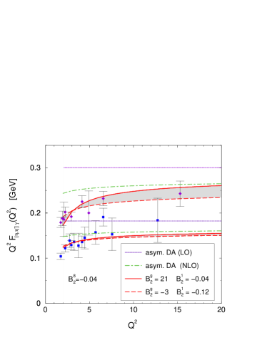
Figure 2: $\eta$ (lower curves) and $\eta^{\prime}$ (upper curves) transition form factors obtained with the standard HSA in [22]. The shaded area corresponds to the range of values $B_{2}^{8}(\mu_{0}^{2})=-0.04\pm 0.04\quad B_{2}^{1}(\mu_{0}^{2})=-0.08\pm 0.04\quad B_{2}^{g}(\mu_{0}^{2})=9\pm 12$ (see [22, 26] for further details).

In this section we perform numerical computations of the Borel resummed and rescaled by $Q^{2}$ $\eta\gamma$ and $\eta^{\prime}\gamma$ transition form factors in order to extract the $\eta$ and $\eta^{\prime}$ meson distribution amplitudes from the CLEO data. We shall also compare our theoretical predictions with those obtained with the standard HSA [22, 25], the aim being to reveal the role of power corrections at low-momentum transfer in the exclusive process under consideration.

Let us start our discussion by quoting the results obtained in [22] (see also [26]) using the standard HSA. Their main predictions are shown in Fig. 2 in comparison with the CLEO data [1].

As one sees from this figure, the agreement between the theoretical predictions and the low-momentum data is rather poor—especially when using asymptotic profiles for the $\eta$, $\eta^{\prime}$ meson distribution amplitudes. To decrease the magnitude of the form factors at low $Q^{2}$, and achieve this way a better agreement with the data, the standard HSA would call for the two-angles mixing scheme and for distribution amplitudes mainly with $B_{2}^{q}(\eta_{1}),\,B_{2}^{q}(\eta_{8})<0$. The inclusion of power-law corrections changes the low-momentum behavior of the form-factor predictions significantly, as one observes from Fig. 3. Indeed, using the standard octet-singlet mixing scheme, one can reproduce the trend of the CLEO data rather well in the whole momentum range explored—especially with a non negligible gluon contribution (the Gegenbauer coefficients are given in Fig. 3)—because the effect of power corrections is to enhance the absolute value of the NLO correction to the form factors by more than a factor of $2.5-3$. Since the contribution of the NLO term to the form factors is negative, the power corrections reduce the leading-order prediction for the form factors considerably, while at the highest $Q^{2}$ values measured by the CLEO collaboration this influence becomes more moderate.

Figure 3: Predictions for the scaled form factors as functions of $Q^{2}$ of the $\eta\gamma$ (left panel) and $\eta^{\prime}\gamma$ (right panel) electromagnetic transition. For the solid curves the designation is $B_{2}^{g}(\eta_{1})=0$. The dashed lines correspond to $B_{2}^{g}(\eta_{1})=10$; for the dash-dotted curves we use $B_{2}^{g}(\eta_{1})=15$. The data are taken from Ref. [1].

The $1\sigma$ regions in the form of shaded areas for the scaled form factors for the $\eta\gamma$ and $\eta^{\prime}\gamma$ transition in the RC method and using the octet-singlet scheme are displayed in Fig. 4. The central line corresponds to the coefficients values $B_{2}^{q}(\eta_{1})=B_{2}^{q}(\eta_{8})=0.05$;  $B_{2}^{g}(\eta_{1})=17$. A full-fledged discussion of these issues is given in [14], together with error estimates arising from varying the values of the theoretical parameters used in the analysis.

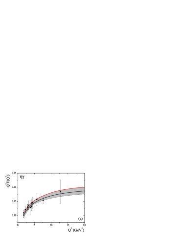
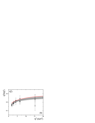
Figure 4: The $\eta\gamma$ (left) and $\eta^{\prime}\gamma$ (right) scaled transition form factors as functions of $Q^{2}$. The central solid curves are found using the values $B_{2}^{q}(\eta_{1})=B_{2}^{q}(\eta_{8})=0.05$ and $B_{2}^{g}(\eta_{1})=17$. The shaded areas demonstrate the $1\sigma$ regions for the transition form factors.

It is important to emphasize that our calculations do not exclude the usage of the two-angles mixing scheme in conjunction with the RC method. But in such a case, a considerably larger contribution of the non-asymptotic terms to the distribution amplitudes of the $\eta_{1}$ and $\eta_{8}$ states would be required. Carrying out such a computation [14], we obtained the results shown in Fig. 5. Inspection of the left panel of this figure reveals that the $\eta\gamma$ transition FF found within this scheme lies significantly lower than the data. Therefore, to improve the agreement with the experimental data, a relatively large contribution of the first Gegenbauer polynomial to the distribution amplitudes of the $\eta_{1}$ and $\eta_{8}$ states seems necessary. The Gegenbauer coefficients corresponding to the predictions shown in Fig. 5 are $B_{2}^{q}(\eta_{1})=0.15,\;B_{2}^{q}(\eta_{8})=0.15$ and $B_{2}^{g}(\eta_{1})=18$. We consider the values $B_{2}^{q}(\eta_{1})=B_{2}^{q}(\eta_{8})=0.15$ as actually determining the lower bound for the admissible set of distribution amplitudes in the context of the two-angles mixing parameterization scheme. Hence, in that scheme, we obtain

$$B_{2}^{q}(\eta_{1})=B_{2}^{q}(\eta_{8})=0.15,\;B_{2}^{g}(\eta_{1})\in[16,\,20]\,.$$ (69)

Figure 5: The $\eta\gamma$ (a) and $\eta^{\prime}\gamma$ (b) electromagnetic transition form factors vs. $Q^{2}$. The solid lines correspond to the ordinary octet-singlet mixing scheme with parameters $B_{2}^{q}(\eta_{1})=B_{2}^{q}(\eta_{8})=0.02$ and $B_{2}^{g}(\eta_{1})=18$. The broken lines are obtained within the two-angles mixing scheme. The dashed lines describe the situation with the same parameters as the solid curves. The parameters for the dash-dotted curves are $B_{2}^{q}(\eta_{1})=B_{2}^{q}(\eta_{8})=0.15,\,B_{2}^{g}(\eta_{1})=18$.

Let us close this section by summarizing the main differences between the standard HSA and the RC method: (i) Form factors in the HSA overshoot the CLEO data—especially in the low $Q^{2}$ region—even with the NLO corrections included. (ii) Values of the Gegenbauer coefficients $B_{2}^{q}(\eta_{1}),\;B_{2}^{q}(\eta_{8})>0$ increase the disagreement, while $B_{2}^{g}(\eta_{1})>0$ reduces the disagreement. Hence, a better agreement with the CLEO data would call for the two-angles mixing scheme and $B_{2}^{q}(\eta_{1})\,,B_{2}^{q}(\eta_{8})<0$. (iii) The inclusion of power corrections enhances the (negative) NLO correction to the form factors at low $Q^{2}$ by factors $2.5-3$. In order to quantify these statements, we show in Fig. 6, the numerical results for the ratio

$$R_{\rm M\gamma}(Q^{2})=\frac{[Q^{2}F_{\rm M\gamma}(Q^{2})]_{\rm NLO}^{\rm res}}{[Q^{2}F_{\rm M\gamma}(Q^{2})]_{\rm NLO}^{\rm HSA}}$$ (70)

for some selected values of the expansion coefficients. As a result, the RC method, employing the one-angle mixing scheme, is in good agreement with the CLEO data. (iv) Using instead the two-angles mixing scheme, the RC method favors non-asymptotic profiles for the distribution amplitudes of $\eta_{1}$ and $\eta_{8}$, e.g., $B_{2}^{q}(\eta_{1}),\;B_{2}^{q}(\eta_{8})\geq 0.15$ and $B_{2}^{g}(\eta_{1})\in[16,\;20]$, while the region $B_{2}^{q}(Q^{2}\simeq 2~{}{\rm GeV}^{2})<0$ seems to be incompatible with the CLEO data.

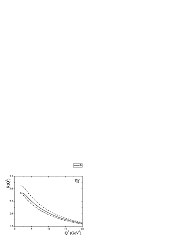
Figure 6: The ratio $R(Q^{2})$ for the $\eta\gamma$ form factor. The solid line corresponds to the input parameters $B_{2}^{q}(\eta_{1})=B_{2}^{q}(\eta_{8})=B_{2}^{g}(\eta_{1})=0$. The dash-dotted curve describes the same ratio, but for $B_{2}^{q}(\eta_{1})=B_{2}^{q}(\eta_{8})=0,\,B_{2}^{g}(\eta_{1})=14$, while the dashed one corresponds to $B_{2}^{q}(\eta_{1})=B_{2}^{q}(\eta_{8})=0.05,\,B_{2}^{g}(\eta_{1})=10$.

8 Conclusions

The renormalon-inspired RC method enables the inclusion of power corrections originating from the kinematic endpoint region ($x\to 0,1$), where nonperturbative QCD dominates and fixed-order perturbative computations of such corrections yields divergent results. We found that power-suppressed ambiguities to form factors vary between $3\%$ at high and $11\%$ at low $Q^{2}$ values. On the other hand, we have verified that the asymptotic limit of $[Q^{2}F_{{\rm M}\gamma}(Q^{2})]^{\rm resum}$ coincides, as it should, with the standard HSA result, leaving the asymptotic properties of QCD perturbation theory unchanged. The effect of power corrections at $Q^{2}\leq 5$ GeV² enhances the (negative) NLO correction by $2.5-3$ times, providing this way agreement with the trend of the CLEO data. In the standard octet-singlet scheme we found $B_{2}^{q}(\eta_{1})=B_{2}^{q}(\eta_{8})\geq 0.055\pm 0.065$,  $B_{2}^{g}(\eta_{1})=18\pm 4.5$, whereas in the two-angles mixing scheme, we found $B_{2}^{q}(\eta_{1})=B_{2}^{q}(\eta_{8})\geq 0.15$,  $B_{2}^{g}(\eta_{1})\in[16,\,20]$. The distribution amplitude of the $\eta$ and $\eta^{\prime}$ mesons, obtained in this work, can be useful in the investigation of other exclusive processes that involve $\eta$ and $\eta^{\prime}$ mesons, especially at lower momentum-transfer values, where the standard HSA is most unreliable.

Acknowledgments

One of us (N.G.S.) would like to thank the organizers of the workshop for the hospitality and the exciting atmosphere during the meeting.

References

- [1] J. Gronberg et al. (CLEO), Phys. Rev. D 57 (1998) 33.
- [2] J. Volmer et al. (The Jefferson Lab F(pi)), Phys. Rev. Lett. 86 (2001) 1713.
- [3] S. V. Mikhailov and A. V. Radyushkin, JETP Lett. 43 (1986) 712; Sov. J. Nucl. Phys. 49 (1989) 494; Phys. Rev. D 45 (1992) 1754.
- [4] A. P. Bakulev and A. V. Radyushkin, Phys. Lett. B 271 (1991) 223.
- [5] S. V. Mikhailov, Phys. Atom. Nucl. 56 (1993) 650.
- [6] A. P. Bakulev, S. V. Mikhailov and N. G. Stefanis, Phys. Lett. B 508 (2001) 279; ibid. B 590 (2004) 309(E).
- [7] A. P. Bakulev, S. V. Mikhailov and N. G. Stefanis, Phys. Rev. D 67 (2003) 074012; Phys. Lett. B 578 (2004) 91.
- [8] A. P. Bakulev, K. Passek-Kumericki, W. Schroers and N. G. Stefanis, Phys. Rev. D 70 (2004) 033014.
- [9] D. V. Shirkov and I. L. Solovtsov, Phys. Rev. Lett. 79 (1997) 1209.
- [10] D. V. Shirkov, Theor. Math. Phys. 127 (2001) 409; Eur. Phys. J. C 22 (2001) 331; D. V. Shirkov and I. L. Solovtsov, Phys. Part. Nucl. 32S1 (2001) 48.
- [11] N.G. Stefanis, W. Schroers and H.C. Kim, Phys. Lett. B 449 (1999) 299; Eur. Phys. J. C 18 (2000) 137.
- [12] A. I. Karanikas and N. G. Stefanis, Phys. Lett. B 504 (2001) 225; N. G. Stefanis, Lect. Notes Phys. 616 (2003) 153.
- [13] S. S. Agaev, Phys. Rev. D 69 (2004) 094010.
- [14] S. S. Agaev and N. G. Stefanis, Phys. Rev. D (in press) [hep-ph/0307087].
- [15] S. S. Agaev, Phys. Rev. D 64 (2001) 014007.
- [16] S. S. Agaev and A. I. Mukhtarov, Int. J. Mod. Phys. A 16 (2001) 3179.
- [17] S. S. Agaev and N. G. Stefanis, Eur. Phys. J. C 32 (2004) 507.
- [18] S. S. Agaev, Phys. Lett. B 360 (1995) 117 ibid. B 369 (1996) 379(E); [hep-ph/9611215].
- [19] S. S. Agaev, Mod. Phys. Lett. A 10 (1995) 2009; ibid. A 11 (1996) 957; ibid. A 13 (1998) 2637.
- [20] Th. Feldmann, Int. J. Mod. Phys. A 15, 159 (2000).
- [21] E. Kou, Phys. Rev. D 63 (2001) 054027.
- [22] P. Kroll and K. Passek-Kumerički, Phys. Rev. D 67 (2003) 054017.
- [23] G. P. Lepage and S. J. Brodsky, Phys. Rev. D 22 (1980) 2157; A. V. Efremov and A. V. Radyushkin, Phys. Lett. B 94 (1980) 245; Theor. Math. Phys. 42 (1980) 97 [Teor. Mat. Fiz. 42(1980) 147]; A. Duncan and A. H. Mueller, Phys. Rev. D 21 (1980) 1636.
- [24] H. Contopanagos, G. Sterman, Nucl. Phys. B 419 (1994) 77.
- [25] A. Ali and A. Ya. Parkhomenko, Eur. Phys. J. C 30 (2003) 183.
- [26] K. Passek-Kumerički, hep-ph/0311039.