$B\rightarrow J/\psi\,K^{*}$ in a Supersymmetric Right-handed Flavor Mixing Scenario

Abstract

A supersymmetric extension of the Standard Model, with maximal $\tilde{s}_{R}$-$\tilde{b}_{R}$ mixing and a new source of $CP$ violation, contain all the necessary ingredients to account for a possible anomaly in the measured $CP$ asymmetry in $B\rightarrow\phi K_{S}$ decay. In the same framework we study the decay $B\rightarrow J/\psi\,K^{*}$, paying particular attention to observables that can be extracted by performing a time dependent angular analysis, and become nonzero because of new physics effects.

I Introduction

Recent results on $B$ decay to charmonium modes, such as ${B\rightarrow J/\psi\,K_{S}(K^{*})}$, are in good agreement with the Standard Model (SM). However, for the time-dependent $CP$ asymmetry in ${B\rightarrow\phi K_{S}}$ mode, also if new results seem to show more agreement with the SM, $S_{\phi K_{S}}=0.50\pm 0.25$ (BaBar) BaBarphiKs and $S_{\phi K_{S}}=0.06\pm 0.33$ (Belle) BellephiKs , than in the past, (before ICHEP04, the world average $S_{\phi K_{S}}=0.02\pm 0.29$ Moriond ), New Physics (NP) effects could still play some role. A deviation from the SM expectation of $S_{\phi K_{S}}\cong S_{\psi K_{S}}$ would call for large $s-b$ mixing, the existence of a new source of $CP$ violation, and perhaps right-handed dynamics ChuaHouNagashima . It would be important to find confirming evidence in the future.

In anticipation of a future “super B factory” that would allow precision measurements, we study $CP$ violation in the vector-vector ${B_{d}^{0}\rightarrow J/\psi\,K^{*}}$ mode by taking into account deviations in $S_{\phi K_{S}}$. We do not expect the NP effects to show up in the branching fraction since, in contrast to $B\rightarrow\phi K_{S}$, ${B_{d}^{0}\rightarrow J/\psi K^{*}}$ decay is tree dominant. With special attention to observables related to the time dependent $CP$ asymmetry HeHou1 ; Fleischer ; LondonSinha , we focus on manifestations of NP effects. In the phenomenological analysis presented in this paper, we pay particular attention to those obserables which are expected to vanish in the SM LondonSinha .

II $B\rightarrow VV$

The ${B_{d}^{0}\rightarrow J/\psi K^{(*)}}$ decay is dominated by the tree level $\bar{b}\to c\bar{c}\bar{s}$ process, while the $CP$ phase in the corresponding penguin amplitude is highly suppressed. If NP contributions are present, it could manifest itself as direct $CP$ violation effects. This can be illustrated by the full amplitude for the decay $B\rightarrow f$,

$$A(B\rightarrow f)=ae^{i\delta^{a}}+be^{i\phi}e^{i\delta^{b}}\,,$$ (1)

where the weak phases are assumed to be zero for the first amplitude and $\phi$ for the second, and $\delta^{a,b}$ are the respectively strong phases. For the $CP$ conjugate decay $\bar{B}\rightarrow\bar{f}$ the amplitude is given by changing the sign of the weak phase $\phi$. One then obtains the direct $CP$ asymmetry

$$a_{\rm dir}^{CP} = \frac{\Gamma(B\rightarrow f)-\Gamma(\bar{B}\rightarrow\bar{f})}{\Gamma(B\rightarrow f)+\Gamma(\bar{B}\rightarrow\bar{f})}$$ (2)

$$= \frac{2ab\sin{(\delta^{a}-\delta^{b})}\sin{\phi}}{a^{2}+b^{2}+2ab\cos{(\delta^{a}-\delta^{b})}\cos{\phi}}\,,$$ (3)

which does not vanish for $\phi\neq 0$ and if the strong phase difference is also not zero. However, since the $b$ quark is rather heavy, the strong phases are expected to be small and the effect of NP in the direct $CP$ asymmetry could be washed out. It is therefore important that one can still seek for NP effects by performing a time dependent analysis and comparing $B_{d}^{0}(t)\rightarrow J/\psi K^{*}$ with $J/\psi K_{S}$. In fact, more information is contained in the time dependent angular analysis of vector-vector decays such as $B_{d}^{0}(t)\rightarrow J/\psi K^{*}$ or $\phi K^{*}$ Fleischer ; LondonSinha .

For a $B\rightarrow VV$ decay, the final state can be decomposed into three helicity amplitudes $\{A_{0},A_{\parallel},A_{\perp}\}$. $A_{0}$ corresponds to both the vector mesons being polarized along their direction of motion, while $A_{\parallel}$ and $A_{\perp}$ correspond to both polarization states being transverse to their directions of motion but parallel and orthogonal to each other, respectively Rosner . If in particular we consider the decay $B_{d}^{0}(t)\rightarrow J/\psi K^{*}$, analogous to Eq. (1) we have,

$$A_{\lambda}(B\rightarrow J/\psi K^{*}) = a_{\lambda}e^{i\delta_{\lambda}^{a}}+b_{\lambda}e^{i\phi}e^{i\delta_{\lambda}^{b}},$$ (4)

$$\bar{A}_{\lambda}(\bar{B}\rightarrow J/\psi\bar{K}^{*}) = a_{\lambda}e^{i\delta_{\lambda}^{a}}+b_{\lambda}e^{-i\phi}e^{i\delta_{\lambda}^{b}},$$ (5)

where $a_{\lambda}$ and $b_{\lambda}$ are the SM and NP amplitudes and $\delta_{\lambda}^{a,b}$ their respective strong phases, for each helicity component. The full decay amplitude becomes

$$A(B\rightarrow J/\psi K^{*}) = A_{0}g_{0}+A_{\parallel}g_{\parallel}+iA_{\perp}g_{\perp},$$ (6)

$$\bar{A}(\bar{B}\rightarrow J/\psi\bar{K}^{*}) = \bar{A}_{0}g_{0}+\bar{A}_{\parallel}g_{\parallel}-i\bar{A}_{\perp}g_{\perp},$$ (7)

with $g_{\lambda}$ the coefficients of the helicity amplitudes in the linear polarization basis Sinha . If one considers the case where $K^{*}$ and $\bar{K}^{*}$ are detected through their decay to $K_{S}\pi^{0}$ so that both $B_{d}^{0}$ and $\bar{B}_{d}^{0}$ decay to a common final state, the time dependent decay rates can be written as,

$$\Gamma(B_{d}(\bar{B}_{d})\rightarrow J/\psi\,K^{*})=e^{-\Gamma t}\sum_{\lambda\leq\sigma}\left(\Lambda_{\lambda\sigma}\pm\Sigma_{\lambda\sigma}\cos\Delta mt\mp\varrho_{\lambda\sigma}\sin\Delta mt\right)\,g_{\lambda}g_{\sigma}\,.$$ (8)

By performing an angular analysis and time dependent study of the decays $\bar{B}_{d}\rightarrow J/\psi\bar{K}^{*}$ and $B_{d}\rightarrow J/\psi K^{*}$, one can measure the observables $\Lambda_{\lambda\sigma}$, $\Sigma_{\lambda\sigma}$ and $\varrho_{\lambda\sigma}$ LondonSinha . These observables can be expressed in terms of the normalized helicity amplitudes $A_{0}$, $A_{\parallel}$ and $A_{\perp}$:

$$\Lambda_{\lambda\lambda} = \frac{{\mid A_{\lambda}\mid}^{2}+{\mid\bar{A}_{\lambda}\mid}^{2}}{2}\,,$$

$$\Sigma_{\lambda\lambda} = \frac{{\mid A_{\lambda}\mid}^{2}-{\mid\bar{A}_{\lambda}\mid}^{2}}{2}\,,$$

$$\Lambda_{\perp i} = -{\rm Im}\,(A_{\perp}A_{i}^{*}-\bar{A}_{\perp}\bar{A}_{i}^{*})\,,$$

$$\Lambda_{\parallel 0} = {\rm Re}\,(A_{\parallel}A_{0}^{*}+\bar{A}_{\parallel}\bar{A}_{0}^{*})\,,$$

$$\Sigma_{\perp i} = -{\rm Im}\,(A_{\perp}A_{i}^{*}+\bar{A}_{\perp}\bar{A}_{i}^{*})\,,$$

$$\Sigma_{\parallel 0} = {\rm Re}\,(A_{\parallel}A_{0}^{*}-\bar{A}_{\parallel}\bar{A}_{0}^{*})\,,$$

$$\varrho_{\perp i} = -{\rm Re}\left(\frac{q}{p}(A_{\perp}^{*}\bar{A}_{i}+A_{i}^{*}\bar{A}_{\perp})\right)\,,$$

$$\varrho_{\perp\perp} = -{\rm Im}\left(\frac{q}{p}A_{\perp}^{*}\bar{A_{\perp}}\right)\,,$$

$$\varrho_{\perp\perp} = {\rm Im}\left(\frac{q}{p}(A_{\parallel}^{*}\bar{A}_{0}+A_{0}^{*}\bar{A}_{\parallel})\right)\,,$$

$$\varrho_{ii} = {\rm Im}\left(\frac{q}{p}A_{i}^{*}\bar{A_{i}}\right)\,,$$ (9)

where $i=\{0,\parallel\}$, $q/p=\exp\,(-2i\phi_{\rm mix})$ with $\phi_{\rm mix}$ the weak phase in $B_{d}^{0}-\bar{B}_{d}^{0}$ mixing. From Eqs. (4) and (5) one can obtain the same observables in terms of $a_{\lambda}$, $b_{\lambda}$, $\phi$, $\delta_{\lambda}\equiv\delta_{\lambda}^{b}-\delta_{\lambda}^{a}$ and $\Delta_{i}\equiv\delta_{\perp}^{b}-\delta_{i}^{a}$ LondonSinha . In particular, $\Lambda_{\perp i}$ can be expressed as,

$$\Lambda_{\perp i}=2[a_{\perp}b_{i}\cos(\Delta_{i}-\delta_{i})-a_{i}b_{\perp}\cos(\Delta_{i}+\delta_{\perp})]\sin\phi\,.$$ (10)

The observable $\Lambda_{\perp i}$ is special, as made clear by Eq. (10), because it remains nonzero in the presence of NP effects ($\phi\neq 0$), even if the strong phase differences vanish. In contrast, direct $CP$ asymmetries $\Sigma_{\lambda\lambda}$ are washed out if the strong phase differences vanish LondonSinha .

III $B\rightarrow J/\psi\,K^{*}$

We can now proceed towards NP effects in $B\rightarrow J/\psi\,K^{*}$. We start by writing the decay amplitudes for $B\rightarrow J/\psi\,K^{*}$ using the factorization approximation, but keeping the color octet contribution HeHou2 ,

$$A_{\lambda}(B\rightarrow J/\psi K^{*}) = i\frac{G_{F}}{\sqrt{2}}V_{cb}V_{cs}^{*}f_{\psi}m_{\psi}\varepsilon_{\psi}^{\mu}(\lambda)\{a_{2}^{\rm eff}\langle K^{*}\mid\bar{s}\gamma_{\mu}(1-\gamma_{5})b\mid B\rangle$$ (11)

$$- \frac{\alpha_{s}}{2\pi}\frac{m_{b}}{q^{2}}\xi_{8}^{\prime}\langle K^{*}\mid\bar{s}i\sigma_{\mu\nu}q^{\nu}(c_{12}\gamma_{\mu}(1+\gamma_{5})+c_{12}^{\prime}(1-\gamma_{5}))b\mid B\rangle\}\,,$$

where $\lambda=\lambda_{J/\psi}=\lambda_{K^{*}}=0,\ \pm 1$ denote the helicities of the final state vector particles $J/\psi$ and $K^{*}$ in the $B^{0}$ rest frame KramerPalmer . The dominant contribution in Eq. (11) is given by the tree level term proportional to

$$a_{2}^{\rm eff}=c_{2}^{\rm eff}+\zeta\,c_{1}^{\rm eff}\,,$$ (12)

while the color dipole moment terms, with the $c_{12}$ operator coming dominantly from SM and the $c_{12}^{\prime}$ operator due exclusively to NP, give smaller corrections. In the expression for $a_{2}^{\rm eff}$ we have neglected the strong and electroweak penguin contributions. The quantity $\zeta=\frac{1}{N_{c}}+\xi_{8}$ in Eq. (12) takes the value $1/N_{c}=1/3$ in the naive factorization while deviations from $1/N_{c}$ due to non-factorizable contributions to the hadronic matrix elements are measured by the parameters $\xi_{8}$ and $\xi_{8}^{\prime}$ HeHou2 . The effective Wilson coefficients $c_{1}^{\rm eff}(m_{b})$ and $c_{2}^{\rm eff}(m_{b})$ for a $b\rightarrow s$ transition are defined in Ref. CCTY .

The way we proceed to determine the parameter $\zeta$ follows Ref. NeubertStech . We fit the branching ratios for the decays $B\rightarrow J/\psi\,K_{S}(K^{*})$ and $B\rightarrow\psi(2S)\,K^{*}$ to extract $a_{2}^{\rm eff}$. We checked explicitly that the NP effect of Ref. ChuaHouNagashima does not make significant impact on the decay rates. However, the extraction of $a_{2}^{\rm eff}$ depends on the specific model one uses for the hadronic form factors NeubertStech . In this work we use the form factors at zero momentum transfer for the $B\rightarrow V$ transitions obtained in the light-cone sum rule (LCSR) analysis BallBraun . The form factor $q^{2}$ dependence is parametrized by

$$f(q^{2})=\frac{f(0)}{1-a(q^{2}/m_{B}^{2})+b(q^{2}/m_{B}^{2})^{2}}\,,$$ (13)

where the values of the parameters $a$ and $b$ are given in Ref BallBraun . Our extracted value for $a_{2}^{\rm eff}$ is $0.20$, which using Eq. (12) and the effective Wilson coefficients of Table 1 of Ref. CCTY gives $\zeta=0.48$, or the effective number of colors $1/\zeta=2.1$. Knowing $\zeta$ one derives $\xi_{8}=0.15$ and for the value of $\xi_{8}^{\prime}$ we assume $\xi_{8}^{\prime}=\xi_{8}$ HeHou2 .

IV $B\rightarrow J/\psi K^{*}$ and NP Effects

As previously mentioned, in this work we focus on the decay $B_{d}^{0}(t)\rightarrow J/\psi\,K^{*}$ in the context of a supersymmetric model with maximal $\tilde{s}_{R}-\tilde{b}_{R}$ mixing. An approximate Abelian flavor symmetry LNS can be introduced to justify such a large mixing. In this model the right-right mass matrix $\tilde{M}^{2(sb)}_{RR}$ for the strange-beauty squark sector takes the form

$$\tilde{M}^{2(sb)}_{RR}=\left[\begin{array}[]{cc}\tilde{m}_{22}^{2}&\tilde{m}_{23}^{2}e^{-i\sigma}\\ \tilde{m}_{23}^{2}e^{i\sigma}&\tilde{m}_{33}^{2}\end{array}\right]\equiv R\left[\begin{array}[]{cc}\tilde{m}_{1}^{2}&0\\ 0&\tilde{m}_{2}^{2}\end{array}\right]R^{{\dagger}},$$ (14)

where $\tilde{m}_{ij}\sim\tilde{m}^{2}$, the squark mass scale, and

$$R=\left[\begin{array}[]{cc}\cos{\theta}&\sin{\theta}\\ -\sin{\theta}e^{i\sigma}&\cos{\theta}e^{i\sigma}\end{array}\right]\,.$$ (15)

The phase $\sigma$ is the NP weak phase which will affect the observables one can extract from an angular analysis. Because of the almost democratic structure of $\tilde{M}^{2(sb)}_{RR}$, one of the two strange-beauty squarks, $\tilde{sb}_{1}$, can be rather light, even for $\tilde{m}\sim O({\rm TeV})$. A light strange-beauty squark, together with a light gluino, can make $S_{\phi,K_{s}}$ negative for $\sigma\lesssim\pi/2$ ChuaHouNagashima .

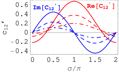
Figure 1: $c_{12}^{\prime}$ as a function of $\sigma$ for $\tilde{m}_{1}=200\ {\rm GeV}$ and $\tilde{m}=2\ {\rm TeV}$. ${\rm Re}\,(c_{12}^{\prime})$ and ${\rm Im}\,(c_{12}^{\prime})$ are plotted with solid, dash and solid-dash lines for $m_{\tilde{g}}=300,\ 500,\ 800\ {\rm GeV}$.

The main new contribution to $B_{d}^{0}(t)\rightarrow J/\psi\,K^{*}$ is given by the color dipole moment amplitude through gluino and $\tilde{sb}$ squark exchange in the loop. The analytic expressions for the Wilson coefficient $c_{12}^{\prime}$ for the color dipole moment operator $g_{s}/(8\pi^{2})m_{b}\bar{s}_{\alpha}\sigma^{\mu\nu}(1\pm g_{5})\lambda^{A}_{\alpha\beta}/2\,b_{\beta}G^{A}_{\mu\nu}$ can be found in Ref. ArhribChuaHou . The coefficient $c_{12}$ remains basically the same as $c_{12}^{\rm SM}=-0.15$. In Fig. 1 we plot the real and imaginary parts of the Wilson coefficient $c_{12}^{\prime}$ for three different values of gluino mass $m_{\tilde{g}}=300,\ 500,\ 800$ GeV . The eigenvalues of Eq. (14) are taken (with some level of tuning) as $\tilde{m}_{1}^{2}=(200\ {\rm GeV})^{2}$ and $\tilde{m}_{2}^{2}=2\tilde{m}^{2}-\tilde{m}_{1}^{2}$ with $\tilde{m}^{2}=(2\ {\rm TeV})^{2}$.

Using the parametrization for the matrix elements $\langle K^{*}\mid\bar{s}\gamma_{\mu}(1-\gamma_{5})b\mid B\rangle$ and $\langle K^{*}\mid\bar{s}i\sigma_{\mu\nu}\gamma_{\mu}(1\pm\gamma_{5})b\mid B\rangle$ given in Ref. HeHou2 the amplitudes $A_{\lambda}(B\rightarrow J/\psi K^{*})$ can be written as,

$$A_{\lambda}(B\rightarrow J/\psi K^{*}) = i\frac{G_{F}}{\sqrt{2}}V_{cb}V_{cs}^{*}f_{\psi}m_{\psi}\,\epsilon^{*}_{K^{*}\mu}(\lambda)\epsilon^{*}_{\psi\nu}(\lambda)\left\{a_{2}^{\rm eff}\left[\frac{V(m_{\psi}^{2})}{m_{B}+m_{K^{*}}}\varepsilon^{\mu\nu\alpha\beta}\,p_{K^{*}\alpha}p_{B\beta}-\frac{i}{2}(m_{B}+m_{K^{*}})A_{1}(m_{\psi}^{2})\,g^{\mu\nu}\right.\right.$$ (16)

$$+ \left.\left.i\frac{A_{2}(m_{\psi}^{2})}{m_{B}+m_{K^{*}}}\,p_{B}^{\mu}p_{B}^{\nu}\right]-\frac{\alpha_{s}}{2\pi}\frac{m_{B}}{m_{\psi}^{2}}\xi_{8}(c_{12}+c_{12}^{\prime})\,g_{+}(m_{\psi}^{2})\varepsilon^{\mu\nu\alpha\beta}\,p_{K^{*}\alpha}p_{B\beta}+i\frac{\alpha_{s}}{2\pi}\frac{m_{B}}{m_{\psi}^{2}}\xi_{8}(c_{12}-c_{12}^{\prime})\right.$$

$$\times \left.\left[\frac{1}{2}(g_{+}(m_{\psi}^{2})(m_{B}^{2}-m_{K^{*}}^{2})+g_{+}(m_{\psi}^{2})m_{\psi}^{2})\,g^{\mu\nu}-(g_{+}(m_{\psi}^{2})-h(m_{\psi}^{2})m_{\psi}^{2})\,p_{B\mu}p_{B\nu}\right]\right\}\,,$$

The general covariant form for $A_{0,\pm 1}$ is given by,

$$A_{0,\pm 1}=\epsilon^{*}_{\psi\mu}(0,\pm 1)\epsilon^{*}_{K^{*}\nu}(0,\pm 1)\left[ag^{\mu\nu}+\frac{b}{m_{\psi}m_{K^{*}}}\,p_{B}^{\mu}p_{B}^{\nu}+\frac{ic}{m_{\psi}m_{K^{*}}}\epsilon^{\mu\nu\alpha\beta}p_{K^{*}\alpha}p_{B\beta}\right]\,,$$ (17)

where $a$, $b$ and $c$ are three invariant amplitudes. The corresponding amplitudes $\bar{A}_{0,\pm 1}$ are obtained by taking the conjugate of the invariant amplitudes $a,\ b,\ c$ and switching the sign of the term $\epsilon^{\mu\nu\alpha\beta}\,p_{K^{*}\alpha}p_{B\beta}$ in Eq. (17). By comparing Eq. (16) with Eq. (17) one can extract the three invariant amplitudes,

$$a = \frac{1}{2}(m_{B}+m_{K^{*}})A_{1}(m_{\psi}^{2})a_{2}^{\rm eff}-\frac{\alpha_{s}}{2\pi}\frac{m_{B}}{m_{\psi}^{2}}\xi_{8}(c_{12}-c_{12}^{\prime})\frac{1}{2}\left(g_{+}(m_{\psi}^{2})(m_{B}^{2}-m_{K^{*}}^{2})+g_{+}(m_{\psi}^{2})m_{\psi}^{2}\right)\,,$$ (18)

$$b = -m_{\psi}m_{K^{*}}\left[\frac{A_{2}(m_{\psi}^{2})}{m_{B}+m_{K^{*}}}a_{2}^{\rm eff}+\frac{\alpha_{s}}{2\pi}\frac{m_{B}}{m_{\psi}^{2}}\xi_{8}(c_{12}-c_{12}^{\prime})\left(g_{+}(m_{\psi}^{2})-h(m_{\psi}^{2})m_{\psi}^{2}\right)\right]\,,$$ (19)

$$c = m_{\psi}m_{K^{*}}\left[\frac{V(m_{\psi}^{2})}{m_{B}+m_{K^{*}}}a_{2}^{\rm eff}-\frac{\alpha_{s}}{2\pi}\frac{m_{B}}{m_{\psi}^{2}}\xi_{8}(c_{12}+c_{12}^{\prime})g_{+}(m_{\psi}^{2})\right]\,.$$ (20)

In the expressions of Eqs. (18)-(20) we have omitted the common factor $\sqrt{2}G_{F}V_{cb}V_{cs}^{*}f_{\psi}m_{\psi}$. Note that each invariant amplitude contains a SM contribution which is dominated by the tree level term proportional to $a_{2}^{\rm eff}$ plus the color dipole moment term proportional to $c_{12}$, and a NP contribution proportional to $c_{12}^{\prime}$. One can consequently write the three invariant amplitudes as the sum of a SM and a NP contribution: $a,\ b,\ c\equiv(a,\ b,\ c)^{\rm SM}+(a,\ b,\ c)^{\rm NP}$.

We now rewrite the helicity amplitudes $A_{0,\pm 1}$ in terms of the invariant amplitudes and the kinematic factor $x\equiv p_{\psi}\cdot p_{K^{*}}/(m_{\psi}m_{K^{*}})$ DigheDL . Writing separately for the SM and NP contributions, we obtain,

$$A_{\pm 1}^{\rm SM,NP} = a^{\rm SM,NP}\pm c^{\rm SM,NP}\sqrt{x^{2}-1}\ ,$$

$$A_{0}^{\rm SM,NP} = -a^{\rm SM,NP}x-b^{\rm SM,NP}(x^{2}-1)\,,$$ (21)

with $A_{0,\pm 1}=A_{0,\pm 1}^{SM}+A_{0,\pm 1}^{NP}$. To evaluate the observables of Eq. (9) one can transform $A_{0,\pm 1}^{\rm SM,NP}$ in the corresponding linear polarization amplitudes $A_{0,\parallel,\perp}^{\rm SM,NP}$ using the relations: ${A_{\parallel,\perp}=(A_{+1}\pm A_{-1})/\sqrt{2}}$, $A_{0}$ being the same in both basis.

The invariant amplitudes in the linear polarization basis $a_{0,\parallel,\perp}$ and $b_{0,\parallel,\perp}$ can subsequently be expressed in terms of $(a,\ b,\ c)^{(\rm SM,NP)}$,

$$a_{0} = -a^{\rm SM}x-b^{\rm SM}(x^{2}-1)\,,$$

$$b_{0}e^{i\phi} = -a^{\rm NP}x-b^{\rm NP}(x^{2}-1)\,,$$

$$a_{\parallel} = \sqrt{2}a^{\rm SM}\,,$$

$$b_{\parallel}e^{i\phi} = \sqrt{2}a^{\rm NP}\,,$$

$$a_{\perp} = c^{\rm SM}\sqrt{2(x^{2}-1)}\,,$$

$$b_{\perp}e^{i\phi} = c^{\rm NP}\sqrt{2(x^{2}-1)}\,,$$ (22)

where $\phi=\arg(c_{12}^{\prime})\pm\pi$.

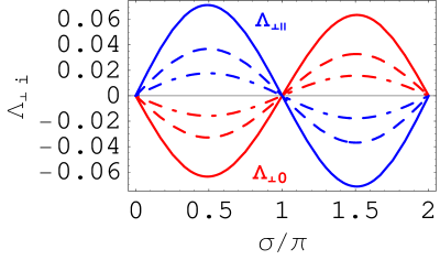
Figure 2: $\Lambda_{\perp i}$ as a function of $\sigma$ for $\tilde{m}_{1}=200\ {\rm GeV}$ and $\tilde{m}=2\ {\rm TeV}$. $\Lambda_{\perp i}$ are plotted in solid, dash and solid-dash lines for $m_{\tilde{g}}=300,\ 500,\ 800\ {\rm GeV}$.

In Fig. 2 we plot the observables $\Lambda_{\perp i}$ versus the NP weak phase $\sigma=\arg(c_{12}^{\prime})$ for three different values of the gluino mass $m_{\tilde{g}}=300,\ 500,\ 800\ {\rm GeV}$, with squark masses $\tilde{m}_{1}^{2}=(200\ {\rm GeV})^{2}$ and $\tilde{m}_{2}^{2}=2\tilde{m}^{2}-\tilde{m}_{1}^{2}$ with $\tilde{m}=2\ {\rm TeV}$. We note that the effects of NP can be at most a few percent, and tend to disappear as the gluino becomes heavier . This can be understood from Eq. (10) together with the expressions for $\Lambda_{\lambda\lambda}=a_{\lambda}^{2}+b_{\lambda}^{2}+2a_{\lambda}b_{\lambda}\cos\delta_{\lambda}\cos\phi$. In fact, the main contributions to $\Lambda_{\lambda\lambda}$ are proportional to $a_{\lambda}^{2}$ (tree level dominated) hence are of $O(1)$, while for $\Lambda_{\perp i}$ one has $O(b_{\lambda}/a_{\lambda})\sim O(0.01)$ at most, being suppressed by the ratio $P^{\rm NP}/T^{\rm SM}$ with $P$ and $T$ indicating respectively the penguin and tree terms.

We see that, for the particular model considered in this work, to observe NP effects by performing an angular analysis for the decay $B_{d}^{0}(t)\rightarrow J/\psi\,K^{*}$, one needs to be able to extract $\Lambda_{\perp i}$ with a precision of at least a few per cent. On the other hand, as stressed in Ref. LondonSinha , no tagging or time dependent measurements are needed to measure $\Lambda_{\perp i}$ since it appears with the same sign in both rates for $B_{d}^{0}(t)$ and $\bar{B}_{d}^{0}(t)$ (see Eq. (8)).

Following from the above considerations, it is evident that the decay $B_{d}^{0}(t)\rightarrow\phi K^{*}$ becomes really interesting. This decay, contrary to $B_{d}^{0}(t)\rightarrow J/\psi\,K^{*}$, is not tree level dominated. Rather, it is of pure penguin type, and in the model considered $a_{\lambda}$ and $b_{\lambda}$ are of the same order. This implies now that the observables $\Lambda_{\perp i}$ not only differ from zero if there are NP effects, but they are expected to be of $O(1)$, being the ratio $P^{\rm NP}/P^{\rm SM}\sim O(1)$. Obviously for the decay $B_{d}^{0}(t)\rightarrow\phi K^{*}$ the hadronic uncertainties play a more important role than for the decay $B_{d}^{0}(t)\rightarrow J/\psi\,K^{*}$, plaguing the theoretical prediction for $\Lambda_{\perp i}$. Furthermore, the strength of the transverse components are not yet understood.

For $B_{d}^{0}(t)\rightarrow J/\psi\,K^{*}$ decay, full angular analysis by the CLEO Collaboration CLEO shows that the $P$ wave component is small, ${\mid P\mid^{2}}={\mid A_{\perp}\mid^{2}}=0.16\pm 0.08\pm 0.04$, while the longitudinal component is around $50\%$, $\Gamma_{L}/\Gamma={\mid A_{0}\mid}^{2}=0.52\pm 0.07\pm 0.04$. Recent measurements for the longitudinal and transverse amplitudes have been also reported by both BaBar BaBar and Belle Belle Collaborations with the respective values ${\mid A_{\perp}\mid^{2}}=0.16\pm 0.03\pm 0.01$, ${\mid A_{0}\mid}^{2}=0.60\pm 0.03\pm 0.02$ and ${\mid A_{\perp}\mid^{2}}=0.19\pm 0.02\pm 0.03$, ${\mid A_{0}\mid}^{2}=0.62\pm 0.02\pm 0.03$. In Figs. 3 and 4 we plot respectively ${\mid P\mid}^{2}$ and $\Gamma_{L}/\Gamma$ as a function of the NP weak phase $\sigma$. It seems clear that both statistical and systematic errors need to be reduced by an order of magnitude to discriminate a nonzero value for $\Lambda_{\perp i}$ as predicted by the model considered. We expect that the error on the extracted value of $\Lambda_{\perp i}$ will be of the same order as the one on ${\mid P\mid}^{2}$ or $\Gamma_{L}/\Gamma$.

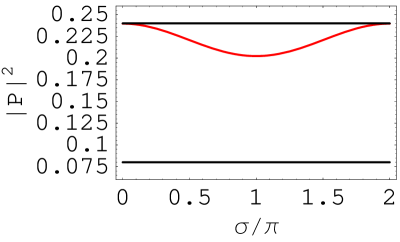
Figure 3: ${\mid P\mid}^{2}$ as a function of $\sigma$ for $\tilde{m}_{1}=200$ GeV, $\tilde{m}=2\ {\rm TeV}$ and $m_{\tilde{g}}=300\ {\rm GeV}$ compared with experiment.

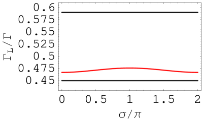
Figure 4: $\Gamma_{L}/\Gamma$ as a function of $\sigma$ for $\tilde{m}_{1}=200\ {\rm GeV}$, $\tilde{m}=2\ {\rm TeV}$ and $m_{\tilde{g}}=300\ {\rm GeV}$ compared with experiment.

We conclude this section by presenting the results for $\sin 2\phi_{1\lambda}^{\rm meas}={\rm Im}\left(\frac{q}{p}\frac{\bar{A}_{\lambda}}{A_{\lambda}}\right)$, where $\lambda=0,\parallel,\perp$ . If NP effects are present one will not be able to extract $\phi_{1}^{\rm mix}$ (the phase of $B_{d}^{0}-\bar{B}_{d}^{0}$ mixing which in general can be affected by NP) and the measured value of $\phi_{1}$, which will depend on the helicity of the final state, will differ from the real value of $\phi_{1}^{\rm mix}$ LondonSinha . In Fig. 5 we plot $\sin 2\phi_{1\lambda}^{\rm meas}$ as a function of the NP weak phase $\sigma$. As for the quantities $\Lambda_{\perp i}$, the effects of NP on $\sin 2\phi_{1\lambda}^{\rm meas}$ can be at most of few per cent. Deviations from $\sin 2\phi_{1}^{\rm mix}$ reach their largest value at $\sigma=\pi/2$ and are bigger for the transverse components, $\{\lambda=\parallel,\perp\}$. On the other hand deviations on $\sin 2\phi_{10}^{\rm meas}$, even if smaller, could be easier to detect because of the higher number of longitudinally polarized final states. On top of that by comparing $\sin 2\phi_{1}(B\rightarrow J/\psi K_{S})$  HeHou2 in Fig. 6 with $\sin 2\phi_{10}^{\rm meas}$, one can observe that deviations from $\sin 2\phi_{1}^{\rm mix}$ have opposite signs. This divergent behavior could in principle be easier to be observed than the single deviations.

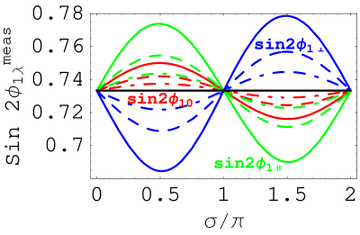
Figure 5: $\sin 2\phi_{1\lambda}^{\rm meas}$ as a function of $\sigma$ for $\tilde{m}_{1}=200\ {\rm GeV}$ and $\tilde{m}=2\ {\rm TeV}$. $\sin 2\phi_{1\lambda}^{\rm meas}$ are plotted in solid, dash and solid-dash lines for $m_{\tilde{g}}=300,\ 500,\ 800\ {\rm GeV}$. The black solid line corresponds to $\sin 2\phi_{1}^{\rm mix}=0.733$

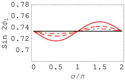
Figure 6: $\sin 2\phi_{1}(B\rightarrow J/\psi K_{S})$ as a function of $\sigma$ for $\tilde{m}_{1}=200\ {\rm GeV}$ and $\tilde{m}=2\ {\rm TeV}$. $\sin 2\phi_{1}(B\rightarrow J/\psi K_{S})$ is plotted in solid, dash and solid-dash lines for $m_{\tilde{g}}=300,\ 500,\ 800\ {\rm GeV}$. The black solid line corresponds to $\sin 2\phi_{1}^{\rm mix}=0.733$

V Conclusion

A supersymmetric extension of the SM with a light right-handed “strange-beauty” squark, a light gluino and a new $CP$ phase, seems to contain all the necessary ingredients to explain the recent $CP$ anomaly in $B_{d}\rightarrow\phi K_{S}$. In the same framework we have calculated possible NP effects to observables that can be extracted by the time dependent angular analysis of $B_{d}\rightarrow J/\psi\,K^{*}$. An important role is played by the quantities $\Lambda_{\perp i}$ with $i=\{0,\parallel\}$, which can be nonzero in the presence of NP even for very small strong phase differences. Our results show that deviations from zero can be at most of the order of a few percent, since it is suppressed by the ratios of the NP penguin amplitude to the SM tree amplitude. This obviously suggests that for decays which are pure penguins, like $B_{d}\rightarrow\phi K^{*}$, deviations from zero for the observables $\Lambda_{\perp i}$ are expected to be of order one.

The quantities $\sin 2\phi^{\rm meas}_{1\lambda}$ can also differ from the real value $\sin 2\phi_{1}^{\rm mix}$ because of NP effects. In particular $\sin 2\phi^{\rm meas}_{10}$ and $\sin 2\phi_{1}(B\rightarrow J/\psi K_{S})$ have opposite deviations from $\sin 2\phi_{1}^{\rm mix}$, and by comparing the two behaviors, NP effects could be easier to be observed than by looking at single deviations. As for $\Lambda_{\perp i}$, we found that deviations are of the order of few percent.

In conclusion, New Physics effects to $B_{d}\rightarrow J/\psi\,K^{*}$ from the model considered in this work are found to be too small to be observed at the current B factories. But because of the small NP effects, $B_{d}^{0}(t)\rightarrow J/\psi\,K^{*}$ remains a good mode for measuring $\sin 2\phi_{1}^{\rm mix}$.

References

(1) M.A. Giorgi , plenary talk at ICHEP04, August 2004,
Beijing, China.
(2)Y. Sakai, plenary talk at ICHEP04, August 2004,
Beijing, China.
(4) Chua, W.-S. Hou and M. Nagashima,
Phys. Rev. Lett. 92, 201803 (2004);
A. Arhrib, C.-K. Chua and W.-S. Hou, Phys.Rev. D 65, 017701
(2002).
(5) X.-G. He and W.-S. Hou, Phys. Rev. D 58, 117502 (1998).
(6)
R. Fleischer, Phys. Rev. D 60, 073008 (1999).
(7)
D. London, N. Sinha and R. Sinha, Phys. Rev. Lett. 85, 1807-1810 (2000);
D. London, N. Sinha and R. Sinha, (hep-ph/0304230);
D. London, N. Sinha and R. Sinha, (hep-ph/0307308), eConf C0304052:WG422 (2003);
D. London, N. Sinha and R. Sinha, (hep-ph/0207007); D. London, N.
Sinha and R. Sinha, (hep-ph/0402214).
(8) J.L. Rosner, Phys. Rev. D 42, 3732 (1959).
(9) N. Sinha and R. Sinha, Phys. Rev. Lett. 80, 3706 (1998).
(10) X.-G. He and W.-S. Hou, Phys. Lett. B 445, 344-350 (1999).
(11) G. Kramer and W.F. Palmer, Phys. Rev. D 45, 193-216 (1992).
(12) Y.-H. Chen, H.-Y. Cheng, B. Tseng and K.-C. Yang, Phys. Rev. D 60, 094014 (1999).
(13) M. Neubert and B. Stech, Adv. Ser. Direct. High Energy Phys.15: 294-344 (1998).
(14) P. Ball and V.M. Braun, Phys. Rev. D 58, 094016 (1998).
(15) Y. Nir and Sieberg, Phys. Lett. B 309, 337 (1993);
M. Leurer, Y. Nir and N. Seiberg, Nucl. Phys. B 420, 468 (1994).