Tachyonic preheating using 2PI-1/N dynamics and the classical approximation
Abstract:
We study the process of tachyonic preheating using approximative quantum equations of motion derived from the 2PI effective action. The scalar (Higgs) field is assumed to experience a fast quench which is represented by an instantaneous flip of the sign of the mass parameter. The equations of motion are solved numerically on the lattice, and the Hartree and 1/N-NLO approximations are compared to the classical approximation. Classical dynamics is expected to be valid, since the occupation numbers can rise to large values during tachyonic preheating. We find that the classical approximation performs excellently at short and intermediate times, even for couplings in the larger region currently allowed for the SM Higgs. This is reassuring, since all previous numerical studies of tachyonic preheating and baryogenesis during tachyonic preheating have used classical dynamics. We also compare different initializations for the classical simulations.
1 Introduction
In models of hybrid inflation [1, 2], one scalar field (the inflaton, ) triggers the symmetry breaking of a second (the Higgs field, )111Although our main emphasis is on the Standard Model Higgs, the discussion applies to a general scalar field. at the end of or after inflation [3, 4]. Typically the inflaton-Higgs coupling is introduced as an effective contribution to the quadratic Higgs term,
| (1) |
As the inflaton goes down, this effective mass changes sign from positive to negative, and as a result the Higgs field performs symmetry breaking by “rolling” into its broken phase minimum. The rolling off its unstable maximum is accompanied by an exponential growth of the amplitude of the momentum modes of the Higgs with , a process known as “spinodal instability” or “tachyonic preheating” [5]. Interactions end the transition, and the energy becomes redistributed through scattering into all the modes and other fields coupled to the Higgs. Eventually the system will thermalize to some temperature, which is called the reheating temperature of the Universe after inflation. Symmetry breaking and preheating are nonperturbative out-of-equilibrium processes, which are difficult to treat analytically [6, 7].
Numerical studies of tachyonic preheating [5, 8, 9, 10, 11, 12] and baryogenesis during tachyonic preheating [13, 14] apply the classical approximation to the out-of-equilibrium field dynamics, in which the evolution is determined by the classical equations of motion. The argument for making this approximation is that the important unstable low momentum modes acquire large occupation numbers; see [15, 16] for a detailed justification.
Whereas the instability and growth of the scalar field modes is due to the mass squared becoming negative, it is not obvious what happens when the Higgs is coupled to gauge fields. In [12, 13] it was seen that the low-momentum modes of the gauge field also acquire large occupation numbers, supporting the classical approximation for the coupled gauge-Higgs system. This large growth is essential for successful baryogenesis during (electroweak) tachyonic preheating [17, 18, 3, 13, 14], since these low-momentum modes are supposed to dominate the dynamics of the anomalous baryon number violating processes in the Standard Model (SM)(for a review, see [19]).
In an attempt to use a quantum description, while still incorporating the inhomogeneous nature of the typical non-perturbative field configurations of defects and anomalous baryon number violations, fermions in classical backgrounds were studied in [20, 21], and scalar fields in the Hartree approximation with inhomogeneous mean fields [22, 23, 24, 25], in 1+1 dimensions.
In this paper we apply an alternative description of out-of-equilibrium dynamics of quantum fields, using 2PI effective action techniques [26, 27]. In this approach equations of motion for quantum correlators are derived from a suitable quantum effective action (the 2PI effective action), in which the basic variables are the one- and two-point functions. Although the approach is formally exact, practical calculations require us to truncate an infinite expansion of loop diagrams (), defining a truncated 2PI effective action. The stationarity of the truncated effective action provides the -derived equations of motion. These equations include infinite loop resummations in the same manner as truncations of the Schwinger-Dyson hierarchy, and the two are closely related [28] (for other related work see [29, 30, 31, 32, 33]).
A crucial feature of -derivable approximations is that the derived equations of motion conserve global symmetries and associated Noether currents in time. In particular the energy is conserved. This is a useful feature when studying out-of-equilibrium processes where most other quantities such as particle distribution functions evolve in a complicated way. The conservation of energy applies not only to the full effective action, but to any level of truncation.
In [27] the formalism was numerically implemented for a relativistic scalar field in 1+1 dimensions for a study of the approach to equilibrium. Subsequent studies include [34, 35] in 1+1 dimensions, [36] in 2+1 and [37, 38] for fermions and scalars in 3+1 dimensions. The quantum -derivable scheme was compared to full and -derived classical approximations in [39]. Finally, the process of resonant preheating was studied in [40].
We report here on a study of tachyonic preheating in an model of scalar fields similar to the Higgs sector of the SM. However, since there are no gauge fields present, we expect Goldstone modes to appear. In the SM these would turn into the longitudinal modes of the massive gauge bosons. The results presented here may also have a bearing on effective pion dynamics in heavy-ion collisions.
In particular we will be interested in comparing results from the -derived equations to those obtained in the classical approximation. Initially we tried truncations of based on the weak coupling expansion, but the results were problematic because we run into instabilities. We record here results based on an expansion in , with the number of fields (here ), following [35, 41]. This expansion is systematic and the numerical algorithm is stable even for very large occupation numbers [35, 40].
2 Tachyonic preheating
The system is described by the classical action
| (2) |
with the energy density at , and , summation implied. In equilibrium at zero temperature, the system is in a broken-symmetry phase if , with
| (3) |
where is a unit vector, . The particles in this phase are massless Goldstone bosons corresponding to the modes transverse to , and the Higgs boson corresponding to the longitudinal mode, with mass . A feeling for the strength of the interaction may be obtained from the amplitude for the scattering of Goldstone bosons (, assuming ):
| (4) |
This leads to an S-wave unitarity bound [42]. For , the triviality bound obtained with the lattice regularization is about two-thirds of this, [42, 43]. In the Standard Model, GeV, and a Higgs mass GeV would give . This looks like a weak coupling, but such a Higgs mass is near the upper end of the interval set by the constraints from radiative corrections [44].222 On the other hand, a potential application to heavy-ion collisions using effective pion dynamics, where the role of the Higgs is played by the sigma-resonance, MeV, MeV, would require very strong coupling, .
The coupling of the model to the inflaton may be described by the replacement in the action (2). The spinodal instability occurs when the coefficient of the quadratic term in the potential flips sign. Ref. [15] contains a detailed analysis of the initial subsequent development, and a justification is given of a classical approximation after the instability has sufficiently progressed; see also [45]. We go to the limit where the flip happens infinitely fast, a quench, which we model by
| (5) |
We assume that the initial state of the system is the ground state in a quadratic potential just before the quench, a free “vacuum” , with correlators333We use the Fourier decomposition in a periodic box of linear size .
| (6) | ||||
| (7) | ||||
| (8) |
where . As detailed in [16], we can then solve for the evolution of these correlators in the quadratic approximation () as a function of time. The result is reproduced here for convenience,
| (9) | ||||
| (10) | ||||
| (11) |
with . The derived occupation numbers and frequencies are
| (12) |
It follows that modes with grow exponentially with
| (13) |
We will use equations (2) – (2) for comparison at early times.
Also in more general situations [22, 46, 24, 12] the above give an instantaneous characterization of frequency, assuming a translation and rotation-invariant density matrix, and they provide for a corresponding definition of annihilation operators as (concentrating on one real field) , and creation operators , such that . Hence the have a natural interpretation as occupation numbers. For free fields in equilibrium the and coincide with the standard particle numbers and energies. The are given by . For large the non-zero commutator corresponding to the imaginary part of (2) becomes unimportant in expectation values of suitable observables (e.g. particle numbers), which suggests that the classical approximation should be good. Ref. [15] stresses that is the important criterion for classical behavior. For our initial state and are not independent, but satisfy , so with , whenever , and for large the two become very close. For precise formulations of the classical approximation in terms of probability distributions of initial conditions, see [15, 16].
The initial state is symmetric, which implies that the mean field stays equal to zero also for the general case ,
| (14) |
and that the correlators can be written as
| (15) |
As the grow, eventually the back-reaction from the quartic term will become important and the evolution will deviate from the quadratic approximation. As we will see below (section (7)), this happens around the time when ()
| (16) |
Since
| (17) |
we expect the occupation numbers to be non-perturbatively large
| (18) |
which suggests that a simple loop expansion in powers of the coupling is unreliable for tachyonic preheating.
3 Broken phase and finite volume
After the initial tachyonic preheating the system will go to equilibrium and thermalize. To estimate the final temperature , consider a simple approximation in which the initial energy density, , is transfered to a free gas of massless Goldstone bosons and one massive radial mode of mass . This approximation is expected to be reasonable for weak coupling, provided is far from the critical temperature at which the transition between the broken and symmetric phase occurs. Using , the temperature is then given by
| (19) |
For , this gives (the large limit would give ). On the other hand, the transition temperature can be estimated in a simple one-loop approximation [47],
| (20) |
which gives , for and . This also agrees well with Monte Carlo results [47]. Since the estimated final , we expect the system to end up in the broken-symmetry phase.
Our simulations are performed in a periodic box of size . It is well-known that quantum tunneling effects prevent spontaneous symmetry breaking in finite volume. Hence, , but this does not mean that physical effects of symmetry breaking cannot manifest themselves in finite volume. In fact, the Goldstone bosons may cause relatively strong finite size effects and slow thermalization.
The standard way to define is to add a symmetry breaking term to the action,
| (21) |
which pulls into the direction , and then evaluate
| (22) |
Aided by finite-size scaling analysis this method has been used fruitfully in Monte Carlo studies [48]. The order of the limits in (22) is important. However, reversing the order (working at ), a lot can be learned from analysis at finite size [49].
A proper finite-size scaling analysis is outside the scope of our present explorative study. Instead, we shall work at reasonably large volumes, . As a guideline for interpretation of the numerical results at relatively large times (close to equilibrium), we take the tunneling into account by simply averaging the infinite-volume broken-symmetry correlators over all internal directions:
| (23) | |||||
| (24) | |||||
| (25) |
where G and H denote the Goldstone and Higgs contributions. Hence, after having settled sufficient into equilibrium, the symmetric Green function is expected to have both Goldstone and Higgs contributions, and a zero-momentum mode expressing the condensate.
4 The 2PI effective action and equations of motion
We use the Schwinger-Keldysh formalism, in which the fields live on a contour running from to some time and then back to . Time integrations and time ordering are along this contour. At the two times there are functional integrations implementing the density matrix that specifies the initial state. The functional is a sum of 2PI skeleton diagrams with bare vertices and full propagators corresponding to the initial state , see figure 1.

The full propagator is a stationary point of the effective action. Taking the functional derivative gives the equation determining ,
| (28) |
with the self-energy,
| (29) |
Multiplying (28) by turns it into an integro-differential equation,
| (30) |
Together with the equation for , which follows from , this determines in a self-consistent way, since the self-energy is itself a functional of , eq. (29). Since will be identically zero because of the symmetry of the initial state, we now specialize to this case.
The delta function in (30) for can be taken care of by introducing and according to
| (31) |
where the step functions refer to the time label along the contour . The ‘statistical function’ and the spectral function correspond to the real and imaginary parts of or ,
| (32) | |||
| (33) |
In operator language they correspond to
| (34) |
The functions and are real and have the symmetry properties
| (35) |
The canonical commutation relations imply
| (36) |
Equation (30) now leads to coupled integrodifferential equations for and , supplemented by initial conditions depending on the initial density matrix. These equations preserve the properties eq. (35, 36), and conserve energy for any choice of truncation of .
One would like to know if truncations of lead to solutions for that describe massless Goldstone bosons when the system is in the broken-symmetry phase444Such Goldstone bosons are still present in our case of zero mean field, cf. section 3.. Generically this is not the case [41, 50]. However, one can introduce the 1PI effective action
| (37) |
with the solution of (28) for given mean field , and define a Green function (called ‘external’ in [50]) in the usual way from :
| (38) |
Then the usual derivation of Goldstone’s theorem in terms of applies to , it has zero eigenvalues at zero momentum [41, 50]. Without approximation the Green functions and coincide, but this is no longer true for a truncated . The difference between and depends on the functional derivative [50]. This is a three-point function (given by the solution of a non-trivial integral equation) that vanishes in our case of zero mean field. Therefore, we do expect to describe massless Goldstone bosons.
At first we tried a truncation of the effective action based on the loop expansion, by keeping the diagrams shown in figure 1, for . However, this lead to severe instabilities before the transition was completed, for weak and also for stronger couplings, which we were unable to cure. We interpret this as a breakdown of an expansion based on the smallness of , because of the non-perturbatively large occupation numbers expected during the instability (eq. (18)). We then turned to an expansion of the 2PI effective action, not in powers of the coupling , but in terms of . Following [35] we expand to Next-to-Leading Order (NLO) in . The explicit form of the resulting equations can be found in [35] (see [41] for the case of non-zero mean field).
5 Numerical implementation
We discretize the model on a space-time lattice with the action
| (39) |
Here the lattice spacings are and in the spatial and time directions, , and similarly for spatial derivatives. We use periodic boundary conditions, with volume is . In the following we shall use lattice units, and write for the dimensionless time-step (). The coupling and mass parameter are bare parameters to be determined below. At tree level, and in the broken phase. The lattice version of the squared momentum is given by,
| (40) |
( is chosen even). Plotting data as a function of the lattice momenta rather than continuum corrects for most of the lattice artifacts.
As explained in [35], truncating the expansion at NLO and specializing to a homogeneous system () with zero mean field, leads to the equations of motion:
| (41) | ||||
| (42) |
with , and similar for , and with555When practical, we shall use a notation in which, for instance, .
| (43) | ||||
| (44) | ||||
| (45) |
The functions and represent the summation of bubble diagrams included at NLO [35]
| (46) | ||||
| (47) |
Note that and contain an overall factor , they would start at order upon solving the above equations by perturbation in . The contribution of order (coming from the first diagram in figure 1) is purely local (non-zero only for ) and contained in defined in (43). During the numerical evolution we have to solve for and parallel to solving for and . Although eqs. (5, 5) look implicit, by doing things in the right order and taking advantage of the symmetries
| (48) |
they can be solved explicitly. The energy functional is given by
| (49) |
where ‘sub.’ is a subtraction. Ideally, this subtraction is such that the energy density is zero in the vacuum (the zero-temperature ground state), but its evaluation requires a non-trivial minimization. In practise we set the energy density to , for the initial state (6–8).
5.1 Hartree approximation
In addition to the NLO-1/N approximation, we study the Hartree approximation, which results from taking into account only the first diagram in figure 1. This means leaving out all time integrals, and the , keeping only the first line of eqs. (5) and (5), with defined by eq. (43). Notice that this is not the Leading-Order (LO) approximation in 1/N, since the coefficient of the local self-energy is as opposed to for LO-1/N. Neither of the two includes non-trivial scattering in the dynamics and they give qualitatively the same results. We use Hartree dynamics only for comparison.
5.2 Initial conditions
We restrict ourselves to initial conditions for which the density matrix is gaussian. This assumption is equivalent to the initial state being completely described in terms of (one- and) two-point functions [29]. Consequently, an initial condition is a choice of initial ’s, ’s and (which in this case is zero). We need to specify
| (50) | ||||
| (51) | ||||
| (52) |
in addition to
| (53) | ||||
| (54) |
where we used for a homogeneous system. This also allows us to go to momentum space and define666The Fourier transforms are given by , etc.
| (56) | ||||
| (57) | ||||
| (58) |
given a choice of “occupation number distributions” , and dispersion relation . We specialize to the case , noting that in equilibrium this correlator is zero. As mentioned in section 2, we assume that the system is initially in the state corresponding to the ground state before the quench, which we approximate by the free-field vacuum in the symmetric-phase,
| (59) |
Notice that we use the renormalized quantity in the initial condition, in accordance with section 2. Also, since this initial state is a free-field vacuum, it is not the true vacuum of our interacting system in the symmetric phase.
5.3 Choice of bare parameters
The renormalizability of -derivable approximations was studied in [51, 52, 53, 54, 55]. We assume the NLO-1/N approximation to be renormalizable, in the sense that we can choose the coefficients in the discretized equations (5–5) in such a way that the lattice spacing becomes exceedingly small 777This may imply a more elaborate set of parameters than just and . At worst, an independent parameter may be needed for every contribution to the truncated (e.g. every diagram), since there is no symmetry relating various contributions. In practise this is not a problem for sufficiently accurate truncations [55]. – loosely called ‘the continuum limit’.888Such terminology ignores triviality. We will not study lattice-spacing dependence but do want to choose the parameters and such that the relevant length scale in our simulation is larger than the discretization scale, i.e. .
For this purpose we implement renormalization at one loop order. At weak coupling, mass renormalization is important, but not coupling renormalization. Two-loop effects are also small, and the bare mass in the equation of motion is therefore estimated in one-loop renormalized perturbation theory as
| (60) | |||||
| (61) | |||||
| (62) |
in the continuous-time and infinite-volume limit. In (60) the plus (minus) sign refers to the symmetric (broken) phase. The one-loop self-energy refers to the symmetric phase, the broken phase should give the same divergent contribution as and a small difference in the finite contribution. An idea of the size of the coefficients may be obtained from a calculation on a symmetric () lattice in imaginary time [56],
| (63) |
Similarly, the bare coupling can be estimated by the one-loop expression [56]
| (64) |
(where is defined as the value of the four-point vertex function at vanishing external momenta). For the maximum coupling that we use () and lattice spacing , the difference between and is less than 10%. In practise we simply choose as if it were the renormalized coupling. In our simulations we use the bare coupling in (60), i.e. on a -site lattice, in lattice units,
| (65) | ||||
| (66) |
Given the input parameters and , the output physics is of course not known precisely, it is determined by the -derived equations. For example, the mass of the (unstable) Higgs particle will differ from the tree graph value . Similarly, the renormalized coupling will not satisfy the relation (64) precisely ( may also be defined in terms of the vev by where the vev may be identified from the low-energy scattering amplitude of the Goldstone bosons, cf. (4)). But the differences are expected to be small, and they can in principle be determined numerically.
In our out-of-equilibrium study there is another dimension-full scale: the mass in the initial conditions (59). It is the renormalized mass in the symmetric phase, and it is this mass that we use in (65) for choosing . We have to keep in mind that the gaussian approximation in the initial conditions and the suddenness implied by the quench may lead to divergencies in the pressure near , in the continuum limit, see e.g. [57]. These may be dealt with by adjusting the initial density matrix, but it would be better to avoid the instantaneous quench and use a more realistic model of the transition. Such divergencies do not appear to be important in our simulations at finite lattice spacing.
5.4 Observables
We follow the evolution of and the energy, eq. (5), and calculate occupation numbers and frequencies through the inverted version of eq. (56),
| (67) | ||||
| (68) |
The quantities and coincide with the true particle occupation numbers and frequencies when applied to a free field in equilibrium, and have proven to be very useful out-of-equilibrium in interacting theories as well [22, 46, 24, 12]. The correction takes care of errors associated with the time discretization on the lattice. It is given by [24]
| (69) |
In the present case we argued in section 3 that the two-point function receives contributions from both the Higgs and the Goldstone modes, so in this respect the and are compound observables.
After some initial transients, the system will approach thermal equilibrium, although this may take a long time because of critical slowing down: the scattering of the Goldstone bosons becomes suppressed for momenta smaller than the Higgs mass, cf. (4). The approximate expression (25) for in terms of and provides a guide to what form we may expect for the and defined in (67):
| (70) | |||||
| (71) |
where, assuming that the individual Higgs and Goldstone modes have thermalized to a Bose-Einstein (BE) distribution,
| (72) |
and and are to be interpreted as the condensate and effective Higgs mass at temperature . We have allowed for a time dependent , although in (71) we have neglected its time derivatives. Close to equilibrium we expect the change in to be very slow (, see figure 12 below). At low momenta () the Goldstone bosons will clearly dominate. Note that in finite volume the condensate appears only in the zero mode of , and there is no zero mode in the Goldstone contribution : it is represented by the global rotations making up the average in (24).
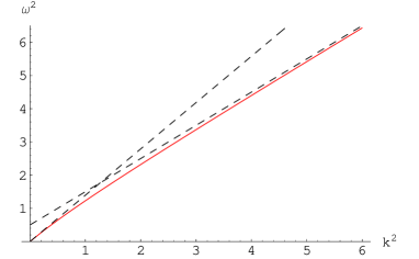
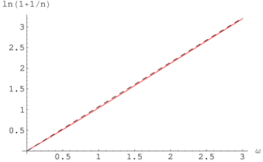
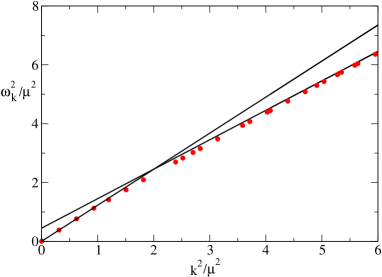
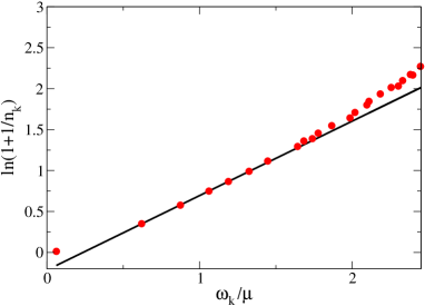
In figure 2 (left) we have plotted the resulting at the expected temperature found in section 3 for , . The straight lines correspond to the asymptotes
| (73) | |||||
| (74) |
This latter formula may provide an estimate of the effective Higgs mass, although the emphasis on the large momentum region is questionable. A better way to determine should be to find the position of the peaks in the Fourier transform of the spectral function, as done in 1+1 dimensions in [34]. Figure 2 (right) shows the compound particle number from (67)–(72) for the same parameters as for in the left-figure. Plotted is versus , which would be a straight line with slope if were a Bose-Einstein distribution with zero chemical potential. The deviation from BE is hardly visible, which suggests that such a plot is also useful for judging the approach to equilibrium, even for the compound particle number. For a BE with a non-zero chemical potential , we would see an intercept with the -axis equal to . For the compound particle number this also applies with the understanding that the intercept gives the chemical potential of the Goldstone particles, .
For sufficiently large volume the condensate follows from the zero mode of ,
| (75) |
which has been found to give good results compared to a more rigorous procedure based on (22) and finite-size scaling [48]. The relative correction
| (76) |
(which may also be estimated from ) is tiny: for and of order 100 it is only of order .
In the classical approximation we found [16, 14, 12] the observable useful for monitoring the tachyonic transition, and we have used it here as well. Its quantum analog is divergent in the continuum limit and needs a subtraction. We have taken this to be its initial value ( in lattice units cf. (56), (59), (66)). The difference then vanishes at time zero and at late times (70) indicates that
| (77) | |||||
where the second line refers to units. The last integral is logarithmically divergent as (at two-loop accuracy there may be also quadratic divergencies). A different subtraction, e.g. such that the result is finite in the broken-symmetry vacuum state, may render it divergent as . This is an example of the artifacts introduced by the suddenness of the quench. Nevertheless, for the lattice spacings that we use these remaining divergencies are negligible. For example, in lattice units the last integral in (77) is only 0.00922 for .
We also compute the ‘memory kernels’ in the equations of motion (5)–(5), the self-energies and , which can be compared with perturbative estimates. For long runs, finite computer memory requires us to “cut off” the self-energy (in terms of the functions ), by keeping the memory kernels only some finite range backwards in time (i.e. , ). The size of the self-energies will help us determine whether we have cut off late enough for the discarded memory integrals to be negligible for the dynamics. A too early cut-off also shows up as a non-conservation of energy. In all the runs presented here, the energy is conserved to within two percent. At early times its fluctuations are due to time discretization errors. At very late times, the effect of cutting off the memory kernel can add up to a very slow drift in the energy, but still within the two percent band. Keeping the whole kernel (say, for lattices of smaller spatial extend) there is no such drift, and we have checked that later cut-offs make the drift smaller. Our choices of memory cut-offs reflect a compromise between exact energy conservation, lattice sizes, computer memory and especially CPU time, and the wish to study reasonably long time evolution.
6 The classical approximation
In the classical approximation, a set of classical initial realizations is evolved using the classical equations of motion. These realizations are drawn from an ensemble of initial conditions that reproduce the initial quantum correlators in a classical approximation. In the case of tachyonic preheating we do not have to wait for the correlators to become classical if the couplings are weak – we can go back all the way to time zero and reproduce eqs. (2), (2), (2) at ,
| (78) |
See [16] for a more detailed justification of this procedure. Note that the stable modes are initialized to zero. In section 7.3 we comment on the case where all the modes are initialized according to the initial quantum correlators, including the modes . Observables are then averaged over the sample, giving an approximation of the quantum observable,
| (79) |
To compare with the derived approximation, we perform classical simulations starting from the same lattice Lagrangian as in the quantum case, eq. (39). The classical equation of motion reads
| (80) |
The classical simulations use the same lattice sizes and spacings as in the quantum case. As observables we use
| (81) |
which is the analog of the quantum correlator , and the energy
| (82) |
Comparing to we should keep in mind that the latter is divergent in the continuum limit, whereas classically
| (83) |
We therefore compare (cf. the discussion in the previous section)
| (84) |
ignoring the small difference at time zero.
We also calculate occupation numbers and frequencies from the and correlator in a manner similar to eqs. (67,68) (without the ‘1/2’),
| (85) |
We average over with the same length . This gives better statistics, and since the system is homogeneous and isotropic as for the quantum case, the correlators depend on the length of , apart from lattice artifacts.
In the classical approximation we expect equipartition to occur after very long times, for which the occupation numbers for the Goldstone and Higgs modes are given by
| (86) |
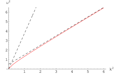
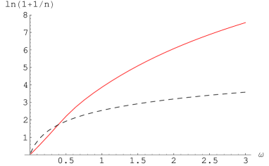
The Rayleigh-Jeans temperature is determined by classical equipartition, , or with , . In our longer-time simulation we used and , which gives the low value . The corresponding guiding plots for the compound frequencies and particle numbers are shown in figure 3. The deviations from the BE case in the compound-frequency plot appear limited but significant. The greatest deviations appear in the compound-particle number case: the curvature caused by plotting (instead of the more appropriate ), done for diagnostic reasons, which cannot only be ascribed to a dominating Goldstone contribution.
7 Numerical results
7.1 Early times: Tachyonic instability
We first describe simulations during the initial tachyonic transition on a lattice with sites, lattice spacing , volume , time step , with weak coupling . The number of fields .
We compare four different approximations: 1) The analytical result in the quadratic approximation (eqs. (2), (2), (2)) ; 2) Hartree (cf. sect. 5.1); 3) 1/N to NLO (eqs. (5) – (5)); and 4) classical (eq. (80)). In the classical case, we average over an ensemble of 400 configurations. For the 1/N-NLO case relatively short times allow us to keep the whole memory kernels in the self-energy.
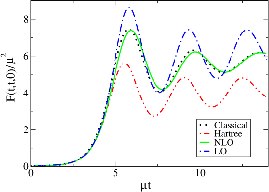
In figure 4 we show the evolution of the subtracted for the NLO, Hartree and classical (eq. (84)) case. We have also included LO-1/N for comparison. The NLO and classical agree well with each other (and settle later near the zero-temperature vev, ). The Hartree result is remarkably lower than the others, while the classical approximation seems to work very well. The Hartree being lower appears to be the result of the choice of coefficient of the local term, the choice of . In the limit of large we recover the LO result, which for overshoots compared to the classical and NLO. Below, we will discard the LO approximation, since it is qualitatively the same as Hartree.
Figure 5 shows the evolution of the compound occupation numbers for the Hartree approximation (green/grey) compared to the quadratic approximation (black). At early times the agreement is very good but eventually back-reactions enter and the spinodal growth ends. As is well known, the homogeneous Hartree approximation does not include non-trivial scattering, and essentially no energy is re-distributed to modes of momentum higher than .
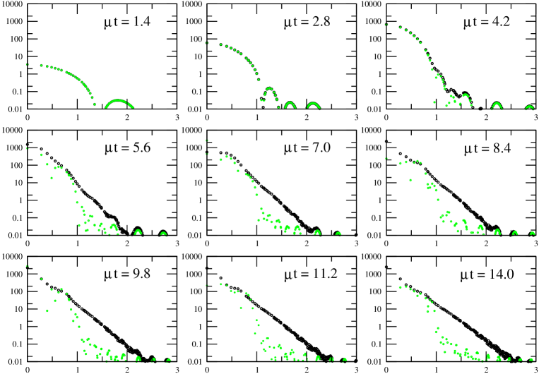
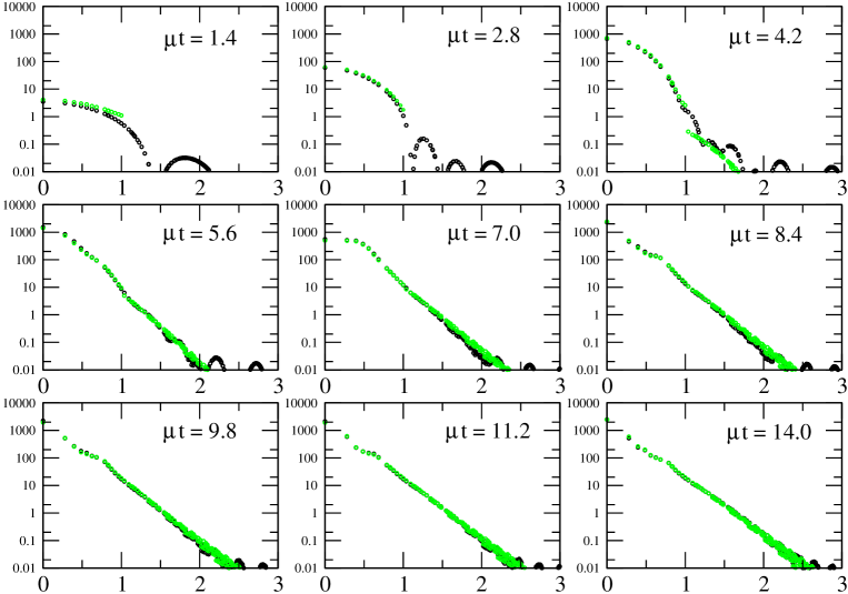
Figure 6 compares Hartree (green/grey) to NLO (black) dynamics. Initially they agree very well. As the back-reaction kicks in, scattering processes included in the higher loop diagrams of NLO allow re-scattering of energy into the higher momentum modes. The spinodal growth ends roughly around , when (cf. figure 4), at which time defined in (43) goes through zero (as anticipated in (16)).
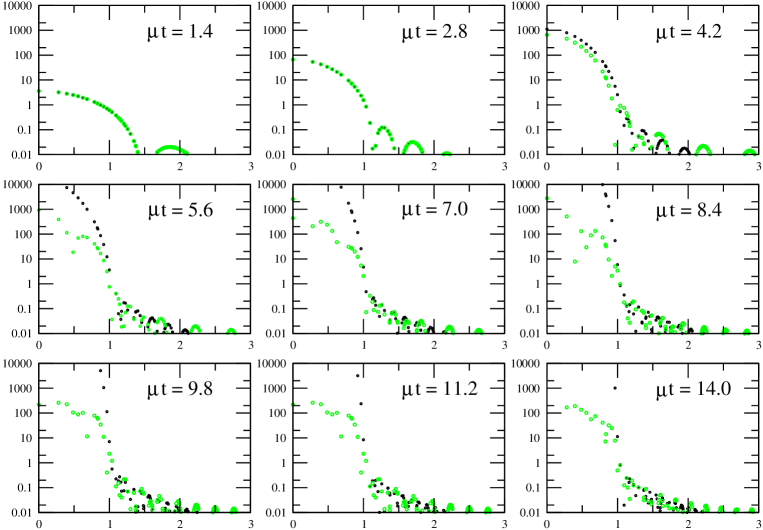
In figure 7 we compare the NLO (black) result to the classical (green/grey) case. In the classical case only the unstable modes are initialized, which is why the stable modes are outside the picture initially (having ). In the quadratic approximation the evolution for classical modes and quantum mode functions is identical, so we expect the unstable modes to also be described by eq. (12). This is indeed what we see, and as back-reactions kick in, the stable modes become populated and “hook up” with the unstable ones to reproduce the low-momentum part of the distribution of the NLO case very well. Turning things around, the full dynamics of the classical evolution is well described by the truncated NLO quantum dynamics.
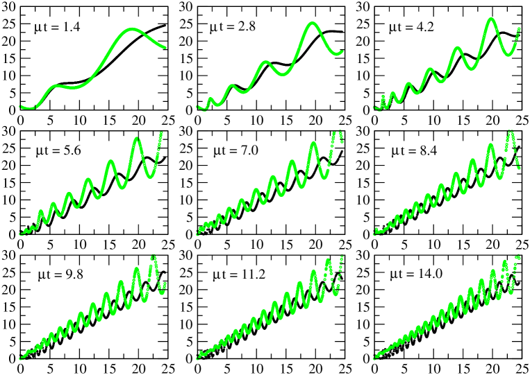
Figure 8 shows the compound-dispersion relation during the transition at NLO. The low momentum modes are again well approximated by the gaussian equations (2, 2, 2), and although the quantitative agreement is lost for large momentum modes and larger times, the qualitative picture is well understood. For the Hartree case the picture is roughly the same at these early times. The averaging in the classical case was seen to smear the oscillations.
7.2 Intermediate times: approach to equilibrium
As interactions become important the spinodal transition ends. We may expect scattering to result in equilibration of the system. This does not happen in the Hartree approximation, but the inclusion of the NLO diagrams has been seen in previous studies to lead to thermalization, in 1+1, 2+1 with scalar fields and in 3+1 dimensions including fermions [58, 36, 37, 38]. In the present case, however, the suppression of the scattering of the massless Goldstone bosons at low momenta (cf. (4) may lead to slowing down of the thermalization of these modes. In the classical approximation, we expect classical equipartition to take place after a very long time. For intermediate times, it was seen in [12] that the low momentum modes of a system including gauge fields could be well approximated by a Bose-Einstein distribution, allowing for a determination of an effective temperature and chemical potential, even with classical dynamics.
To study the longer time behavior we performed simulations on a smaller lattice, , again with , , , but with a larger coupling . For the classical simulations we averaged over 1000 realizations of the initial conditions. For the quantum NLO case we cut off the memory kernel at . This gave no problems with energy conservation and we believe it does not affect the evolution much. With the enhanced back-reaction of the larger coupling we expect smaller after the transition, since the spinodal transition does not last as long. Instead of a zero mode reaching previously , we have here only . This still amply satisfies the criterion for classicality.
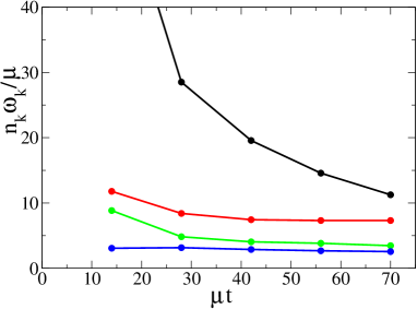
In figure 9 we see the evolution of the compound dispersion relation. In the NLO case, the oscillating behavior generated during the transition (figure 8) is washed out by scattering to a straight line. A close-up at the latest time the NLO compound-frequency plot figure 11 appears to show the behavior anticipated in figure 2. The asymptote to the data at larger momenta indicates an effective Higgs mass (cf. (74)), somewhat lower than the zero-temperature value. At finite temperature in the broken phase we do expect a smaller Higgs mass, since the condensate is also smaller than at zero temperature (see figure 12, left). Inserting the finite temperature in the expression for the mass , one finds .
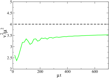
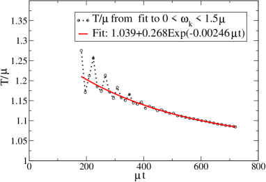
The slope of the line through the origin and the first data point is at this time , quite a bit off the anticipated (see figure 2). With this slope and effective mass, no choice of satisfies (73). Apparently we are not sufficiently close to equilibrium, in particular in the low-momentum region. Figure 10 shows the evolution of the compound occupation numbers at later times. At NLO, redistribution is clearly taking place, and power is being moved towards higher momentum modes. In the Hartree approximation nothing much happens. The classical case also shows redistribution over the modes and mimics the quantum evolution nicely at low momenta for not too long times. At the latest time some concaveness appears to show up, perhaps indicating classical equipartition (cf. figure 3). We come back to this in more detail in the next section. In figure 11 we show a close-up of the NLO case at the latest time. We include a fit to the low momentum region (neglecting the zero mode). As discussed in section 5.4 (see figure 2), such a straight line represents a thermalized state, with the slope equal to , and intercept equal to the effective (Goldstone) chemical potential. For this fit we find and . The temperature is higher than our free-field estimate (19). This is not surprising since the high-momentum range is still under-populated at this time, compared to the thermal state. Figure 12, right, shows the evolution of this temperature in time. An exponential fit suggests an asymptotic final temperature of around .
7.3 Choice of classical initial conditions
As an aside we comment on the choice of initial conditions for classical simulations of tachyonic preheating. Two approaches have been put forward, one used by many authors (see e.g. [9, 10]), in which all modes are initialized with the “quantum half”, i.e. also in eq. (78), the other [59, 16, 14, 15, 13], in which only the unstable modes are initialized, as we did in the previous section.
It is clear that initializing all the modes, we risk running into an ultraviolet problem in the continuum limit . In the classical approximation, equipartition may cause the divergent energy sitting in the high momentum modes to flow into the low-momentum range and generate a too high temperature, see [59], and [60] for a study with massless gauge fields. However, this did not happen on short to intermediate time scales in our -Higgs study in which the gauge fields were massive [12], and also for scalar fields with only self interactions the problem shows up on a much larger time scale than for massless gauge fields [60]. Thermalization for scalar fields is rather slow and it is possible that the high-momentum modes never come into play on time-scales relevant to numerical simulations of phase transitions. The important criterion must be which initialization method reproduces the quantum evolution of the low momentum modes more closely, in terms of occupation numbers and equilibration times. We shall take the NLO case as representing the quantum result.
It is also important to keep in mind that, when attempting to calculate topological quantities such as the Chern-Simons number in models which include gauge fields, the lattice implementation is very sensitive to ultraviolet fluctuations. In simulations of baryogenesis, Chern-Simons number is a crucial observable, since it is simply related to the generated baryon asymmetry. This was in fact one of the motivations for introducing the initialization restricted to the unstable modes [16, 14].
When initializing all modes, the effective mass receives a contribution from all these modes (divergent in the continuum limit), compared to when only the unstable modes are initialized, in a way analogous to the quantum vacuum case. We should therefore introduce a counterterm for the mass in a way similar to the quantum case [9],
| (87) |
where again is given by eq. (66). For consistency, we also define the occupation numbers according to the quantum equation,
| (88) |
rather than through eq. (85), and the energy and pressure also have to be renormalized.
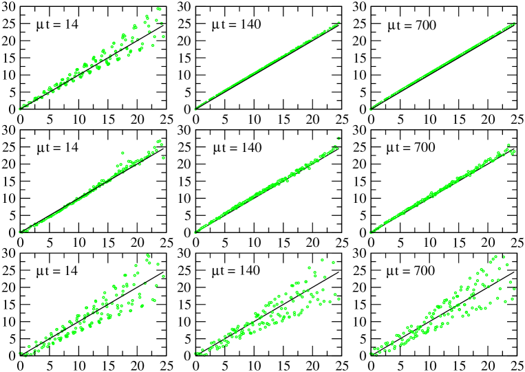
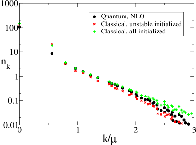
The result is shown in figure 13, where the two classical approaches are compared to the NLO quantum case. Just after the transition (, ), the classical with only the unstable modes initialized follows the quantum case nicely in the low momentum region. This is also the case when initializing all the modes. We conclude that as long as the simple renormalization procedure eq. (87) is imposed, the number of modes initialized is not crucial at these early times, when classical equilibration has not set in yet.
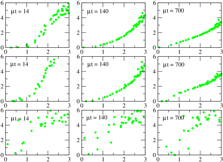
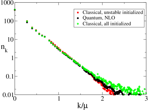
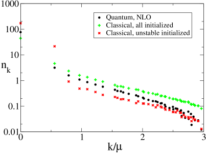
For longer time (figure 14 left plot, , , ), we see that both types of initialization approximate the quantum behavior, with the ‘all initialized’ doing somewhat better than the ‘unstable only’. We do not expect the classical modes with occupation numbers less than one to be correct. Surprisingly, the very lowest modes with are also off in both cases. At even longer times (figure 14 right plot, ), the agreement is only qualitative, with either intitialization scheme performing badly. For only the unstable modes initialized, we see that the occupation numbers are lower than for NLO, presumably because of the lack of scattering with the high momentum (stable) modes. In the quantum case there is apparently still some scattering going on with the quantum fluctuations of the initial free ‘vacuum’. When initializing all the modes, this effect appears to be incorporated in the ‘all initialized’, but it seems to be too large. This could also be the reason that the zero mode is lower than for NLO. Eventually, we expect to approach the equilibrium value following from (70, 71), , for the parameters of the simulation.
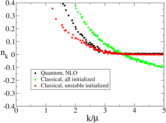
There is an interesting aspect to this. In figure 15 we see the high momentum modes at the same time as figure 14, right; shown is vs on a linear scale. In the quantum case, the quantity is always positive and here close to zero, as we would expect. This is a consequence of the standard quantum commutation relation. The power in the vacuum fluctuations, the “”, cannot be extracted and moved to other modes. For the classical case with only unstable modes initialized, the are also manifestly positive numbers, and close to zero. In the classical case with all modes initialized, there is no principle which enforces that should be larger than , and we see that it ends up negative for . This illustrates the problems associated with renormalization in classical field theory out of equilibrium. Only for short times, as we have seen, or in equilibrium [61, 62, 63], such a procedure has a limited validity, albeit with initial-state or temperature-dependent counterterms.
7.4 Effective temperature in the unstable modes
In [17, 13] the baryon asymmetry in scenarios based on electroweak preheating was estimated using equilibrium concepts, such as the sphaleron rate at an effective temperature and an effective chemical potential for Chern-Simons number. The idea was that the large occupation numbers in the unstable modes would lead to early equilibration amongst these modes at an effective temperature . Such an approach might enable one to bypass the more difficult numerical simulations using CP violation in the equations of motion (we note that the comparison made in [14] did not seem to support this idea at a quantitative level). It is therefore of interest to estimate such an effective temperature here.
Equilibrated modes with high occupation numbers have an effective temperature given by the classical formula , independent of , and one estimate of the effective temperature follows from energy conservation and dominance of the unstable modes [17],
| (89) |
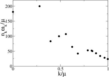
With GeV, , this gives a high GeV (1820 GeV), for (6). The actual of the individual modes as obtained from the correlator ( Higgs- plus Goldstone-contributions, as in (71)), is shown in figure 16 (left) at time , for the lattice with . We see that the unstable modes have not equilibrated much yet, since the effective temperatures vary significantly from mode to mode (the zero mode should be ignored as it contains the condensate). Note that the corresponding particle distribution is shown in the lower-right panel of figure 7. As the panel in the latter figure shows, the modes near the border of the unstable region () are not initially highly populated, and also at time their effective temperature is much lower than the simple estimate (89). The effective temperature in the modes near in figure 16 (left) is about 100 ; the average over all unstable (non-zero) modes gives , about half the estimate (89) for , .
The effective temperatures at later times are shown in figure 16 (right). Equilibration is evidently slow even in the unstable momentum region, which is perhaps to be expected because of the suppressed scattering of Goldstone bosons at low momenta. In a more realistic setting, the gauge fields and other degrees of freedom of the SM will lead to more efficient thermalization and lower effective temperatures. In the study [12] the SU(2) gauge fields were taken into account, which led to effective temperatures at (cf. figure. 15 and Table 2 in ref. [12]), for .
8 Conclusion
The -derived –NLO approximation performed well in this study of a tachyonic phase transition, for the model at reasonable couplings999At stronger couplings we did see annoying instabilities similar to what we found in approximations based on the weak-coupling expansion of . In this sense the larger coupling used in Sect. 7 is not very weak.. It is reassuring that the classical approximation agrees so well with the quantum case, not only during the transition, were we used a smaller coupling (with the accompanying larger particle numbers), but also subsequently for not too long times, where we used the larger coupling. In a sense, the classical and NLO approximations support each other, the first taking into account all non-linearities without further truncation and the second including quantum scattering right from the beginning. For longer times the quantum computation is of course superior as it does not suffer from Rayleigh-Jeans ambiguities.101010For some problems one may have to face a non-uniformity of large versus large [64].
Because of the symmetry of the initial state, the mean field was zero at all times. Consequently there was no conflict with Goldstone’s theorem – we consider the numerical evidence for massless particles to be quite convincing.
Critical slowing-down of thermalization is expected to take place as a result of the suppressed interactions of Goldstone bosons at low momenta. We do see at late times that the intermediate range of momenta approach a thermal form, while the very lowest ones may be suffering from this critical slowing down. A larger volume (providing very low momentum modes) is needed to firmly establish this. In finite volume one would anyway expect a non-zero mean field to vanish as the system approaches equilibrium. In this explorative study we did not pursue the finite-volume aspects in great detail and more can be done in a finite-size scaling analysis.
Acknowledgments
We thank Gert Aarts, Jürgen Berges, Szabolcs Borsányi, and Julien Serreau for useful discussions, and the referee of this paper for useful suggestions. This work was supported by FOM/NWO, and was supported in part by the NSF Grant No. PHY94-07194.
References
- [1] Q. Shafi and A. Vilenkin, Inflation with SU(5), Phys. Rev. Lett. 52 (1984) 691.
- [2] A. D. Linde, Hybrid inflation, Phys. Rev. D49 (1994) 748, [astro-ph/9307002].
- [3] E. J. Copeland, D. Lyth, A. Rajantie, and M. Trodden, Hybrid inflation and baryogenesis at the TeV scale, Phys. Rev. D64 (2001) 043506, [hep-ph/0103231].
- [4] B. van Tent, J. Smit, and A. Tranberg, Electroweak-scale inflation, inflaton-Higgs mixing and the scalar spectral index, JCAP (2004) [hep-ph/0404128].
- [5] G. N. Felder et. al., Dynamics of symmetry breaking and tachyonic preheating, Phys. Rev. Lett. 87 (2001) 011601, [hep-ph/0012142].
- [6] D. Boyanovsky and H. J. de Vega, Quantum rolling down out-of-equilibrium, Phys. Rev. D47 (1993) 2343–2355, [hep-th/9211044].
- [7] D. Boyanovsky, D.-s. Lee, and A. Singh, Phase transitions out-of-equilibrium: Domain formation and growth, Phys. Rev. D48 (1993) 800–815, [hep-th/9212083].
- [8] G. N. Felder, L. Kofman, and A. D. Linde, Tachyonic instability and dynamics of spontaneous symmetry breaking, Phys. Rev. D64 (2001) 123517, [hep-th/0106179].
- [9] A. Rajantie, P. M. Saffin, and E. J. Copeland, Electroweak preheating on a lattice, Phys. Rev. D63 (2001) 123512, [hep-ph/0012097].
- [10] E. J. Copeland, S. Pascoli, and A. Rajantie, Dynamics of tachyonic preheating after hybrid inflation, Phys. Rev. D65 (2002) 103517, [hep-ph/0202031].
- [11] S. Borsányi, A. Pátkos, and D. Sexty, Non-equilibrium Goldstone phenomenon in tachyonic preheating, Phys. Rev. D68 (2003) 063512, [hep-ph/0303147].
- [12] J.-I. Skullerud, J. Smit, and A. Tranberg, W and Higgs particle distributions during electroweak tachyonic preheating, JHEP 08 (2003) 045, [hep-ph/0307094].
- [13] J. García-Bellido, M. García Pérez, and A. González-Arroyo, Chern-Simons production during preheating in hybrid inflation models, Phys. Rev. D69 (2004) 023504, [hep-ph/0304285].
- [14] A. Tranberg and J. Smit, Baryon asymmetry from electroweak tachyonic preheating, JHEP 0311 (2003) 016, [hep-ph/0310342].
- [15] J. García-Bellido, M. García Pérez, and A. González-Arroyo, Symmetry breaking and false vacuum decay after hybrid inflation, Phys. Rev. D67 (2003) 103501, [hep-ph/0208228].
- [16] J. Smit and A. Tranberg, Chern-Simons number asymmetry from CP violation at electroweak tachyonic preheating, JHEP 12 (2002) 020, [hep-ph/0211243].
- [17] J. García-Bellido, D. Y. Grigoriev, A. Kusenko, and M. E. Shaposhnikov, Non-equilibrium electroweak baryogenesis from preheating after inflation, Phys. Rev. D60 (1999) 123504, [hep-ph/9902449].
- [18] L. M. Krauss and M. Trodden, Baryogenesis below the electroweak scale, Phys. Rev. Lett. 83 (1999) 1502–1505, [hep-ph/9902420].
- [19] V. A. Rubakov and M. E. Shaposhnikov, Electroweak baryon number non-conservation in the early universe and in high-energy collisions, Usp. Fiz. Nauk 166 (1996) 493–537, [hep-ph/9603208].
- [20] G. Aarts and J. Smit, Real-time dynamics with fermions on a lattice, Nucl. Phys. B555 (1999) 355–394, [http://arXiv.org/abs/hep-ph/9812413].
- [21] G. Aarts and J. Smit, Particle production and effective thermalization in inhomogeneous mean field theory, Phys. Rev. D61 (2000) 025002, [hep-ph/9906538].
- [22] M. Sallé, J. Smit, and J. C. Vink, Thermalization in a Hartree ensemble approximation to quantum field dynamics, Phys. Rev. D64 (2001) 025016, [hep-ph/0012346].
- [23] L. M. A. Bettencourt, K. Pao, and J. G. Sanderson, Dynamical behavior of spatially inhomogeneous relativistic quantum field theory in the Hartree approximation, Phys. Rev. D65 (2002) 025015, [hep-ph/0104210].
- [24] M. Sallé and J. Smit, The Hartree ensemble approximation revisited: The symmetric phase, Phys. Rev. D67 (2003) 116006, [hep-ph/0208139].
- [25] M. Sallé, Kinks in the Hartree approximation, Phys. Rev. D69 (2004) 025005, [hep-ph/0307080].
- [26] J. M. Cornwall, R. Jackiw, and E. Tomboulis, Effective action for composite operators, Phys. Rev. D10 (1974) 2428–2445.
- [27] J. Berges and J. Cox, Thermalization of quantum fields from time-reversal invariant evolution equations, Phys. Lett. B 517 (2001) 369–374, [hep-ph/0006160].
- [28] A. X. Arrizabalaga, Quantum field dynamics and the 2PI effective action. 2004. Ph.D thesis, University of Amsterdam, Netherlands.
- [29] F. Cooper, S. Habib, Y. Kluger, and E. Mottola, Nonequilibrium dynamics of symmetry breaking in field theory, Phys. Rev. D55 (1997) 6471–6503, [hep-ph/9610345].
- [30] K. Blagoev, F. Cooper, J. Dawson, and B. Mihaila, Schwinger-Dyson approach to non-equilibrium classical field theory, Phys. Rev. D64 (2001) 125003.
- [31] F. Cooper, J. F. Dawson, and B. Mihaila, Quantum dynamics of phase transitions in broken symmetry field theory, Phys. Rev. D67 (2003) 056003, [hep-ph/0209051].
- [32] F. Cooper, J. F. Dawson, and B. Mihaila, Dynamics of broken symmetry lambda field theory, Phys. Rev. D67 (2003) 051901.
- [33] B. Mihaila, Real-time dynamics of the O(N) model in 1+1 dimensions, Phys. Rev. D68 (2003) 036002.
- [34] G. Aarts and J. Berges, Nonequilibrium time evolution of the spectral function in quantum field theory, Phys. Rev. D64 (2001) 105010, [hep-ph/0103049].
- [35] J. Berges, Controlled nonperturbative dynamics of quantum fields out of equilibrium, Nucl. Phys. A699 (2002) 847–886, [hep-ph/0105311].
- [36] S. Juchem, W. Cassing, and C. Greiner, Quantum dynamics and thermalization for out-of-equilibrium -theory, Phys. Rev. D69 (2004) 025006, [hep-ph/0307353].
- [37] J. Berges, S. Borsányi, and J. Serreau, Thermalization of fermionic quantum fields, Nucl. Phys. B660 (2003) 51–80, [hep-ph/0212404].
- [38] J. Berges, S. Borsányi, and C. Wetterich, Prethermalization, hep-ph/0403234.
- [39] G. Aarts and J. Berges, Classical aspects of quantum fields far from equilibrium, Phys. Rev. Lett. 88 (2002) 041603, [hep-ph/0107129].
- [40] J. Berges and J. Serreau, Parametric resonance in quantum field theory, Phys. Rev. Lett. 91 (2003) 111601, [hep-ph/0208070].
- [41] G. Aarts, D. Ahrensmeier, R. Baier, J. Berges, and J. Serreau, Far-from-equilibrium dynamics with broken symmetries from the 2PI-1/N expansion, Phys. Rev. D66 (2002) 045008, [hep-ph/0201308].
- [42] M. Lüscher and P. Weisz, Is there a strong interaction sector in the standard lattice higgs model?, Phys. Lett. B212 (1988) 472.
- [43] M. Göckeler, H. A. Kastrup, T. Neuhaus, and F. Zimmermann, Scaling analysis of the 0(4) symmetric theory in the broken phase, Nucl. Phys. B404 (1993) 517–555, [hep-lat/9206025].
- [44] Particle Data Group Collaboration, S. Eidelman et. al., Review of particle physics, Phys. Lett. B592 (2004) 1.
- [45] J. Baacke and A. Heinen, Out-of-equilibrium evolution of quantum fields in the hybrid model with quantum back reaction, Phys. Rev. D69 (2004) 083523, [hep-ph/0311282].
- [46] M. Sallé, J. Smit, and J. C. Vink, Staying thermal with Hartree ensemble approximations, Nucl. Phys. B625 (2002) 495–511, [hep-ph/0012362].
- [47] K. Jansen and P. Seuferling, Finite temperature symmetry restoration in the four- dimensional model with four components, Nucl. Phys. B343 (1990) 507–521.
- [48] A. Hasenfratz et. al., Goldstone bosons and finite size effects: A numerical study of the O(4) model, Nucl. Phys. B356 (1991) 332–366.
- [49] P. Hasenfratz and H. Leutwyler, Goldstone boson related finite size effects in field theory and critical phenomena with O(N) symmetry, Nucl. Phys. B343 (1990) 241–284.
- [50] H. van Hees and J. Knoll, Renormalization in self-consistent approximation schemes at finite temperature. iii: Global symmetries, Phys. Rev. D66 (2002) 025028, [hep-ph/0203008].
- [51] H. van Hees and J. Knoll, Renormalization in self-consistent approximations schemes at finite temperature. I: Theory, Phys. Rev. D65 (2002) 025010, [hep-ph/0107200].
- [52] H. Van Hees and J. Knoll, Renormalization of self-consistent approximation schemes. II: Applications to the sunset diagram, Phys. Rev. D65 (2002) 105005, [hep-ph/0111193].
- [53] J.-P. Blaizot, E. Iancu, and U. Reinosa, Renormalization of -derivable approximations in scalar field theories, Nucl. Phys. A736 (2004) 149–200, [hep-ph/0312085].
- [54] J.-P. Blaizot, E. Iancu, and U. Reinosa, Renormalizability of -derivable approximations in scalar theory, Phys. Lett. B568 (2003) 160–166, [hep-ph/0301201].
- [55] J. Berges, S. Borsanyi, U. Reinosa, and J. Serreau, Renormalized thermodynamics from the 2PI effective action, hep-ph/0409123.
- [56] J. Smit, Introduction to Quantum Fields on a Lattice. Cambridge University Press, Cambridge, UK, 2002.
- [57] J. Baacke, K. Heitmann, and C. Patzold, On the choice of initial states in nonequilibrium dynamics, Phys. Rev. D57 (1998) 6398–6405, [hep-th/9711144].
- [58] G. Aarts, G. F. Bonini, and C. Wetterich, Exact and truncated dynamics in nonequilibrium field theory, Phys. Rev. D63 (2001) 025012, [hep-ph/0007357].
- [59] M. Sallé, J. Smit, and J. C. Vink, New initial conditions for quantum field simulations after a quench, Nucl. Phys. Proc. Suppl. 106 (2002) 540–542, [hep-lat/0110093].
- [60] G. D. Moore, Problems with lattice methods for electroweak preheating, JHEP 11 (2001) 021, [hep-ph/0109206].
- [61] W.-H. Tang and J. Smit, Chern-Simons diffusion rate near the electroweak phase transition for approx. , Nucl. Phys. B482 (1996) 265–285, [hep-lat/9605016].
- [62] W.-H. Tang and J. Smit, Numerical study of plasmon properties in the -Higgs model, Nucl. Phys. B510 (1998) 401–420, [hep-lat/9702017].
- [63] G. Aarts and J. Smit, Finiteness of hot classical scalar field theory and the plasmon damping rate, Phys. Lett. B393 (1997) 395–402, [hep-ph/9610415].
- [64] A. V. Ryzhov and L. G. Yaffe, Large N quantum time evolution beyond leading order, Phys. Rev. D62 (2000) 125003, [hep-ph/0006333].