RUB-TPII-04/04
Pion structure: from nonlocal condensates to NLO analytic perturbation theory

Abstract

A pion distribution amplitude, derived from nonlocal QCD sum rules, has been employed to calculate $F_{\gamma^{*}\gamma\to\pi}(Q^{2})$ using light-cone sum rules, and $F_{\pi}(Q^{2})$ in NLO QCD perturbation theory. Predictions are presented for both observables and found to be in good agreement with the corresponding data. Calculating the hard pion form factor by Analytic Perturbation Theory to two-loop order, it is shown that the renormalization-scheme and scale-setting dependencies are diminished.

1 Introduction

Large-distance QCD remains an area, where the concepts of perturbation theory cannot be directly applied. To assess this region and make reliable predictions for hadronic processes, the pure perturbative treatment has to be amended by nonperturbative input.

In a series of recent papers [1, 2], three of us have outlined an approach, based on QCD sum rules with nonlocal condensates [3], capable of providing a pion distribution amplitude (DA) compatible at $1\sigma$ with the CLEO data [4] on the pion-photon transition. The key feature of this pion DA is that its endpoint regions $x=0,1$ ($x$ being the parton’s longitudinal momentum fraction) are strongly suppressed. This suppression is controlled by the nonlocality of the scalar quark condensate, parameterized by the average quark virtuality $\lambda_{q}^{2}$ in the vacuum, with theoretical estimates in the range $(0.4-0.5)~{}\mbox{GeV}^{2}$ [5] and a preferable value of $0.4$ GeV² extracted in [2] from the CLEO data.

In addition, one can improve the quality of perturbatively calculable observables, notably the factorized hard contribution of the pion’s electromagnetic form factor, by trading the traditional power-series perturbative expansion for a non-power-series (in an analytic) coupling expansion that avoids eo ipso the Landau singularity rendering all expressions infrared (IR) finite [6, 7]. Suffice it here to say that this is achieved through the inclusion into the running coupling of a power-behaved term of nonperturbative origin that removes the Landau ghost leaving the ultraviolet behavior of the effective coupling unchanged. Crucial for making this analytic approach possible, is the generalization of the analytic running-coupling concept, proposed by Shirkov and Solovtsov [6], to the level of observables depending on more than one scheme scales [8], as is, for example, the case for the pion form factor in fixed-order perturbation theory beyond LO [9], or performing a Sudakov resummation [10].

Along these lines of thoughts, we describe in this contribution our recent works on the pion DA, summarizing the main results, and present predictions for the pion’s electromagnetic form factor carried out under the imposition of analyticity of the running coupling and its powers using two different procedures. It turns out that if the powers of the coupling have their own analytic (dispersive) images, the factorizable hard part of the form factor so calculated bears a minimal dependence on the scheme and scale-setting choice. Including also the soft contribution via local duality, this helps improving the quality of the prediction beyond the level of the current experimental-data accuracy.

2 Endpoint-suppressed pion distribution amplitude

In the context of factorization of hard exclusive processes [11], the pion DA is a universal, gauge-invariant quantity defined at the twist-2 level by

$${\langle 0\mid\bar{d}(z)\gamma^{\mu}\gamma_{5}{\cal C}(z,0)u(0)\mid\pi(P)\rangle}\Big{|}_{z^{2}=0}=if_{\pi}P^{\mu}\int^{1}_{0}dx{\rm e}^{ix(zP)}\varphi_{\pi}\left(x,\mu_{0}^{2}\sim z^{-2}\right)$$ (1)

where $\int^{1}_{0}dx\varphi_{\pi}\left(x,\mu^{2}\right)=1$, $f_{\pi}=131$ MeV is the pion decay constant, and ${\cal C}(0,z)={\cal P}\exp\!\left[-ig_{s}\!\!\int_{0}^{z}t^{a}A_{\mu}^{a}(y)\,dy^{\mu}\right]$ preserves gauge invariance. $\varphi_{\pi}(x,\mu^{2})$ encapsulates the nonperturbative QCD pion structure in terms of the distribution of the longitudinal momentum fractions between its two valence partons: quark ($x$) and antiquark ($\bar{x}\equiv 1-x$). Together with the DA of its first resonance, $A_{1}$, it can be related to the nonlocal condensates by means of a sum rule, based on the correlator of two axial currents (see [1]). Due to the finiteness of the vacuum correlation length $\lambda_{q}^{-1}$, the end-point regions $x\to 0,1$ are strongly suppressed and by virtue of this fact we can [1] determine quite accurately the first ten moments $\langle\xi^{N}\rangle_{\pi}\equiv\int_{0}^{1}\varphi_{\pi}(x)(2x-1)^{N}dx$ of the pion DA and independently also the inverse moment $\langle x^{-1}\rangle_{\pi}\equiv\int_{0}^{1}\varphi_{\pi}(x)\ x^{-1}dx$. Given that $\langle\xi^{N}\rangle_{\pi}\to\langle\xi^{N}\rangle^{as}_{\pi}$ rapidly with increasing $N$, the eigenfunctions decomposition

$$\varphi_{\pi}(x,\mu_{0}^{2})=6x(1-x)\left[1+a_{2}(\mu_{0}^{2})\,C_{2}^{3/2}(2x-1)+a_{4}(\mu_{0}^{2})\,C_{4}^{3/2}(2x-1)+\ldots\right]$$ (2)

can be practically truncated at $a_{4}$ because all higher coefficients are negligible [1]. The “bunch” of the pion DAs shown in Fig. 1(a), parameterized by $a_{2}$ and $a_{4}$, turns out to match all moment constraints for $\langle\xi^{N}\rangle_{\pi}$ and $\langle x^{-1}\rangle_{\pi}$ extracted from the CLEO data. The optimum sample out of this “bunch”—BMS model—[1], has at $\mu_{0}=1~{}{\rm GeV}$ $a_{2}=0.20$ and $a_{4}=-0.14$ and is shown in Fig. 1(a). Let us close this section with a forward-looking statement: the BMS “bunch” pion DAs, though doubly peaked, have their endpoints ($x\to 0,1$) strongly suppressed—not only relative to $\varphi_{\pi}^{\rm CZ}$ but even compared to $\varphi_{\pi}^{\rm as}$, substantially reducing the importance of Sudakov effects.

   

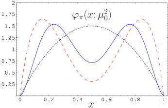
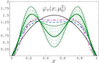
Figure 1: (a) Profiles of pion DAs normalized at $\mu_{0}^{2}=1~{}{\rm GeV}^{2}$: BMS model [1]—solid line; CZ model [12]—dashed line; asymptotic DA—dotted line. (b) BMS “bunch” [1] in comparison with $\varphi_{\text{as}}$, $\varphi_{\text{PR}}$ (dashed line) [13], $\varphi_{\text{Dor}}$ (dash-dotted line) [14].

3 Comparison with the CLEO data on the pion-photon transition

It was shown in [15] at LO and later extended [16] to NLO of QCD perturbation theory [17] that the light-cone QCD sum-rule method allows to perform all calculations in the $\gamma^{*}(Q^{2})\gamma(q^{2})\to\pi^{0}$ form factor for sufficiently large $q^{2}$ and analytically continue the results to the limit $q^{2}=0$, hence avoiding problems arising when a photon becomes real. Recently [2], we have revised and refined this sort of data processing accounting for a correct ERBL [11] evolution of the pion DA, including thresholds effects in the running coupling, estimating more accurately the contribution of the twist-4 contribution, and improving the error estimates in determining the $1\sigma$- and $2\sigma$-error contours. Avoiding here technical details, we gather the results of our analysis in Fig. 2. The predictions shown correspond to the following pion DA models with associated $\sigma$ deviations and designations for the form-factor predictions displayed in the right panel: $\varphi_{\rm CZ}$ (◼, $4\sigma$, upper dashed line) [12]; BMS-“nonlocal QCD SRs bunch” (shaded rectangle), $\varphi_{\rm BMS}$ (✖, $1\sigma$—left panel, shaded strip—right panel) [1]; three instanton-based models, viz., [18] (★, $3\sigma$, dotted line), [13] (✦, $2\sigma$, dash-dotted line), and [19] ($\blacktriangle$, $3\sigma$—only left panel); and the asymptotic pion DA $\varphi_{\rm as}$ (◆, $3\sigma$, lower dashed line). A recent transverse lattice result [20] (▼, $2\sigma$) is also shown—left panel only.

   

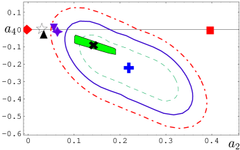
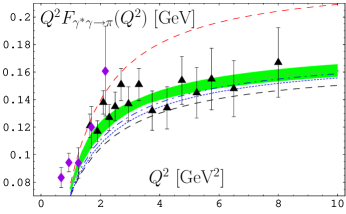
Figure 2: (a) $Q^{2}F_{\gamma^{*}\gamma\to\pi}(Q^{2})$ CLEO-data analysis in terms of error contours in the ($a_{2}$,$a_{4}$) plane. The line assignments are: broken line—$1\sigma$; solid line—$2\sigma$; dash-dotted line—$3\sigma$. Various pion DAs are shown, evaluated at $\mu^{2}_{\rm SY}=5.76$ GeV² after NLO ERBL evolution.. The slanted shaded rectangle represents the nonlocal QCD sum-rule constraints on ($a_{2},~{}a_{4}$) [1] for $\lambda^{2}_{\rm q}=0.4$ GeV². (b) Light-cone sum-rule predictions for $Q^{2}F_{\gamma^{*}\gamma\to\pi}(Q^{2})$ in comparison with the CELLO (diamonds, [21]) and the CLEO (triangles, [4]) data evaluated with $\delta_{\rm Tw-4}^{2}=0.19$ GeV² [2].

To summarize, the main results obtained in [2] are: (i) Both DAs, $\varphi_{\pi}^{\rm as}$ [11] and $\varphi_{\pi}^{\rm CZ}$ [12] are disfavored by the CLEO data at $3\sigma$ and $4\sigma$, respectively. In contrast, $\varphi_{\pi}^{\rm BMS}$ lies within the $1\sigma$-error ellipse. Model DAs from instanton-based approaches [13, 14, 18, 19] are close to but still outside the $2\sigma$ region. (ii) The extracted coefficients $a_{2}$ and $a_{4}$ are rather sensitive to the strong radiative corrections and the size of the twist-4 contribution. (iii) The value of the vacuum nonlocality extracted from the CLEO data is $\lambda_{\rm q}^{2}\lesssim 0.4$ GeV². Turning to the form-factor predictions, one observes from Fig. 2 (Right) that the BMS “bunch” of pion DAs is in good agreement with the CLEO data [4] but also with the CELLO data [21], while the behavior of rival DAs reflects the situation shown in the left panel: the prediction from the CZ model overshoots the data considerably, while that from $\varphi_{\pi}^{\rm as}$—and DAs close to it—are underestimating both sets of experimental data.

4 Electromagnetic pion form factor. Theory and phenomenology

The crucial new elements of the calculation below are: (i) use of the BMS pion DA, (ii) application of two-loop Analytic Perturbation Theory (APT), and (iii) a more accurate way, based on local duality, to join the soft part with the hard form-factor contribution.

The pion’s electromagnetic form factor can be generically written as [11] $F_{\pi}(Q^{2})=F_{\pi}^{\rm Fact}(Q^{2})+F_{\pi}^{\rm non-Fact}(Q^{2}),$ where $F_{\pi}^{\rm Fact}(Q^{2})$ is the factorized part within pQCD and $F_{\pi}^{\rm non-Fact}(Q^{2})$ is the “soft” part containing subleading power-behaved (e.g., twist-4) contributions originating from nonperturbative effects. The leading-twist factorizable contribution can be expressed as a convolution in the form $F_{\pi}^{\rm Fact}(Q^{2};\mu_{\rm R}^{2})=f_{\pi}^{2}\varphi_{\pi}^{*}(x,\mu_{\rm F}^{2})\otimes T_{\rm H}(x,y,Q^{2};\mu_{\rm F}^{2},\mu_{\rm R}^{2})\otimes\varphi_{\pi}(y,\mu_{\rm F}^{2})$, where $\mu_{\rm F}$ is the factorization scale between the long- and short-distance dynamics, $\mu_{\rm R}$ stands for the renormalization scale. The hard-scattering amplitude, $T_{\rm H}(x,y,Q^{2};\mu_{\rm F}^{2},\mu_{\rm R}^{2})$, describing short-distance interactions at the parton level, has been evaluated to NLO accuracy ([22] and references cited therein) using the terminology introduced in [9] to which we refer for details. Then, one obtains $F_{\pi}^{\rm Fact}(Q^{2};\mu_{\rm R}^{2})=F_{\pi}^{\rm LO}(Q^{2};\mu_{\rm R}^{2})+F_{\pi}^{\rm NLO}(Q^{2};\mu_{\rm R}^{2})$, where the LO and NLO terms read, respectively,

$$F_{\pi}^{\rm LO}(Q^{2};\mu_{\rm R}^{2}) = \alpha_{\rm s}(\mu_{\rm R}^{2})\,{\cal F}_{\pi}^{\rm LO}(Q^{2})$$ (3)

$$Q^{2}{\cal F}_{\pi}^{\rm LO}(Q^{2}) \equiv 8\,\pi\,f_{\pi}^{2}\,\left[1+a_{2}^{\rm D,NLO}(Q^{2})+a_{4}^{\rm D,NLO}(Q^{2})\right]^{2}\,,$$ (4)

$$F_{\pi}^{\rm NLO}(Q^{2};\mu_{\rm R}^{2})=\frac{\alpha_{\rm s}^{2}(\mu_{\rm R}^{2})}{\pi}\,\left[{\cal F}_{\pi}^{\rm D,NLO}(Q^{2};\mu_{\rm R}^{2})+{\cal F}_{\pi}^{\rm ND,NLO}(Q^{2};N_{\rm Max}=\infty)\,\right].$$ (5)

Here $N_{\rm Max}$ marks the maximal number of Gegenbauer harmonics taken into account and the calligraphic designation denotes quantities with their $\alpha_{\rm s}$-dependence pulled out. Note that because we take into account the NLO evolution of the pion DA, the displayed terms contain diagonal (D) as well as (the NLO term) non-diagonal (ND) components. The effects of the LO DA evolution are crucial [22], while the NLO ones are relatively of less importance. Hence, we set here: $a_{n}^{\rm D,NLO}\to a_{n}^{\rm D,LO}\;\,\mbox{and}\;\,a_{n}^{\rm ND,NLO}\to 0.\,$ Studying $F_{\pi}$ beyond the LO requires an optimal renormalization scheme and scale setting in order to minimize the influence of higher-order loop corrections (see [9] for a fully fledged discussion). To join the hard with the soft contribution (the latter being calculated with the aid of local duality (LD), we have to correct the low-$Q^{2}$ behavior of the factorizable part to fulfill the Ward identity at $Q^{2}=0$, i.e., $F_{\pi}(Q^{2};\mu_{\rm R}^{2})=F_{\pi}^{\rm LD}(Q^{2})+F_{\pi}^{\rm Fact-WI}(Q^{2};\mu_{\rm R}^{2})\,$ with $F_{\pi}^{\rm Fact-WI}(Q^{2};\mu_{\rm R}^{2})=Q^{4}/\left(2s_{0}^{\rm 2-loop}+Q^{2}\right)^{2}F_{\pi}^{\rm Fact}(Q^{2};\mu_{\rm R}^{2}).$

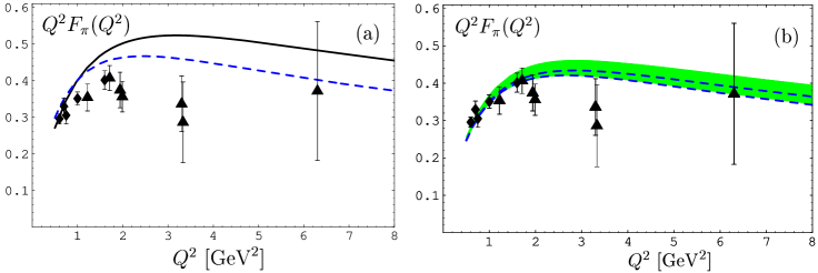
Figure 3: (a) Predictions for $Q^{2}F_{\pi}(Q^{2})$ obtained with the BMS pion DA using standard pQCD within the $\overline{{\rm MS}}$ scheme and adopting $\mu_{\rm R}^{2}=Q^{2}$ (dashed line). The solid line corresponds to the $\overline{\text{BLM}}$ scale setting introduced in [9]. The experimental data are taken from [23] (diamonds) and [24] (triangles). (b) Prediction for $Q^{2}F_{\pi}(Q^{2})$ calculated with the “Maximally Analytic ” procedure and with the BMS “bunch” of pion DAs.

The next step is to apply for the calculation of $F_{\pi}^{\rm Fact}(Q^{2})$ APT. This is done by employing two different analytization procedures: (i) A Maximally Analytic prescription [9], meaning that analyticity has been imposed not only on the coupling, but also on its powers, which, therefore, have their own dispersive images. This amounts to

$$\left[F_{\pi}^{\rm Fact}(Q^{2};\mu_{\rm R}^{2})\right]_{\rm MaxAn}\ =\bar{\alpha}_{\rm s}^{(2)}(\mu_{\rm R}^{2})\,{\cal F}_{\pi}^{\rm LO}(Q^{2})+\frac{1}{\pi}\,{\cal A}_{2}^{(2)}(\mu_{\rm R}^{2})\,{\cal F}_{\pi}^{\rm NLO}(Q^{2};\mu_{\rm R}^{2})\,,$$ (6)

where $\bar{\alpha}_{\rm s}^{(2)}(\mu_{\rm R}^{2})$ is the two-loop analytic coupling and ${\cal A}_{2}^{(2)}(\mu_{\rm R}^{2})$ the analytic version of its second power in two-loop order [9]. (ii) Another procedure, we call [9] Naive Analytic, replaces in $F_{\pi}^{\rm Fact}$ the strong coupling and its powers by the analytic coupling $\bar{\alpha}_{\rm s}$ and its powers $\left[\bar{\alpha}_{\rm s}^{(2)}(\mu_{\rm R}^{2})\right]^{2}$, entailing the requirement [10]

$$\left[F_{\pi}^{\rm Fact}(Q^{2};\mu_{\rm R}^{2})\right]_{\rm NaivAn}\ =\bar{\alpha}_{\rm s}^{(2)}(\mu_{\rm R}^{2})\,{\cal F}_{\pi}^{\rm LO}(Q^{2})+\frac{1}{\pi}\,\left[\bar{\alpha}_{\rm s}^{(2)}(\mu_{\rm R}^{2})\right]^{2}\,{\cal F}_{\pi}^{\rm NLO}(Q^{2};\mu_{\rm R}^{2})\,.$$ (7)

The results for $F_{\pi}$ vs. the experimental data are displayed in Fig. 3(b) and Fig. 4.

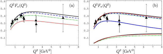
Figure 4: Predictions for $Q^{2}F_{\pi}(Q^{2})$ using APT and the BMS DA in conjunction with the “Naive Analytic” (a) and “Maximally Analytic” (b) procedures: $\overline{\text{MS}}$ scheme and $\mu_{\rm R}^{2}=Q^{2}$ (dashed line); BLM (dotted line); $\overline{{\rm BLM}}$ (solid line); $\alpha_{V}$-scheme (dash-dotted line). The single solid line in panel (b) shows the prediction for the soft form-factor part; below this, the corresponding hard contributions are displayed.

5 Summary and conclusions

The BMS pion DAs [1] successfully pass the comparison with the CLEO data [4] at the $1\sigma$ level, as highlighted in Fig. 2 (conforming also with the CELLO data [21]). Employing 2-loop APT—naive and maximal— we have calculated the hard part of the electromagnetic pion form factor within various renormalization schemes and using different scale settings. Joining the hard part with the soft one on the basis of local duality, we have derived predictions that reproduce the available data rather well, especially using the “Maximally Analytic” procedure (Fig. 3(b)). Moreover, we found that this procedure minimizes the influence of scheme and scale-setting ambiguities on the form-factor predictions.

References

- [1] A.P. Bakulev, S.V. Mikhailov and N.G. Stefanis, Phys. Lett. B508 (2001) 279.
- [2] A.P. Bakulev, S.V. Mikhailov and N.G. Stefanis, Phys. Rev. D 67 (2003) 074012; Phys. Lett. B578 (2004) 91; hep-ph/0310267; hep-ph/0312141.
- [3] S.V. Mikhailov and A.V. Radyushkin, JETP Lett. 43 (1986) 712; Sov. J. Nucl. Phys. 49 (1989) 494; Phys. Rev. D 45 (1992) 1754; A.P. Bakulev and A.V. Radyushkin, Phys. Lett. B271 (1991) 223; S.V. Mikhailov, Phys. Atom. Nucl. 56 (1993) 650.
- [4] J. Gronberg et al., Phys. Rev. D 57 (1998) 33.
- [5] A.P. Bakulev and S.V. Mikhailov, Phys. Rev. D 65 (2002) 114511.
- [6] D.V. Shirkov and I.L. Solovtsov, Phys. Rev. Lett. 79 (1997) 1209.
- [7] D.V. Shirkov, Theor. Math. Phys. 127 (2001) 409; Eur. Phys. J. C22 (2001) 331; D.V. Shirkov and I.L. Solovtsov, Phys. Part. Nucl. 32S1 (2001) 48.
- [8] A.I. Karanikas and N.G. Stefanis, Phys. Lett. B504 (2001) 225; N.G. Stefanis, Lect. Notes Phys. 616 (2003) 153.
- [9] A.P. Bakulev, K. Passek-Kumerički, W. Schroers and N.G. Stefanis, Phys. Rev. D 70 (2004) 033014.
- [10] N.G. Stefanis, W. Schroers and H.C. Kim, Phys. Lett. B449 (1999) 299; Eur. Phys. J. C18 (2000) 137.
- [11] A.V. Efremov and A.V. Radyushkin, Phys. Lett. B94 (1980) 245; Theor. Math. Phys. 42 (1980) 97; G.P. Lepage and S.J. Brodsky, Phys. Rev. D 22 (1980) 2157.
- [12] V.L. Chernyak and A.R. Zhitnitsky, Phys. Rep. 112 (1984) 173.
- [13] M. Praszalowicz and A. Rostworowski, Phys. Rev. D 64 (2001) 074003.
- [14] A.E. Dorokhov, JETP Lett. 77 (2003) 63.
- [15] A. Khodjamirian, Eur. Phys. J. C6 (1999) 477.
- [16] A. Schmedding and O.I. Yakovlev, Phys. Rev. D 62 (2000) 116002.
- [17] F. del Aguila and M.K. Chase, Nucl. Phys. B193 (1981) 517; E.P. Kadantseva, S.V. Mikhailov, and A.V. Radyushkin, Sov. J. Nucl. Phys. 44 (1986) 326.
- [18] V.Y. Petrov et al., Phys. Rev. D 59 (1999) 114018.
- [19] I.V. Anikin, A.E. Dorokhov and L. Tomio, Phys. Part. Nucl. 31 (2000) 509.
- [20] S. Dalley and B. van de Sande, Phys. Rev. D 67 (2003) 114507.
- [21] H.J. Behrend et al. [CELLO Collaboration], Z. Phys. C49 401 (1991) 401.
- [22] B. Melić, B. Nižić and K. Passek, Phys. Rev. D 60 (1999) 074004.
- [23] J. Volmer et al., Phys. Rev. Lett. 86 (2001) 1713.
- [24] C.N. Brown et al., Phys. Rev. D 8 (1973) 92; C.J. Bebek et al., D 13 (1976) 25.