SLAC-PUB-10701

hep-ph/0409127

D-Terms, Unification, and the Higgs Mass
Alexander Maloney^1,2, Aaron Pierce^1,2, Jay G. Wacker²

1. Theory Group

Stanford Linear Accelerator Center

Menlo Park, CA 94025

2. Institute for Theoretical Physics

Stanford University

Stanford, CA 94305

We study gauge extensions of the MSSM that contain non-decoupling $D$-terms, which contribute to the Higgs boson mass. These models naturally maintain gauge coupling unification and raise the Higgs mass without fine-tuning. Unification constrains the structure of the gauge extensions, limiting the Higgs mass in these models to $m_{h}\,\raise 1.29167pt\hbox{$<$\kern-7.5pt\lower 4.30554pt\hbox{$\sim$}}\,\mbox{150 $\text{ GeV}$}$. The $D$-terms contribute to the Higgs mass only if the extended gauge symmetry is broken at energies of a few TeV, leading to new heavy gauge bosons in this mass range.

1 Introduction

The Minimal Supersymmetric Standard Model (MSSM) makes a firm prediction for the mass of the lightest Higgs boson. Supersymmetry (SUSY) relates the quartic coupling of the Higgs boson to the Standard Model (SM) gauge couplings, resulting in a tree-level prediction for the Higgs mass: $m_{h}<M_{Z}=91$ GeV. The current Higgs mass bound from LEP II ($m_{h}\geq 114.4\text{ GeV}$ [1]) can be accommodated, but only if the parameters are somewhat fine-tuned — proponents of the MSSM would have been more comfortable had the Higgs boson been discovered closer to the tree-level prediction. (See [2] for a discussion of fine-tuning in the MSSM.) The alternative to fine-tuning is new physics at the TeV scale that contributes to the Higgs mass. For recent attempts, see [3, 4, 5, 6, 7].

There are two hints as to the nature of this new TeV scale physics. The first is the striking unification of the gauge couplings in the MSSM [8]. We will demand that any modifications to the Higgs sector maintain unification. Second, the theory be should as natural as possible; some mechanisms raise the Higgs boson mass only by introducing a substantial fine-tuning. As we will discuss in section 2.1, these two criteria lead us to study particular gauge extensions of the MSSM. In these extensions the Higgs mass is increased through non-decoupling $D$-terms [3, 9]. To have a significant effect, the new gauge group under which the Higgs is charged must have a large coupling.

Unfortunately, the simplest gauge extensions of the MSSM spoil gauge coupling unification. In these cases, the only recourse is to include additional particles whose sole purpose to restore unification, “unifons.” In this paper, using the success of the MSSM as a guide, we will describe two models without these designer particles. In these models, gauge coupling unification constrains the size of the non-decoupling $D$-terms, limiting the potential increase in the Higgs mass. This is easy to see: in our approach, we mix the electroweak $SU(2)\times U(1)$ with additional gauge groups. This increases the $SU(2)\times U(1)$ gauge couplings, which are related to the Higgs quartic coupling by supersymmetry. Unification relates these new electroweak gauge groups to a new colored gauge group, which is in danger of becoming strongly coupled. This puts an upper bound on the size of the $SU(2)\times U(1)$ coupling, and therefore on the $D$-term contribution to the Higgs mass.

In Sec. 2 we present two gauge extensions of the MSSM that naturally maintain unification, and can contribute to the Higgs mass without invoking fine tuning. The first model adds an extra copy of a GUT gauge group, which is coupled to the standard model gauge content by bi-fundamentals. We call this approach “product unification.” The second model is one of accelerated unification [10], where the additional gauge content is a copy of the standard model gauge group. In this case unification is maintained, but occurs at a much lower scale. Notably, this model requires the presence of a second pair of Higgs doublets at low energy, which might seem an ad hoc addition to the model, resurrecting the “unifon” specter. On the contrary, we will argue in Sec. 5.3 that their existence can be related to the observed stability of the proton via a missing-partner mechanism [11].

The organization of the rest of the paper is as follows. In Sec. 3 we discuss in detail non-decoupling $D$-terms, focusing on the specific potential that arises in both of the models described above. In Sec. 4 we apply these results to the product unification model and discuss implications for the Higgs mass. We find that in this case the non-decoupling $D$-terms can contribute roughly 10 GeV to the Higgs mass. In Sec. 5 we turn to the minimal accelerated unification model, and conclude that $D$-terms can easily raise the Higgs mass by $30-40$ GeV. We discuss precision unification in both cases. Finally we conclude and present an outlook for these two models.

2 Motivation: The Higgs Mass in Unified Models

In Sec. 2.1, we will begin by outlining various modifications to the MSSM that can raise the Higgs mass. Of these, we will argue that only two – the NMSSM [12] and non-decoupling $D$-terms – can accommodate unification without fine tuning. We will focus on the second of these, and give in Sec. 2.2 a more detailed description of the restrictions that unification places on this approach. There are two distinct possibilities: the unification scale may be preserved by the new gauge structure, or it may be lowered. In Sec. 2.3 we briefly describe the two simplest implementations of these alternatives. The first involves adding an extra unified gauge group, while the second requires the addition of a copy of the standard model gauge content.

2.1 Increasing the Higgs Mass

We will now discuss various ways of raising the Higgs mass in supersymmetric models, and conclude that gauge extensions and the NMSSM are the two most attractive alternatives.

SUSY Breaking in the MSSM

The simplest way to increase the Higgs mass requires no new physics; it simply uses the SUSY breaking effects associated with the top squark [13]. In general, a Yukawa interaction between the Higgs and some other particle will contribute both to the (mass)² of the Higgs boson and to its quartic coupling, as

$$\delta\lambda=\frac{N_{c}y^{4}}{8\pi^{2}}\left(\log\frac{m_{\text{B}}}{m_{\text{F}}}+a^{2}\left(1-\frac{a^{2}}{12}\right)\right),\hskip 36.135pt\delta m^{2}=-\frac{N_{c}(1+a^{2})y^{2}}{8\pi^{2}}\left(m^{2}_{\text{B}}-m^{2}_{\text{F}}\right)\log\Lambda^{2}.$$ (1)

Here $N_{c}$ is the number of colors, $m_{B}$ and $m_{F}$ are the boson and fermion masses, and we have included the SUSY violating $A$-term

$$\mathcal{L}_{\text{soft}}\supset y\,a\,m_{B}\;h\tilde{f}\tilde{f}^{c}.$$ (2)

At loop level, these effects give a logarithmically divergent contribution to the Higgs boson (mass)², but only a finite contribution to the Higgs quartic coupling. The result is fine-tuning, making this mechanism rather unattractive. For example, every 10 GeV increase in the Higgs mass above 115 GeV requires a doubling of the top squark mass.

We could use the $A$-term to improve this situation, but such contributions are typically small. The $A$-term contribution is maximized at $a=\sqrt{6}$, a parameter choice that has been dubbed “maximal mixing.” SUSY breaking scenarios often have much smaller $A$-terms, reducing potential contributions to the Higgs mass. For example, as $a$ decreases from $\sqrt{6}$ to $1$ the contribution to $\delta\lambda$ decreases by a factor of 3. Moreover, radiative corrections from $A$-terms increase fine tuning in the MSSM. We therefore conclude that $A$-terms are not useful for raising the Higgs mass.

Additional Matter

It is possible to add Yukawa interactions to new particles, but precision electroweak constraints make this unlikely. Chiral multiplets that get their masses from electroweak symmetry breaking are very strongly constrained. Vector-like matter makes the already modest SUSY-breaking logarithm in Eq. (1) even smaller, so is not a useful alternative.

New $F$-Terms

A more attractive way of raising the Higgs mass is to add new fields that directly couple to $h_{u}$ or $h_{d}$ in the superpotential. At the renormalizable level the only possibilities are a gauge singlet, $n$, and an SU(2) triplet, $T$. The possible superpotential terms are

$$W=\left(\begin{array}[]{cc}h_{u}&h_{d}\end{array}\right)\left(\begin{array}[]{cc}\kappa_{+}T_{+}&\kappa_{n}n+\kappa_{0}T_{0}\\ \kappa_{n}n+\kappa_{0}T_{0}&\kappa_{-}T_{-}\end{array}\right)\left(\begin{array}[]{c}h_{u}\\ h_{d}\end{array}\right),$$ (8)

where we have included three different triplets $T_{\pm},T_{0}$ with hypercharges $\pm 1$, $0$. These interactions contribute to the quartic coupling of the Higgs bosons at the tree-level, so can raise the Higgs mass without fine-tuning [14]. However, the triplets will disturb gauge coupling unification unless additional matter is added to fill out an SU(5) multiplet. The smallest such multiplets are the 24 of SU(5) for $T_{0}$, and the 15+$\mathbf{\overline{15}}$ for $T_{\pm}$. Absent an obvious rationale for adding the remainder of the GUT multiplets, we find this possibility somewhat distasteful. Moreover, the addition of so much matter raises the prospect of a Landau pole. Finally, if the triplets acquire a small vacuum expectation value (vev), they can have dangerous contributions to the $T$ parameter. On the other hand, the presence of a singlet $n$ will not affect the unification of couplings at the one-loop level, making it a more promising candidate. This coupling has a positive beta function and will lead to a Landau pole at large coupling. This constrains the size of the $nh_{u}h_{d}$ coupling at the weak scale, thus limiting its contribution to the Higgs mass [15].

New $D$-Terms

Finally, one can introduce new gauge groups. The associated $D$-terms will then contribute to the Higgs quartic coupling. In the SUSY limit, these new contributions exactly decouple when the gauge groups break down to the MSSM. On the other hand, if the scale of SUSY breaking is close to the scale of the breaking of the gauge groups, there are non-decoupling $D$-terms which can raise the Higgs mass – essentially, when integrated out these terms introduce hard SUSY breaking into the MSSM [3].

These contributions to the quartic coupling (and hence the physical Higgs boson mass) arise at tree level, while contributions to the (mass)² occur only at loop level. This allows an increase in the Higgs boson mass without significant fine-tuning. However, this new non-supersymmetric quartic coupling generates a quadratic divergence in the Higgs mass, which is cut off at the mass of the new vector bosons. To prevent fine tuning, we therefore require that this contribution not be too large, since

$$\frac{\delta\lambda}{\lambda+\delta\lambda}\frac{M_{V}^{2}}{16\pi^{2}v^{2}}\approx\text{Fine Tuning}^{-1}.$$ (9)

This constrains the breaking scale to be in the 3 – 10 TeV range. The lower limit is set by precision electroweak considerations.

We have seen that non-decoupling $D$-Terms have the potential to raise the Higgs mass without fine-tuning, but we must still require that the new fields do not upset unification. We will now proceed to outline the two different ways that extended gauge sectors can accomplish this, and present two minimal implementations of this mechanism.

2.2 Unification in the MSSM

At one loop, gauge coupling unification can be tested by examining the following relation between the inverse gauge couplings and the one loop beta functions for the gauge groups:

$$\frac{\alpha^{-1}_{3}(M_{Z^{0}})-\alpha^{-1}_{2}(M_{Z^{0}})}{\alpha^{-1}_{2}(M_{Z^{0}})-\alpha^{-1}_{1}(M_{Z^{0}})}=\frac{b_{3}-b_{2}}{b_{2}-b_{1}}\equiv B^{32}_{21},$$ (10)

where $b_{i}$ are the one loop beta function coefficients. Using the experimentally measured values of the gauge couplings at the weak scale [16],

$$\begin{array}[]{lll}\alpha_{EM}^{-1}(M_{Z^{0}})&=&127.918\pm 0.018\\ \sin^{2}\theta_{W}(M_{Z^{0}})&=&0.23120\pm 0.00015\\ \alpha_{s}(M_{Z^{0}})&=&0.1187\pm 0.0020\end{array}$$ (11)

the left hand side of Eq. (10) is $0.719\pm 0.004$. In the MSSM, we have $(b_{1},b_{2},b_{3})=(33/5,1,-3)$, so $B^{32}_{21}=0.714$. This agreement summarizes the success of gauge coupling unification in the MSSM at one-loop.

We must now ask what mechanisms allow us to raise the Higgs mass without changing $B^{32}_{21}$. One possibility is to add extra matter only in complete GUT multiplets. Then all the $b_{i}$ are all shifted by a fixed amount – in this case the unification scale is unchanged, but the value of the gauge couplings at unification may be altered. The NMSSM is a trivial implementation of this strategy (all $b_{i}$ are unchanged), and, as described above, is effective in raising the Higgs mass. If we wish to consider gauge extensions to the MSSM, we must add a complete unified gauge group to the model. A model of this form, which we refer to as product unification, will be described in the next subsection, and in greater detail in Sec. 4.

The other natural possibility that keeps $B^{23}_{12}$ unchanged is to add matter in such a way that the $b_{3}-b_{2}$ is changed, but a proportional change is made in $b_{2}-b_{1}$. In this case unification still occurs, but at a lower scale. A specific implementation of this idea is accelerated unification [10], where the unification scale is brought down to the intermediate scale. The extra gauge content is simply another copy of $SU(3)\times SU(2)\times U(1)$. A model of this form will be described below, and in more detail in Sec. 5.

2.3 Two Minimal Gauge Extensions of the MSSM

We will present two minimal models that contain non-decoupling $D$-terms and preserve unification. Product unification adds a full GUT gauge group; accelerated unification adds a second copy of the MSSM gauge group.

Both of these are closely related to deconstructed dimensions [17]. The first model, product unification, is equivalent to having an extra dimensional GUT with $SU(3)\times SU(2)\times U(1)$ gauged on the boundary. The second model is equivalent to a bulk $SU(3)\times SU(2)\times U(1)$ gauge theory with power-law “unification” at a low scale. In order to have non-decoupling $D$-terms the effective radius must be 1 – 10 TeV, meaning that the bulk of the running occurs above the naive five dimensional cut-off. In both examples we will consider the minimally deconstructed theories, which we now describe.

2.3.1 Product Unification

In this approach, the high energy gauge group is $G=SU(3)\times SU(2)\times U(1)$, augmented by a grand unified gauge group, $G_{GUT}$. Near the TeV scale, the product $G\times G_{GUT}$ is broken down to the standard model gauge group, $G_{SM}$ (See Fig. 1). The matter and Higgs fields of the standard model are charged under $G$. After the breaking, they inherit the usual standard model quantum numbers.

Figure 1: A minimal model of product unification. The extended gauge group breaks down to the diagonal subgroup (the SM gauge group) at the TeV scale.

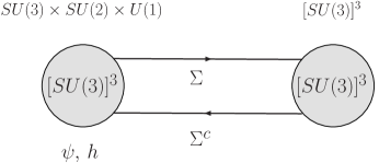
Figure 2: A theory space diagram of the product unification model discussed in the text. In addition to the usual $SU(3)\times SU(2)\times U(1)$, there is an $SU(3)^{3}$ gauge group. The $\Sigma,\Sigma^{c}$ fields are bi-fundamentals connecting these groups. The three generations of matter, denoted $\psi$, and the pair of Higgs doublets, $h$, are charged under $SU(3)\times SU(2)\times U(1)$. We consider a model where $SU(3)\times SU(2)\times U(1)$ unifies into the trinified group $SU(3)^{3}$ at the GUT scale.

The breaking to the MSSM occurs when link fields, $\Sigma$ and $\Sigma^{c}$, acquire a vev. These fields transform as bi-fundamentals of the global symmetry associated with the GUT gauge group. The structure of this model is similar to that of minimal deconstructed gaugino mediation [18]; however, we will remain agnostic about the exact mechanism of supersymmetry breaking.

While any GUT representation for the link fields will leave unification undisturbed, here we take the fields to transform under a trinified [20] representation (See Fig. 2). The reasons are two–fold. First, this representation is the smallest possible. In trinification, the $\Sigma$ fields fall into representations of $SU(3)$ that only contribute $\Delta b=3$ to each beta function. In $SU(5)$ and $SO(10)$ unification, the link fields add 5 and 10 to $\Delta b$, respectively. Thus trinification contributes the least possible amount to the gauge coupling beta functions, which helps keep the theory perturbative. Second, this model is closely related to the minimal accelerated unification model, which we now discuss.

2.3.2 Accelerated Unification

In accelerated unification models [10], the Standard Model gauge group, $G_{\text{SM}}$, is the remnant of an enlarged group, $G_{\text{SM}}^{\mathcal{N}}$, that breaks to the diagonal subgroup at the TeV scale. The presence of extra matter changes the gauge coupling beta functions, causing the theories to unify at a much lower scale (see Fig. 3).

Figure 3: The minimal accelerated unification model, with $\mathcal{N}=2$, where two copies of the MSSM gauge group break down to the diagonal subgroup at the TeV scale.

The gauge and matter content of the $\mathcal{N}=2$ trinified model is summarized in Fig. 4. There are two copies of the low energy gauge group, which we denote $[SU(3)_{C}\times SU(2)_{L}\times U(1)_{Y}]_{A,B}$. The matter and Higgs bosons of the MSSM, as well as a new pair of Higgs bosons, are charged under $[SU(3)_{C}\times SU(2)_{L}\times U(1)_{Y}]_{A}$. Again, a vector-like pair of link fields, $\Sigma$ and $\Sigma^{c}$, is responsible for breaking the gauge groups down to the diagonal subgroup. These fields should form complete GUT multiplets, so as to not contribute to the relative running of the gauge couplings. A similar situation occurs in theories of gauge mediated supersymmetry breaking, where additional complete multiplets are used so as not to spoil unification. Because these fields make up full GUT multiplets, rather than the minimum necessary for the breaking of the gauge symmetry, some components of the $\Sigma$ fields can become pseudo-Goldstone bosons (PGBs). These particles can have important phenomenological consequences, which we will address in Sec. 5.

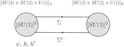
Figure 4: A theory space diagram of Minimal Accelerated Trinification. There are two copies of $SU(3)\times SU(2)\times U(1)$, labeled by subscripts $A$ and $B$, each of which unifies into $SU(3)^{3}$. The $\Sigma,\Sigma^{c}$ fields are bi-fundamentals connecting these groups. The three generations of matter, denoted $\psi$, and two pairs of Higgs doublets ($h$, $h^{\prime}$) are also shown.

While accelerated unification can accommodate any GUT representation for the link fields, trinification is particularly elegant. $SU(5)$ and $SO(10)$ models contain gauge boson mediated dimension-six proton decay operators, now dangerous due to the lower GUT scale, which are difficult to remove in 4-$D$ GUT models. Moreover, the dynamics of the breaking $G_{SM}^{2}\to G_{SM}$ is simplifier in trinified models, since it is possible to stabilize the potential for $\Sigma$ in the $D$-flat directions by adding renormalizable terms to the superpotential. This is in contrast with the $SU(5)$ case, where there is only a $D$-term potential; no stabilizing superpotential can be added without additional matter [10]. Directions that are not $D$-flat would lead to fine-tuning. In addition, as already described above, trinification has the smallest representation for the $\Sigma$ fields, ameliorating Landau pole issues.

We must also choose $\mathcal{N}$, the number of copies of the MSSM gauge group. In principle we may add as many copies as desired, as long as $2\mathcal{N}$ Higgs doublets are added at the same time. But the expected threshold corrections to unification grow with $\mathcal{N}$, so at large $\mathcal{N}$ unification appears accidental. Moreover, the gauge couplings scale as $\sqrt{\mathcal{N}}g_{SM}$, so strong coupling problems can arise at large $\mathcal{N}$. For these reasons we focus on $\mathcal{N}=2$, where we expect to have the best control over unification.

Finally, the $\mathcal{N}=2$ trinified model presented here has an elegant mechanism to prevent proton decay. As noted above, this model includes an extra pair of Higgs doublets in addition to the usual pair present in supersymmetric models. We may then couple one pair of Higgs doublets to the leptons and the other to the quarks, which suppresses baryon number violating interactions. We will discuss this mechanism in more detail in Sec. 5.3.2.

3 Non-Decoupling D-Terms

In this section we discuss the breaking of the extended gauge sector down to the SM gauge group. The breaking is essentially identical for the product and accelerated unification models, and will ultimately be the source of the non-decoupling $D$-Terms that raise the Higgs mass.

Breaking occurs when the link fields $\Sigma,\Sigma^{c}$ get a vev. In both of the models described above, the link fields can be organized into global $[SU(3)^{3}]_{A,B}$ multiplets as

$$\Sigma_{C}\sim(\mathbf{3}_{CA},\overline{\mathbf{3}}_{CB})\hskip 28.90755pt\Sigma_{C}^{c}\sim(\mathbf{3}_{CB},\overline{\mathbf{3}}_{CA})$$

$$\Sigma_{L}\sim(\mathbf{3}_{LA},\overline{\mathbf{3}}_{LB})\hskip 31.79897pt\Sigma_{L}^{c}\sim(\mathbf{3}_{LB},\overline{\mathbf{3}}_{LA})$$

$$\Sigma_{R}\sim(\mathbf{3}_{RA},\overline{\mathbf{3}}_{RB})\hskip 29.63095pt\Sigma_{R}^{c}\sim(\mathbf{3}_{RB},\overline{\mathbf{3}}_{RA}).$$ (12)

The hypercharge generator is given by

$$Y=-\frac{1}{6}\,T^{8}_{L}-\frac{1}{3}\,\tilde{T}^{8}_{R},$$ (13)

with $T^{8}_{L}=\text{diag}(1,1,-2)$ and $\tilde{T}^{8}_{R}=\text{diag}(-2,1,1)$. These fields come in a complete GUT multiplet and do not disturb unification.

3.1 Decoupling the $D$-Terms

To give the $\Sigma$ fields a vev, we must include a potential $V(\Sigma)$. The most general $SU(3)$ symmetric superpotential is

$$W_{\Sigma}=\lambda(\det\Sigma+\det\Sigma^{c})+\mu\text{ Tr }\Sigma\Sigma^{c}.$$ (14)

There is one such potential for each of ${\Sigma_{C},\Sigma_{L},\Sigma_{R}}$. The Kahler term is

$$K=\text{ Tr }e^{g_{A}V_{A}}\Sigma e^{-g_{B}V_{B}}\Sigma^{\dagger}+\text{ Tr }e^{g_{B}V_{B}}\Sigma^{c}e^{-g_{A}V_{A}}\Sigma^{c}{}^{\dagger}.$$ (15)

This potential has two $D$-flat minima at:

$$\langle\Sigma\rangle=\langle\Sigma^{c}\rangle=0\hskip 28.90755pt\langle\Sigma\rangle=\langle\Sigma^{c}\rangle=-\frac{\mu}{\lambda}{\hbox to0.0pt{1\hss}\hskip 1.6pt\hbox{1}}\equiv f{\hbox to0.0pt{1\hss}\hskip 1.6pt\hbox{1}}.$$ (16)

We focus on the second solution, which breaks $SU(3)\times SU(3)\rightarrow SU(3)$. The small fluctuations around the vev can be grouped into four complex fields $S$, $\eta$, $\pi$ and $\phi$:

$$\Sigma = e^{\eta/\sqrt{6}f}\exp(c_{A}\pi/f)\Sigma_{0}\exp(c_{B}\pi/f)$$

$$\Sigma^{c} = e^{-\eta/\sqrt{6}f}\exp(-c_{B}\pi/f)\Sigma_{0}\exp(-c_{A}\pi/f)$$ (17)

$$\Sigma_{0} \equiv \Big{(}f+\frac{S}{\sqrt{6}}\Big{)}{\hbox to0.0pt{1\hss}\hskip 1.6pt\hbox{1}}+\phi,$$

where $c_{A,B}$ are normalization constants. $S$ is the fluctuation of the vev, while $\eta$ and $\pi$ are the Goldstone boson superfields for the broken global $U(3)$ symmetries. Only a subgroup of this $U(3)$ is gauged. The determinant superpotential breaks the $U(1)$ of this $U(3)$ explicitly, giving $\eta$ a mass. The fields transform under the unbroken $SU(3)$ as

$$S\sim\mathbf{1},\hskip 21.68121pt\phi\sim\mathbf{8},\hskip 21.68121pt\eta\sim\mathbf{1},\hskip 21.68121pt\pi\sim\mathbf{8}.$$ (18)

Expanding the superpotential around the vev, we find:

$$W=2\lambda\cosh\sqrt{\frac{3}{2}}\frac{\eta}{f}\det\Sigma_{0}+\mu\text{ Tr }\Sigma_{0}^{2}.$$ (19)

This yields masses

$$\mu_{S}=-\mu,\hskip 21.68121pt\mu_{\phi}=2\mu,\hskip 21.68121pt\mu_{\eta}=-3\mu,\hskip 21.68121pt\mu_{\pi}=0.\hskip 21.68121pt$$ (20)

The $D$-terms decouple in the supersymmetric limit. To see this, define the vector superfields $V_{0}$ and $V_{H}$ by

$$g_{A}V_{A}=g_{0}V_{0}-g_{0}\frac{g_{A}}{g_{B}}V_{H}\hskip 36.135ptg_{B}V_{B}=g_{0}V_{0}+g_{0}\frac{g_{B}}{g_{A}}V_{H},$$ (21)

with $g_{0}^{-2}=g_{A}^{-2}+g_{B}^{-2}$. It follows that $V_{H}$ acquires a mass while $V_{0}$ remains massless. Ignoring $V_{0}$, the Kahler term may be expanded to leading order as

$$K=2\text{ Tr }\phi^{\dagger}\phi+\Big{|}f+\frac{S}{\sqrt{6}}\Big{|}^{2}(6+\text{ Tr }|g_{H}V_{H}+(\pi+\pi^{\dagger})/f|^{2})+\eta^{\dagger}\eta+\cdots$$ (22)

where $g_{H}^{2}=g_{A}^{2}+g_{B}^{2}$. Using the gauge transformation $V\rightarrow V+\alpha+\alpha^{\dagger}$ we can go to unitary gauge, with $\pi=0$. Now consider a field, $H$, charged under $G_{A}$. The Kahler term contains the coupling to $V_{H}$ (for the moment we suppress the $e^{g_{0}V_{0}}$)

$$K=H^{\dagger}e^{g_{A}V_{A}}H=H^{\dagger}H-\frac{g_{0}g_{A}}{g_{B}}H^{\dagger}V_{H}H+\cdots$$ (23)

The superfield propagator at zero momentum in unitary gauge is given simply by $1/M_{V}^{2}$. So, integrating out $V_{H}$ gives

$$K_{\text{eff}}=H^{\dagger}H-\frac{g_{0}^{2}g_{A}^{2}}{g_{B}^{2}}\frac{1}{g_{H}^{2}f^{2}}|H^{\dagger}T^{a}H|^{2}+\cdots$$ (24)

The second term contains several interactions that provide important constraints on our models, but no scalar potential. The scalar potential comes from restoring the $e^{g_{0}V_{0}}$ to the first term. This is the just the standard decoupling of the $D$-terms, automatic in the superspace formalism. In component field language, this decoupling arises after integrating out the $C$-component (i.e. the lowest component) of $V_{H}$, which corresponds to the lowest component of $\pi+\pi^{\dagger}$ in unitary gauge.

3.2 Recoupling the $D$-Terms

To avoid decoupling and increase the Higgs mass, we must include SUSY breaking effects. In unitary gauge, this is accomplished by giving the lowest component of $V_{H}$ a supersymmetry breaking mass. This can be done in the superspace formalism with a $D$-term spurion

$$K=M_{V}^{2}(1+\theta^{4}m^{2}_{\text{soft}})\text{ Tr }V_{H}^{2},$$ (25)

with $M_{V}^{2}=g_{H}^{2}f^{2}$. Integrating out $V_{H}$, we find the effective Kahler potential for $H$

$$K_{\text{eff}}=H^{\dagger}e^{g_{0}V_{0}}H-\frac{g_{0}^{2}g_{A}^{2}}{g_{B}^{2}}\left(\frac{1}{g_{H}^{2}f^{2}}-\frac{m^{2}_{\text{soft}}\theta^{4}}{g_{H}^{2}f^{2}+m^{2}_{\text{soft}}}\right)|H^{\dagger}T^{a}H|^{2}+\cdots$$ (26)

where we have used the modified vector superfield propagator

$$\Delta_{F}(p,\theta,\bar{\theta})=-\frac{1}{p^{2}-M_{V}^{2}}+\frac{m^{2}_{\text{soft}}\theta^{4}}{p^{2}-(M_{V}^{2}+m^{2}_{\text{soft}})}+\cdots$$ (27)

In the limit $m^{2}_{\text{soft}}\rightarrow\infty$, the supersymmetry breaking coefficient in Eq. (26) is maximized, and the Higgs quartic coupling becomes (including the supersymmetric $D$-term from the unbroken gauge theory)

$$\lambda_{\text{Higgs}}=g_{0}^{2}\Big{(}1+\frac{g_{A}^{2}}{g_{B}^{2}}\Big{)}=g_{A}^{2}.$$ (28)

The quartic coupling is equal to the $D$-Term of the unbroken theory.

The $D$-term contributions the Higgs mass will be maximized if two conditions are satisfied. First, SUSY breaking must be effectively communicated to the vector boson mass from the soft Lagrangian. Second, the gauge coupling $g_{A}$ must be large. We will postpone the discussion of $g_{A}$ in specific models to Sec. 4.2 and 5.2, where we will see that unification restricts its size. Here we concentrate on how SUSY breaking is communicated to the vector boson soft mass. First, we write down the most general soft Lagrangian for $\Sigma$ using spurions

$$W = (1+a\theta^{2})\lambda(\det\Sigma+\det\Sigma^{c})+(1+b\theta^{2})\mu\text{ Tr }\Sigma\Sigma^{c}$$ (29)

$$K = (1+m^{2}\theta^{4})\left(\text{ Tr }e^{g_{A}V_{A}}\Sigma e^{-g_{B}V_{B}}\Sigma^{\dagger}+\text{ Tr }e^{g_{B}V_{B}}\Sigma^{c}e^{-g_{A}V_{A}}\Sigma^{c}{}^{\dagger}\right).$$ (30)

Rewriting in terms of the physical fields, we have

$$W = 2(1+a\theta^{2})\lambda\cosh\sqrt{\frac{3}{2}}\frac{\eta}{f}\det\Sigma_{0}+(1+b\theta^{2})\mu\text{ Tr }\Sigma_{0}^{2}$$ (31)

$$K = (1+m^{2}\theta^{4})\left(\text{ Tr }\phi^{\dagger}\phi+\Big{|}f+\frac{S}{\sqrt{6}}\Big{|}^{2}(6+g_{H}^{2}\text{ Tr }V_{H}^{2})+\frac{1}{2}(\eta^{\dagger}+\eta)^{2}+\cdots\right).$$ (32)

The lowest component of $V_{H}$ has already acquired a mass from $m^{2}$. In principle, the addition of SUSY breaking can induce a tadpole for $S$. This can be removed by a $\theta$ dependent shift. Such a shift can contribute to the vector mass (see Appendix B). For simplicity, we assume no tadpole is generated, which amounts to enforcing

$$m^{2}+b\mu-a\mu=0.$$ (33)

Relaxing this condition can lead to additional sources of non-decoupling, but this choice is sufficient to demonstrate that a significant non-decoupling is possible. Taking $a=0$ in Eq. (33), it follows that the masses of all the fields ($S$, $\phi$, $\eta$) are positive for $m^{2}>-\mu^{2}/2$. After integrating out the massive vector superfield the effective action is

$$K_{\text{eff}}=H^{\dagger}e^{g_{0}V_{0}}H+\frac{g_{0}^{2}g_{A}^{2}}{g_{B}^{2}}\frac{m^{2}\theta^{4}}{\left(\frac{g_{H}\mu}{\lambda}\right)^{2}+m^{2}}(H^{\dagger}T^{a}H)^{2}+\cdots$$ (34)

In fact, as long as $\lambda$ is not too small, $m^{2}\sim\mu^{2}\sim-b\mu$ gives $\mathcal{O}(1)$ re-coupling without destabilizing any modes.

4 Product Unification

We now return to a more detailed discussion of the model of Sec. 2.3.1. We begin with a discussion of one-loop running in this model, and derive the relations between low energy $SU(3)\times SU(2)\times U(1)$ parameters and the high energy $SU(3)^{3}$ parameters. We then address the central question of the Higgs mass in 4.2. We close this section with a discussion of unification beyond one-loop.

4.1 One Loop Running

This model unifies at one loop by construction. At one loop, the beta functions are

$$\frac{d}{dt}\frac{8\pi^{2}}{g^{2}_{i}(t)}=-b_{0,i}.$$ (35)

Here $i$ runs over the possible gauge groups, and the energy scale $t$ is defined to be $\log\left(\mu/3\text{ TeV}\right)$. The coefficients $b_{0,i}$ are listed in Table 1. The trinified gauge group $[SU(3)_{B}]^{3}$ starts at a unified coupling, and maintains unification under renormalization group (RG) flow. We denote this coupling $g_{B}$.

Using the standard MSSM beta functions, we can run the measured gauge couplings in Eq. (11) up to 3 TeV ($t=0$). There we match on to the extended gauge sector via

$$\frac{8\pi^{2}}{g^{2}_{i,{\text{SM}}}(0)}=\frac{8\pi^{2}}{g^{2}_{i,A}(0)}+\frac{8\pi^{2}}{g^{2}_{B}(0)}=\frac{8\pi^{2}}{g^{2}_{i,A}(t)}+b_{i,A}t+\frac{8\pi^{2}}{g^{2}_{B}(t)}+b_{B}t.$$ (36)

Unification is maintained in this extension because the same quantity (the last two terms in the above equation) is added to each of the SM gauge couplings. In Sec. 4.3 we will discuss higher order corrections to unification. Since the relative running of the gauge couplings is unaffected, the unification scale $t_{*}$ is unchanged: $t_{*}=29.5$, corresponding to the usual $E_{GUT}\sim 10^{16}\text{ GeV}$.

	$U(1)_{A}$	$SU(2)_{A}$	$SU(3)_{A}$	$[SU(3)_{B}]^{3}$
$V$	0	-6	-9	-9
$\psi$	6	6	6	0
$H$	$\frac{3}{5}$	1	0	0
$\Sigma$	3	3	3	3
$b_{0}$	$9\frac{3}{5}$	4	0	-6

Table 1: Beta function coefficients for the different gauge groups.

From Table 1, we see that the $SU(3)_{B}$ beta function coefficients are negative, so the corresponding couplings run strong at low energies. The requirement that $SU(3)_{B}$ remain perturbative above the TeV scale sets a maximum value for $g_{*,B}$, the value of the unified gauge coupling at $t_{*}$. If we define the low scale coupling $8\pi^{2}/g^{2}_{B}(0)=\Delta$, then

$$\frac{8\pi^{2}}{g^{2}_{*,B}}=\frac{8\pi^{2}}{g^{2}_{B}(0)}-b_{B}t_{*}=177+\Delta.$$ (37)

We require $\Delta$ to be reasonably large to ensure that $SU(3)_{B}$ stays weakly coupled.

Similarly, $8\pi^{2}/g^{2}_{*,A}$ can be obtained by matching the $A,B$ gauge couplings onto the measured gauge couplings at the weak scale,

$$\frac{8\pi^{2}}{g^{2}_{3}(0)}=64=\frac{8\pi^{2}}{g^{2}_{3,A}(0)}+\frac{8\pi^{2}}{g^{2}_{B}(0)}=\frac{8\pi^{2}}{g^{2}_{*,A}}+\frac{8\pi^{2}}{g^{2}_{*,B}}-(b_{3,A}+b_{B})t_{*}.$$ (38)

This implies that $8\pi^{2}/g^{2}_{*,A}=64-\Delta$. In Fig. 5 we plot the one loop running of the gauge couplings.

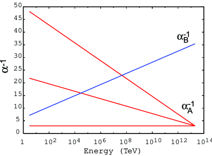
Figure 5: The running of the gauge couplings, with $\alpha_{A}^{-1}=3$ at the GUT scale.

4.2 The Higgs Mass

From Eq. (28) we see that the maximum fractional gain in the quartic depends on the gauge couplings. Making $g_{A}$ as large as possible, we find:

$$\frac{\delta\lambda_{SU(2)}}{\lambda_{SU(2)}}=\frac{g_{2,A}^{2}}{g_{2,{\text{SM}}}^{2}}-1\,\raise 1.29167pt\hbox{$<$\kern-7.5pt\lower 4.30554pt\hbox{$\sim$}}\,\frac{1}{3},\hskip 36.135pt\frac{\delta\lambda_{U(1)}}{\lambda_{U(1)}}=\frac{g_{1,A}^{2}}{g_{1,{\text{SM}}}^{2}}-1\,\raise 1.29167pt\hbox{$<$\kern-7.5pt\lower 4.30554pt\hbox{$\sim$}}\,\frac{1}{7}.$$ (39)

We have used the values of the gauge couplings computed in the previous section – higher loop corrections will be considered in in Sec. 4.3. The change in the quartic leads to a Higgs mass bound

$$m_{h^{0}}^{2}\leq\frac{(1.3g^{2}+1.15g^{\prime}{}^{2})}{g^{2}+g^{\prime}{}^{2}}M_{Z^{0}}^{2}=(102\text{ GeV})^{2},$$ (40)

a modest $11\text{ GeV}$ gain over the MSSM tree-level prediction. With top squarks of 400 GeV the Higgs mass can be lifted to the LEP II bound of 114 GeV. The fine-tuning of the MSSM may be ameliorated, but the Higgs cannot be made significantly heavier.

In this model $D$-term contributions to the Higgs mass are tightly constrained. This is because the value of $g_{2,A}(M_{Z^{0}})$ is bounded by the total amount of relative running between $SU(3)_{C}$ and $SU(2)_{L}$. This conclusion is fairly robust in any model with a product unification structure. Adding either more gauge groups or matter charged under $[SU(3)]^{3}_{B}$ will not effect the relative running between $SU(2)_{A}$ and $SU(3)_{A}$. One could charge some of the Standard Model matter (such as the first two generations) under $B$ gauge groups rather than $A$, but this would cause $SU(3)_{C,A}$ to run asymptotically free, tightening the bounds on $g_{A}(\Lambda)$. The only way to increase the Higgs mass bound, Eq. (40), is to charge the Higgs doublets under $[SU(3)]^{3}_{B}$. In this case, renormalizable Yukawa couplings are not possible, and some ad hoc change must be made to the $A$ sector to recover unification.

4.3 Precision Unification

While unification in this model is guaranteed at the one-loop level, several effects may alter the accuracy of this prediction, such as higher loop contributions, TeV scale supersymmetric threshold corrections, GUT scale threshold corrections, and SUSY breaking threshold corrections. The second two are model dependent, depending in detail upon the GUT scale physics, as well as the mechanism of supersymmetry breaking. The first two are, however, calculable. We now quantify the deviation from the one-loop prediction due to these effects.

Fortunately, the holomorphicity of gauge couplings in supersymmetric theories simplifies the analysis. At first, it might appear that unification is disturbed by splittings of the $\Sigma$ masses, which are induced by renormalization group evolution. This could lead to a TeV scale supersymmetric threshold correction. However, this correction cancels against certain two-loop contributions. The result is that higher loop effects can be encapsulated in the change in the anomalous dimensions of the light fields [22, 23].

Integrating the NSVZ exact beta function, we can derive an RG invariant matching equation (see Appendix A). We match the diagonal MSSM gauge coupling at the cutoff, $\Lambda$, and run down to low energies via

$$\frac{8\pi^{2}}{g^{2}(\mu)}+C_{2}\log g^{2}(\mu) = \frac{8\pi^{2}}{g_{A}^{2}(\Lambda)}+C_{2}\log g_{A}^{2}(\Lambda)+\frac{8\pi^{2}}{g_{B}^{2}(\Lambda)}+C_{2}^{B}\log g_{B}^{2}(\Lambda)$$ (41)

$$-C_{2}^{B}\log\frac{\Lambda^{2}}{\langle\Sigma\Sigma^{c}\rangle}+b_{\phi}\log\frac{\Lambda}{m_{\phi}}$$

$$+b_{0,\text{light}}\log\frac{\Lambda}{\mu}-\sum_{a}T_{2}(a)\log Z_{a}(\mu,\Lambda).$$

The sum is over the light fields of the MSSM, $C_{2}$ and $C_{2}^{B}$ are quadratic Casimirs, $b_{0,\text{light}}$ is the one-loop beta function of the light fields, and $b_{\phi}=3$ is the contribution of the $\phi$ fields to the beta function.

Our goal is to find the multi-loop analog of $B^{32}_{21}$, defined in Eq. (10). We start by considering the gauge couplings of the $SU(3)$ and $SU(2)$ sectors:

$$\Delta^{32}\equiv\frac{8\pi^{2}}{g_{3}^{2}(\mu)}-\frac{8\pi^{2}}{g_{2}^{2}(\mu)} = \Delta b^{32}_{\text{MSSM}}\log\frac{\Lambda}{\mu}+3\log\frac{g^{2}_{A}(\Lambda)}{g^{2}_{3}(\mu)}-2\log\frac{g^{2}_{A}(\Lambda)}{g^{2}_{2}(\mu)}+\delta z_{\psi}^{32}+\delta z_{h}^{32},$$ (42)

where $\Delta b^{32}_{\text{MSSM}}=-4$ is the difference between the one loop beta functions. The final terms come from the $\log Z$s of the light fields:

$$\delta z_{\psi}^{32}=\frac{1}{2}\log\prod_{f=1}^{3}\frac{Z_{u^{c}_{f}}Z_{d^{c}_{f}}}{Z_{q_{f}}Z_{l_{f}}},\hskip 28.90755pt\delta z_{h}^{32}=-\frac{1}{2}\log Z_{h_{u}}Z_{h_{d}},$$ (43)

all of which are evaluated from $\Lambda$ down to $\mu$. Similarly, for the $SU(2)$ and $U(1)$ couplings

$$\Delta^{21}\equiv\frac{8\pi^{2}}{g_{2}^{2}(\mu)}-\frac{8\pi^{2}}{g_{1}^{2}(\mu)} = \Delta b^{21}_{\text{MSSM}}\log\frac{\Lambda}{\mu}+2\log\frac{g^{2}_{A}(\Lambda)}{g^{2}_{2}(\mu)}+\delta z_{\psi}^{21}+\delta z_{h}^{21}$$ (44)

where $\Delta b^{21}_{\text{MSSM}}=-5\frac{3}{5}$. The $\log Z$s of the light fields are given by

$$\delta z_{\psi}^{21}=\frac{1}{5}\log\Pi_{f}\frac{Z_{q_{f}}^{7}Z_{l_{f}}}{Z_{u^{c}_{f}}^{4}Z_{d^{c}_{f}}Z_{e^{c}}^{3}},\hskip 28.90755pt\delta z_{h}^{21}=\frac{1}{5}\log Z_{h_{u}}Z_{h_{d}}.$$ (45)

We can now summarize the deviation from MSSM unification. In the MSSM

$$\frac{\Delta^{32}}{\Delta^{21}} = \frac{-4-0.11}{-\frac{28}{5}-0.05}\simeq 0.727.$$ (46)

Here we have evaluated the MSSM expression at moderate $\tan\beta$, where the top Yukawa, $y_{t}\sim 1$, but other Yukawa couplings are insignificant. This is to be compared to the experimental ratio of Eq. (10) (run up to 3 TeV and converted to the $\overline{DR}$ scheme) which yields $0.718$. However, corrections due to the SUSY breaking spectrum (in particular the mass splitting between the wino and gluino) can be significant. In the product unification model, we find

$$\frac{\Delta^{32}}{\Delta^{21}} = \frac{-4-0.07}{-\frac{28}{5}-0.03}\simeq 0.722$$ (47)

for $\alpha_{A}^{-1}=3$. While both the numerator and denominator vary with $\alpha_{A}^{-1}$ and $\lambda$, the ratio is fairly insensitive to the choice of parameters. We conclude that the calculable deviation from the MSSM prediction is roughly one $\sigma$. This is not particularly significant, since the threshold effects from SUSY breaking and GUT scale physics are likely larger than the above deviation.

5 Accelerated Unification

In this section, we analyze the minimal model of accelerated unification described in Sec. 2.3.2. In Sec. 5.1 we will discuss one-loop running. We then describe the Higgs mass bounds in this model. In Sec. 5.3, we discuss some basics of the GUT scale physics, and conclude that the extra pair of Higgs doublets can suppress proton decay in this model. Finally, we analyze unification beyond one-loop.

5.1 One Loop Running

Again, one loop unification is incorporated into this model by construction. The RGEs are given by Eq. (35), with coefficients $b_{0,i}$ listed in Table 2.

As before, we use the MSSM beta function to run up to 3 TeV ($t=0$), where we match on to the extended gauge sector via

$$\frac{8\pi^{2}}{g^{2}_{i,{\text{SM}}}(0)}=\frac{8\pi^{2}}{g^{2}_{i,A}(0)}+\frac{8\pi^{2}}{g^{2}_{i,B}(0)}=\frac{8\pi^{2}}{g^{2}_{i,A}(t)}+b_{i,A}t+\frac{8\pi^{2}}{g^{2}_{i,B}(t)}+b_{i,B}t.$$ (48)

The unification scale is now given by

$$t_{*}=\frac{\frac{8\pi^{2}}{g^{2}_{{\text{SM}},1}(0)}-\frac{8\pi^{2}}{g^{2}_{{\text{SM}},2}(0)}}{\sum_{i}(b_{1,i}-b_{2,i})}=15,$$ (49)

i.e. at energies $E_{GUT}\sim 10^{7}\text{ TeV }$. The scale of unification has been lowered to the geometric mean of the MSSM GUT scale and the TeV scale.

	$U(1)_{A}$	$U(1)_{B}$	$SU(2)_{A}$	$SU(2)_{B}$	$SU(3)_{A}$	$SU(3)_{B}$
$V$	0	0	-6	-6	-9	-9
$\psi$	6	0	6	0	6	0
$H$	$\frac{6}{5}$	0	2	0	0	0
$\Sigma$	3	3	3	3	3	3
$b_{0}$	$10\frac{1}{5}$	$3$	5	-3	0	-6

Table 2: Beta function coefficients for the different gauge groups.

Note that $SU(3)_{C,B}$ has a negative beta function coefficient, so runs strong at low energies. The requirement that $SU(3)_{C,B}$ remain weakly coupled above the TeV scale sets a minimum value for $8\pi^{2}/g^{2}_{*,B}$, constraining the value of the unified gauge coupling at $t_{*}$. Defining the low scale coupling $8\pi^{2}/g^{2}_{3,B}(0)=\Delta$,

$$\frac{8\pi^{2}}{g^{2}_{*,B}}=\frac{8\pi^{2}}{g^{2}_{3,B}(0)}-b_{3,B}t_{*}=90+\Delta.$$ (50)

Table 3 shows the various TeV scale gauge couplings as a function of $\Delta$. Finally, in Fig. 6 we plot the one loop running of the gauge couplings.

	$\frac{8\pi^{2}}{g^{2}_{A}(0)}$	$\frac{8\pi^{2}}{g^{2}_{B}(0)}$
$U(1)$	$206-\Delta$	$142+\Delta$
$SU(2)$	$123-\Delta$	$59+\Delta$
$SU(3)$	$64-\Delta$	$\Delta$

Table 3: Gauge couplings of the different gauge groups at 3 TeV, where the full gauge group $[SU(3)\times SU(2)\times U(1)]^{2}$ breaks to $SU(3)\times SU(2)\times U(1)$.

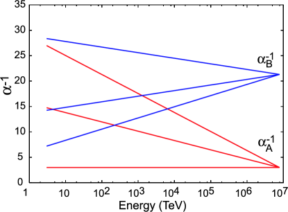
Figure 6: The running of the six gauge couplings, with $\alpha_{A}^{-1}=3$ at the GUT scale.

5.2 The Higgs Mass

Before discussing the Higgs mass bound in this model, we should address the basic structure of the Higgs sector in the presence of the extra doublets. Electroweak symmetry breaking with four Higgs doublets is complicated, and a detailed discussion lies beyond the scope of this work. In [21] the supersymmetric four Higgs doublet model was studied in some detail.

The Yukawa couplings for the Higgs are (ignoring neutrinos)

$$W_{\text{Flavor}}=y_{u}qh_{u}u^{c}+y_{d}qh_{d}d^{c}+y_{e}lh_{e}e^{c}.$$ (51)

We need $h_{u}$, $h_{d}$, and $h_{e}$ to acquire vevs, which constrains the mass terms of the theory. We start with a four Higgs doublet model, with superpotential

$$W_{\mu} = \left(\begin{array}[]{cc}h_{u}&h_{\nu}\end{array}\right)\left(\begin{array}[]{cc}\mu_{ud}&\mu_{ue}\\ \mu_{\nu d}&\mu_{\nu e}\end{array}\right)\left(\begin{array}[]{c}h_{d}\\ h_{e}\end{array}\right).$$ (57)

In the absence of off-diagonal terms, $\mu_{ue}$ and $\mu_{\nu d}$, the quark and lepton Higgs sectors are completely isolated. Thus only $h_{u}$ and $h_{d}$ or $h_{e}$ and $h_{\nu}$ acquire vevs. We therefore need non-zero mixing terms.

To get a limit on the Higgs mass, consider the case where one $\mu$ is much larger than the rest. Then the corresponding pair of Higgs doublets may be integrated out, reducing the Higgs sector to the standard one with two Higgs doublets. This procedure does not lead fine tuning. For the purposes of our discussion, we will give a large mass to $h_{d}h_{\nu}$. This decoupling limit also has the effect of suppressing the masses of the down type quarks relative to the up quarks. Away from this limit many Higgs bosons become light, and the couplings to the gauge bosons are significantly altered. In this case, the LEP limit for the Higgs mass may be altered over sizeable regions of the parameter space – this question certainly warrants further investigation, but will not be pursued here.

For the remainder of this section, we assume the above decoupling limit applies. The limit on the tree-level Higgs mass bound in minimal accelerated unification is significantly relaxed compared to the previous model:

$$\frac{\delta\lambda_{SU(2)}}{\lambda_{SU(2)}}=\frac{g_{2,A}^{2}}{g_{2,{\text{SM}}}^{2}}-1\,\raise 1.29167pt\hbox{$<$\kern-7.5pt\lower 4.30554pt\hbox{$\sim$}}\,1,\hskip 36.135pt\frac{\delta\lambda_{U(1)}}{\lambda_{U(1)}}=\frac{g_{1,A}^{2}}{g_{1,{\text{SM}}}^{2}}-1\,\raise 1.29167pt\hbox{$<$\kern-7.5pt\lower 4.30554pt\hbox{$\sim$}}\,1.$$ (58)

The new bound on the Higgs mass is

$$m_{h^{0}}^{2}\leq 2M_{Z^{0}}^{2}=(128\text{ GeV})^{2},$$ (59)

so we can easily accommodate the LEP II bound without fine-tuning. This considerable improvement over the product unification model is possible because both the $A$ and $B$ gauge couplings split in accelerated unification. This means that $SU(3)_{B}$ remains perturbative for much larger values of the $SU(2)_{A}$ coupling, allowing a larger Higgs mass.

In fact, if we charge the second pair of Higgs doublets under the $B$ groups rather than $A$ groups, the limit is relaxed even further. However, as we will see in Sec. 5.3.2, if both pairs of Higgs doublets are charged under the $A$ groups the model has a natural mechanism to suppress proton decay.

We could also increase the Higgs mass bound by considering $\mathcal{N}\geq 3$ models. This reduces the relative running of the Higgs gauge groups, but lowers the GUT scale at the same time. In addition, as more gauge groups are added, threshold corrections increase and precision unification is lost. In Sec. 5.4 we will see that unification is quite delicate in accelerated unification models, and becomes more so as $\mathcal{N}$ is increased. Thus, there seems to be a tension between increasing the Higgs mass and ensuring accurate gauge coupling unification.

5.3 GUT Scale Physics

At the unification scale the gauge groups unify into $(SU(3)_{C}\times SU(3)_{L}\times SU(3)_{R})_{A,B}$. The usual MSSM matter and Higgs fields combine with additional vector-like matter to form a chiral $\mathbf{27}$ of $[SU(3)]^{3}$. We will assume that this new exotic matter acquires a mass at the GUT scale, so is not relevant to our discussion.

At the unification scale the matter fields, $\Psi$, and Higgs fields, $\Phi$, form the chiral $\mathbf{27}$ of $SU(3)^{3}_{A}$

$$\Psi_{Q}^{\text{SM}},\Phi_{Q}\sim(\mathbf{3}_{C},\overline{\mathbf{3}}_{L})_{A},\hskip 28.90755pt\Psi_{L}^{\text{SM}},\Phi_{L}\sim(\mathbf{3}_{L},\overline{\mathbf{3}}_{R})_{A},\hskip 28.90755pt\Psi_{{Q^{c}}}^{\text{SM}},\Phi_{Q^{c}}\sim(\mathbf{3}_{R},\overline{\mathbf{3}}_{C})_{A}.$$ (60)

The subscript indicates the transformation properties under the gauge charges. Throughout this section capital Greek letters ($\Psi,\Phi,\Sigma$) will denote representations of the trinified GUT group. Lower case Latin letters ($q,h_{u},h_{d}$) will denote fields that transform under $SU(3)\times SU(2)\times U(1)$.

5.3.1 A Trinified NMSSM

The NMSSM is naturally embedded in trinification. The Higgs multiplets contain a singlet $\Phi_{L}$, often dubbed the neutretto. As discussed further in Sec. 5.3.2, the superpotential $\det\Phi_{L}$ gives rise to the NMSSM coupling $nh_{u}h_{d}$. The trilinear $n^{3}$ term does not typically appear. However, a source term for the scalar can appear after SUSY breaking and cause $n$ to acquire a weak scale vev [24].

We start with four Higgs bosons and two singlets at the high scale, and RG flow the superpotential

$$W_{\text{NMSSM}} = \left(\begin{array}[]{cc}h_{u}&h_{\nu}\end{array}\right)\left(\begin{array}[]{cc}(\kappa_{q}n_{q}+\frac{1}{2}\kappa_{q}^{\prime}n_{l})&(\kappa_{l}^{\prime}n_{l}+\kappa_{q}^{\prime}n_{q})\\ (\kappa_{l}^{\prime}n_{l}+\kappa_{q}^{\prime}n_{q})&(\kappa_{l}n_{l}+\frac{1}{2}\kappa_{l}^{\prime}n_{q})\end{array}\right)\left(\begin{array}[]{c}h_{d}\\ h_{e}\end{array}\right)$$ (66)

down to the low scale. We add soft breaking $A$ terms, soft masses for all the fields, and linear soft terms for the singlets.

The analysis of the previous section assumed that the sole new contribution to the quartic coupling came from the gauge sector. However, it is quite possible that an NMSSM-like structure might be a part of the trinified model presented here. In this case, just as in the NMSSM, there is an additional contribution to the quartic coupling. The size of this effect is constrained by the requirement that the coupling not reach a Landau pole below the GUT scale. In this section we will describe how this bound is relaxed in models of accelerated unification – this occurs because the unification scale is lower.

The one loop RGE for the NMSSM–like superpotential coupling $\kappa_{n}$ ($W\ni\kappa_{n}n\bar{h}h$) above the TeV scale is

$$\frac{d}{dt}\kappa_{n}\sim\frac{\kappa_{n}}{16\pi^{2}}\left(4\kappa_{n}^{2}-g_{2,A}^{2}-\frac{3}{5}g_{1,A}^{2}\right).$$ (67)

We have neglected the contribution of SM Yukawa couplings, which depend on which $\kappa$ parameter is being studied. This equation is readily solved in the limit $\kappa_{n}\gg g$,

$$\kappa_{n}^{2}(0)\,\raise 1.29167pt\hbox{$<$\kern-7.5pt\lower 4.30554pt\hbox{$\sim$}}\,\frac{2\pi^{2}}{t_{*}}\Rightarrow\kappa_{n}\,\raise 1.29167pt\hbox{$<$\kern-7.5pt\lower 4.30554pt\hbox{$\sim$}}\,1.15.$$ (68)

This is a modest increase over the standard NMSSM coupling bound. The lowered GUT scale has relaxed the bound on the quartic contribution.

A secondary effect is that the NMSSM coupling is supported by running of the gauge interactions. Accelerated unification increases the gauge couplings, which changes the bounds on $\kappa_{n}$ [4]. However, it is not possible to get the maximal benefit described in [4] in the more restricted accelerated unification framework. From Eq. (67), this would require increasing either the $SU(2)$ or $U(1)$ gauge couplings. However, the size of these couplings is restricted by the condition that $SU(3)_{C\;A,B}$ coupling, which is larger than the $SU(2)$ and $U(1)$ couplings, must be small.

To summarize, the NMSSM couplings can contribute to the Higgs quartic couplings in accelerated unification models.

5.3.2 Proton Decay and the Four Higgs Doublets

In trinified models there is a $\mathbb{Z}_{3}$ symmetry that relates the three gauge couplings to each other. This leads to the introduction of proton decay. This is a model dependent feature – for instance in some string inspired models there is no $\mathbb{Z}_{3}$ symmetry, and the unified gauge coupling is set by the vev of a dilaton. Here, we will take the $\mathbb{Z}_{3}$ symmetry seriously, and consider implications for proton decay. Proton decay occurs through the exchange of colored Higgs triplets (see [25] for a recent study). These triplets will get a GUT-scale mass which, depending on the flavor structure of the model, may not be enough to suppress proton decay via dimension five and six operators, in which case further model building is necessary. As we will see, the addition of a second pair of Higgs doublets can easily suppress proton decay in our accelerated unification model.

To see how this occurs, we must first discuss the implementation of flavor in this model. There are two pairs of Higgs doublets in accelerated unification. We will couple one pair, $\Phi_{L}^{l}$, to the leptons and the other pair, $\Phi_{L}^{q}$, to the quarks. Assuming that the flavor structure obeys the $\mathbb{Z}_{3}$ symmetry, the MSSM Yukawa interactions are schematically given by the following superpotential terms

$$W_{\text{flavor}} = y_{Q}\,(\Psi_{Q}^{\text{SM}}\Phi^{q}_{L}\Psi_{Q^{c}}^{\text{SM}}+\Psi_{L}^{\text{SM}}\Phi^{q}_{Q^{c}}\Psi_{Q}^{\text{SM}}+\Psi_{Q^{c}}^{\text{SM}}\Phi^{q}_{Q}\Psi_{L}^{\text{SM}})$$ (69)

$$+y_{L}\,(\Psi_{L}^{\text{SM}}\Psi_{L}^{\text{SM}}\Phi^{l}_{L}+\Psi_{Q}^{\text{SM}}\Psi_{Q}^{\text{SM}}\Phi^{l}_{Q}+\Psi_{Q^{c}}^{\text{SM}}\Psi_{Q^{c}}^{\text{SM}}\Phi^{l}_{Q^{c}}).$$

At the level of the superpotential, baryon number symmetry is exact if we assign $\Phi_{Q}^{q}$ and $\Phi_{Q^{c}}^{q}$ baryon number $\pm\frac{1}{3}$ and assign $\Phi_{Q}^{l}$ and $\Phi_{Q^{c}}^{l}$ baryon number $\mp\frac{2}{3}$. We have suppressed proton decay through a missing partner mechanism, as long as the colored triplet Higgs boson does not mix quark and lepton sectors at the GUT scale.

However, the $q$ and $l$ Higgs sectors must not be completely decoupled: if this were the case, then only one Higgs pair would acquire a vev at the electroweak scale, leaving the second sector massless. Moreover, we need $\mu$ terms for Higgs fields, which may be generated by giving a vev to the NMSSM fields in both Higgs sectors. The trilinear superpotential is

$$W_{\text{NMSSM}} = \frac{1}{3}\kappa_{l}(\Phi_{L}^{l})^{3}+\frac{1}{3}\kappa_{q}(\Phi_{L}^{q})^{3}+\frac{1}{2}\kappa^{\prime}_{l}(\Phi_{L}^{l})^{2}\Phi_{L}^{q}+\frac{1}{2}\kappa^{\prime}_{q}(\Phi_{L}^{q})^{2}\Phi_{L}^{l}+\text{ cyclic.}$$ (70)

$$\supset \left(\begin{array}[]{cc}h_{u}&h_{\nu}\end{array}\right)\left(\begin{array}[]{cc}(\kappa_{q}n_{q}+\frac{1}{2}\kappa_{q}^{\prime}n_{l})&(\kappa_{l}^{\prime}n_{l}+\kappa_{q}^{\prime}n_{q})\\ (\kappa_{l}^{\prime}n_{l}+\kappa_{q}^{\prime}n_{q})&(\kappa_{l}n_{l}+\frac{1}{2}\kappa_{l}^{\prime}n_{q})\end{array}\right)\left(\begin{array}[]{c}h_{d}\\ h_{e}\end{array}\right).$$ (76)

The low energy theory is similar to the NMSSM, but without $n^{3}$ terms. The cyclic permutations of the interactions in Eq. (70) no longer preserve baryon number exactly. The $\kappa_{l}$ and $\kappa_{q}$ interactions give rise to dimension seven $p\rightarrow e^{+}\bar{\nu}\bar{\nu}$ and $n\rightarrow\bar{n}$ oscillations. The $\kappa_{q}^{\prime}$ and $\kappa_{l}^{\prime}$ interactions lead to dimension seven proton decay processes of the form $p\rightarrow K^{+}\nu$. All of these come with three powers of Yukawa couplings, and three powers of the GUT scale in the denominator.

For example, consider the baryon number violating operator

$$W_{\not{B}}=\frac{qqqqd^{c}e^{c}}{M^{3}}+\cdots,$$ (77)

which is generated by the diagram in Fig. 7. The interactions in this diagram come from the cyclic permutations of the terms in $W_{Y}$ and $W_{\text{NMSSM}}$. Taking into account the small Yukawa couplings and CKM mixings, this leads to a proton lifetime

$$\tau_{p}\sim 10^{70}\text{yrs.}\left(\frac{M_{H_{C}}}{M_{\text{GUT}}}\right)^{6},$$ (78)

where $M_{H_{C}}$ is the mass of the colored Higgs triplet mediating the proton decay. We can therefore take the mass of the Higgs triplet to be quite low without leading to unacceptable proton decay, unlike in the MSSM.

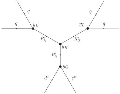
Figure 7: A leading operator contributing to baryon number violation.

5.4 Precision Unification

In Sec. 4.3, we showed that the effects of higher loop running are encoded in the anomalous dimensions of the light fields. In accelerated unification models, we must also include contributions from the new light fields. In addition to the second pair of Higgs doublets, there are also pseudo-Goldstone bosons (PGBs), as we will now discuss. The mass of these particles is the largest source of imprecision in the gauge coupling unification prediction.

The superpotential of Eq. (14) has a global $SU(3)$ symmetry. The breaking to the diagonal will in general give rise to Goldstone bosons. In the $SU(3)$ color sector, all such particles get a mass from gauge interactions. For the $SU(3)_{L}$ and $SU(3)_{R}$ sectors, this is not the case. The condition to lift these PGBs is $\det\mu_{I}\neq 0$. While renormalization group evolution splits the $\mu$ parameters, it will not cause the determinant to flow to a non-zero value, although GUT-scale threshold corrections could make this determinant non-zero. The mass of the PGBs will then RG evolve as $\det\mu$ evolves. If the $SU(3)$ breaking couplings are larger than the $SU(3)$ preserving superpotential couplings, then $\det\mu$ will flow away from zero. We will not specify the mass of these particles, but will summarize their possible effect on unification at the end of this section.

We now apply the formalism of Appendix A to accelerated unification. The difference between the $SU(3)$ and $SU(2)$ couplings is

$$\Delta^{32}\equiv\frac{8\pi^{2}}{g_{3}^{2}(\mu)}-\frac{8\pi^{2}}{g_{2}^{2}(\mu)} = \left[\Delta b^{32}_{\text{MSSM}}\log\frac{\Lambda}{\mu}+\Delta b^{32}_{\text{AU}}\log\frac{\Lambda}{\langle\Sigma\rangle}\right]$$ (79)

$$+\delta z_{\psi}^{32}+\delta z_{h}^{32}+3\log\frac{g^{2}_{A}(\Lambda)g^{2}_{B}(\Lambda)}{g^{2}_{3}(\mu)}-2\log\frac{g^{2}_{A}(\Lambda)g^{2}_{B}(\Lambda)}{g^{2}_{2}(\mu)}$$

$$+\delta b^{32}_{h}\log\frac{\langle\Sigma\rangle}{\mu_{H}}+\delta b^{32}_{{\text{PGB}}_{L}}\log\frac{\langle\Sigma\rangle}{m_{{\text{PGB}}_{L}}},$$

where $\mu_{H}$ is the mass of the second pair of Higgs doublets, $\Delta b^{32}_{\text{MSSM}}$ is the difference between beta functions in the MSSM, and $\Delta b^{32}_{\text{AU}}\equiv\Delta b^{32}_{A}+\Delta b^{32}_{B}-\Delta b^{32}_{\text{MSSM}}$ is the difference between beta function coefficients for the additional accelerated unification fields. When $\mathcal{N}=2$, $\Delta b^{32}_{\text{AU}}=\Delta b^{32}_{\text{MSSM}}=-4$. The quantity in brackets reproduces the MSSM one loop prediction. The $\log Z$’s of the light fields

$$\delta z_{\psi}^{32}=\frac{1}{2}\log\prod_{f=1}^{3}\frac{Z_{u^{c}_{f}}Z_{d^{c}_{f}}}{Z_{q_{f}}Z_{l_{f}}},\hskip 28.90755pt\delta z_{h}^{32}=-\frac{1}{2}\log Z_{h_{u}}Z_{h_{d}}Z_{h_{e}}Z_{h_{\nu}},$$ (80)

are evaluated by integrating the anomalous dimensions from $\Lambda$ down to $\mu$. The final terms arise from the second pair of Higgs doublets and the PGBs in the left sector, with

$$\delta b^{32}_{h}=-1\hskip 36.135pt\delta b^{32}_{{\text{PGB}}_{L}}=-1.$$ (81)

If the masses of these particles were precisely at the scale of diagonal breaking, they would not contribute any additional deviation. However, in the model presented here the masses are essentially free parameters. The mass of the extra Higgs multiplet depends sensitively on the values of the various $\mu$ parameters. A similar calculation for the $SU(2)$ and $U(1)$ couplings yields,

$$\Delta^{21}\equiv\frac{8\pi^{2}}{g_{2}^{2}(\mu)}-\frac{8\pi^{2}}{g_{1}^{2}(\mu)} = \left[\Delta b^{21}_{\text{MSSM}}\log\frac{\Lambda}{\mu}+\Delta b^{21}_{\text{AU}}\log\frac{\Lambda}{\langle\Sigma\rangle}\right]$$ (82)

$$+ 2\log\frac{g^{2}_{A}(\Lambda)g^{2}_{B}(\Lambda)}{g^{2}_{2}(\mu)}+\delta z_{\psi}^{21}+\delta z_{h}^{21}+\delta b^{21}_{h}\log\frac{\langle\Sigma\rangle}{\mu_{H}}$$

$$+ \delta b^{21}_{{\text{PGB}}_{L}}\log\frac{\langle\Sigma\rangle}{m_{{\text{PGB}}_{L}}}+\delta b^{21}_{{\text{PGB}}_{R}}\log\frac{\langle\Sigma\rangle}{m_{{\text{PGB}}_{R}}},$$ (83)

with $\Delta b^{21}_{\text{MSSM}}=\Delta b^{21}_{\text{AU}}=-18/5$. The $\log Z$s of the light fields are

$$\delta z_{\psi}^{21}=\frac{1}{5}\log\Pi_{f}\frac{Z_{q_{f}}^{7}Z_{l_{f}}}{Z_{u^{c}_{f}}^{4}Z_{d^{c}_{f}}Z_{e^{c}}^{3}},\hskip 28.90755pt\delta z_{h}^{21}=\frac{1}{5}\log Z_{h_{u}}Z_{h_{d}}Z_{h_{e}}Z_{h_{\nu}}.$$ (84)

Finally, the additional Higgs doublets and the PGBs contribute to the beta function coefficients

$$\delta b^{21}_{h}=\frac{2}{5},\hskip 36.135pt\delta b^{21}_{{\text{PGB}}_{L}}=\frac{2}{5},\hskip 36.135pt\delta b^{21}_{{\text{PGB}}_{R}}=-\frac{12}{5}.$$ (85)

For the moment, let us assume that these additional light fields are degenerate with the remainder of the multiplet. In this case, we find the ratio

$$\frac{\Delta^{32}}{\Delta^{21}}\simeq 0.721.$$ (86)

This result is insensitive to the choice of ${\alpha_{A}^{-1}}$. Making the more reasonable choice that the PGBs and the extra Higgs multiplet are two $e$-folds below the rest of the multiplet, we find $\Delta^{32}/\Delta^{21}=0.716$. Again, we conclude that none of the calculable corrections to unifications are very large. However, if the masses deviate too far from the diagonal breaking scale the corrections from the PGBs can be non-negligible. Moreover, when $\mathcal{N}>2$, there are more PGBs, which can amplify these effects.

There are of course additional threshold corrections. As before, there are the corrections from SUSY breaking. Also, since there are two copies of $SU(3)^{3}$ near the GUT scale, the high energy particle content is double that of the MSSM. So, the naive expectation for GUT scale threshold corrections is that they should be roughly double those of the MSSM. An interesting possibility arises in accelerated unification that is not present in the MSSM. In Sec. 5.3.2 we showed that proton decay is suppressed, so it is possible for the colored Higgs triplets that mediate proton decay to be much lighter than the GUT scale. This leads to a threshold correction that improves the unification of the couplings. In the minimal SU(5) GUT, such a threshold correction would be desirable, but is forbidden by proton decay [26].

6 Conclusions

Gauge coupling unification places a natural constraint on the structure of potential gauge extensions of the MSSM. Moreover, it limits the size of the new gauge couplings under which the Higgs boson may be charged. The result is that the Higgs mass cannot be too heavy, even in models with extended gauge structure. Accelerated unification seems to be the best hope for realizing a heavier Higgs mass, but due to the presence of pseudo-Goldstone bosons, unification becomes somewhat delicate.

In the models discussed here, a host of new states associated with the breaking should be found at the 3-10 TeV scale. In the accelerated unification model, it is likely that the lightest state would be one of the PGBs. The precise mass of this particle depends on the breaking of the GUT symmetry. We now discuss precision electroweak constraints, which set the mass of the new vector bosons.

6.1 Constraints

Precision electroweak constraints on these models arise from interactions between the heavy vector bosons and the Standard Model fermions and Higgs. One might worry that these considerations significantly constrain the theory; in order to maximize non-decoupling $D$-terms we need the Standard Model gauge couplings to be as strong as possible, which means that the heavy vector bosons couple with $\mathcal{O}(1)$ strength to the Standard Model fermions. However, because these new vectors are not responsible for cutting off the gauge quadratic divergences to the Higgs, they can be quite heavy without fine-tuning. Instead, the heavy vectors cut off divergent contributions to the Higgs mass arising from the modified quartic coupling, so the vectors may comfortably lie in the 3 – 10 TeV range.

To see this, it is useful to introduce mixing angles $\theta_{i}$ for the gauge fields, obeying

$$\sin^{2}\theta_{i}=\frac{g^{2}_{i,{\text{SM}}}}{g^{2}_{i,A}},\hskip 21.68121pt\cos^{2}\theta_{i}=\frac{g^{2}_{i,{\text{SM}}}}{g^{2}_{i,B}}.$$ (87)

The heavy vectors, which we denote $A_{i}$, couple to the to the MSSM via the interaction

$$\mathcal{L}_{{\text{eff}}}=-g_{i,{\text{SM}}}\cot\theta_{i}\,A_{i}^{\mu}j_{\mu i,{\text{SM}}}+\frac{g_{i,SM}^{2}f^{2}}{\sin 2\theta_{i}}(A_{i}^{\mu})^{2}.$$ (88)

At low energies the $A_{i}$ may be integrated out to give the current-current interaction

$$\mathcal{L}_{\text{eff}}=\frac{\cos^{4}\theta_{i}}{2f^{2}}j^{\mu}_{i,{\text{SM}}}j_{\mu\text{SM}}.$$ (89)

These terms contribute to the $W,Y,Z$ extended oblique corrections, which are constrained experimentally, implying a constraint [27]

$$\frac{f_{L,R}}{\cos^{2}\theta_{L,R}}\,\raise 1.29167pt\hbox{$>$\kern-7.5pt\lower 4.30554pt\hbox{$\sim$}}\,3.5\text{ TeV }.$$ (90)

Thus even for $\cos\theta_{L,R}\sim 1$ the breaking scales can be 3.5 TeV and vectors will be under 10 TeV.

6.2 Future Directions

There are several potential directions for future work. As noted in the text, the theories under consideration are very similar to deconstructed models of gaugino mediation. It would be interesting to determine whether the link fields can communicate SUSY breaking to the MSSM. Once a SUSY breaking scenario is specified, either this mechanism or another, it would be possible to discuss spectroscopy and unification in further detail. It would also be of interest to explore the supersymmetric four Higgs doublet in more detail. In principle, the experimental limits on the Higgs boson can be modified.

Appendix A Precision Unification and Holomorphy

In supersymmetric theories, threshold corrections are constrained by holomorphy. This technique can be applied to calculate corrections to unification in any model where holomorphy is a useful constraint (i.e. when there are large supersymmetric masses).

Our first result is that threshold effects from mass splittings cancel against higher loop corrections [22, 23]. To see this, consider the exact NSVZ beta function [22]

$$\beta_{g}=\frac{g^{3}}{16\pi^{2}}\frac{b_{0}-\sum_{a}T_{2}(a)\gamma_{a}}{1-C_{2}\frac{g^{2}}{8\pi^{2}}},$$ (91)

where $b_{0}=-3C_{2}+\sum_{a}T_{2}(a)$. This can be integrated to give

$$\frac{8\pi^{2}}{g^{2}(\mu)}+C_{2}\log g^{2}(\mu)=\frac{8\pi^{2}}{g^{2}(\Lambda)}+C_{2}\log g^{2}(\Lambda)+b_{0}\log\frac{\Lambda}{\mu}-\sum_{a}T_{2}(a)\log Z_{a}(\mu,\Lambda).$$ (92)

Now consider integrating out a massive matter field (like the link fields, $\Sigma$). Gauge couplings are matched at the physical mass of the field, $m_{r}$, which differs from the holomorphic mass $m$ (which appears in the superpotential) by a factor of the wave function renormalization: $m=Z(m_{r},\Lambda)m_{r}$. Thus, the $\log Z$ that appears in the NSVZ formula can be combined with a holomorphic mass to recover a running mass. So, it is possible to write a RG invariant matching equation exclusively in terms of holomorphic quantities:

$$\frac{8\pi^{2}}{g^{2}_{\text{LE}}(\Lambda)}+C_{2}\log g^{2}_{\text{LE}}(\Lambda)=\frac{8\pi^{2}}{g^{2}_{\text{HE}}(\Lambda)}+C_{2}\log g^{2}_{\text{HE}}(\Lambda)-\log\frac{\Lambda}{m}.$$ (93)

Here $g^{2}_{\text{LE}}(\Lambda)$ and $g^{2}_{\text{HE}}(\Lambda)$ are the low energy and high energy gauge couplings defined at the cut-off $\Lambda$; they have one loop beta functions $b_{0,{\text{LE}}}$ and $b_{0,{\text{HE}}}$ respectively that differ by one. Using the NSVZ beta function, one can verify that Eq. (93) is equivalent the matching the high energy and low energy gauge couplings at the physical mass scale. However, Eq. (93) is valid all scales, including at the cut-off, where there clearly has been no running to split $m$. Thus, complete GUT multiplets will lead to a small deviation from the MSSM prediction. The dominant effect is indirect: the gauge coupling RG trajectories are deflected by the presence of the $\Sigma$ fields, which in turn contributes to the last term in Eq. (92) for the light MSSM fields.

A second potential source of modifications to unification comes from the breaking of extended gauge symmetry. We must apply a matching condition when $G\times G_{GUT}\rightarrow G_{SM}$. The usual matching conditions

$$\frac{8\pi^{2}}{g^{2}(m_{V,{\text{phys}}})}=\frac{8\pi^{2}}{g_{A}^{2}(m_{V,{\text{phys}}})}+\frac{8\pi^{2}}{g_{B}^{2}(m_{V,{\text{phys}}})},\hskip 28.90755pt\left(\frac{8\pi^{2}}{g^{2}(m_{X,{\text{phys}}})}\right)_{-}=\left(\frac{8\pi^{2}}{g^{2}(m_{X,{\text{phys}}})}\right)_{+},$$ (94)

are reproduced by the RG invariant matching equation

$$\frac{8\pi^{2}}{g^{2}(\Lambda)}+C_{2}\log g^{2}(\Lambda)=\frac{8\pi^{2}}{g_{A}^{2}(\Lambda)}+C_{2}\log g_{A}^{2}(\Lambda)+\frac{8\pi^{2}}{g_{B}^{2}(\Lambda)}+C_{2}^{B}\log g_{B}^{2}(\Lambda)-C_{2}^{B}\log\frac{\Lambda^{2}}{\langle\Sigma\Sigma^{c}\rangle}.$$ (95)

Here $\langle\Sigma\rangle$ and $\langle\Sigma^{c}\rangle$ are the vevs of the fields that break the gauge symmetry, and we have used $C_{2}^{SM}=C_{2}^{A}\equiv C_{2}$. We have also used expressions for the renormalized gauge boson masses:

$$M_{V}^{2} = Z(M_{V},\Lambda)\langle\Sigma\Sigma^{c}\rangle(g_{A}^{2}+g_{B}^{2})_{M_{V}^{2}}$$ (96)

$$M_{X}^{2} = Z(M_{X},\Lambda)\langle\Sigma\Sigma^{c}\rangle(g_{B}^{2})_{M_{V}^{2}}.$$ (97)

Applying the above RG invariant matching condition gives rise to Eq. (42) for product unification.

For accelerated unification, the RG invariant matching equation is similar. The analog of Eq. (95) is:

$$\frac{8\pi^{2}}{g^{2}(\mu)}+C_{2}\log g^{2}(\mu) = \frac{8\pi^{2}}{g_{A}^{2}(\Lambda)}+C_{2}\log g_{A}^{2}(\Lambda)+\frac{8\pi^{2}}{g_{B}^{2}(\Lambda)}+C_{2}\log g_{B}^{2}(\Lambda)$$ (98)

$$-C_{2}\log\frac{\Lambda^{2}}{\langle\Sigma\Sigma^{c}\rangle}+b_{\phi}\log\frac{\Lambda}{m_{\phi}}$$

$$+b_{0,\text{light}}\log\frac{\Lambda}{\mu}-\sum_{a}T_{2}(a)\log Z_{a}(\mu,\Lambda).$$

We have used $C_{2}=C^{A}_{2}=C^{B}_{2}$, and integrated out the $\phi$ multiplet at its holomorphic mass. In this case, there are additional light states in the sum, namely the pseudo-Goldstone bosons and Higgs multiplets discussed in the text.

Appendix B D-Terms and Tadpoles

In this appendix, we give general expressions for the masses of $M_{V_{H}}$, $S$, $\phi$, and $\eta$, taking into account the possibility of a SUSY breaking induced tadpole for the $S$ field. After including the supersymmetry breaking, as in Eq. (29), and restricting attention to the field $S$, there is a linear source term:

$$W = ((a-b)\mu-m^{2})\theta^{2}\sqrt{6}\frac{\mu}{\lambda}S-\mu(1+(2a-b)\theta^{2})\frac{S^{2}}{2}+\frac{\lambda}{3\sqrt{6}}(1+a\theta^{2})S^{3}$$

$$K = (1+m^{2}\theta^{4})S^{\dagger}S.$$ (99)

We may shift $S$ by a constant to remove this term,

$$S\rightarrow S+J\hskip 36.135ptJ=\frac{\sqrt{6}}{\lambda}(-j_{S}\mu+j_{F}\mu^{2}\theta^{2}).$$ (100)

Solving for $j_{S}$ and $j_{F}$,

$$j_{F}=-j_{S}-j_{S}^{2}$$ (101)

$$\frac{\mu^{2}-m^{2}+(2a-b)\mu}{\mu^{2}}j_{S}+\Big{(}3+\frac{a}{\mu}\Big{)}j_{S}^{2}+2j_{S}^{3}=\frac{(m^{2}+(b-a)\mu)}{\mu^{2}}.$$ (102)

This shift affects the Kahler term for $V_{H}$:

$$K=g_{H}^{2}\frac{\mu^{2}}{\lambda^{2}}\left(1+j_{S}\right)^{2}\left(1+\left(m^{2}+\mu^{2}\frac{j_{F}^{2}}{(1+j_{S})^{2}}\right)\theta^{4}\right)\text{ Tr }V_{H}^{2}.$$ (103)

This expression summarizes how SUSY breaking is communicated to the vector multiplet. We must also check that the other scalar masses

$$\frac{m_{S}^{2}}{\mu^{2}} = \Big{(}1+2j_{S}\Big{)}^{2}+\frac{m^{2}}{\mu^{2}}\pm\Big{(}\frac{2a-b}{\mu}-2\Big{(}j_{F}-\frac{a}{\mu}j_{S}\Big{)}\Big{)}$$

$$\frac{m_{\phi}^{2}}{\mu^{2}} = \Big{(}2+j_{S}\Big{)}^{2}+\frac{m^{2}}{\mu^{2}}\pm\Big{(}\frac{a+b}{\mu}-\Big{(}j_{F}-\frac{a}{\mu}j_{S}\Big{)}\Big{)}$$

$$\frac{m_{\eta}^{2}}{\mu^{2}} = \left((3+2j_{S})^{2}+2j_{S}^{2}+\frac{m^{2}}{\mu^{2}}\right)\mp 3\left[4j_{S}^{2}-5j_{S}-\frac{m^{2}}{\mu^{2}}+(1+j_{S})\frac{a}{\mu}\right]$$ (104)

remain positive. It may be shown that these masses remain positive over large regions of parameter space. However, as described in the text, it is sufficient to note that when $a=0$ and $j_{S}=j_{F}=0$ the masses are positive whenever $m^{2}>-\mu^{2}/2$.

References

- [1] R. Barate et al. [ALEPH Collaboration], Phys. Lett. B 565, 61 (2003) [arXiv:hep-ex/0306033].
- [2] G. L. Kane, B. D. Nelson, L. T. Wang and T. T. Wang, arXiv:hep-ph/0407001.
- [3] P. Batra, A. Delgado, D. E. Kaplan and T. M. P. Tait, JHEP 0402, 043 (2004) [arXiv:hep-ph/0309149].
- [4] P. Batra, A. Delgado, D. E. Kaplan and T. M. P. Tait, JHEP 0406, 032 (2004) [arXiv:hep-ph/0404251].
- [5] R. Harnik, G. D. Kribs, D. T. Larson and H. Murayama, arXiv:hep-ph/0311349; S. Chang, C. Kilic and R. Mahbubani, arXiv:hep-ph/0405267.
- [6] A. Birkedal, Z. Chacko and M. K. Gaillard, arXiv:hep-ph/0404197.
- [7] N. Polonsky and S. Su, Phys. Lett. B 508, 103 (2001) [arXiv:hep-ph/0010113]; P. Langacker, N. Polonsky and J. Wang, Phys. Rev. D 60, 115005 (1999) [arXiv:hep-ph/9905252].
- [8] S. Dimopoulos and H. Georgi, Nucl. Phys. B 193, 150 (1981); S. Dimopoulos, S. Raby and F. Wilczek, Phys. Rev. D 24, 1681 (1981).
- [9] L. Randall. Talk at SUSY 2002.
- [10] N. Arkani-Hamed, A. G. Cohen and H. Georgi, arXiv:hep-th/0108089.
- [11] B. Grinstein, Nucl. Phys. B 206, 387 (1982). A. Masiero, D. V. Nanopoulos, K. Tamvakis and T. Yanagida, Phys. Lett. B 115, 380 (1982).
- [12] P. Fayet, Nucl. Phys. B 113, 135 (1976); H. P. Nilles, M. Srednicki and D. Wyler, Phys. Lett. B 120, 346 (1983). J. P. Derendinger and C. A. Savoy, Nucl. Phys. B 237, 307 (1984). J. R. Ellis, J. F. Gunion, H. E. Haber, L. Roszkowski and F. Zwirner, Phys. Rev. D 39, 844 (1989).
- [13] J. R. Ellis, G. Ridolfi and F. Zwirner, Phys. Lett. B 257, 83 (1991); Y. Okada, M. Yamaguchi and T. Yanagida, Prog. Theor. Phys. 85, 1 (1991); H. E. Haber and R. Hempfling, Phys. Rev. Lett. 66, 1815 (1991).
- [14] J. R. Espinosa and M. Quiros, Phys. Rev. Lett. 81, 516 (1998) [arXiv:hep-ph/9804235].
- [15] G. L. Kane, C. F. Kolda and J. D. Wells, Phys. Rev. Lett. 70, 2686 (1993) [arXiv:hep-ph/9210242].
- [16] S. Eidelman et al. [Particle Data Group Collaboration], Phys. Lett. B 592, 1 (2004).
- [17] N. Arkani-Hamed, A. G. Cohen and H. Georgi, Phys. Rev. Lett. 86, 4757 (2001) [arXiv:hep-th/0104005].
- [18] C. Csaki, J. Erlich, C. Grojean and G. D. Kribs, Phys. Rev. D 65, 015003 (2002) [arXiv:hep-ph/0106044]; H. C. Cheng, D. E. Kaplan, M. Schmaltz and W. Skiba, Phys. Lett. B 515, 395 (2001) [arXiv:hep-ph/0106098].
- [19] D. E. Kaplan, G. D. Kribs and M. Schmaltz, Phys. Rev. D 62, 035010 (2000) [arXiv:hep-ph/9911293].
- [20] S. L. Glashow, Print-84-0577 (BOSTON); G. Lazarides, C. Panagiotakopoulos and Q. Shafi, Phys. Lett. B 315, 325 (1993) [Erratum-ibid. B 317, 661 (1993)] [arXiv:hep-ph/9306332].
- [21] M. Drees, Int. J. Mod. Phys. A 4, 3635 (1989).
- [22] M. A. Shifman and A. I. Vainshtein, Nucl. Phys. B 277, 456 (1986) [Sov. Phys. JETP 64, 428 (1986 ZETFA,91,723-744.1986)]. V. A. Novikov, M. A. Shifman, A. I. Vainshtein and V. I. Zakharov, Nucl. Phys. B 229, 381 (1983). V. A. Novikov, M. A. Shifman, A. I. Vainshtein and V. I. Zakharov, Nucl. Phys. B 260, 157 (1985) [Yad. Fiz. 42, 1499 (1985)]. M. A. Shifman, A. I. Vainshtein and V. I. Zakharov, Phys. Lett. B 166, 334 (1986).
- [23] N. Arkani-Hamed and H. Murayama, Phys. Rev. D 57, 6638 (1998) [arXiv:hep-th/9705189]. N. Arkani-Hamed and H. Murayama, JHEP 0006, 030 (2000) [arXiv:hep-th/9707133].
- [24] J. Bagger and E. Poppitz, Phys. Rev. Lett. 71, 2380 (1993) [arXiv:hep-ph/9307317]. J. Bagger, E. Poppitz and L. Randall, Nucl. Phys. B 455, 59 (1995) [arXiv:hep-ph/9505244]. V. Jain, Phys. Lett. B 351, 481 (1995) [arXiv:hep-ph/9407382]. C. Panagiotakopoulos and K. Tamvakis, Phys. Lett. B 469 (1999) 145 [arXiv:hep-ph/9908351]. C. Panagiotakopoulos and A. Pilaftsis, Phys. Rev. D 63, 055003 (2001) [arXiv:hep-ph/0008268]. A. Dedes, C. Hugonie, S. Moretti and K. Tamvakis, Phys. Rev. D 63, 055009 (2001) [arXiv:hep-ph/0009125].
- [25] T. Roy, arXiv:hep-ph/0408291.
- [26] H. Murayama and A. Pierce, Phys. Rev. D 65, 055009 (2002) [arXiv:hep-ph/0108104].
- [27] R. Barbieri, A. Pomarol, R. Rattazzi and A. Strumia, arXiv:hep-ph/0405040.