hep-ph/0409126

Curing the Ills of Higgsless Models:
the $S$ Parameter and Unitarity

Giacomo Cacciapaglia^a, Csaba Csáki^a, Christophe Grojean^b,c,
and John Terning^d

^a Institute for High Energy Phenomenology
Newman Laboratory of Elementary Particle Physics
Cornell University, Ithaca, NY 14853, USA

^b Service de Physique Théorique, CEA Saclay, F91191 Gif–sur–Yvette, France

^c Michigan Center for Theoretical Physics, Ann Arbor, MI 48109, USA
^d Theory Division T-8, Los Alamos National Laboratory, Los Alamos, NM 87545, USA

cacciapa@mail.lns.cornell.edu, csaki@lepp.cornell.edu, grojean@spht.saclay.cea.fr, terning@lanl.gov

We consider various constraints on Higgsless models of electroweak symmetry breaking based on a bulk SU(2)${}_{L}\times$SU(2)${}_{R}\times$U(1)_B-L gauge group in warped space. First we show that the $S$ parameter which is positive if fermions are localized on the Planck brane can be lowered (or made vanishing) by changing the localization of the light fermions. If the wave function of the light fermions is almost flat their coupling to the gauge boson KK modes will be close to vanishing, and therefore contributions to the $S$ parameter will be suppressed. At the same time the experimental bounds on such $Z^{\prime}$ and $W^{\prime}$ gauge bosons become very weak, and their masses can be lowered to make sure that perturbative unitarity is not violated in this theory before reaching energies of several TeV. The biggest difficulty of these models is to incorporate a heavy top quark mass without violating any of the experimental bounds on bottom quark gauge couplings. In the simplest models of fermion masses a sufficiently heavy top quark also implies an unacceptably large correction to the $Zb\bar{b}$ vertex and a large splitting between the KK modes of the top and bottom quarks, yielding large loop corrections to the $T$-parameter. We present possible directions for model building where perhaps these constraints could be obeyed as well.

1 Introduction

The quest to uncover the origin of electroweak symmetry breaking has been at the forefront of particle physics for 25 years, and after a tremendous amount of theoretical effort it is clearer than ever that we will need experiments to answer the question. This has been further emphasized by the explosion in the last few years of a plethora of alternative electroweak symmetry breaking scenarios, which bear little resemblance to the three traditional solutions: the standard model (SM), the minimal supersymmetric standard model, and the technicolor scenario. In addition to large extra dimensions [1], warped extra dimensions [2], gauge component Higgses [3], “little” Higgses [4], and “fat” Higgses [5], one of the most recent proposals, and in some ways most radical, is the Higgsless scenario [6, 7, 8, 9]. These models take advantage of the fact that with a Higgs localized in an extra dimension, there exists a limit where the Higgs decouples from $WW$ scattering but with a finite $W$ mass. The limit is achieved by taking the Higgs vacuum expectation value (VEV) to $\infty$. In this limit the gauge symmetry breaking amounts to imposing Dirichlet boundary conditions on the gauge field at one end of the extra dimension [6]. Quarks and leptons can receive masses from boundary conditions as well [8, 9, 10]. Since there is no contribution to $WW$ scattering from a Higgs boson, these scattering amplitudes are unitarized by another mechanism: exchanges of the Kaluza-Klein (KK) tower of gauge bosons [6, 11]. Taking the extra dimension to be anti-de Sitter (AdS) with an SU(2)${}_{L}\times$SU(2)${}_{R}\times$U(1)_B-L gauge group in the bulk has the dual advantage of raising the KK masses to phenomenologically acceptable levels (and thus solving the “little hierarchy problem”) and also imposing a custodial isospin symmetry which protects the ratio of the $W$ and $Z$ masses. The presence of this custodial isospin symmetry follows from the AdS/CFT correspondence [12]. Further properties of Higgsless models and different variations have been explored in refs. [13, 14, 15, 16, 17, 18, 19, 20, 21, 22, 23, 24, 25, 26].

This scenario shares many common features with technicolor models: in fact it can be thought of as a gravity dual of technicolor models, except that there are regions of parameter space where the theory is in fact weakly coupled and calculable. The leading corrections to electroweak precision observables have been calculated for the simplest setup in refs. [13, 14, 15], where a large positive contribution to the $S$ parameter has been found. This can be lowered by introducing a brane induced kinetic term on the TeV brane for the $B-L$ gauge group [15], however at the price of lowering the mass of one of the $Z^{\prime}$ modes to levels already excluded by LEP2 [27] and/or Tevatron[28].

In this paper we point out that one can in fact easily eliminate the large contributions to the $S$ parameter by changing the position of the light fermions. The reason behind this is simple: the oblique correction parameters $S,T,U$ on their own are meaningless until the normalization of the couplings between the fermions and the gauge bosons is fixed. An overall shift in the fermion gauge boson couplings can be reabsorbed in the oblique correction parameters and thus effectively change the predicted values of $S,T,U$. This is exactly what happens when one changes the localization parameters of the light fermions. Until now all calculations of the oblique parameters in Higgsless models [13, 14, 15, 16, 17] or variations [18, 19, 20, 21] have assumed that the fermions are strictly localized on the Planck brane, in which case one obtains a positive $S$ parameter. However, it has been known for quite a while [29] that if fermions are localized on the TeV brane then the $S$ parameter in the Randall-Sundrum model is in fact negative. Therefore it should be expected that there should be an intermediate position where $S$ exactly vanishes. This actually happens when the fermion wave functions are “flat”, corresponding to localization parameter $c=1/2$. This is just a simple consequence of the orthogonality of the KK mode wave functions of the gauge bosons: when $c=1/2$ the coupling of the KK gauge bosons to the fermions vanishes, eliminating any possible additional LEP or Tevatron constraints on this setup. The fact that for $c=1/2$ the $S$ parameter generically vanishes was first mentioned in [12].

Another issue frequently discussed regarding Higgsless models is the question whether the first KK mode of the gauge bosons is light enough to actually unitarize the WW scattering amplitudes at weak coupling [13, 16, 26]. It follows from general arguments that the asymptotically growing terms in the individual scattering amplitudes always cancel, however one also needs to make sure that the finite terms are sufficiently small and in the perturbative regime, even after taking a coupled channel analysis into account. In this paper we point out that by adjusting the value of the bulk curvature scale one can lower the masses of the KK gauge bosons to a few hundred GeV, without conflicting the direct search bounds due to the weak coupling of the light fermions to the KK modes, while the $S$ parameter can be made vanishing by adjusting the localization parameter $c$ of the fermions. This way we show that the two most commonly quoted problematic aspects of Higgsless models are in fact easily avoidable.

Rather, we find that the most serious issue of these models is the inclusion of a heavy top quark. In the simplest implementation of fermion masses one will generically either find a top quark mass that is too low, or a correction to the $Zb\bar{b}$ vertex that deviates from the SM prediction beyond allowable levels. Furthermore, in most cases when the top quark is sufficiently split from the bottom quark there is also a large splitting in the KK modes of the top and bottom quarks leading to unacceptably large loop corrections to the $T$ parameter [12]. We present some speculations on possible extensions of the model where the third generation could perhaps be included without violating experimental bounds.

2 The Model

We will consider a bulk SU(2)${}_{L}\times$SU(2)${}_{R}\times$U(1)_B-L gauge theory on an AdS₅ background, working in the conformally flat metric

$$ds^{2}=\left(\frac{R}{z}\right)^{2}\Big{(}\eta_{\mu\nu}dx^{\mu}dx^{\nu}-dz^{2}\Big{)}$$ (2.1)

where $z$ is on the interval $[R,R^{\prime}]$. The AdS curvature $R$ is usually assumed to be of order $1/M_{Pl}$, however it is a freely adjustable parameter. In the following we will usually assume $R=10^{-19}$ GeV^-1 in all the numerical examples, except in sec. 4. The parameter $R^{\prime}$ sets the scale of the gauge boson masses, and will therefore be $R^{\prime}\sim 1/$TeV. As usual we will call the $z=R$ endpoint the Planck brane and $z=R^{\prime}$ the TeV brane. We will use the usual bulk Lagrangian, with canonically normalized kinetic terms and in the unitary gauge, where all the $A_{5}$’s decouple and we are left with a KK tower of vector fields, $(A^{L}_{\mu},A^{R}_{\mu},B_{\mu})$ [6, 7]. We denote the 5D gauge couplings by $g_{5L}$, $g_{5R}$ and $\tilde{g}_{5}$. Electroweak symmetry breaking is achieved by the boundary conditions that break $SU(2)_{L}\times SU(2)_{R}\rightarrow SU(2)_{D}$ on the TeV brane and $SU(2)_{R}\times U(1)_{B-L}\rightarrow U(1)_{Y}$ on the Planck brane. We also consider kinetic terms allowed on the branes [8, 15], that in terms of field stress tensors can be parametrized:

$$\mathcal{L}=-\left[\frac{r}{4}{W^{L}_{\mu\nu}}^{2}+\frac{r^{\prime}}{4}{B^{Y}_{\mu\nu}}^{2}\right]\delta(z-R)-\frac{R^{\prime}}{R}\left[\frac{\tau^{\prime}}{4}{B_{\mu\nu}}^{2}+\frac{\tau}{4}{W^{D}_{\mu\nu}}^{2}\right]\delta(z-R^{\prime})\,,$$ (2.2)

where $A^{D}=(g_{5R}A^{R}+g_{5L}A^{L})/\sqrt{g_{5R}^{2}+g_{5L}^{2}}$ and $B^{Y}=(g_{5R}A^{R3}+\tilde{g}_{5}B)/\sqrt{g_{5R}^{2}+\tilde{g}_{5}^{2}}$. The consistent set of boundary conditions [6, 7, 15] is:

$${\rm at}\ z=R^{\prime}: \left\{\begin{array}[]{l}\partial_{z}(g_{5R}A^{L\,a}_{\mu}+g_{5L}A^{R\,a}_{\mu})-\tau M^{2}\frac{R^{\prime}}{R}(g_{5R}A^{L\,a}_{\mu}+g_{5L}A^{R\,a}_{\mu})=0\,,\\ \vrule height=15.0pt,depth=5.0pt,width=0.0ptg_{5L}A^{L\,a}_{\mu}-g_{5R}A^{R\,a}_{\mu}=0,\ \partial_{z}B_{\mu}-\tau^{\prime}M^{2}\frac{R^{\prime}}{R}B_{\mu}=0\,;\end{array}\right.$$ (2.5)

$${\rm at}\ z=R: \left\{\begin{array}[]{l}\partial_{z}A^{L\,a}_{\mu}+rM^{2}A^{L\,a}_{\mu}=0,\ A^{R\,1,2}_{\mu}=0\,,\\ \vrule height=15.0pt,depth=5.0pt,width=0.0pt\partial_{z}(g_{5R}B_{\mu}+\tilde{g}_{5}A^{R\,3}_{\mu})+r^{\prime}M^{2}(g_{5R}B_{\mu}+\tilde{g}_{5}A^{R\,3}_{\mu})=0\,,\\ \vrule height=15.0pt,depth=5.0pt,width=0.0pt\tilde{g}_{5}B_{\mu}-g_{5R}A^{R\,3}_{\mu}=0\,.\end{array}\right.$$ (2.9)

Thus the parameters of the gauge sector of the theory are given by $R$, $R^{\prime}$, $g_{5L}$, $g_{5R}$, $\tilde{g}_{5}$, $r$, $r^{\prime}$, $\tau$, $\tau^{\prime}$. TeV scale observables are quite insensitive to the precise magnitude of $R$, as long as it is much smaller than $R^{\prime}$. One combination of the remaining parameters is fixed by the $W$ mass, while the matching of the 4D couplings $g$, $g^{\prime}$ determines two more parameters. Therefore one can pick as free parameters of the theory the following set: $R$, $g_{5R}/g_{5L}$, $r$, $r^{\prime}$, $\tau$, $\tau^{\prime}$.

3 Oblique Corrections

A major stumbling block for non-SUSY alternatives to the SM are the effects of oblique corrections [30, 29, 31]. In the following we will use $S$, $T$ and $U$ to fit the $Z$-pole observables, mainly measured at LEP1. These three parameters are sufficient for predicting all of those observables. In [17], Barbieri et al. proposed a new enlarged set of parameters to also take into account the differential cross section measurements at LEP2. The only additional information contained in these parameters is the bound on the coefficients of the four-Fermi operators that are generated by the exchange of gauge boson KK modes. In our language $S$, $T$ and $U$ are a linear combination of the parameters of [17]. In our approach we simply use the bounds on $S,T$ and $U$ from the $Z$-pole observables, while the bounds on the four Fermi operators are taken into account by directly imposing the constraints on new gauge bosons from LEP2 and from the direct searches at Tevatron.

Perturbatively the $S$ parameter “counts” the number of degrees of freedom that participate in the electroweak sector, while the $T$ parameter measures the amount of additional isospin breaking. Contributions to $U$ are typically very small. Both $S$ and $T$ must be typically small ($<0.25$) in order to be compatible with precision electroweak measurements [32]. To be more precise, in a Higgsless model we should compare with a fit that assumes a large Higgs mass, namely equal to the cutoff of the theory. In this case, a slightly negative $S$ and positive $T$ are preferred [17].

3.1 Planck brane localized fermions.

Electroweak symmetry breaking sectors that are more complicated than a 4D Higgs doublet tend to have positive $S$ parameters of order 1. In Higgsless models with a warped extra dimension it has been shown [15] that both the ratio of $SU(2)_{L}$ and $SU(2)_{R}$ couplings, $g_{5R}/g_{5L}$ as well as kinetic terms on the TeV brane affect the $S$ and $T$ parameters in important ways. With no brane kinetic terms and $g_{5R}=g_{5L}$, $S=1.15$ and $T=0$. Increasing the ratio $g_{5R}/g_{5L}$ reduces $S$ to

$$S\approx\frac{6\pi}{g^{2}\log\frac{R^{\prime}}{R}}\frac{2}{1+\frac{g_{5R}^{2}}{g_{5L}^{2}}}$$ (3.1)

while keeping $T\approx 0$. A qualitatively similar effect is induced by Planck brane kinetic terms, the only difference being in the couplings of the gauge bosons, thus affecting the bounds on direct $Z^{\prime}$ searches. As shown previously in [15] the TeV brane kinetic terms produce further corrections. The non-Abelian brane kinetic term gives a correction to $S$ at first order, multiplying the previous result by $1+{\textstyle\frac{4}{3}}\frac{\tau}{R}$, while giving a very small positive contribution to $T$. The $\tau^{\prime}$ corrections are more complicated, and more interesting. The first effects appear at quadratic order, and they give negative corrections to both $S$ and $T$. The Abelian brane kinetic term, $\tau^{\prime}$, also has the effect of reducing the mass of the lightest neutral KK gauge boson resonance. We scanned the model in this 3D parameter space, $(g_{5R}/g_{5L},\tau,\tau^{\prime})$, to uncover regions allowed by experiments. In Fig.1 we show combined plots for four values of $g_{5R}/g_{5L}$= 1, 2, 2.5, 3. In order to satisfy both precision tests and LEP2/Tevatron bounds, a large $g_{5R}/g_{5L}$ ratio is required. In this case, however, the masses of the resonances are raised, making them possibly ineffective in restoring partial wave unitarity and leading to strong coupling below $2$ TeV. These results are in agreement with the conclusions of refs. [17, 16].

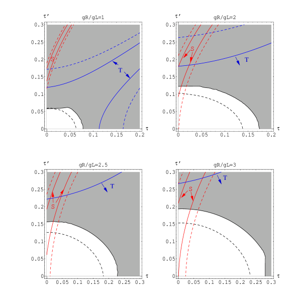
Figure 1: Combined plots of the experimental constraints on Higgsless models for different values of the $g_{5R}/g_{5L}$ ratio, in the parameter space $\tau$–$\tau^{\prime}$ (normalized by $R\log R^{\prime}/R$). The solid contours for $S$ (red) and $T$ (blue) are at $0.25$; the dashed contours at $0.5$. The black solid (dashed) line corresponds to a deviation in the differential cross section of $3\%$ ($2\%$) at LEP2. The shaded region is excluded by a deviation larger that $3\%$ at LEP and/or direct search at Run1 at Tevatron.

3.2 Delocalized Reference Fermions

In the following, we would like to focus on an alternative solution to the $S$ problem which has additional beneficial side-effects. It has been known for a long time in Randall-Sundrum (RS) models with a Higgs that the effective $S$ parameter is large and negative [29] if the fermions are localized on the TeV brane as originally proposed [2]. When the fermions are localized on the Planck brane the contribution to $S$ is positive, and so for some intermediate localization the $S$ parameter vanishes, as first pointed out for RS models by Agashe et al.[12]. The reason for this is fairly simple. Since the $W$ and $Z$ wavefunctions are approximately flat, and the gauge KK mode wavefunctions are orthogonal to them, when the fermion wavefunctions are also approximately flat the overlap of a gauge KK mode with two fermions will approximately vanish. Since it is the coupling of the gauge KK modes to the fermions that induces a shift in the $S$ parameter, for approximately flat fermion wavefunctions the $S$ parameter must be small. Note that not only does reducing the coupling to gauge KK modes reduce the $S$ parameter, it also weakens the experimental constraints on the existence of light KK modes. This case of delocalized bulk fermions is not covered by the no–go theorem of [17], since there it was assumed that the fermions are localized on the Planck brane.

In order to quantify these statements, it is sufficient to consider a toy model where all the three families of fermions are massless and have a universal delocalized profile in the bulk. We first briefly review the bulk equation of motion in AdS₅. In 5D fermions are vector-like, so that they contain both a left- and right-handed component:

$$\Psi=\left(\begin{array}[]{c}\chi\\ {\psi}\end{array}\right)~{},$$ (3.4)

where the boundary conditions can be chosen such that there is a zero mode either in the left–handed (lh) or in the right–handed (rh) component. Taking into account the AdS₅ metric and spin connection [10], the bulk Lagrangian is the following:

$$S=\int d^{5}x\left(\frac{R}{z}\right)^{4}\left(-i\bar{\chi}\bar{\sigma}^{\mu}\partial_{\mu}\chi-i\psi\sigma^{\mu}\partial_{\mu}\bar{\psi}+{\textstyle\frac{1}{2}}(\psi\overleftrightarrow{\partial_{z}}\chi-\bar{\chi}\overleftrightarrow{\partial_{z}}\bar{\psi})+\frac{c}{z}\left(\psi\chi+\bar{\chi}\bar{\psi}\right)\right),$$ (3.5)

where $c$ is a bulk Dirac mass in unit of the AdS curvature $1/R$. The bulk equations of motion derived from this action are:

$$-i\bar{\sigma}^{\mu}\partial_{\mu}\chi-\partial_{z}\bar{\psi}+\frac{c+2}{z}\bar{\psi}=0,$$ (3.6)

$$-i\sigma^{\mu}\partial_{\mu}\bar{\psi}+\partial_{z}\chi+\frac{c-2}{z}\chi=0.$$ (3.7)

If the zero mode is lh, the solution is the following:

$$\chi_{0}=A_{0}\left(\frac{z}{R}\right)^{2-c_{L}},$$ (3.8)

where the normalization is fixed by the condition

$$\int_{R}^{R^{\prime}}dz\left(\frac{R}{z}\right)^{5}\frac{z}{R}\,A_{0}^{2}\left(\frac{z}{R}\right)^{4-2c_{L}}=1\,,\ \ i.e.\ \ A_{0}=\frac{\sqrt{1-2c_{L}}}{R^{c_{L}}\sqrt{R^{\prime\,1-2c_{L}}-R^{1-2c_{L}}}}~{}.$$ (3.9)

A similar result applies for rh solutions, where $c_{L}$ is replaced by $-c_{R}$. Studying the above profile, it’s easy to show that lh (rh) fermions are localized on the Planck brane if $c_{L}>1/2$ ($c_{R}<-1/2$), else on the TeV brane, while for $c_{L}=1/2$ ($c_{R}=-1/2$) the profile is flat.

Now, the gauge couplings of the fermions will depend on the parameter $c$ through the bulk integral of the gauge boson wave functions. For a lh fermion, that transforms under the bulk gauge group as a $2_{L}\times 1_{R}\times q_{B-L}$ representation, it reads:

$$a_{0}\,Q\,\gamma_{\mu}+g_{5L}\,\mathcal{I}_{l}^{L\mp}(c_{L})\,T_{L\pm}W^{\mp}_{\mu}+g_{5L}\,\mathcal{I}_{l}^{(L3)}(c_{L})\,\left(T_{L3}+\frac{\tilde{g}_{5}\,\mathcal{I}_{l}^{(B)}(c_{L})}{g_{5L}\,\mathcal{I}_{l}^{(L3)}(c_{L})}\,\frac{Y}{2}\right)Z_{\mu}~{},$$ (3.10)

where we have used that $Y/2=Q_{B-L}$ (for $SU(2)_{R}$ singlets) and the electric charge is defined as $Q=Y/2+T_{L3}$, and:

$$\mathcal{I}^{X}_{l}(c)=A_{0}^{2}\,\int_{R}^{R^{\prime}}dz\left(\frac{R}{z}\right)^{2\,c}\,\phi_{1}^{X}(z)~{}.$$ (3.11)

Here, following the notation in [15], $a_{0}$ is the photon wave function, while $\phi_{1}^{X}(z)$ are the $W$ or $Z$ profiles.

Eq. (3.10) is a generalization of eq. (3.1) in [15], where the value of the gauge boson wave functions on the Planck brane is replaced by the bulk integral, weighted by the fermion profile squared. Only the electric charge does not depend on the fermion profile, as the massless photon is flat along the extra dimension. However, such corrections to the gauge couplings are universal, so they can be cast into the definition of the oblique parameters and yield an effective shift of $S$, $T$ and $U$.

In order to do that, we have to impose the following matching condition between the 4D couplings and the 5D parameters of the theory:

$$\tan^{2}\theta_{W}=\frac{{g^{\prime}}^{2}}{g^{2}}=-\frac{\tilde{g}_{5}\,\mathcal{I}_{l}^{(B)}(c_{L})}{g_{5L}\,\mathcal{I}_{l}^{(L3)}(c_{L})}~{},$$ (3.12)

while the matching of the electric charge remains unaffected:

$$\frac{1}{e^{2}}=\frac{1}{a_{0}^{2}}=\left(\frac{1}{\tilde{g}_{5}^{2}}+\frac{1}{g_{5L}^{2}}+\frac{1}{g_{5R}^{2}}\right)R\log\frac{R^{\prime}}{R}~{}.$$ (3.13)

Analogously, the $W$ and $Z$ wave function normalizations are determined by the following equations:

$$g_{5L}\,\mathcal{I}_{l}^{(L\pm)}(c_{L}) = g~{},$$ (3.14)

$$g_{5L}\,\mathcal{I}_{l}^{(L3)}(c_{L}) = g\cos\theta_{W}~{}.$$ (3.15)

All the oblique corrections are now contained in the wavefunction and mass renormalizations of the gauge bosons.

For a rh fermion, that transforms as $1_{L}\times 2_{R}\times q_{B-L}$, the situation is a little bit more complicated. The gauge couplings are the following:

$$a_{0}\,Q\,\gamma_{\mu}+\tilde{g}_{5}\,\mathcal{I}_{r}^{B}(c_{R})\,\frac{Y}{2}Z_{\mu}+g_{5R}\,\mathcal{I}_{r}^{R\mp}(c_{R})\,T_{R\pm}W^{\mp}_{\mu}+\left(g_{5R}\,\mathcal{I}_{r}^{(R3)}(c_{R})-\tilde{g}_{5}\,\mathcal{I}_{r}^{(B)}(c_{R})\right)\,T_{R3}Z_{\mu}~{},$$ (3.16)

where

$$\mathcal{I}^{X}_{r}(c)=\mathcal{I}^{X}_{l}(-c)~{}.$$ (3.17)

In the simple case where $c_{R}=-c_{L}$, the first two terms of eq. (3.16) match the SM gauge couplings as defined above. However, the two additional terms vanish on the Planck brane only, due to the boundary conditions. In general they will give rise to non-oblique corrections (see sec. 5.2).

The computation of the oblique corrections follows straightforwardly from the matching conditions (3.12) and (3.13). Before showing some numerical results, it is useful to understand the analytical behavior of $S$ in interesting limits. For fermions almost localized on the Planck brane, it is possible to expand the result in powers of $(R/R^{\prime})^{2c_{L}-1}\ll 1$. The leading terms, also expanding in powers of $1/\log$, are:

$$S=\frac{6\pi}{g^{2}\,\log\frac{R^{\prime}}{R}}\left(1-\frac{4}{3}\frac{2c_{L}-1}{3-2c_{L}}\left(\frac{R}{R^{\prime}}\right)^{2c_{L}-1}\log\frac{R^{\prime}}{R}\right)~{},$$ (3.18)

and $U\approx T\approx 0$. The above formula is actually valid for $1/2<c_{L}<3/2$. For $c_{L}>3/2$ the corrections are of order $(R^{\prime}/R)^{2}$ and numerically negligible. As we can see, as soon as the fermion wave function starts leaking into the bulk, $S$ decreases.

Another interesting limit is when the profile is almost flat, $c_{L}\approx 1/2$. In this case, the leading contributions to $S$ are:

$$S=\frac{2\pi}{g^{2}\,\log\frac{R^{\prime}}{R}}\left(1+(2c_{L}-1)\,\log\frac{R^{\prime}}{R}+\mathcal{O}\left((2c_{L}-1)^{2}\right)\right)~{}.$$ (3.19)

In the flat limit $c_{L}=1/2$, $S$ is already suppressed by a factor of 3 with respect to the Planck brane localization case. Moreover, the leading terms cancel out for:

$$c_{L}=\frac{1}{2}-\frac{1}{2\,\log\frac{R^{\prime}}{R}}\approx 0.487~{}.$$ (3.20)

For $c_{L}<1/2$, $S$ becomes large and negative and, in the limit of TeV brane localized fermions ($c_{L}\ll 1/2$):

$$S=-\frac{16\pi}{g^{2}}\frac{1-2c_{L}}{5-2c_{L}}~{},$$ (3.21)

while, in the limit $c_{L}\rightarrow-\infty$:

$$T \rightarrow \frac{2\pi}{g^{2}\,\log\frac{R^{\prime}}{R}}(1+\tan^{2}\theta_{W})\approx 0.5~{},$$ (3.22)

$$U \rightarrow -\frac{8\pi}{g^{2}\,\log\frac{R^{\prime}}{R}}\frac{\tan^{2}\theta_{W}}{2+\tan^{2}\theta_{W}}\frac{1}{c_{L}}\approx 0~{}.$$ (3.23)

Figure 2: Plots of the oblique parameters as function of the bulk mass of the reference fermion. The values on the right correspond to localization on the Planck brane. $S$ vanishes for $c=0.487$.

In Fig. 2 we show the numerical results for the oblique parameters as function of $c_{L}$. We can see that, after vanishing for $c_{L}\approx 1/2$, $S$ becomes negative and large, while $T$ and $U$ remain smaller.

4 Perturbative Unitarity

The other criticism leveled at Higgsless models is that if the KK modes are above $1$ TeV then perturbative unitarity might break down near $2$ TeV, thus rendering perturbative calculations impossible. If this were the case then Higgsless theories would look very much like technicolor theories and it would be difficult to make any theoretical progress.

The amplitude of elastic scattering of longitudinal massive $W$ blows up at around $1.8$ TeV, thus violating perturbative unitarity. In the SM it is restored by the contribution of the Higgs field, that cancels the residual term growing with the energy squared. As is by now well known, in Higgsless models perturbative unitarity breakdown is delayed by the contribution of the KK modes of ordinary gauge bosons [6]: as a consequence of 5D gauge invariance, two sum rules involving trilinear gauge couplings and masses ensure the cancellation of the terms growing like $E^{4}$ and $E^{2}$. This implies a first constraint on the spectrum. Over large regions of the parameter space the sum rules are very accurately satisfied with only the first two KK modes, which typically happens when masses stay below $1500$ GeV.

Even though the growing terms are tamed, it is still possible for the tree–level elastic scattering amplitude to break down around $2-3$ TeV in Higgsless theories [13, 16]. However, this residual growth is due to the presence of large logarithms coming from the forward scattering region, after integrating over the scattering angle. Such logarithms are present in the SM as well (in particular from the t-channel photon exchange, whose contribution is divergent), but in our case they are enhanced by a large coefficient growing with the resonance mass. The log term in the s–partial wave amplitude is given by:

$$\frac{g_{WWZ_{k}}^{2}}{32\pi}\left(2-\frac{M_{Z_{k}}^{2}}{M_{W}^{2}}\right)^{2}\log\left(\frac{4E^{2}}{M_{Z_{k}}^{2}}\right)~{}.$$ (4.1)

Such behavior is not particular to Higgsless theories and can be easily reproduced in simple 4D toy models. In this case however they are unphysical: they arise when the energy is much larger than the resonance mass, where other inelastic channels open up and cannot be neglected in the unitarization of the $S$ matrix [26]. Thus, the spoiling of partial wave unitarity, if due to such large logs, cannot indicate the scale where a strong coupling regime is entered.

On the other hand, from a 5D point of view a linear growth of the amplitude is expected. Indeed, according to naive dimensional analysis (NDA), the loop factor grows with the energy as

$$\frac{g_{5}^{2}}{24\pi^{3}}E\,.$$ (4.2)

From the strength of this loop factor, warped down to the TeV scale, we conclude that perturbativity breaks down around a scale

$$\Lambda_{\rm NDA}\sim\frac{24\pi^{3}}{g_{5}^{2}}\frac{R}{R^{\prime}}\,.$$ (4.3)

In the warped Higgsless model, the NDA cutoff scale can be expressed in terms of the masses of the $W$ and the first KK excitation and the 4D SM gauge coupling:

$$\Lambda_{\rm NDA}\sim\frac{12\pi^{4}M_{W}^{2}}{g^{2}M_{W^{(1)}}}\,.$$ (4.4)

From the formula above, it is clear that the heavier the resonance, the lower the scale where perturbative unitarity gets lost. This also gives a rough estimate, valid up to a numerical coefficient, of the actual scale of non–perturbative physics. An explicit calculation of the scattering amplitude, including inelastic channels, shows that this is indeed the case and the numerical factor is found to be roughly $1/4$ [26].

Since the ratio of the $W$ to the first KK mode mass squared is of order

$$\frac{M_{W}^{2}}{M_{W^{(1)}}^{2}}=\mathcal{O}\left({1}/{\log\left({R^{\prime}}/{R}\right)}\right)~{},$$ (4.5)

raising the value of $R$ (corresponding to lowering the 5D UV scale) will significantly increase the NDA cutoff. With $R$ chosen to be the inverse Planck scale, the first KK resonance appears around $1.2$ TeV, but for larger values of $R$ this scale can be safely reduced down below a TeV. As already discussed in the previous section, such resonances will be weakly coupled to almost flat fermions and can easily avoid the strong bounds from direct searches at LEP or Tevatron. If we are imagining that the AdS space is a dual description of an approximate conformal field theory (CFT), then $1/R$ is the scale where the CFT is no longer approximately conformal and perhaps becomes asymptotically free. Thus it is quite reasonable that the scale $1/R$ would be much smaller than the Planck scale.

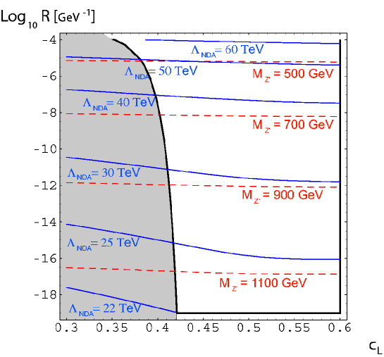
Figure 3: Contour plots of $\Lambda_{\rm NDA}$ (solid blue lines) and $M_{Z^{(1)}}$ (dashed red lines) in the parameter space $c_{L}$–$R$. The shaded region is excluded by direct searches of light $Z^{\prime}$ at LEP.

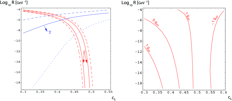
Figure 4: On the left, contours of $S$ (red), for $|S|=0.25$ (solid) and $0.5$ (dashed) and $T$ (blue), for $|T|=0.1$ (dotted), $0.3$ (solid) and $0.5$ (dashed), as function of $c_{L}$ and $R$. On the right, contours for the generic suppression of fermion couplings to the first resonance with respect to the SM value. In particular we plotted the couplings of a lh down–type massless quark with the $Z^{\prime}$. The region for $c_{L}$, allowed by $S$, is between $0.43\div 0.5$, where the couplings are suppressed at least by a factor of 10.

In Fig. 3 we have plotted the value of the NDA scale (4.3) as well as the mass of the first resonance in the $(c_{L}-R)$ plane. Increasing $R$ also affects the oblique corrections. However, while it is always possible to reduce $S$ by delocalizing the fermions, $T$ increases and puts a limit on how far $R$ can be raised. One can also see form Fig. 4 that in the region where $|S|<0.25$, the coupling of the first resonance with the light fermions is generically suppressed to less than $10\%$ of the SM value. This means that the LEP bound of $2$ TeV for SM–like $Z^{\prime}$ is also decreased by a factor of 10 at least (the correction to the differential cross section is roughly proportional to $g^{2}/M_{Z^{\prime}}^{2}$). In the end, values of $R$ as large as $10^{-7}$ GeV^-1 are allowed, where the resonance masses are around $600$ GeV. So, even if, following the analysis of [26], we take into account a factor of roughly $1/4$ in the NDA scale, we see that the appearance of strong coupling regime can be delayed up to $10$ TeV. At the LHC it will be very difficult to probe $WW$ scattering above 3 TeV.

5 Flavor Physics

As already mentioned, fermions masses can be easily reproduced by boundary conditions [10]. Since they must be bulk fields in a Higgsless model (otherwise it would not be possible to produce a isospin breaking mass spectrum for them), and since in 5D the smallest representation of the Lorentz group is a Dirac spinor, one is forced to introduce a full Dirac spinor for every SM field. For the third generation quarks for example this implies that one has at least the fields

$$\left(\begin{array}[]{c}\chi_{tL}\\ {\psi}_{tL}\\ \chi_{bL}\\ {\psi}_{bL}\end{array}\right)\ \ \ \left(\begin{array}[]{c}\chi_{tR}\\ {\psi}_{tR}\\ \chi_{bR}\\ {\psi}_{bR}\end{array}\right),$$ (5.1)

where the $\psi$’s are right handed 4D Weyl spinors, while the $\chi$’s are left handed 4D Weyl spinors, and the subscript $L,R$ denote whether these fields are part of the $SU(2)_{L}$ or $SU(2)_{R}$ doublet. In order to get the correct spectrum, one needs to make sure that the boundary conditions of the $L$ and $R$ fields are different, for example by imposing $(+,+)$ boundary conditions on the $\chi_{tL,bL}$ and $\psi_{tR,bR}$ fields, in order to obtain approximate zero modes, and consequently applying the opposite $(-,-)$ boundary conditions to the remaining fields.

An acceptable mass spectrum can then be generated by noting that the gauge group on the TeV brane is non-chiral, and therefore a Dirac mass

$$M_{D}R^{\prime}(\chi_{tL}\psi_{tR}+\chi_{bL}\psi_{bR})$$ (5.2)

can be added on the TeV brane. Due to the remaining $SU(2)_{D}$ gauge symmetry the same term has to be added for top and bottom quarks. The necessary splitting between top and bottom can then be achieved by adding a large brane induced kinetic term for $\psi_{bR}$ on the Planck brane (where $SU(2)_{R}$ is broken) [9]. This is equivalent to adding a mixing on the Planck brane to a localized singlet field, that we parametrize by the ratio $\xi$ between the mixing mass and the mass of the localized field [7, 10].

In the following subsections we will address some issues about flavor physics arising in this scenario. First of all, the eventual presence of flavor changing neutral currents (FCNC) induced either by higher dimension operators or by non–universal corrections. Next, we will briefly discuss the problems surrounding the inclusion of the third family of quarks in the picture. For interesting flavor physics signals in warped extra dimensional models see [34].

5.1 FCNC from higher order operators

In a warped background, the scale suppressing dimensionful operators depends on the position of the fields along the extra-dimension [35]: for operators involving fields mostly localized on the UV brane, the suppression scale will be approximately $1/R$, while for operators with fields localized on the IR brane, the scale will rather be around $1/R^{\prime}$. There are severe constraints on the scale of four-Fermi operators leading to FCNC, putting a lower bound around $10^{3}$ TeV. While this constraint was clearly satisfied when the two light generations of quarks and leptons were localized close to the Planck brane, it becomes more worrisome when the fermions are delocalized in the bulk, a situation favored as we have just seen by electroweak precision measurements.

Let us for instance consider the 5D operator

$$\int d^{5}x\left(\frac{R}{z}\right)^{5}\,R^{3}\ \bar{\Psi}_{L}\Gamma^{M}\Psi_{L}\ \bar{\Psi}_{L}\Gamma_{M}\Psi_{L}$$ (5.3)

where $\Gamma^{M}$ are the 5D Dirac matrices (see for instance app. A of [10]) and where $\Psi_{L}$ is the 5D SU(2)_L doublet of the first (or second) generation of quarks and containing in particular the $u_{L}$ and $d_{L}$ zero modes. Note that the scale suppressing this 5D operator is set by the 5D UV cutoff $1/R$. Upon compactification, this operator will in particular generate the 4D FCNC operator

$$\int d^{4}x\ \frac{1}{\Lambda_{FCNC}^{2}}\ \bar{\chi}_{u_{L}}\gamma^{\mu}\chi_{u_{L}}\ \bar{\chi}_{d_{L}}\gamma_{\mu}\chi_{d_{L}}$$ (5.4)

where the scale $\Lambda_{FCNC}$ is obtained from eq. (5.3) after integration of the fermion zero-mode profiles over the extra-dimension. For $c_{L}\approx 1/2$, we get:

$$\Lambda_{FCNC}^{2}\approx\frac{(R/R^{\prime})^{2-4c_{L}}\log(R^{\prime}/R)}{R^{\prime 2}}.$$ (5.5)

For $1/R^{\prime}\sim 1$ TeV, to get a suppression factor of $10^{3}$ TeV, $c_{L}$ would have to be bigger than $0.57$. Clearly the values of $c_{L}$ used to reduce the $S$ parameter do not fulfill this criterion, which means that the set-up fails to naturally explain the absence of FCNC and additional flavor symmetries in 5D would be necessary. It is however relatively easy to impose such a flavor symmetry in the bulk and on the TeV brane and naturally break it close to the Planck brane. Due to the small overlap of the fermion wavefunctions on the Planck brane, the suppression scale of the four-Fermi operators will be significantly increased.

Finally let us mention that other 5D operators like

$$\int d^{5}x\left(\frac{R}{z}\right)^{5}\,R^{3}\ \bar{\Psi}_{L}\Psi_{R}\ \bar{\Psi}_{R}\Psi_{L}$$ (5.6)

that would lead to the 4D operator

$$\int d^{4}x\ \frac{1}{\Lambda_{FCNC}^{2}}\ \chi_{u_{L}}\psi_{d_{R}}\ \psi_{d_{R}}\chi_{u_{L}}$$ (5.7)

are less constraining since the suppression scale $\Lambda_{FCNC}$ can be now raised by localizing the rh components of the fermion on Planck brane ($c_{R}<-1/2$), as discussed in sec. 5.2. Thus for these operators $\Lambda_{FCNC}$ can be as high as $10^{3}$ TeV even if $c_{L}<1/2$.

5.2 Non–oblique Corrections: Light Fermions.

Due to fermions propagating into the bulk, the model is also affected by corrections to the gauge couplings that cannot be removed by a shift of the oblique parameters. There are two types of such corrections: corrections coming from the enlarged gauge structure in the bulk (already mentioned in sec. 3.2), and non–universal corrections coming from the different fermion masses. We can parametrize the combination of these corrections as shifts with respect to the SM couplings, as follows:

$$\begin{array}[]{lcl}g^{Z}_{f_{l}}=\left(1+\gamma_{l}^{f}\right)\frac{g}{\cos\theta_{W}}\left(T_{3}+\sin^{2}\theta_{W}\,Q\right)\,,&&g^{W}_{f_{l}}=\left(1+\omega_{l}^{f}\right)g\,,\\ g^{Z}_{f_{r}}=\left(1+\gamma_{r}^{f}\right)g^{\prime}\sin\theta_{W}\,Q\,,&&g^{W}_{f_{r}}=\omega_{r}^{f}g\,.\end{array}$$ (5.10)

The corrections arising from the enlarged gauge structure affect the couplings of the rh fermions. They are present in the massless limit, and are universal provided that the bulk masses of the $SU(2)_{R}$ doublets, $c_{R}$, are all equal. These corrections are generically not very tightly bounded by experiment. For example, from the $\mu$ decay the limits on the $W$ couplings with rh electron and muon, $\omega_{r}^{e,\,\mu}$, is of order few % with respect to the SM gauge coupling, while from the $\tau$ leptonic decays $\omega_{r}^{\tau}$ has to be smaller than 10% [36].

On the other hand, boundary conditions generating fermion masses distort the zero mode profiles, introducing non-universal corrections to the gauge couplings. The more the fermion probes the bulk, the more severe such non–universalities are, as the wave function will be more sensitive to the TeV-localized mass term. For the first generation, the corrections given by the masses (much smaller than the electroweak scale) are negligible. Nevertheless, there are non–oblique corrections that generically will be $\gamma_{l}\approx\omega_{r}\approx\mbox{few}\cdot 10^{-4}$ for $c_{R}<-1/2$.

The most stringent experimental constraints come from non–universalities between the first two generations of quarks, for example $\delta\gamma^{ds}_{l}=\gamma_{l}^{s}-\gamma_{l}^{d}$ and $\delta\gamma^{ds}_{r}=\gamma_{r}^{s}-\gamma_{r}^{d}$ from Kaon physics [37]. The bounds generically imply $|\delta\gamma^{ds}|<10^{-5}$. Weaker bounds also come from $B^{0}$–$\bar{B}^{0}$ and $D^{0}$–$\bar{D}^{0}$ mixings, namely $|\delta\gamma^{cu}|<10^{-4}$ and $|\delta\gamma^{bd}|<5\cdot 10^{-4}$. Such bounds depend on unknown quark mixing matrices, so can be weaker if small elements are involved (see [37] for more details). It is possible, however, to tune $c_{L}$ and $c_{R}$ for the second generation in order to fulfill such bounds. A numerical example is shown in table 1, in the minimal scenario where only a localized kinetic term is added to the R-component of the lighter quark. In this example $\gamma_{r}^{c}$ is too large. It is however easy to suppress it, for example splitting the $s_{r}$ and $c_{r}$ into two different bulk $R$–doublets with different bulk masses, $c_{Rs}$ and $c_{Rc}$. Similar arguments apply to the leptons.

u	$\gamma_{l}^{u}<10^{-6}$	$\omega_{l}<10^{-6}$	$\gamma_{r}^{u}=-3.95\cdot 10^{-4}$	$\omega_{r}=1.33\cdot 10^{-5}$
d	$\gamma_{l}^{d}<10^{-6}$		$\gamma_{r}^{d}=-5.85\cdot 10^{-4}$
s	$\gamma_{l}^{s}=-8\cdot 10^{-6}$	$\omega_{l}=-5\cdot 10^{-5}$	$\gamma_{r}^{s}=-5.9\cdot 10^{-4}$	$\omega_{r}=3.8\cdot 10^{-4}$
c	$\gamma_{l}^{c}=-3.6\cdot 10^{-6}$		$\gamma_{r}^{c}=-1.5\cdot 10^{-2}$

Table 1: Parameters used in this example: $c_{L1}=0.485$, $c_{R1}=-0.6$, $M_{D1}=3.17$  GeV, $\xi_{u_{r}}=4.71$; $c_{L2}=0.485448$, $c_{R2}=-0.511$, $M_{D2}=47.5$  GeV, $\xi_{s_{r}}=59.5$; where $\xi$ is the parameter describing the localized kinetic term. In this case $\gamma_{r}^{s}-\gamma_{r}^{d}=6\cdot 10^{-6}$.

As already discussed in sec. 5.1, in the above scenario generically large FCNC are expected to arise from higher dimensional operators, as flavor symmetry is broken both by the Dirac masses on the TeV brane and by the bulk masses. An elegant way out is to impose a bulk flavor symmetry, and exile all the flavor structure on the Planck brane. In this case, higher dimensional operators will be generically safely suppressed by the scale $1/R$. In a minimal scenario, one can add a universal Dirac mass for quarks (and another for leptons) in order to account for the heaviest particle (charm or $\tau$). Then the lighter masses are suppressed by localized kinetic terms for the $L$–doublet and the two singlets on the Planck brane.

5.3 Top mass, $Zb\bar{b}$ coupling and loop induced isospin violations

The major challenge facing Higgsless models is the incorporation of the third family of quarks. There is a tension [14, 12] in obtaining a large top quark mass without deviating from the observed bottom couplings with the $Z$. It can be seen in the following way. The top quark mass is proportional both to the Dirac mixing $M_{D}$ on the TeV brane and the overall scale of the extra dimension set by $1/R^{\prime}$. For $c_{L}\sim 0.5$ (or larger) it is in fact impossible to obtain a heavy enough top quark mass (at least for $g_{5R}=g_{5L}$). The reason is that for $M_{D}R^{\prime}\gg 1$ the light mode mass saturates at

$$m_{top}^{2}\sim\frac{2}{R^{\prime 2}\log\frac{R^{\prime}}{R}}\,,$$ (5.11)

which gives for this case $m_{top}\leq\sqrt{2}M_{W}$. Thus one needs to localize the top and the bottom quarks closer to the TeV brane. However, even in this case a sizable Dirac mass term on the TeV brane is needed to obtain a heavy enough top quark. The consequence of this mass term is the boundary condition for the bottom quarks

$$\chi_{bR}=M_{D}R^{\prime}\,\chi_{bL}.$$ (5.12)

This implies that if $M_{D}R^{\prime}\sim 1$ then the left handed bottom quark has a sizable component also living in an $SU(2)_{R}$ multiplet, which however has a coupling to the $Z$ that is different from the SM value. Thus there will be a large deviation in the $Zb_{L}\bar{b}_{L}$. Note, that the same deviation will not appear in the $Zb_{R}\bar{b}_{R}$ coupling, since the extra kinetic term introduced on the Planck brane to split top and bottom will imply that the right handed $b$ lives mostly in the induced fermion on the Planck brane which has the correct coupling to the $Z$.

The only way of getting around this problem would be to raise the value of $1/R^{\prime}$, and thus lower the necessary mixing on the TeV brane needed to obtain a heavy top quark. One way of raising the value of $1/R^{\prime}$ is by increasing the ratio $g_{5R}/g_{5L}$ (at the price of making also the gauge KK modes heavier and thus the theory more strongly coupled). To illustrate the magnitudes in the deviations of the $Zb_{L}\bar{b}_{L}$ coupling we have plotted the percentage variation with respect to the SM value as a function of $1/R^{\prime}$ (varying the ratio). We can see in the left hand side of Fig. 5 that the deviation decreases with increasing $1/R^{\prime}$. In order to be compatible with the experimental bound of $1\,\%$ [27] from LEP, a scale larger that $1700$ GeV is required (which implies $g_{R}/g_{L}>4.5$ and the first resonance above $4$ TeV), where the theory is already strongly coupled. On the right hand side of Fig. 5 we also show the contours of fixed amount of deviation for $g_{5R}/g_{5L}=5$.

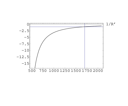
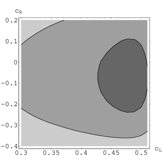
Figure 5: Plots of the percentage deviation of the $Zb_{L}\bar{b}_{L}$ coupling with respect to the SM value as function of the scale $1/R^{\prime}$ (left, with $c_{L}=0.46$ and $c_{R}=-0.05$) and as function of the bulk masses $c_{L}$ and $c_{R}$ for $1/R^{\prime}=1750$ GeV (right). The contours are at $1\,\%$ and $1.5\,\%$. Different values of $1/R^{\prime}$ are obtained varying the ratio $g_{R}/g_{L}$ between 1 and 6; the plot on the right assumes $g_{R}/g_{L}=5$.

Another generic problem arising from the large value of the top-quark mass in models with warped extra dimensions comes from the isospin violations in the KK sector of the top and the bottom quarks. If the spectrum of the top and bottom KK modes is not sufficiently degenerate, the loop corrections involving these KK modes to the $T$-parameter could be large.  This possibility was pointed out in [12], and further discussed in [38]. In [12] an estimate for the size of these loop corrections was given using a mass insertion approximation. Since the mass insertions (the Dirac mixings of the KK modes on the TeV brane) are very large, possibly larger than the unperturbed masses, this method likely gives an overestimate of the resulting T-parameter. In order to get some sense of magnitudes we nevertheless quote the results found in [12]:

$$T^{topKK}\sim 0.84\left(\frac{2}{1-2c_{L}^{top}}\right)^{2}\left(\frac{m_{t}}{m_{t}^{KK}}\right)^{2}.$$ (5.13)

For $c_{L}$ close to one half and a KK mass for the top of order 700 GeV this contribution would be enormous. One can see that in order to suppress this contribution one would again need to increase $m_{t}^{KK}$, the first KK mass of the top quark, which can only be achieved by raising the value of $1/R^{\prime}$. One would also need to move the left handed doublet closer to the TeV brane in order to reduce the $c_{L}$ dependent enhancement factor. Both this argument and the consideration of the $Zb\bar{b}$ vertex would call for a scenario where the third generation feels a different value of $R^{\prime}$ than the rest of the particles. We will speculate about such a possibility below.

5.4 Possible future directions for model building

Given that the main problem with Higgsless models arises from mass generation of the top and the consequent effects on the couplings of the $b$ quark, there are several possible directions to explore for building realistic models. A simple direction would be to relax the assumptions that the Higgs VEV is infinite and localized on the TeV brane. As long as the Higgs VEV is large compared to its SM value, its contribution to WW scattering is suppressed. A VEV above 1 TeV is probably sufficient to make its contribution at the LHC unobservably small. Once the VEV is finite it is possible to imagine the Higgs having a profile in the bulk [39] which will reduce the value of $M_{D}$ necessary in order to obtain a large mass, and thus the mixing between the $L$ and $R$ components of the lh $b$-quarks. In the dual CFT language this corresponds to the operator which breaks the electroweak symmetry having a finite scaling dimension $>2$. This is the type of dynamical breaking scenario that happens in QCD or technicolor.

A more ambitious approach would be to separate the fermion and gauge boson Higgs sectors. Conceptually we can imagine a theory with two Higgses, one of which predominantly gives mass to the gauge bosons and one which predominantly gives mass to the fermions. One could then apply the Higgs decoupling limit and arrive at a “double Higgsless” theory. More concretely we could have two AdS spaces on either side of a Planck brane, where the gauge bosons can propagate in the entire space and the fermions can only propagate in the left half. If the ratio of $g_{5R}/g_{5L}$ gauge couplings and/or the warp factor $R^{\prime}/R$ are large on the left-space then electroweak symmetry breaking on the left will contribute little to the $W$ and $Z$ gauge boson masses. This means that the gauge boson wavefunctions will be almost flat on the left. Nevertheless, $1/R^{\prime}$ can be bigger on the left, and in this way the mixing between the $L$ and $R$ components of the $b$-quark can be reduced. Also if $1/R^{\prime}$ is bigger on the left than the right then $KK$ modes of the fermions can be made heavier than the $KK$ modes of the gauge bosons, meaning that problems with Unitarity can be postponed, while suppressing isospin violating loop corrections from fermion $KK$ modes [12].

We plan to study the feasibility of such setups in the future.

6 Conclusions

There has recently been a long discussion about the feasibility of Higgsless models, when facing precision measurements. The most common criticisms are the large oblique corrections (namely, a large tree–level contribution to $S$) and a strong coupling arising from the early breakdown of partial wave unitarity in $W$ boson scattering. Due to these problems, some authors have claimed these models to be disfavored by experiment. However, we have shown that it is possible to cure these ills by delocalizing the light fermions in the bulk. In the limit of almost flat profiles, the gauge boson KK modes almost decouple from the light fermions, while remaining effective in restoring perturbative unitarity in $WW$ scattering. This yields a double advantage: the tree level contribution to $S$ is suppressed and direct search limits are lowered. Therefore, a scenario with $600$ GeV resonances and a perturbative regime up to $10$ TeV is allowed.

Finally, we pointed out that the main challenge still facing Higgsless models is actually the successful inclusion of a heavy top quark, without stumbling over large corrections to bottom couplings with the $Z$. We have also mentioned some possible future directions in model building that might lead to a completely realistic model.

References

- [1] N. Arkani-Hamed, S. Dimopoulos and G. R. Dvali, Phys. Lett. B 429, 263 (1998) hep-ph/9803315.
- [2] L. Randall and R. Sundrum, Phys. Rev. Lett. 83, 3370 (1999) hep-ph/9905221.
- [3] N. S. Manton, Nucl. Phys. B 158, 141 (1979); C. Csáki, C. Grojean and H. Murayama, Phys. Rev. D 67, 085012 (2003) hep-ph/0210133; C. A. Scrucca, M. Serone and L. Silvestrini, Nucl. Phys. B 669, 128 (2003) hep-ph/0304220; C. A. Scrucca, M. Serone, L. Silvestrini and A. Wulzer, JHEP 0402, 049 (2004) hep-th/0312267.
- [4] N. Arkani-Hamed, A. G. Cohen, E. Katz and A. E. Nelson, JHEP 0207, 034 (2002) hep-ph/0206021.
- [5] R. Harnik, G. D. Kribs, D. T. Larson and H. Murayama, Phys. Rev. D 70, 015002 (2004) hep-ph/0311349; S. Chang, C. Kilic and R. Mahbubani, hep-ph/0405267;
- [6] C. Csáki, C. Grojean, H. Murayama, L. Pilo and J. Terning, Phys. Rev. D 69, 055006 (2004) hep-ph/0305237.
- [7] C. Csáki, C. Grojean, L. Pilo and J. Terning, Phys. Rev. Lett. 92, 101802 (2004) hep-ph/0308038.
- [8] Y. Nomura, JHEP 0311, 050 (2003) hep-ph/0309189.
- [9] R. Barbieri, A. Pomarol and R. Rattazzi, Phys. Lett. B 591 (2004) 141 hep-ph/0310285.
- [10] C. Csáki, C. Grojean, J. Hubisz, Y. Shirman and J. Terning, Phys. Rev. D 70, 015012 (2004) hep-ph/0310355.
- [11] R. S. Chivukula, D. A. Dicus and H. J. He, Phys. Lett. B 525, 175 (2002) hep-ph/0111016; R. S. Chivukula and H. J. He, Phys. Lett. B 532, 121 (2002) hep-ph/0201164; R. S. Chivukula, D. A. Dicus, H. J. He and S. Nandi, hep-ph/0302263; S. De Curtis, D. Dominici and J. R. Pelaez, Phys. Lett. B 554, 164 (2003) hep-ph/0211353; Phys. Rev. D 67, 076010 (2003) hep-ph/0301059; Y. Abe, N. Haba, Y. Higashide, K. Kobayashi and M. Matsunaga, Prog. Theor. Phys. 109, 831 (2003) hep-th/0302115.
- [12] K. Agashe, A. Delgado, M. J. May and R. Sundrum, JHEP 0308, 050 (2003) hep-ph/0308036.
- [13] H. Davoudiasl, J. L. Hewett, B. Lillie and T. G. Rizzo, Phys. Rev. D 70, 015006 (2004) hep-ph/0312193.
- [14] G. Burdman and Y. Nomura, Phys. Rev. D 69, 115013 (2004) hep-ph/0312247.
- [15] G. Cacciapaglia, C. Csáki, C. Grojean and J. Terning, hep-ph/0401160.
- [16] H. Davoudiasl, J. L. Hewett, B. Lillie and T. G. Rizzo, JHEP 0405, 015 (2004) hep-ph/0403300; J. L. Hewett, B. Lillie and T. G. Rizzo, hep-ph/0407059.
- [17] R. Barbieri, A. Pomarol, R. Rattazzi and A. Strumia, hep-ph/0405040.
- [18] R. Foadi, S. Gopalakrishna and C. Schmidt, JHEP 0403, 042 (2004) hep-ph/0312324; R. Casalbuoni, S. De Curtis and D. Dominici, hep-ph/0405188.
- [19] R. S. Chivukula, E. H. Simmons, H. J. He, M. Kurachi and M. Tanabashi, hep-ph/0406077; R. S. Chivukula, H. J. He, M. Kurachi, E. H. Simmons and M. Tanabashi, hep-ph/0408262.
- [20] H. Georgi, hep-ph/0408067.
- [21] M. Perelstein, hep-ph/0408072.
- [22] T. Ohl and C. Schwinn, hep-ph/0312263; C. Schwinn, Phys. Rev. D 69, 116005 (2004) hep-ph/0402118.
- [23] J. Hirn and J. Stern, Eur. Phys. J. C 34, 447 (2004) hep-ph/0401032.
- [24] N. Evans and P. Membry, hep-ph/0406285;
- [25] S. Gabriel, S. Nandi and G. Seidl, hep-ph/0406020; T. Nagasawa and M. Sakamoto, hep-ph/0406024; C. D. Carone and J. M. Conroy, hep-ph/0407116.
- [26] M. Papucci, hep-ph/0408058.
- [27] LEP Electroweak Working Group, http://lepewwg.web.cern.ch/LEPEWWG
- [28] F. Abe et al. [CDF Collaboration], collisions Phys. Rev. Lett. 79, 2192 (1997).
- [29] C. Csáki, J. Erlich and J. Terning, Phys. Rev. D 66, 064021 (2002) hep-ph/0203034.
- [30] M. Golden and L. Randall, Nucl. Phys. B361 (1991) 3; B. Holdom and J. Terning, Phys. Lett. B247 (1990) 88. M. E. Peskin and T. Takeuchi, Phys. Rev. D 46, 381 (1992).
- [31] C. Csáki, J. Hubisz, G. D. Kribs, P. Meade and J. Terning, Phys. Rev. D 67, 115002 (2003) hep-ph/0211124; Phys. Rev. D 68, 035009 (2003) hep-ph/0303236.
- [32] K. Hagiwara et al. [Particle Data Group Collaboration], Phys. Rev. D 66, 010001 (2002).
- [33] J. Terning, Phys. Lett. B 344, 279 (1995) hep-ph/9410233.
- [34] K. Agashe, G. Perez and A. Soni, arXiv:hep-ph/0406101; arXiv:hep-ph/0408134.
- [35] T. Gherghetta and A. Pomarol, Nucl. Phys. B 586, 141 (2000) hep-ph/0003129.
- [36] S. Eidelman et al. [Particle Data Group Collaboration], Phys. Lett. B 592, 1 (2004); Particle Data Group web site http://pdg.lbl.gov.
- [37] G. Burdman, Phys. Rev. D 66, 076003 (2002), hep-ph/0205329.
- [38] K. Agashe, R. Contino and A. Pomarol, to appear; R. Contino, Cornell University seminar, March 2004; R. Contino, talk at Santa Fe 2004 workshop “Beyond the Higgs”, August 2004.
- [39] M. Luty and T. Okui, to appear.