Mesonic states and vacuum replicas in potential quark models for QCD

Abstract

In this paper, we study generic non-local NJL models for four-dimensional QCD in the limit of a large number of colours. We diagonalise, through a Bogoliubov-type transformation, the Hamiltonian of the model completely in terms of the compound operators creating/annihilating mesons — bound states of dressed quarks and antiquarks — and demonstrate a one-to-one correspondence between the Bogoliubov diagonalisation condition and the Bethe–Salpeter equation for bound states. We conclude that, in the leading order in $N_{C}$, the nontrivial contents of the theory is entirely encoded in the chiral angle — the solution to the mass-gap equation for dressed quarks. As a consequence, we extend the statement of existence of excited solutions to the mass-gap equation, called vacuum replicas, beyond the BCS level and prescribe a new index to the mesonic operators — the label of the vacuum state in which the corresponding meson is created.

I Introduction

For nearly half a century Nambu–Jona-Lasinio (NJL)NJL class of models Orsay ; Orsay2 ; Lisbon have been quite useful tools for the on going study and understanding of low-energy phenomena in QCD. Quark models with non-local quark current-current microscopic interactions, parameterised by kernels of particular forms, constitute prominent steps towards building an effective low-energy theory for the strong interactions. Besides regularising the ultraviolet divergences of the theory, these nonlocal quark kernels bring in the necessary interaction scale needed to make contact with the hadronic phenomenology. Models with quark instantaneous interaction modeled after the harmonic oscillator kernels Orsay ; Orsay2 ; Lisbon or kernels obtained in the Coulomb-gauge QCD coulg , as well as a variety of other approaches based on the linear confinement linear , constitute as many examples of closely related approaches exploiting the idea of chirally nonsymmetric solutions of a nonlinear gap equation. In this paper, we continue our studies of quark models Lisbon with instantaneous inter-quark interaction. An important feature of this class of models is the essential covariance of results and conclusions across a variety of possible forms for the confining kernel. For example, the pion-pion low-energy scattering problem can be solved in the general form, in terms of the pion mass and decay constant, regardless of the explicit form of the quark kernel, provided it is confining pipi . Another example of such universality is given by the existence of multiple chirally non-invariant solutions to the mass-gap equation, predicted in replica1 ; replica2 , found both analytically and numerically for all allowed power-like confining potentials in replica4 , and independently confirmed by calculations done in a different approach in replica3 . The same conclusion of universality holds for any low-energy phenomena considered in the framework of such class of models and, therefore, we dare to expect to be able to reproduce the low-energy properties of QCD. An important progress was achieved in 2d where a two-dimensional model for QCD tHooft in the axial gauge was considered and a second, Bogoliubov-type, transformation was performed in the mesonic sector to fully diagonalise, up to corrections of order $O(1/\sqrt{N_{C}})$, the Hamiltonian of the theory in terms of the mesonic creation/annihilation operators. The Hamiltonian approach to two-dimensional QCD in the light-cone gauge was also developed in japan . In the present paper, we extend this result to four-dimensional QCD and establish a one-to-one correspondence between the Bogoliubov condition (which ensures that the Hamiltonian is diagonalised in the mesonic sector) and the Bethe–Salpeter equation for bound quark-antiquark states. We build the corresponding amplitudes explicitly and study in detail the cases of the chiral pion and of the $\rho$-meson. We conclude that solving the Bethe–Salpeter equation in the ladder (rainbow) approximation is equivalent, in the leading order in $N_{C}$, to go beyond BCS level and to diagonalise the quartic term in the Hamiltonian of the theory. This feature is general and holds for any confining quark kernel. We use the oscillator-type quark kernel just as an example to illustrate the method. We also conclude that all the information needed for the second and final mesonic Bogoliubov transformation, is already contained in the solutions of the mass-gap equation appearing at the BCS level. Therefore, in the leading order in $N_{C}$, the chiral angle — the solution to the mass-gap equation — remains the only nontrivial characteristic of the theory and it defines the latter completely. As a result, we discuss the multiple chirally noninvariant solutions of mass-gap equations — the vacuum replicas replica1 ; replica2 ; replica4 — and conclude that, once such solutions exist, this information gets carried beyond BCS and appears as an extra spectroscopic index for mesonic states on top of the usual set $\{{\vec{P}},n,J^{PC}\}$— namely, each meson carries the following quantum numbers: the total momentum ${\vec{P}}$, the radial excitation number $n$, the $J^{PC}$ set, and, finally, the label of the vacuum state in which it is created. We discuss possible consequences of this generalisation.

The paper is organised as follows. The second section is first devoted to the diagonalisation of the Hamiltonian in the quark sector (subsection A) and then to its subsequent diagonalisation in the mesonic sector (subsection B). We end this chapter with the discussion of the equivalence between the mesonic Bogoliubov-Valatin transformation and the Bethe–Salpeter equation. Vacuum replicas are studied in the third chapter. We give the necessary details of the theory of replicas, in the first subsection, and comment on the tachyon problem, in the second subsection. Finally, in the third subsection, we generalise the theory of replicas beyond BCS and discuss the hadronic spectrum in the replica vacua. The fourth and last chapter of the paper is devoted to our conclusions and outlook.

II Diagonalisation of the quark Hamiltonian

II.1 Diagonalisation in the single-quark sector and the mass-gap equation

In this section, we give the necessary details of the quark model Orsay ; Orsay2 ; Lisbon to be used in this paper and describe the Hamiltonian diagonalisation in the single-quark sector (BCS level). Naively one should expect this to be the end of the story. However, as we shall see, the requirement of confinement, that is, no free asymptotic quarks may be allowed, will completely change this picture and we shall end up with a diagonal Hamiltonian written in terms of asymptotic mesons rather than asymptotic quarks. How this comes about will be the subject of this paper.

The Hamiltonian of the model,

$$\hat{H}=\int d^{3}x\bar{\psi}(\vec{x},t)\left(-i\vec{\gamma}\cdot\vec{\bigtriangledown}+m\right)\psi(\vec{x},t)+\frac{1}{2}\int d^{3}xd^{3}y\;J^{a}_{\mu}(\vec{x},t)K^{ab}_{\mu\nu}(\vec{x}-\vec{y})J^{b}_{\nu}(\vec{y},t),$$ (1)

contains the interaction of the quark currents $J_{\mu}^{a}(\vec{x},t)=\bar{\psi}(\vec{x},t)\gamma_{\mu}\frac{\lambda^{a}}{2}\psi(\vec{x},t)$ parameterised through the instantaneous quark kernel,

$$K^{ab}_{\mu\nu}(\vec{x}-\vec{y})=g_{\mu 0}g_{\nu 0}\delta^{ab}V_{0}(|\vec{x}-\vec{y}|).$$ (2)

In Eq. (2) we have used the simplest form of the kernel compatible with the requirement of confinement. Spatial components can be also included in the kernel (2) Lisbon . They affect, for example, the form of the mass-gap equation for the chiral angle and spin-dependent terms in the effective quark-quark interaction after a Foldy–Wounthuysen transformation (see, for example, papers hl where a heavy-light quarkonium was considered in the modified Fock-Schwinger gauge and an effective inter-quark interaction was derived).

But it is a fact, already mentioned in the introduction, that despite all the aforementioned detail variations of possible quark kernels, they all share with the kernel (2) the same low energy properties (Goldstone pion, $\pi-\pi$ Weinberg scattering lengths, Gell-Mann–Oakes–Renner formula, and so on) so that it is sufficient to stick to the form (2) as the mainstay of this work and comment on the generalisations when it is the case. Finally it is sufficient for phenomenological applications that $V_{0}(|\vec{x}|)$ should interpolate between long range confinement and short-range Coulomb behaviour. An example of such a phenomenological kernel which is able to address both, heavy-quark and light-quark limits of the theory, was considered in detail in replica1 . A pure confining kernel of the generalised power-like form,

$$V_{0}(|\vec{x}|)=K_{0}^{\alpha+1}|\vec{x}|^{\alpha},$$ (3)

with $K_{0}$ being the mass parameter, was studied for the first time, in the series of papers Orsay and an analysis was performed concerning the general properties of the mass-gap equations for such potentials. This analysis was extended in a recent paper replica4 and the range of possible powers $\alpha$ was identified to be $0\leqslant\alpha\leqslant 2$. In what follows, we do not need to specify any particular form for $V_{0}(|\vec{x}|)$ other than requiring it to be confining. When needed, we shall use the oscillator-type quark kernel corresponding to the case of $\alpha=2$ in Eq. (3), to exemplify some general results. Convenience of such a choice follows from the fact that the Fourier transform of the potential $\vec{x}^{2}$ is given by the Laplacian of the three-dimensional delta function, so that all integral equations can be transformed into differential equations which are much easier for analytical and numerical studies Orsay ; Orsay2 ; Lisbon .

Now we proceed in the standard way by defining dressed quarks with the help of a Bogoliubov-Valatin transformation having the chiral angle $\varphi(p)\equiv\varphi_{p}$ Orsay ; Lisbon as a parameter:

$$\psi_{\alpha}(\vec{x},t)=\sum_{s=\uparrow,\downarrow}\int\frac{d^{3}p}{(2\pi)^{3}}e^{i\vec{p}\vec{x}}[\hat{b}_{\alpha s}(\vec{p},t)u_{s}(\vec{p})+\hat{d}_{\alpha s}^{\dagger}(-\vec{p},t)v_{s}(-\vec{p})],$$ (4)

$$\left\{\begin{array}[]{rcl}u(\vec{p})&=&\frac{1}{\sqrt{2}}\left[\sqrt{1+\sin\varphi_{p}}+\sqrt{1-\sin\varphi_{p}}\;(\vec{\alpha}\hat{\vec{p}})\right]u(0),\\ v(-\vec{p})&=&\frac{1}{\sqrt{2}}\left[\sqrt{1+\sin\varphi_{p}}-\sqrt{1-\sin\varphi_{p}}\;(\vec{\alpha}\hat{\vec{p}})\right]v(0),\end{array}\right.$$ (5)

$$\hat{b}_{s}(\vec{p},t)=e^{iE_{p}t}\hat{b}_{s}(\vec{p},0),\quad\hat{d}_{s}(-\vec{p},t)=e^{iE_{p}t}\hat{d}_{s}(-\vec{p},0),$$ (6)

where $E_{p}$ stands for the dispersive law of the dressed quarks; $\alpha$ being the colour index, $\alpha=\overline{1,N_{C}}$. It is convenient to define the chiral angle varying in the range $-\frac{\pi}{2}<\varphi_{p}\leqslant\frac{\pi}{2}$ with the boundary conditions $\varphi(0)=\frac{\pi}{2}$, $\varphi(p\to\infty)\to 0$. Notice that this definition is not unique and in some cases one is forced to choose $\varphi(0)=-\frac{\pi}{2}$, as we shall see.

The normal ordered Hamiltonian (1) can be split into three parts,

$$\hat{H}=E_{\rm vac}+:\hat{H}_{2}:+:\hat{H}_{4}:,$$ (7)

and the usual procedure is to demand the quadratic part $:\hat{H}_{2}:$ to be diagonal or, equivalently, that the vacuum energy $E_{\rm vac}$ should become a minimum. Then, the corresponding mass-gap equation ensures the anomalous Bogoliubov terms $\hat{b}^{\dagger}\hat{d}^{\dagger}-\hat{d}\hat{b}$ to be absent in $:\hat{H}_{2}:$,

$$A_{p}\cos\varphi_{p}-B_{p}\sin\varphi_{p}=0,$$ (8)

where

$$A_{p}=m+\frac{1}{2}C_{F}\int\frac{d^{3}k}{(2\pi)^{3}}V_{0}(\vec{p}-\vec{k})\sin\varphi_{k},$$ (9)

$$B_{p}=p+\frac{1}{2}C_{F}\int\frac{d^{3}k}{(2\pi)^{3}}\;(\hat{\vec{p}}\hat{\vec{k}})V_{0}(\vec{p}-\vec{k})\cos\varphi_{k},$$ (10)

$C_{F}=\frac{1}{2}(N_{C}-1/N_{C})$ being the $SU(N_{C})_{C}$ Casimir operator in the fundamental representation. The large-$N_{C}$ limit implies that the product $C_{F}V_{0}$ remains finite as $N_{C}\to\infty$, so that, for the power-like form (3), an appropriate rescaling of the potential strength $K_{0}$ is understood. In the remainder of this paper we shall absorb the coefficient $C_{F}$ into the definition of the potential, $C_{F}V_{0}(|\vec{x}|)\equiv V(|\vec{x}|)$ by a trivial redefinition of $K_{0}$.

As soon as the mass-gap equation is solved and a nontrivial chiral angle is found, the Hamiltonian (7) takes a diagonal form,

$$\hat{H}=E_{\rm vac}+\sum_{\alpha}\sum_{s=\uparrow,\downarrow}\int\frac{d^{3}p}{(2\pi)^{3}}E_{p}[\hat{b}^{\dagger}_{\alpha s}(\vec{p})\hat{b}_{\alpha s}(\vec{p})+\hat{d}^{\dagger}_{\alpha s}(-\vec{p})\hat{d}_{\alpha s}(-\vec{p})],$$ (11)

and the contribution of the $:\hat{H}_{4}:$ part is suppressed as $1/\sqrt{N_{C}}$. The dressed quark dispersive law becomes

$$E_{p}=A_{p}\sin\varphi_{p}+B_{p}\cos\varphi_{p},$$ (12)

and this completes the diagonalisation of the Hamiltonian in the quark sector to order $1/\sqrt{N_{C}}$ (the BCS level).

For further convenience we write out both the mass-gap equation and the dressed quark dispersive law $E_{p}$ for the harmonic oscillator potential, $V(|\vec{x}|)=K_{0}^{3}|\vec{x}|^{2}$ Orsay ; Orsay2 ; Lisbon ,

$$p^{3}\sin\varphi_{p}=\frac{1}{2}K_{0}^{3}\left[p^{2}\varphi^{\prime\prime}_{p}+2p\varphi_{p}^{\prime}+\sin 2\varphi_{p}\right]+mp^{2}\cos\varphi_{p},$$ (13)

$$E_{p}=m\sin\varphi_{p}+p\cos\varphi_{p}-K_{0}^{3}\left[\frac{{\varphi^{\prime}_{p}}^{2}}{2}+\frac{\cos^{2}\varphi_{p}}{p^{2}}\right].$$ (14)

In the remainder of this subsection, if not stated otherwise, we consider the chiral limit $m=0$.

We end this introductory section by stating two general properties held by mass-gap equations, Eq. (8). First of all, notice that using the explicit form of the dressed quark dispersive law $E_{p}$ (14), the mass-gap equation (13) can be rewritten in the form of a Schrödinger-like equation with the zero eigenvalue,

$$[-K_{0}^{3}\Delta_{p}+2E_{p}]\psi=0,$$ (15)

where $\psi\equiv\sin\varphi_{p}$. The generic mass-gap equation (8) for an arbitrary power-like confining potential (3) admits the form similar to (15) replica4 .

The second general property concerns the asymptotic behaviour of the solutions of the mass gap equation (the chiral angle) at large momenta. Taking the general form of the mass-gap equation for the power-like potential (3) replica4 ,

$$p^{3}\sin\varphi_{p}=K_{0}^{\alpha+1}\Gamma(\alpha+1)\sin\frac{\pi\alpha}{2}\int_{-\infty}^{\infty}\frac{dk}{2\pi}\left\{\frac{pk\sin[\varphi_{k}-\varphi_{p}]}{|p-k|^{\alpha+1}}+\frac{\cos\varphi_{k}\sin\varphi_{p}}{(\alpha-1)|p-k|^{\alpha-1}}\right\},$$ (16)

and performing an expansion for $p\to\infty$, we get

$$\left.\varphi_{p}\right|_{m=0}\mathop{\approx}\limits_{p\to\infty}-\frac{\pi}{N_{C}}\Gamma(\alpha+2)K_{0}^{\alpha+1}\sin\frac{\pi\alpha}{2}\frac{\langle\bar{q}q\rangle}{p^{\alpha+4}}.$$ (17)

From the behaviour (17) we see that, in the chiral limit, the sign of the solution $\varphi_{p}$ at large momenta is opposite to the sign of the chiral condensate. Beyond the chiral limit the expression (17) defines how the chiral angle approaches the free large-momentum asymptote $\arctan\frac{m}{p}$. From the Gell-Mann-Oakes-Renner formula GMOR one can relate the chiral condensate with the pion mass $M_{\pi}$,

$$f_{\pi}^{2}M_{\pi}^{2}=-2m\langle\bar{q}q\rangle,$$ (18)

so that, according to Eq. (17), $M_{\pi}^{2}$ becomes positive if the chiral angle approaches its large-momentum asymptote from above, and negative if it approaches from below. In the latter case the pion becomes a tachyon and this situation requires a special treatment which will be discussed in detail in chapters II and III.

II.2 Diagonalisation in the mesonic sector and the bound-state equation

II.2.1 Quark Hamiltonian in the space of quark-antiquark pairs

In this subsection, we go beyond BCS level and include the quartic part $:\hat{H}_{4}:$ of the Hamiltonian (7) into consideration.

After diagonalisation at BCS level, we could have used the formal invariance, under arbitrary Bogoliubov-Valatin transformations (BV), of the quark field $\psi_{\alpha}(\vec{x},t)$ — here understood as an inner product between a Hilbert space, spanned by the spinors $u_{s}(\vec{p})$ and $v_{s}(-\vec{p})$, and a Fock space, spanned by the quark annihilation and creation operators. This invariance requires that any given BV rotation in the Fock space, must engender a corresponding counter-rotation in the associated spinorial Hilbert space so as to maintain the inner product $\psi_{\alpha}(\vec{x},t)$ invariant. Thence, the new BV-rotated spinors will carry the information on the chiral angle and, therefore, so does the quark propagators. Equipped with these new Feynman rules, we can then proceed to evaluate a wealth of physical processes among which the Bethe-Salpeter equations for bound states play a central role. Formally, the Hamiltonian of Eq. (1), when written in terms of the quark fields $\psi_{\alpha}(\vec{x},t)$, is invariant under such BV transformations and so it will contain — through its $:\hat{H}_{4}:$ term — Bogoliubov anomalous terms of various types.

It will turn out that the set of all these Bethe-Salpeter equations, each one of them associated with a corresponding mesonic bound state, with their right mixture of positive with negative-energy amplitudes, are exactly what is required in order to get rid all the Bogoliubov anomalous terms with just four quark creation(annihilation) operators. The remaining Bogoliubov terms (responsible for generic hadronic decays like $A\to B+C$) will be suppressed as $1/\sqrt{N_{C}}$. This scenario is quite plausible once we realise that a group of four-quark creation(annihilation) operators — two quarks and two antiquarks — corresponds to a bilinear creation (annihilation) of a group of two mesons and, as we know, these bilinear anomalous terms can be made to disappear by the use of an appropriated bosonic Bogoliubov-Valatin canonical transformation.

For the implementation of the diagonalisation program we shall follow the method of refs. 2d generalising it to the four-dimensional case. The basic idea of the method is the following. At BCS level, we consider quarks as though they were free, with confinement to be implemented at later stages, when building the Bethe–Salpeter equation for bound states. Instead we now start with the ab-initio confinement requirement that only quark-antiquark pairs are allowed to be created and annihilated, not single quarks, and that the full Hamiltonian (7) must take a diagonal form in terms of the operators creating/annihilating whole quark-antiquark mesons. Therefore, every time a quark (antiquark) is created or annihilated, an accompanying antiquark (quark) must be created/annihilated as well. To write this ab-initio condition, let us introduce a set of four colourless operators: two operators which count the number of quarks and the number of antiquarks,

$$\begin{array}[]{c}\hat{B}_{ss^{\prime}}(\vec{p},\vec{p}^{\prime})=\frac{\displaystyle 1}{\displaystyle\sqrt{N_{C}}}\sum_{\alpha}\hat{b}_{\alpha s}^{\dagger}(\vec{p})\hat{b}_{\alpha s^{\prime}}(\vec{p}^{\prime}),\quad\hat{D}_{ss^{\prime}}(\vec{p},\vec{p}^{\prime})=\frac{\displaystyle 1}{\displaystyle\sqrt{N_{C}}}\sum_{\alpha}\hat{d}_{\alpha s}^{\dagger}(-\vec{p})\hat{d}_{\alpha s^{\prime}}(-\vec{p}^{\prime}),\end{array}$$ (19)

and two operators which create and annihilate a quark-antiquark pair,

$$\begin{array}[]{c}\hat{M}^{\dagger}_{ss^{\prime}}(\vec{p},\vec{p}^{\prime})=\frac{\displaystyle 1}{\displaystyle\sqrt{N_{C}}}\sum_{\alpha}\hat{b}^{\dagger}_{\alpha s^{\prime}}(\vec{p}^{\prime})\hat{d}^{\dagger}_{\alpha s}(-\vec{p}),\quad\hat{M}_{ss^{\prime}}(\vec{p},\vec{p}^{\prime})=\frac{\displaystyle 1}{\displaystyle\sqrt{N_{C}}}\sum_{\alpha}\hat{d}_{\alpha s}(-\vec{p})\hat{b}_{\alpha s^{\prime}}(\vec{p}^{\prime}).\end{array}$$ (20)

The coefficients in the definitions (19) and (20) are fixed in such a way that, in the large-$N_{C}$ limit, all four operators obey the standard bosonic algebra, with the only nonzero commutator being

$$[\hat{M}_{ss^{\prime}}(\vec{p},\vec{p}^{\prime})\;\hat{M}_{\sigma\sigma^{\prime}}^{\dagger}(\vec{q},\vec{q}^{\prime})]=(2\pi)^{3}\delta^{(3)}(\vec{p}-\vec{q})(2\pi)^{3}\delta^{(3)}(\vec{p}^{\prime}-\vec{q}^{\prime})\delta_{s\sigma}\delta_{s^{\prime}\sigma^{\prime}}.$$ (21)

The pair (19) is sufficient to express the leading part of the Hamiltonian (11),

$$\hat{H}=E_{\rm vac}+\sqrt{N_{C}}\sum_{s=\uparrow,\downarrow}\int\frac{d^{3}p}{(2\pi)^{3}}E_{p}[\hat{B}_{ss}(\vec{p},\vec{p})+\hat{D}_{ss}(\vec{p},\vec{p})],$$ (22)

whereas the suppressed part $:\hat{H}_{4}:$ requires all four operators.

According to our ab-initio confinement requirement, the operators $\hat{B}$ and $\hat{D}$ cannot be independent and have to be expressed through the operators $\hat{M}^{\dagger}$ and $\hat{M}$. One easily builds such relations to be 2d

$$\left\{\begin{array}[]{c}\hat{B}_{ss^{\prime}}(\vec{p},\vec{p}^{\prime})=\frac{\displaystyle 1}{\displaystyle\sqrt{N_{C}}}\displaystyle\sum_{s^{\prime\prime}}\int\frac{\displaystyle d^{3}p^{\prime\prime}}{\displaystyle(2\pi)^{3}}\hat{M}_{s^{\prime\prime}s}^{\dagger}(\vec{p}^{\prime\prime},\vec{p})\hat{M}_{s^{\prime\prime}s^{\prime}}(\vec{p}^{\prime\prime},\vec{p}^{\prime})\\ \hat{D}_{ss^{\prime}}(\vec{p},\vec{p}^{\prime})=\frac{\displaystyle 1}{\displaystyle\sqrt{N_{C}}}\displaystyle\sum_{s^{\prime\prime}}\int\frac{\displaystyle d^{3}p^{\prime\prime}}{\displaystyle(2\pi)^{3}}\hat{M}_{ss^{\prime\prime}}^{\dagger}(\vec{p},\vec{p}^{\prime\prime})\hat{M}_{s^{\prime}s^{\prime\prime}}(\vec{p}^{\prime},\vec{p}^{\prime\prime}).\end{array}\right.$$ (23)

The anzatz (23) is the most crucial point of the method. Formally, one can also view it as another solution to the set of equations given by the commutators of the operators (19) and (20). Notice that the relations (23) correspond to the “minimal substitution”, that is, each quark is accompanied by only one antiquark, and vice versa, whereas, in the general case, a whole quark-antiquark cloud should be also created together with the accompanying particle. Since the creation of each next quark-antiquark pair in the cloud is suppressed by an extra power of $1/N_{C}$, then Eq. (23) represents just the leading terms of the full expressions.

After substitution of the anzatz (23) into the Hamiltonian (7) we have no longer a general suppression of the quartic part of the Hamiltonian as compared to the quadratic part. Only a number of terms in $:\hat{H}_{4}:$ remain suppressed and will be omitted henceforth. The resulting Hamiltonian, in the space of colourless quark-antiquark pairs, takes the form:

$$\hat{H}=E_{\rm vac}^{\prime}+\int\frac{d^{3}P}{(2\pi)^{3}}\hat{\cal H}(\vec{P}),$$ (24)

where we have separated out the quark-antiquark cloud centre-of-mass motion.

For the sake of simplicity, let us consider the Hamiltonian density $\cal H$ at rest ($\vec{P}=0$),

$$\hat{\cal H}\equiv\hat{\cal H}(\vec{P}=0)=\sum_{s_{1}s_{2}}\int\frac{d^{3}p}{(2\pi)^{3}}2E_{p}\hat{M}_{s_{1}s_{2}}^{\dagger}(\vec{p},\vec{p})\hat{M}_{s_{2}s_{1}}(\vec{p},\vec{p})+\frac{1}{2}\sum_{s_{1}s_{2}s_{3}s_{4}}\int\frac{d^{3}p}{(2\pi)^{3}}\frac{d^{3}q}{(2\pi)^{3}}V(\vec{p}-\vec{q})$$

$$\times\left\{[v^{++}(\vec{p},\vec{q})]_{s_{1}s_{3}s_{4}s_{2}}\hat{M}^{\dagger}_{s_{2}s_{1}}(\vec{p},\vec{p})\hat{M}_{s_{4}s_{3}}(\vec{q},\vec{q})\right.+[v^{+-}(\vec{p},\vec{q})]_{s_{1}s_{3}s_{4}s_{2}}\hat{M}^{\dagger}_{s_{2}s_{1}}(\vec{q},\vec{q})\hat{M}^{\dagger}_{s_{3}s_{4}}(\vec{p},\vec{p})$$ (25)

$$\left.+[v^{-+}(\vec{p},\vec{q})]_{s_{1}s_{3}s_{4}s_{2}}\hat{M}_{s_{1}s_{2}}(\vec{p},\vec{p})\hat{M}_{s_{4}s_{3}}(\vec{q},\vec{q})+[v^{--}(\vec{p},\vec{q})]_{s_{1}s_{3}s_{4}s_{2}}\hat{M}_{s_{3}s_{4}}(\vec{p},\vec{p})\hat{M}_{s_{1}s_{2}}^{\dagger}(\vec{q},\vec{q})\right\},$$

with amplitudes $v$ given by

$$\begin{array}[]{c}[v^{++}(\vec{p},\vec{q})]_{s_{1}s_{3}s_{4}s_{2}}=[u^{\dagger}_{s_{1}}(\vec{p})u_{s_{3}}(\vec{q})][v^{\dagger}_{s_{4}}(-\vec{q})v_{s_{2}}(-\vec{p})],\\[0.0pt] [v^{+-}(\vec{p},\vec{q})]_{s_{1}s_{3}s_{4}s_{2}}=[u^{\dagger}_{s_{1}}(\vec{p})v_{s_{3}}(-\vec{q})][u^{\dagger}_{s_{4}}(\vec{q})v_{s_{2}}(-\vec{p})],\\[0.0pt] [v^{-+}(\vec{p},\vec{q})]_{s_{1}s_{3}s_{4}s_{2}}=[v^{\dagger}_{s_{1}}(-\vec{p})u_{s_{3}}(\vec{q})][v^{\dagger}_{s_{4}}(-\vec{q})u_{s_{2}}(\vec{p})],\\[0.0pt] [v^{--}(\vec{p},\vec{q})]_{s_{1}s_{3}s_{4}s_{2}}=[v^{\dagger}_{s_{1}}(-\vec{q})v_{s_{3}}(-\vec{p})][u^{\dagger}_{s_{4}}(\vec{p})u_{s_{2}}(\vec{q})].\end{array}$$ (26)

Although there are only two independent amplitudes in (26), for example, $v^{++}$ and $v^{+-}$, with the two remaining amplitudes, $v^{--}$ and $v^{-+}$, easily related to the first two by Hermitian conjugation and renaming of spin indices, we prefer to keep all four amplitudes so as to give a more symmetric form to both bound-state equations and the effective diagrammatic rules to be derived shortly.

Notice that in general, the vacuum energy in the Hamiltonian (24), $E_{\rm vac}^{\prime}$, differs from the vacuum energy $E_{\rm vac}$ in the Hamiltonian (11) by terms coming from the commutators of the operators $\hat{M}$ and $\hat{M}^{\dagger}$.

II.2.2 The case of the chiral pion

Before we proceed with the diagonalisation of the Hamiltonian (25) in general form, let us consider the case of the chiral pion as a paradigm for the general case without unnecessary complications to cloud physics. The spin and spatial structure of the pion — a ${}^{1}S_{0}$ state with $J=L=S=0$ — can be chosen in matrix form so that the operator $\hat{M}_{ss^{\prime}}(\vec{p},\vec{p})$, creating the pion at rest, is represented as

$$\hat{M}_{ss^{\prime}}(\vec{p},\vec{p})=\left[\kappa(\hat{\vec{p}})\right]_{ss^{\prime}}\hat{M}(p),\quad\kappa(\hat{\vec{p}})=\frac{i}{\sqrt{2}}\sigma_{2}Y_{00}(\hat{\vec{p}}).$$ (27)

Substitution of Eq. (27) into the Hamiltonian (25) gives a simpler expression in terms of the radial operators $\hat{M}(p)$ and $\hat{M}^{\dagger}(p)$,

$$\hat{\cal H}_{\pi}=\int\frac{p^{2}dp}{(2\pi)^{3}}2E_{p}\hat{M}^{\dagger}(p)\hat{M}(p)-\frac{1}{2}\int\frac{p^{2}dp}{(2\pi)^{3}}\frac{q^{2}dq}{(2\pi)^{3}}\left\{T^{++}_{\pi}(p,q)\hat{M}^{\dagger}(p)M(q)\right.$$

$$\left.+T^{+-}_{\pi}(p,q)\hat{M}^{\dagger}(q)\hat{M}^{\dagger}(p)+T^{-+}_{\pi}(p,q)\hat{M}(p)\hat{M}(q)+T^{--}_{\pi}(p,q)\hat{M}^{\dagger}(q)\hat{M}(p)\right\},$$ (28)

where the amplitudes $T_{\pi}^{\pm\pm}(p,q)$ are trivially built from the amplitudes $v^{\pm\pm}(\vec{p},\vec{q})$ (see Eq. (26)), after inclusion of the potential $V(\vec{p}-\vec{q})$, integration over angular variables, and taking a spin trace against the pion spin wave function $\kappa$, as it was defined in Eq. (27).

To have a fully diagonalised Hamiltonian $\hat{\cal H}_{\pi}$ it is now sufficient to perform a Bogoliubov transformation,

$$\left\{\begin{array}[]{l}\hat{M}(p)=\hat{m}_{\pi}\varphi_{\pi}^{+}(p)+\hat{m}_{\pi}^{\dagger}\varphi_{\pi}^{-}(p)\\ \hat{M}^{\dagger}(p)=\hat{m}^{\dagger}_{\pi}\varphi_{\pi}^{+}(p)+\hat{m}_{\pi}\varphi_{\pi}^{-}(p),\end{array}\right.$$ (29)

or, inversely,

$$\left\{\begin{array}[]{l}\hat{m}_{\pi}=\displaystyle\int\frac{p^{2}dp}{(2\pi)^{3}}\left[\hat{M}(p)\varphi_{\pi}^{+}(p)-\hat{M}^{\dagger}(p)\varphi_{\pi}^{-}(p)\right]\\[5.69054pt] \hat{m}_{\pi}^{\dagger}=\displaystyle\int\frac{p^{2}dp}{(2\pi)^{3}}\left[\hat{M}^{\dagger}(p)\varphi_{\pi}^{+}(p)-\hat{M}(p)\varphi_{\pi}^{-}(p)\right],\end{array}\right.$$ (30)

where the operators $\hat{m}_{\pi}^{\dagger}$ and $\hat{m}_{\pi}$ create and annihilate pions at rest.

Using the commutator of the radial operators,

$$[\hat{M}(p),\;\hat{M}^{\dagger}(q)]=\frac{(2\pi)^{3}}{p^{2}}\delta(p-q),$$ (31)

following from Eq. (21), we find that

$$[\hat{m}_{\pi},\;\hat{m}_{\pi}^{\dagger}]=\int\frac{p^{2}dp}{(2\pi)^{3}}\left[\varphi_{\pi}^{+2}(p)-\varphi_{\pi}^{-2}(p)\right].$$ (32)

Therefore, requiring the canonical commutator between the pion creation and annihilation operators to be $[m_{\pi},m_{\pi}^{\dagger}]=1$, ensures that the Bogoliubov amplitudes $\varphi_{\pi}^{\pm}$, playing the role of the pion wave functions, must in turn be subject to the normalisation

$$\int\frac{p^{2}dp}{(2\pi)^{3}}\left[\varphi_{\pi}^{+2}(p)-\varphi_{\pi}^{-2}(p)\right]=1.$$ (33)

To complete the program of bosonic diagonalisation of the Hamiltonian (1), we need only to look for a pair of $\varphi_{\pi}^{\pm}(p)$ to diagonalise the hadronic Fock subspace spanned by zero momentum pions, $|\pi_{P=0}\rangle=m^{\dagger}_{\pi}|\Omega\rangle$, $|\Omega\rangle$ being the mesonic vacuum (see the discussion below).

Now, if $\varphi_{\pi}^{+}(p)$ and $\varphi_{\pi}^{-}(p)$ are made to obey the following set of equations,

$$\left\{\begin{array}[]{l}[2E_{p}-M_{\pi}]\varphi_{\pi}^{+}(p)=\displaystyle\int\frac{\displaystyle q^{2}dq}{\displaystyle(2\pi)^{3}}[T^{++}_{\pi}(p,q)\varphi_{\pi}^{+}(q)+T^{+-}_{\pi}(p,q)\varphi_{\pi}^{-}(q)]\\[0.0pt] [2E_{p}+M_{\pi}]\varphi_{\pi}^{-}(p)=\displaystyle\int\frac{\displaystyle q^{2}dq}{\displaystyle(2\pi)^{3}}[T^{-+}_{\pi}(p,q)\varphi_{\pi}^{+}(q)+T^{--}_{\pi}(p,q)\varphi_{\pi}^{-}(q)],\end{array}\right.$$ (34)

we can, by a simple substitution in Eq. (28), get rid of the anomalous Bogoliubov terms to have $\langle\Omega|\hat{\cal H}_{\pi}|\pi_{P=0}\pi_{P=0}\rangle=0$ and $\langle\pi_{P=0}\pi_{P=0}|\hat{\cal H}_{\pi}|\Omega\rangle=0$. The non-anomalous terms can be readily summed to yield:

$$\hat{\cal H}_{\pi}=M_{\pi}\hat{m}_{\pi}^{\dagger}\hat{m}_{\pi}+\ldots,\quad\langle\pi_{P=0}|\hat{\cal H}_{\pi}|\pi_{P=0}\rangle=M_{\pi},$$ (35)

where the ellipsis denotes terms suppressed by $N_{C}$. For example, the quartic term in the pion creation/annihilation operators responsible for the pion-pion scattering can be identified among the latter.

Notice the difference between the quark BCS vacuum $|0\rangle$, annihilated by the dressed quark operators $\hat{b}$ and $\hat{d}$, and the mesonic vacuum $|\Omega\rangle$, annihilated by the mesonic operators, for example, by $\hat{m}_{\pi}$. The two vacua are related by a unitary transformation, $|0\rangle=U^{\dagger}|\Omega\rangle$, with the operator $U^{\dagger}$ creating pairs of mesons and taking such a form that, for example,

$$\hat{m}_{\pi}|\Omega\rangle=\hat{m}_{\pi}U^{\dagger}|0\rangle=U^{\dagger}(U\hat{m}_{\pi}U^{\dagger})|0\rangle\propto U^{\dagger}\hat{M}(p)|0\rangle=0.$$

Since creation of any extra quark-antiquark pair is suppressed in the large-$N_{C}$ limit, so is the deviation of the operator $U^{\dagger}$ from unity. As a result, the chiral condensate calculated at BCS level, using the BCS vacuum $|0\rangle$, coincides, up to $1/N_{C}$ corrections, with the full quark condensate calculated in the mesonic vacuum $|\Omega\rangle$.

It is easy to recognise in Eq. (34) the Bethe–Salpeter equation for the pion studied in a number papers Orsay2 ; Lisbon . To see this equivalence we proceed in five steps.

Step 1:

First let us define dressed quarks and derive the mass-gap equation. To this end we consider the quark mass operator in the rainbow approximation,

$$i\Sigma(\vec{p})=\int\frac{d^{4}k}{(2\pi)^{4}}V(\vec{p}-\vec{k})\Gamma S_{F}(\vec{k},k_{0})\Gamma,$$ (36)

where $S_{F}({\vec{p}},p_{0})$,

$$S_{F}({\vec{p}},p_{0})=\frac{\Lambda^{+}({\vec{p}})\gamma_{0}}{p_{0}-E_{p}+i\epsilon}+\frac{{\Lambda^{-}}({\vec{p}})\gamma_{0}}{p_{0}+E_{p}-i\epsilon},$$ (37)

$$\Lambda^{\pm}(\vec{p})=\frac{1}{2}[1\pm\gamma_{0}\sin\varphi_{p}\pm(\vec{\alpha}\hat{\vec{p}})\cos\varphi_{p}],$$

is the Feynman propagator of the dressed quark with the dispersive law $E_{p}$. $\Gamma$ is a generic Dirac matrix defining the Lorentz nature of the confining interaction. Parameterising $\Sigma(\vec{p})$ and $E_{p}$ as

$$\Sigma(\vec{p})=[A_{p}-m]+(\vec{\gamma}\hat{\vec{p}})[B_{p}-p],\quad E_{p}=A_{p}\sin\varphi_{p}+B_{p}\cos\varphi_{p},$$ (38)

we find that

$$S_{F}^{-1}(p_{0},\vec{p})=\gamma_{0}p_{0}-(\vec{\gamma}\hat{\vec{p}})B_{p}-A_{p}.$$ (39)

Taking the integral in the energy in Eq. (36), we arrive at the self-consistency condition,

$$A_{p}\cos\varphi_{p}-B_{p}\sin\varphi_{p}=0,$$ (40)

which is the mass-gap equation for the chiral angle $\varphi_{p}$. For $\Gamma=\gamma_{0}$ the auxiliary functions $A_{p}$ and $B_{p}$ are given by Eqs. (9) and (10). Notice, however, that the general form of Eq. (40) holds for any Lorentz nature of confinement (see Lisbon for a detailed discussion). This completes the matching, at BCS level, between the Hamiltonian and diagrammatic approaches to the theory.

Step 2:

Proceed beyond BCS level and consider the Salpeter equation (in the Dirac representation) for a generic meson in the rest frame,

$$\chi({\vec{p}};M)=-i\int\frac{d^{4}q}{(2\pi)^{4}}V(\vec{p}-\vec{q})\;\Gamma S_{F}({\vec{q}},q_{0}+M/2)\chi({\vec{q}};M)S_{F}({\vec{q}},q_{0}-M/2)\Gamma,$$ (41)

where $\chi({\vec{p}};M)$ stands for the mesonic Salpeter amplitude.

Step 3:

Due to the instantaneous nature of $V(\vec{p}-\vec{q})$, it is a simple matter of poles logistics to see that, upon integration in the energy, the only surviving combinations of the Feynman projectors $\Lambda^{\pm}$ entering in Eq. (41) are $(\Lambda^{+}\gamma_{0})\chi(\Lambda^{-}\gamma_{0})$ and $(\Lambda^{-}\gamma_{0})\chi(\Lambda^{+}\gamma_{0})$, so that we can decompose $\chi$ in two distinct amplitudes, $\chi^{[+]}$ and $\chi^{[-]}$. To this end we get rid of the energy denominators in Eq. (41) by taking the integral in the energy,

$$\int_{-\infty}^{\infty}\frac{dq_{0}}{2\pi i}\left[\frac{1}{q_{0}\pm M/2-E_{q}+i\epsilon}\right]\left[\frac{1}{q_{0}\mp M/2+E_{q}-i\epsilon}\right]=-\frac{1}{2E_{q}\mp M},$$ (42)

and define:

$$\chi^{[+]}(\vec{q};M)=\frac{\chi(\vec{q};M)}{2E_{q}-M},\quad\chi^{[-]}(\vec{q};M)=\frac{\chi(\vec{q};M)}{2E_{q}+M}.$$

Then the Bethe–Salpeter equation (41) amounts to a system of two coupled equations:

$$\left\{\begin{array}[]{l}[2E_{p}-M]\chi^{[+]}=-\displaystyle\int\frac{d^{3}q}{(2\pi)^{3}}V(\vec{p}-\vec{q})\;\Gamma\left[(\Lambda^{+}\gamma_{0})\chi^{[+]}(\Lambda^{-}\gamma_{0})+(\Lambda^{-}\gamma_{0})\chi^{[-]}(\Lambda^{+}\gamma_{0})\right]\Gamma\\[0.0pt] [2E_{p}+M]\chi^{[-]}=-\displaystyle\int\frac{d^{3}q}{(2\pi)^{3}}V(\vec{p}-\vec{q})\;\Gamma\left[(\Lambda^{+}\gamma_{0})\chi^{[+]}(\Lambda^{-}\gamma_{0})+(\Lambda^{-}\gamma_{0})\chi^{[-]}(\Lambda^{+}\gamma_{0})\right]\Gamma.\end{array}\right.$$ (43)

Step 4:

Sandwich both equations in (43) between the quark spinors and use the definition of the projectors,

$$\Lambda^{+}(\vec{p})=\sum_{s_{1}s_{2}}u_{s_{1}}({\vec{p}})\otimes u^{\dagger}_{s_{2}}({\vec{p}}),\quad\Lambda^{-}(\vec{p})=\sum_{s_{1}s_{2}}v_{s_{1}}(-{\vec{p}})\otimes v^{\dagger}_{s_{2}}(-{\vec{p}}),$$ (44)

to cast Eq. (43) as

$$\left\{\begin{array}[]{r}[2E_{p}-M]\left[\bar{u}_{s_{1}}\chi^{[+]}v_{s_{2}}\right]=-\displaystyle\sum_{s_{3}s_{4}}\int\frac{d^{3}q}{(2\pi)^{3}}V(\vec{p}-\vec{q})\left\{[\bar{u}_{s_{1}}\Gamma u_{s_{3}}][\bar{u}_{s_{3}}\chi^{[+]}v_{s_{4}}][\bar{v}_{s_{4}}\Gamma v_{s_{2}}]\right.\\ \left.+[\bar{u}_{s_{1}}\Gamma v_{s_{3}}][\bar{v}_{s_{3}}\chi^{[-]}u_{s_{4}}][\bar{u}_{s_{4}}\Gamma v_{s_{2}}]\right\}\hphantom{.}\\[8.53581pt] [2E_{p}+M]\left[\bar{v}_{s_{1}}\chi^{[-]}u_{s_{2}}\right]=-\displaystyle\sum_{s_{3}s_{4}}\int\frac{d^{3}q}{(2\pi)^{3}}V(\vec{p}-\vec{q})\left\{[\bar{v}_{s_{1}}\Gamma u_{s_{3}}][\bar{u}_{s_{3}}\chi^{[+]}v_{s_{4}}][\bar{v}_{s_{4}}\Gamma u_{s_{2}}]\right.\\ \left.+[\bar{v}_{s_{1}}\Gamma v_{s_{3}}][\bar{v}_{s_{3}}\chi^{[-]}u_{s_{4}}][\bar{u}_{s_{4}}\Gamma u_{s_{2}}]\right\}.\end{array}\right.$$ (45)

Step 5:

Define $\Phi_{s_{1}s_{2}}^{+}=[\bar{u}_{s_{1}}\chi^{[+]}v_{s_{2}}]$ and, similarly, $\Phi_{s_{1}s_{2}}^{-}=[\bar{v}_{s_{1}}\chi^{[-]}u_{s_{2}}]$ to get:

$$\left\{\begin{array}[]{l}[2E_{p}-M]\Phi_{s_{1}s_{2}}^{+}=-\displaystyle\sum_{s_{3}s_{4}}\int\frac{d^{3}q}{(2\pi)^{3}}V(\vec{p}-\vec{q})\left\{[v^{++}]_{s_{1}s_{2}s_{3}s_{4}}\Phi_{s_{3}s_{4}}^{+}+[v^{+-}]_{s_{1}s_{2}s_{3}s_{4}}\Phi_{s_{3}s_{4}}^{-}\right\}\\[2.84526pt] [2E_{p}+M]\Phi_{s_{1}s_{2}}^{-}=-\displaystyle\sum_{s_{3}s_{4}}\int\frac{d^{3}q}{(2\pi)^{3}}V(\vec{p}-\vec{q})\left\{[v^{-+}]_{s_{1}s_{2}s_{3}s_{4}}\Phi_{s_{3}s_{4}}^{+}+[v^{--}]_{s_{1}s_{2}s_{3}s_{4}}\Phi_{s_{3}s_{4}}^{-}\right\}.\end{array}\right.$$ (46)

In the coefficients $v^{\pm\pm}$ one can easily recognise the amplitudes which appeared in the Hamiltonian (25). For the case $\Gamma=\gamma_{0}$ they are given in Eq. (26). Further details and explicit forms for the amplitudes (26) in terms of the chiral angle can be found in refs. Lisbon .

For establishing graphical rules it is convenient to include the potential into the definition of the amplitudes and to rewrite them in the form:

$$\begin{array}[]{l}[T^{++}(\vec{p},\vec{q})]_{s_{1}s_{2}s_{3}s_{4}}=[\bar{u}_{s_{1}}(\vec{p})\Gamma u_{s_{3}}(\vec{q})][-V(\vec{p}-\vec{q})][\bar{v}_{s_{4}}(-\vec{q})\Gamma v_{s_{2}}(-\vec{p})],\\[0.0pt] [T^{+-}(\vec{p},\vec{q})]_{s_{1}s_{2}s_{3}s_{4}}=[\bar{u}_{s_{1}}(\vec{p})\Gamma v_{s_{3}}(-\vec{q})][-V(\vec{p}-\vec{q})][\bar{u}_{s_{4}}(\vec{q})\Gamma v_{s_{2}}(-\vec{p})],\\[0.0pt] [T^{-+}(\vec{p},\vec{q})]_{s_{1}s_{2}s_{3}s_{4}}=[\bar{v}_{s_{1}}(-\vec{p})\Gamma u_{s_{3}}(\vec{q})][-V(\vec{p}-\vec{q})][\bar{v}_{s_{4}}(-\vec{q})\Gamma v_{s_{2}}(\vec{p})],\\[0.0pt] [T^{--}(\vec{p},\vec{q})]_{s_{1}s_{2}s_{3}s_{4}}=[\bar{v}_{s_{1}}(-\vec{q})\Gamma v_{s_{3}}(-\vec{p})][-V(\vec{p}-\vec{q})][\bar{u}_{s_{4}}(\vec{p})\Gamma u_{s_{2}}(\vec{q})],\end{array}$$ (47)

or simply,

$$\begin{array}[]{c}T^{++}=[\bar{u}\Gamma u][-V][\bar{v}\Gamma v],\quad T^{+-}=[\bar{u}\Gamma v][-V][\bar{u}\Gamma v],\\ T^{-+}=[\bar{v}\Gamma u][-V][\bar{v}\Gamma u],\quad T^{--}=[\bar{v}\Gamma v][-V][\bar{u}\Gamma u].\end{array}$$ (48)

In Fig. 1 we depict the steps leading to Eq. (46) with the amplitudes (47). In this figure, the first and the second lines represent the r.h.s. of the first equation in the system (43), sandwiched between the quark spinors $\bar{u}$ and $v$, and the r.h.s. of the first equation in the system (46), respectively. Similar diagrams can be drawn for the second equation of both systems — the only difference will be the ordering of the spinors $u$ and $v$. Thus we introduce a diagrammatic technique relating Bethe–Salpeter amplitudes and vertices to the coefficients of the Hamiltonian in the representation of mesonic operators.

Figure 1: Going from the Dirac representation to the spin representation: one uses the definitions of the projectors $\Lambda^{\pm}$, Eq. (44), (dash-dotted line) to reshuffle the spinors towards the $\Gamma$ vertices (solid line). The Salpeter amplitudes $\chi^{[\pm]}$ are vectorially multiplied by the adjacent spinors in order to construct two functions — two-by-two matrices in spins: $\Phi^{+}$ and $\Phi^{-}$ (fat solid line).

Now we need to project the spin-angular wave functions $\Phi_{s_{1}s_{2}}^{\pm}(\vec{p})$ onto the wave function with the definite total momentum, parity, and charge conjugation number. For the pion this is quite easily done. We have

$$\Phi_{s_{1}s_{2}}^{\pm}(\vec{p})=\left[\frac{i}{\sqrt{2}}\sigma_{2}\right]_{s_{1}s_{2}}Y_{00}(\hat{\vec{p}})\varphi_{\pi}^{\pm}(p),\quad Y_{00}(\hat{\vec{p}})=\frac{1}{\sqrt{4\pi}},$$ (49)

which should be compared with Eq. (27). Finally, we need only to perform a spin trace and to introduce the $T_{\pi}^{\pm\pm}$ amplitudes for the pion, such as,

$$T_{\pi}^{++}(p,q)=-\frac{1}{2}\int d\Omega_{p}d\Omega_{q}Y_{00}^{*}(\hat{\vec{p}})V(\vec{p}-\vec{q})Y_{00}(\hat{\vec{q}})Sp\left\{\sigma_{2}[\bar{u}(\vec{p})\Gamma u(\vec{q})]\sigma_{2}[\bar{v}(-\vec{q})\Gamma v(-\vec{p})]\right\},$$ (50)

to arrive at the pion Bethe–Salpeter equation in the spin representation, which coincides with the bosonic mass-gap equation (34). For the case of the harmonic oscillator potential it can be rewritten in a matrix form,

$$\left[\left[-K_{0}^{3}\frac{d^{2}}{dp^{2}}+2E_{p}\right]\left[\begin{array}[]{cc}1&0\\ 0&1\end{array}\right]+K_{0}^{3}\left[\frac{\varphi^{{}^{\prime}2}_{p}}{2}+\frac{\cos^{2}\varphi_{p}}{p^{2}}\right]\left[\begin{array}[]{cc}1&1\\ 1&1\end{array}\right]-M_{\pi}\left[\begin{array}[]{cc}1&0\\ 0&-1\end{array}\right]\right]\left[\begin{array}[]{c}\nu_{\pi}^{+}(p)\\ \nu_{\pi}^{-}(p)\end{array}\right]=0,$$ (51)

for the radial wave functions $\nu^{\pm}_{\pi}(p)=p\varphi^{\pm}_{\pi}(p)$ which are rescaled so as to obey the one-dimensional normalisation Lisbon ,

$$\int dp[\nu^{+2}_{\pi}(p)-\nu^{-2}_{\pi}(p)]=1.$$ (52)

Comparison of the Hamiltonian (28) with the bound-state equation (46) allows us to establish a dictionary between the terms in (28) and the diagrammatic rules used in the literature in order to arrive at the Bethe–Salpeter equation (46). These rules are easily deduced from Fig. 1 and will be exploited in what follows in order to diagonalise the full Hamiltonian (25).

Notice several important properties of the bound-state equation (34) and its solutions. In the chiral limit the pion mass vanishes, $M_{\pi}=0$, and the pion wave functions are real and are related to one another and to the chiral angle as $\varphi_{\pi}^{+}(p)=-\varphi_{\pi}^{-}(p)={\cal N}_{\pi}\sin\varphi_{p}$, ${\cal N}_{\pi}$ being the norm. Let us use the simple case of the harmonic oscillator kernel to illustrate this. Using the explicit form of the $T$-amplitudes taken from the papers Lisbon , one easily finds that, for the case of the ${}^{1}S_{0}$ state, $T^{++}_{\pi}(p,q)-T^{+-}_{\pi}(p,q)=T^{-+}_{\pi}(p,q)-T^{--}_{\pi}(p,q)=\frac{(2\pi)^{3}}{p^{2}}\delta(p-q)K_{0}^{3}\Delta_{q}$, where the Laplacian is actually reduced to its radial part (see Eq. (51)). Substituting this result in the bound-state equation (34) for $\varphi_{\pi}^{+}(p)=-\varphi_{\pi}^{-}(p)\equiv\varphi_{\pi}$, and using $M_{\pi}=0$, we get

$$[-K_{0}^{3}\Delta_{p}+2E_{p}]\varphi_{\pi}=0,$$ (53)

which coincides with the mass-gap equation (15) with $\varphi_{\pi}=\psi=\sin\varphi_{p}$. Derivation of the pion bound-state equation as a Shrödinger-like equation for the generic form of the potential is given in Appendix A.

Thus we arrive at a very important conclusion that, in the chiral limit, the mass-gap equation is the bound-state equation for the Goldstone boson at rest, responsible for the spontaneous breaking of chiral symmetry. Since the chiral pion is this Goldstone boson, then we are forced to see it already at the BCS level and it will remain being the massless Goldstone boson even when we go beyond BCS. The properties of the pion have been widely discussed in the literature— see, for example, Orsay ; Orsay2 ; Lisbon for QCD in 3+1 and tHooft ; 2d for QCD in 1+1.

Beyond the chiral limit the solution to the bound-state equation (34) takes an approximate form:

$$\varphi_{\pi}^{\pm}(p)=\tilde{\cal N}_{\pi}\left[\pm\frac{1}{\sqrt{M_{\pi}}}\sin\varphi_{p}+\sqrt{M_{\pi}}\Delta_{p}\right],\quad\tilde{\cal N}_{\pi}^{2}=4\int_{0}^{\infty}\frac{p^{2}dp}{(2\pi)^{3}}\Delta_{p}\sin\varphi_{p},$$ (54)

where all corrections of higher order in the pion mass are neglected and the function $\Delta_{p}$ obeys a reduced $M_{\pi}$–independent equation (see, for example, Lisbon or the papers 2d where such an equation for $\Delta_{p}$ is discussed in two-dimensional QCD).

Notice that, although the dressed quark dispersive law and $T$-amplitudes for the pion are real (see Appendix A for the details), the bound-state equation (34) admits a tachyonic solution with $M_{\rm tach}^{2}<0$ (see also the papers Orsay2 where a tachyonic solution was found for the bound-state equation in the trivial vacuum). For $M_{\rm tach}=i|M_{\rm tach}|$, the tachyon wave functions fail to be real and acquire imaginary parts, in accordance with Eq. (54). It is easy to verify that they obey a simple transformation rule, $(\varphi^{\pm}_{\rm tach})^{*}\propto\varphi^{\mp}_{\rm tach}$.

II.2.3 The case of the $\rho$-meson

Compared to the pion, the case of the $\rho$-meson involves an extra complication, a consequence of its richer spatial structure. The Hamiltonian (25) does not commute with the operators of the total spin $\vec{S}$ and the angular momentum $\vec{L}$, so it cannot be diagonalised in terms of the ${}^{2S+1}L_{J}$ states. The appropriate basis is given by the set of physical observable mesons $J^{PC}$. Then, although the lowest $0^{-+}$ state — the chiral pion — is represented by just only one term, a pure ${}^{1}S_{0}$ state, higher states are in general a mixture of angular momentum states, like, for instance, the case of $1^{--}$ $\rho$-meson, which is a mixture of ${}^{3}S_{1}$ and ${}^{3}D_{1}$ terms. This problem does not appear in two-dimensional QCD and is a consequence of a richer structure of the spatial dimensions in the four-dimensional theory. Therefore, in order to formulate the eigenvalue problem for the $\rho$-meson, one should introduce a set of four wave functions, $\left\{\varphi^{\pm}_{{}^{3}S_{1}}\equiv\varphi^{\pm}_{0}\right.$, $\left.\varphi^{\pm}_{{}^{3}D_{1}}\equiv\varphi^{\pm}_{2}\right\}$, and write the system of four coupled equation,

$$\left\{\begin{array}[]{l}[2E_{p}-M_{\rho}]\varphi_{0}^{+}(p)=\displaystyle\int\frac{\displaystyle q^{2}dq}{\displaystyle(2\pi)^{3}}[T^{++}_{00}\varphi_{0}^{+}(q)+T^{++}_{02}\varphi_{2}^{+}(q)+T^{+-}_{00}\varphi_{0}^{-}(q)+T^{+-}_{02}\varphi_{2}^{-}(q)]\\[0.0pt] [2E_{p}+M_{\rho}]\varphi_{0}^{-}(p)=\displaystyle\int\frac{\displaystyle q^{2}dq}{\displaystyle(2\pi)^{3}}[T^{-+}_{00}\varphi_{0}^{+}(q)+T^{-+}_{02}\varphi_{2}^{+}(q)+T^{--}_{00}\varphi_{0}^{-}(q)+T^{--}_{02}\varphi_{2}^{-}(q)]\\[0.0pt] [2E_{p}-M_{\rho}]\varphi_{2}^{+}(p)=\displaystyle\int\frac{\displaystyle q^{2}dq}{\displaystyle(2\pi)^{3}}[T^{++}_{22}\varphi_{2}^{+}(q)+T^{++}_{20}\varphi_{0}^{+}(q)+T^{+-}_{22}\varphi_{2}^{-}(q)+T^{+-}_{20}\varphi_{0}^{-}(q)]\\[0.0pt] [2E_{p}+M_{\rho}]\varphi_{2}^{-}(p)=\displaystyle\int\frac{\displaystyle q^{2}dq}{\displaystyle(2\pi)^{3}}[T^{-+}_{22}\varphi_{2}^{+}(q)+T^{-+}_{20}\varphi_{2}^{+}(q)+T^{--}_{22}\varphi_{2}^{-}(q)+T^{--}_{20}\varphi_{2}^{-}(q)],\end{array}\right.$$ (55)

where the $T$-amplitudes can be built explicitly using the graphical rules established above and with the help of the spin-angular wave functions $[\kappa_{{}^{3}S_{1}}(\hat{\vec{p}})]_{s_{1}s_{2}}\equiv[\kappa_{0}(\hat{\vec{p}})]_{s_{1}s_{2}}$ and $[\kappa_{{}^{3}D_{1}}(\hat{\vec{p}})[_{s_{1}s_{2}}\equiv[\kappa_{2}(\hat{\vec{p}})]_{s_{1}s_{2}}$. For example, similarly to Eq. (50) we have,

$$T_{02}^{++}(p,q)=-\int d\Omega_{p}d\Omega_{q}V(\vec{p}-\vec{q})Sp\left\{\kappa_{0}(\hat{\vec{p}})[\bar{u}(\vec{p})\Gamma u(\vec{q})]\kappa_{2}(\hat{\vec{q}})[\bar{v}(-\vec{q})\Gamma v(-\vec{p})]\right\},$$ (56)

and so on.

As an example, we give here the explicit form of the Bethe–Salpeter equation (55) for the harmonic oscillator potential Lisbon :

$$\left[\left[-\frac{d^{2}}{dp^{2}}+2E_{p}\right]\left[\begin{array}[]{cc}1&0\\ 0&1\end{array}\right]+\frac{6}{p^{2}}\left[\begin{array}[]{cc}1&0\\ 0&0\end{array}\right]+\frac{\varphi^{{}^{\prime}2}_{p}}{2}\left[\begin{array}[]{cc}3-\sigma_{1}&-2\sqrt{2}\\ -2\sqrt{2}&3+\sigma_{1}\end{array}\right]\right.+\frac{2(1-\sin\varphi_{p})}{3p^{2}}\left[\begin{array}[]{cc}-4&\sqrt{2}\\ \sqrt{2}&-4\end{array}\right]$$

$$\left.-\frac{\cos^{2}\varphi_{p}}{3p^{2}}\left[\begin{array}[]{cc}2(1-\sigma_{1})&\sqrt{2}(1-\sigma_{1})\\ \sqrt{2}(1-\sigma_{1})&1-\sigma_{1}\end{array}\right]-M_{\rho}\left[\begin{array}[]{cc}\sigma_{3}&0\\ 0&-\sigma_{3}\end{array}\right]\right]\left[\begin{array}[]{c}\nu_{2}^{+}(p)\\ \nu_{2}^{-}(p)\\ \nu_{0}^{+}(p)\\ \nu_{0}^{-}(p)\end{array}\right]=0,$$ (57)

where $\sigma$’s are the Pauli matrices and, similarly to the case of the pion, the new radial wave functions are defined as $\nu^{\pm}_{0,2}(p)=p\varphi^{\pm}_{0,2}(p)$.

Naively, one may conclude, from the bound-state equation (55), that the $\rho$-meson has to be described by a four-component wave function, rather than by just a two-component wave function, as it was the case with the pion. This conclusion is erroneous, since the doubling of the number of equations in (55) is a consequence of the usage of an inappropriate basis ${}^{2S+1}L_{J}$. Indeed, together with the light $\rho$-meson, we must have a second solution for the the bound-state equation (55) needed to describe the heavier vectorial partner of the $\rho$. The easiest way to show this is to neglect off-diagonal terms in Eq. (55), thus splitting the system of four equation into two independent systems of two equations each, for $\varphi_{0}^{\pm}$ and $\varphi_{2}^{\pm}$, respectively. The eigenvalues found for these two independent eigenvalue problems give the masses of the pure ${}^{3}S_{1}$ and ${}^{3}D_{1}$ states, which should be mixed then as

$${\rm det}\left(\begin{array}[]{cc}M_{{}^{3}S_{1}}-M_{\rho}&\Delta_{SD}\\ \Delta_{DS}&M_{{}^{3}D_{1}}-M_{\rho}\end{array}\right)=0,$$ (58)

with $\Delta_{SD}$ and $\Delta_{DS}$ being the contributions of the restored off-diagonal terms of the full Hamiltonian (25). The lighter solution represents the physical $\rho$-meson in the basis $J^{PC}$. In other words, if an appropriate basis — which diagonalises the three-dimensional spatial part of the Hamiltonian (25) — is chosen from the very beginning, each physical mesonic state is fully described by just a two-component wave function and the corresponding eigenvalue — the physical mass of the meson. Notice that the transformation (58) can be viewed as yet another Bogoliubov-Valatin transformation parameterised by the $S$-wave–$D$-wave mixing angle.

Now, with the $\rho$-meson included, the diagonalised Hamiltonian takes an obvious form,

$$\hat{\cal H}=M_{\pi}m_{\pi}^{\dagger}m_{\pi}+M_{\rho}m_{\rho}^{\dagger}m_{\rho}+M_{\rho^{\prime}}m_{\rho^{\prime}}^{\dagger}m_{\rho^{\prime}}\ldots,$$ (59)

where $\rho^{\prime}$ denotes the heavier partner of $\rho$ which is also a solution of Eq. (58) and the operators creating/annihilating the vector mesons are defined similarly to the pionic case, Eqs. (27) and (29), through the $1^{--}$ wave functions $\varphi^{\pm}_{\rho,\rho^{\prime}}$. We are now ready to consider the general case.

II.2.4 The general case

Now we return to the general case of the Hamiltonian (25) and diagonalise it in terms of the mesonic compound operators. We work in the basis $\{n,J^{PC}\}$; $n$ being the radial quantum number. We also assume that this basis includes all states with the given $J^{PC}$, so that the set of such states is complete and has a one-to-one correspondence with the complete set ${}^{2S+1}L_{J}$. For the sake of simplicity, we denote each mesonic state as $\{n,\nu\}$, where the set of quantum numbers $\nu$ is not only based on the $J^{PC}$ classification scheme, but also identifies each meson in a given $nJ^{PC}$ multiplet, as it was discussed in the case of $\rho$ and $\rho^{\prime}$. Then, for a given pair $\{n,\nu\}$, representing a physical meson, we introduce a two-component radial wave function $\varphi^{\pm}_{n\nu}(p)$ and the spin-angular wave function $\kappa_{\nu}(\hat{\vec{p}})$, as it was done in the pion case — see Eq. (27). The operators $\hat{M}^{\dagger}$ and $\hat{M}$ of Eq.(20), entering the Hamiltonian (25), can be expanded using this basis (Eq. (27) for the pion follows from this relation if we take only the lowest $\nu=0^{-+}$),

$$\hat{M}_{ss^{\prime}}(\vec{p},\vec{p})=\sum_{\nu}[\kappa_{\nu}(\hat{\vec{p}})]_{ss^{\prime}}\hat{M}_{\nu}(p).$$ (60)

Now we use the completeness property of the set $\{\kappa_{\nu}(\hat{\vec{p}})\}$ together with the fact that this set diagonalises the spin and the angular structure of the Hamiltonian (25), to find:

$$\sum_{s_{1}s_{2}}\int d\Omega_{p}[\kappa_{\nu}(\hat{\vec{p}})]_{s_{1}s_{2}}^{*}[\kappa_{\nu^{\prime}}(\hat{\vec{p}})]_{s_{2}s_{1}}=\delta_{\nu\nu^{\prime}},$$ (61)

and

$$\begin{array}[]{c}\displaystyle\sum_{s_{1}s_{2}s_{3}s_{4}}\int d\Omega_{p}d\Omega_{q}V(\vec{p}-\vec{q})[v^{++}(\vec{p},\vec{q})]_{s_{1}s_{3}s_{4}s_{2}}[\kappa_{\nu}(\hat{\vec{p}})]^{*}_{s_{2}s_{1}}[\kappa_{\nu^{\prime}}(\hat{\vec{q}})]_{s_{4}s_{3}}=-T^{++}_{\nu}(p,q)\delta_{\nu\nu^{\prime}},\\ \displaystyle\sum_{s_{1}s_{2}s_{3}s_{4}}\int d\Omega_{p}d\Omega_{q}V(\vec{p}-\vec{q})[v^{+-}(\vec{p},\vec{q})]_{s_{1}s_{3}s_{4}s_{2}}[\kappa_{\nu}(\hat{\vec{q}})]^{*}_{s_{2}s_{1}}[\kappa_{\nu^{\prime}}(\hat{\vec{p}})]_{s_{3}s_{4}}^{*}=-T^{+-}_{\nu}(p,q)\delta_{\nu\nu^{\prime}},\\ \displaystyle\sum_{s_{1}s_{2}s_{3}s_{4}}\int d\Omega_{p}d\Omega_{q}V(\vec{p}-\vec{q})[v^{-+}(\vec{p},\vec{q})]_{s_{1}s_{3}s_{4}s_{2}}[\kappa_{\nu}(\hat{\vec{p}})]_{s_{1}s_{2}}[\kappa_{\nu^{\prime}}(\hat{\vec{q}})]_{s_{4}s_{3}}=-T^{-+}_{\nu}(p,q)\delta_{\nu\nu^{\prime}},\\ \displaystyle\sum_{s_{1}s_{2}s_{3}s_{4}}\int d\Omega_{p}d\Omega_{q}V(\vec{p}-\vec{q})[v^{--}(\vec{p},\vec{q})]_{s_{1}s_{3}s_{4}s_{2}}[\kappa_{\nu}(\hat{\vec{q}})]_{s_{1}s_{2}}[\kappa_{\nu^{\prime}}(\hat{\vec{p}})]^{*}_{s_{3}s_{4}}=-T^{--}_{\nu}(p,q)\delta_{\nu\nu^{\prime}}.\end{array}$$ (62)

As a result, the Hamiltonian (25) takes the form, in terms of the radial operators $\{\hat{M}_{\nu}^{\dagger}(p)\}$ and $\{\hat{M}_{\nu}(p)\}$ as:

$$\hat{\cal H}=\sum_{\nu}\int\frac{p^{2}dp}{(2\pi)^{3}}2E_{p}\hat{M}_{\nu}^{\dagger}(p)\hat{M}_{\nu}(p)-\frac{1}{2}\sum_{\nu}\int\frac{p^{2}dp}{(2\pi)^{3}}\frac{q^{2}dq}{(2\pi)^{3}}\left\{T_{\nu}^{++}(p,q)\hat{M}_{\nu}^{\dagger}(p)\hat{M}_{\nu}(q)\right.$$

$$\left.+T^{+-}_{\nu}(p,q)\hat{M}_{\nu}^{\dagger}(q)\hat{M}_{\nu}^{\dagger}(p)+T^{-+}_{\nu}(p,q)\hat{M}_{\nu}(p)\hat{M}_{\nu}(q)+T^{--}_{\nu}(p,q)\hat{M}_{\nu}^{\dagger}(q)\hat{M}_{\nu}(p)\right\},$$ (63)

where all radial excitations are now disentangled from one another.

Then the generalisation of the relations (29), (30) is trivial,

$$\left\{\begin{array}[]{l}\hat{M}_{\nu}(p)=\sum_{n}[\hat{m}_{n\nu}\varphi_{n\nu}^{+}(p)+\hat{m}_{n\nu}^{\dagger}\varphi_{n\nu}^{-}(p)]\\ \hat{M}_{\nu}^{\dagger}(p)=\sum_{n}[\hat{m}^{\dagger}_{n\nu}\varphi_{n\nu}^{+}(p)+\hat{m}_{n\nu}\varphi_{n\nu}^{-}(p)],\end{array}\right.$$ (64)

$$\left\{\begin{array}[]{l}\hat{m}_{n\nu}=\displaystyle\int\frac{p^{2}dp}{(2\pi)^{3}}\left[\hat{M}_{\nu}(p)\varphi_{n\nu}^{+}(p)-\hat{M}^{\dagger}_{\nu}(p)\varphi_{n\nu}^{-}(p)\right]\\ \hat{m}_{n\nu}^{\dagger}=\displaystyle\int\frac{p^{2}dp}{(2\pi)^{3}}\left[\hat{M}_{\nu}^{\dagger}(p)\varphi_{n\nu}^{+}(p)-\hat{M}_{\nu}(p)\varphi_{n\nu}^{-}(p)\right].\end{array}\right.$$ (65)

As in the pion case, we build the commutators of the operators $\hat{m}_{n\nu}$ and $\hat{m}_{m\nu}^{\dagger}$,

$$\begin{array}[]{l}[\hat{m}_{n\nu},\;\hat{m}_{m\nu}^{\dagger}]=\displaystyle\int\frac{p^{2}dp}{(2\pi)^{3}}\left[\varphi_{n\nu}^{+}(p)\varphi_{m\nu}^{+}(p)-\varphi_{n\nu}^{-}(p)\varphi_{m\nu}^{-}(p)\right],\\[8.53581pt] [\hat{m}_{n\nu},\;\hat{m}_{m\nu}]=\displaystyle\int\frac{p^{2}dp}{(2\pi)^{3}}\left[\varphi_{m\nu}^{+}(p)\varphi_{n\nu}^{-}(p)-\varphi_{m\nu}^{-}(p)\varphi_{n\nu}^{+}(p)\right],\end{array}$$ (66)

and require that they should obey the standard bosonic algebra, that is, $[\hat{m}_{n\nu},\;\hat{m}_{m\nu}^{\dagger}]=\delta_{mn}$, and $[\hat{m}_{n\nu},\;\hat{m}_{m\nu}]=0$. Therefore, similarly to Eq. (33), for any given $\nu$, we arrive at the normalisation and orthogonality conditions for $\varphi$’s,

$$\begin{array}[]{l}\displaystyle\int\frac{p^{2}dp}{(2\pi)^{3}}\left[\varphi_{n\nu}^{+}(p)\varphi_{m\nu}^{+}(p)-\varphi_{n\nu}^{-}(p)\varphi_{m\nu}^{-}(p)\right]=\delta_{nm},\\[8.53581pt] \displaystyle\int\frac{p^{2}dp}{(2\pi)^{3}}\left[\varphi_{n\nu}^{+}(p)\varphi_{m\nu}^{-}(p)-\varphi_{n\nu}^{-}(p)\varphi_{m\nu}^{+}(p)\right]=0.\end{array}$$ (67)

The representation (64), together with the normalisation and orthogonality conditions (67), give the fully diagonalised Hamiltonian,

$$\hat{\cal H}=\sum_{n,\nu}M_{n\nu}m^{\dagger}_{n\nu}m_{n\nu}+O\left(\frac{1}{\sqrt{N_{C}}}\right),$$ (68)

provided the mesonic wave functions obey the bound-state equation,

$$\left\{\begin{array}[]{l}[2E_{p}-M_{n\nu}]\varphi_{n\nu}^{+}(p)=\displaystyle\int\frac{\displaystyle q^{2}dq}{\displaystyle(2\pi)^{3}}[T^{++}_{\nu}(p,q)\varphi_{n\nu}^{+}(q)+T^{+-}_{\nu}(p,q)\varphi_{n\nu}^{-}(q)]\\[0.0pt] [2E_{p}+M_{n\nu}]\varphi_{n\nu}^{-}(p)=\displaystyle\int\frac{\displaystyle q^{2}dq}{\displaystyle(2\pi)^{3}}[T^{-+}_{\nu}(p,q)\varphi_{n\nu}^{+}(q)+T^{--}_{\nu}(p,q)\varphi_{n\nu}^{-}(q)].\end{array}\right.$$ (69)

On comparing the mass-gap-like equation for the generalised Bogoliubov transformation (69) with the Bethe–Salpeter equation (46), one can easily see that they coincide, the only difference being that they are written in different representations: Eq. (46) is written in the quark spins representation, whereas Eq. (69) is written in the $J^{PC}$ representation. Therefore, it is a matter of rewriting the Salpeter wave function $\Phi^{\pm}$ in the proper representation to go from one equation to the other. Notice that the Lorentz nature of the confining interaction — the explicit form of the matrices $\Gamma$ in Eqs. (36) and (41) — plays no role, defining only the explicit form the amplitudes $v^{\pm\pm}$. Similarly, the Hamiltonian approach to the theory can be developed, following the same lines, for an arbitrary matrix $\Gamma$.

In the leading order in $N_{C}$ the Hamiltonian (68) describes free stable mesons. The suppressed terms in (68) must involve quark exchange and correspond to the parts of the Hamiltonian responsible for hadronic decays and scattering. For example, to consider a decay $A\to B+C$, one should restore the first sub-leading term in the Hamiltonian, $\frac{1}{\sqrt{N_{C}}}\hat{m}_{A}\;\hat{m}_{B}^{\dagger}\;\hat{m}_{C}^{\dagger}$, with the coefficient giving the amplitude of the corresponding process 2d . Notice, however, that all three mesons — $A$, $B$, and $C$ — cannot be at rest and one encounters a problem of boosting mesonic creation/annihilation operators, which is closely related to the general problem of Lorentz boosts in such potential models. This important issue lies beyond the scope of the present paper and deserves special treatment. Notwithstanding this general problem, we are still left with an important set of sub-leading physical processes which are amenable to exact treatment in the context of non-local NJL Hamiltonians: the set of elastic hadron-hadron scattering at rest (scattering lengths) where we can define a common vacuum for all intervening hadrons pipi . We leave the issue of vacuum boosts to future publications.

This completes the matching between the Hamiltonian and the Bethe–Salpeter approaches to the non-local NJL models described in Eq.(1). We conclude that diagonalisation of the Hamiltonian of the theory in the mesonic sector in the leading order in $N_{C}$ is equivalent to developing the Bethe–Salpeter approach to the theory in the ladder/rainbow approximation. In the Hamiltonian approach, the mass-gap and the bound-state equations emerge to ensure the cancellation, in the Hamiltonian, of the anomalous Bogoliubov terms both in the quark and in the mesonic sectors of the theory. The normalisation condition for the mesonic wave functions $\varphi^{\pm}$ with the minus sign between the positive- and the negative-energy components follows naturally in the Hamiltonian approach as the standard normalisation of the bosonic Bogoliubov amplitudes.

II.3 Discussion

Let us make several concluding remarks concerning the diagonalisation procedure presented in this section. We started from the Hamiltonian of a quark model with the instantaneous interaction parameterised by the quark kernel of an arbitrary, but necessarily confining, form. As an example for such like models we have, for instance, QCD in the truncated Coulomb gauge. After inclusion of self-interaction into the quark fields we obtain dressed quarks — the so-called BCS level. Chiral symmetry is spontaneously broken at this stage, quarks acquire effective mass and the chiral condensate appears in the vacuum. The next step was to perform yet another Bogoliubov-type transformation, so as to build operators which create/annihilate $nJ^{PC}$ mesonic states in the BCS vacuum. Finally, the rules relating the second Bogoliubov transformation (which diagonalised, up to $N_{C}$-suppressed terms, the quartic part of the Hamiltonian) and the Bethe–Salpeter equation for bound quark-antiquark states were deduced. Crucial points of the approach necessary to carry out this program were:

• instantaneous inter-quark interaction which allows one to avoid the problem of the relative inter-quark time and to formulate a self-consistent Hamiltonian approach to the theory;

• limit of a large number of colours with the inherent suppression of all non-planar diagrams (quark exchange);

• confinement, which allows one to reformulate the theory entirely in terms of colourless bound states — mesons (the crucial conjecture (23) will fail for nonconfining interactions);

• a nontrivial solution to the mass-gap equation defining the broken phase of the theory. This phase is characterised by two concurrencial processes, one defined by the amplitude of creation of a quark-antiquark pair by means of the $\hat{b}^{\dagger}\hat{d}^{\dagger}$ operator applied to the vacuum ($\hat{M}^{\dagger}_{ss^{\prime}}(\vec{p},\vec{p}^{\prime})$), and a second process realised through the “borrowing” of $\bar{q}q$ pairs from the chiral condensate via the operator $\hat{d}\hat{b}$ ($\hat{M}_{ss^{\prime}}(\vec{p},\vec{p}^{\prime})$). Both processes are fundamentally important for the chiral pion to become massless due to strong cancellations between the positive- and negative-energy components of the pionic wave function.

The discussed approach is completely insensitive to:

• the number of spatial dimensions, provided a suitable basis is built which diagonalises the spatial part of the Hamiltonian. This is due to the fact that both the mechanism for the separation of positive from negative-energy components of the mesonic wave functions and the mechanism for the disentanglement of radial excitations are universal mechanisms for instantaneous interactions;

• the Lorentz nature of confinement, which we considered to take the simplest form — $\gamma_{0}\times\gamma_{0}$, but which can be easily generalised to be $\gamma_{\mu}\times\gamma_{\nu}$;

• the form of the potential, which is required only to be confining and to lead to a finite mass-gap equation. All power-like potentials (3) with $0\leqslant\alpha\leqslant 2$ meet these conditions. Among these we have the linearly rising potential, $\alpha=1$, — as the most natural candidate for confinement in QCD, as well as the harmonic oscillator potential, $\alpha=2$, which is the easiest example for analytical and numerical studies.

Finally, we arrive at the following important conclusions:

1. the Bethe–Salpeter equation for bound states of quarks and antiquarks is equivalent to diagonalisation of the quartic term in the quark Hamiltonian, expressed in terms of the dressed quark fields. Notice that no new information, at least in the leading order in $N_{C}$, is required/appears beyond BCS level, and then we naturally arrive at the second conclusion that

2. the entire problem is completely defined as soon as the mass-gap equation is formulated and solved, the chiral angle being the only entity which one needs to know in order to solve the entire theory. In particular,

3. the second, bosonic, Bogoliubov transformation is defined via the Salpeter amplitudes $\varphi^{+}$ and $\varphi^{-}$. In the literature of boson condensation they are usually denoted by $u$ and $v$ amplitudes respectively. Therefore it is not hard to understand that $\varphi^{\pm}$ play simultaneously the role of the mesonic wave functions and satisfy the normalisation condition which is proper of the usual Bogoliubov self-consistency condition $u^{2}-v^{2}=1$. Thence these two amplitudes can be parameterised as $u=\cosh\chi$ and $v=\sinh\chi$, with $\chi$ being the mesonic Bogoliubov angle. Therefore, for the generalised mesonic transformation, $\cosh\chi$ and $\sinh\chi$ are given by the sets of the positive- and negative-energy components $\{\varphi^{+}_{n\nu}\}$ and $\{\varphi^{-}_{n\nu}\}$ which are completely defined by the chiral angle (for example, for the chiral pion we have $\varphi_{\pi}^{+}=-\varphi_{\pi}^{-}={\cal N}_{\pi}\sin\varphi_{p}$).

In short, solving the mesonic Bethe-Salpeter equation is tantamount to finding the bosonic Bogoliubov transformation to fully diagonalise — in the leading order in $N_{c}$ — any non-local NJL Hamiltonian.

This ends the discussion of the diagonalisation of non-local NJL models. In the next section, we generalise the results of this section to the case of multiple vacuum states — replicas.

III Vacuum replicas in potential quark models

III.1 Multiple solutions to the mass-gap equation

As noticed above, the mass-gap equation is equivalent in momentum space to a Schrödinger-like equation, with the dressed quark dispersive law playing the role of the effective potential (see the example of Eq. (15)). This suggests that the solution to the mass-gap equation might not be unique. Such multiple solutions were discovered for the harmonic oscillator potential in Orsay ; Lisbon . Recently a detailed analysis was performed for the general form of the power-like confining potential, Eq. (3), and the existence of an infinite tower of solutions to the corresponding mass-gap equation was proved replica4 . Let us enumerate the main statements one can make concerning the mass-gap equation:

• in order to provide a nontrivial solution to the mass-gap equation the dressed quark dispersive law must become negative in the infrared region $p\to 0$. Since the chiral symmetry is broken only for such nontrivial chiral angles, then this property of $E_{p}$ is absolutely necessary for chiral symmetry breaking;

• once a nontrivial solution $\varphi_{p}$ to the mass-gap equation is found, it defines the wave function of the pion — the Goldstone boson — as $\psi={\cal N}_{\pi}\sin\varphi_{p}$;

• the slope of the chiral angle at the origin defines the scale of the chiral symmetry breaking for the given solution; steeper solutions correspond to less broken symmetry and to a sharper behaviour of $E_{p}$ at the origin;

• the mass-gap equation for any single-parameter confining potential leads to an infinite number of solutions for the chiral angle.

To exemplify the appearance of the replicas, let us draw the following qualitative picture. For the trivial chiral angle $\varphi_{p}=0$ there is no dressing of quarks, the quark dispersive law being just $E_{p}=p$ for all momenta. With such $E_{p}$, the effective potential in the Schrödinger equation (15) (and similarly for other forms of the confining potential), $V_{\rm eff}(p)=2E_{p}(p)$, does not possess a single bound state with a zero eigenvalue — therefore, no nontrivial solutions to the mass-gap equation do exist. We encounter here the well-known problem of the constituent quark models. Indeed, as it was discussed above, the mass-gap equation plays the role of the bound-state equation for the pion at rest. Upon substituting the free quark dispersive law, $E_{p}=p$, into the mass-gap equation — see for example, Eq. (15) — we are led to the usual Schrödinger equation for the pion, $[2p+V(r)]\psi_{\pi}=M_{\pi}\psi_{\pi}$, which is characteristic of potential constituent quark models. The pion mass coming out of this equation appears to be of order of the confining interaction scale, $M_{\pi}\sim 400\div 500MeV$, which is several times larger than the experimental value of $140MeV$ and such $M_{\pi}$ does not vanish in the chiral limit. In the bound-state equation, this problem is known to be solved by the presence of the negative-energy component $\varphi_{\pi}^{-}$ of the pionic wave function which happens to be of the same order of magnitude as the positive-energy component $\varphi_{\pi}^{+}$. Strong cancellations between the two components of the pion wave function bring the pion mass to zero. At BCS level, the solution of this problem comes from the actual form of the dressed quarks dispersive law $E_{p}$ which becomes negative at small momenta, and cancels the positive contribution of the confining potential allowing for the pion mass to vanish. In other words: the peculiar behaviour of the dressed quark dispersive law is both a necessity and a direct consequence of the chiral symmetry breaking. Suppose now that we can parameterise this small-$p$ negative contribution to $E_{p}$ by a mass scale $\mu$. For the power-like potentials (3), it is clear that such a contribution has to be proportional to $K_{0}^{1+\alpha}$ (see the definition of $E_{p}$ through the auxiliary functions $A_{p}$ and $B_{p}$, Eq. (12), as well as Eqs. (9) and (10)). For dimensional reasons, $E_{p}(p=0)=-{\rm const\frac{K_{0}^{1+\alpha}}{\mu^{\alpha}}}$ (for example, for $\alpha=2$, from Eq. (14) with $m=0$ and $\varphi_{p}\mathop{\approx}\limits_{p\to 0}\frac{\pi}{2}-\frac{p}{\mu}$ one readily finds that $E_{p}(p=0)=-\frac{3}{2}\frac{K_{0}^{3}}{\mu^{2}}$). Thus, for a sufficiently small $\mu=\mu_{0}$ the effective potential $V_{\rm eff}(p|\mu)$ becomes binding enough to produce an eigenstate with a zero eigenvalue. Then $\mu_{0}$ defines the scale of the chiral symmetry breaking in the new vacuum and the corresponding chiral angle behaves as $\varphi_{0}(p)\mathop{\approx}\limits_{p\to 0}\frac{\pi}{2}-\frac{p}{\mu_{0}}+\ldots$. This is the ground-state solution which corresponds to the BCS vacuum of the theory. Decreasing the scale $\mu$, one can reach a situation where a second zero eigenvalue bound state appears for the potential $V_{\rm eff}(p|\mu)$. According to general quantum mechanical theorems, this solution must contain one knot. This is the first replica vacuum. Continuing this procedure, we can build the whole infinite tower of replicas for a given potential. In other words, for any given value of the scale $\mu$ one has a set of orthogonal eigenstates (for the potential $V_{\rm eff}(p|\mu)$) with positive and negative eigenvalues. To search for the $n$th replica, it is sufficient to vary $\mu$, thereby shifting the whole tower of eigenstates up or down until the appearance of the sought $n$th zero eigenvalue. Therefore, different replicas are eigenstates in different potentials.

The easiest way to prove such a picture is to evaluate the quasi-classical Bohr-Sommerfeld integral for such an eigenvalue problem. Since we consider a one-scale confining interaction, then, from dimensional reasons, it is clear that the kinetic and the potential energies, in momentum space, behave as $K^{1+\alpha}r^{\alpha}$ and $K_{0}^{1+\alpha}/p^{\alpha}$, respectively. Consequently the corresponding WKB integral depends logarithmically on the scale $\mu$, which plays the role of the cut-off, $I_{\rm WKB}\propto\ln\frac{K_{0}}{\mu}$ replica4 . Therefore, the quasi-classical quantisation condition, $I_{WKB}=2\pi n$, can be fulfilled for any $n$, provided the corresponding scale $\mu_{n}$ is small enough. For example, for the harmonic oscillator potential in $D$ dimensions, the approximate dependence of the scale $\mu$ on the index of the replica $n$ can be easily found using the aforementioned WKB method to be,

$$\mu_{n}={\rm const}\times K_{0}\exp{\left(-\frac{2\pi n}{\sqrt{D(D-2)}}\right)},$$ (70)

so that, in any dimension $D>2$, the number of replicas is, indeed, infinite. The boundary case of $D=2$ contains a singularity, for $n\neq 0$, so there are no replica solutions in the harmonic oscillator potential in two dimensions, as was found in replica1 and discussed in detail in replica5 .

Of course, the procedure of building replicas drawn above should be understood as a simplified qualitative method, since the scale $\mu$ is not a free parameter but it has to be defined self-consistently with the form of the chiral angle. Notice also that, for confining potentials defined through more than one parameter, the proof given above does not hold, since the WKB integral may be regularised by the second scale, instead of the parameter $\mu$. Then the number of replicas becomes finite or they do not exist at all. Notice, however, that, in the general case, it is much harder not to have replicas than to have them, and the expectation of existence of more than one solution for nonlinear mass-gap equations is not only physically attractive but also quite natural from the mathematical point of view.

III.2 The problem of the tachyon

In this subsection, we address the problem already touched upon in the paper replica1 — namely, the problem of the tachyon which appears in the excited vacua. Indeed, it was numerically found that, in the chiral limit, the chiral condensate changes the sign from replica to replica remaining negative for even states (the ground-state BCS vacuum being the lowest representative of the even states) and becomes positive for all odd states, starting with the first replica replica1 ; replica4 . The universal status of this rule becomes clear from the asymptotic behaviour of the chiral angle (17) and the fact that for each next replica the chiral angle possesses an extra knot and, therefore, it approaches, when $p\rightarrow\infty$, the $\varphi_{p}=0$ asymptote from the opposite half-plane, as compared to the previous replica. Then, switching on a small quark mass, we arrive at the Gell-Mann–Oakes–Renner relation (18), in which the chiral condensate on the r.h.s. can be calculated in the limit $m=0$ , and, for positive values of $\langle\bar{q}q\rangle$, the pion becomes a tachyon, $M_{\pi}^{2}<0$. As always, the presence of a tachyon means that the lowest state — the vacuum — is chosen improperly, and there should be a more preferable vacuum. It is easy to see that, for odd replicas, this is indeed the case.

To demonstrate this, let us consider the exact chiral limit and the most general Valatin-Bogoliubov transformation from the trivial vacuum $|0\rangle_{0}$ to the generalised $\theta$-vacuum $|\theta\rangle$ which can be written as,

$$|\theta\rangle=S_{\theta}|0\rangle_{0},\;\;S_{\theta}=\exp{[Q_{\theta}^{\dagger}-Q_{\theta}]},\;\;Q_{\theta}^{\dagger}=\frac{1}{2}\sum_{\alpha}\sum_{ss^{\prime}}\int\frac{d^{3}p}{(2\pi)^{3}}\varphi_{p}\mathfrak{M}_{ss^{\prime}}[\theta]\hat{b}_{\alpha s}^{\dagger}(\vec{p})\hat{d}_{\alpha s^{\prime}}^{\dagger}(-\vec{p}),$$ (71)

where $\varphi_{p}$ is the chiral angle and

$$\mathfrak{M}[\theta]=\mathfrak{M}_{{}^{3}P_{0}}\cos\theta+i\mathfrak{M}_{{}^{1}S_{0}}\sin\theta.$$ (72)

The ${}^{3}P_{0}$ matrix $\mathfrak{M}_{{}^{3}P_{0}}=(\vec{\sigma}\hat{\vec{p}})i\sigma_{2}$ is studied in detail in Lisbon and the ${}^{1}S_{0}$ matrix $\mathfrak{M}_{{}^{1}S_{0}}\equiv\mathfrak{M}_{\pi}=-i\sigma_{2}$. For $\theta=0$ Eq. (71) reproduces the standard definition of the BCS vacuum $|0\rangle$ Lisbon . When $\theta=\frac{\pi}{2}$ we obtain:

$$\left|\frac{\pi}{2}\right\rangle=S_{\pi/2}|0\rangle_{0}=\exp{\left[i\int d^{3}x\bar{\psi}(x)\gamma_{0}\gamma_{5}\psi(x)\right]}|0\rangle_{0}=\exp{[i\hat{Q}_{5}]}|0\rangle_{0},$$ (73)

with the operator $\hat{Q}_{5}$ being responsible for translations along the $\theta$ direction. The angles $\theta$ and $\varphi_{p}$ are independent quantities. For a given solution of the mass-gap equation, $\varphi_{p}$, when $\theta=\pi$ we get $S_{\pi}[\varphi_{p}]=S_{0}[-\varphi_{p}]$, which, as discussed above, is the usual pseudo-unitary ${}^{3}P_{0}$ operator for the chiral condensation. Thus, translation from $\theta=0$ to $\theta=\pi$ along the $\theta$ direction is tantamount to a chiral angle transformation of $\varphi_{p}\to-\varphi_{p}$. We could have started with $-\varphi_{p}$ — also a solution to the mass-gap solution for $m_{q}=0$ — to arrive, in the end of the $\theta$-journey, at $\varphi_{p}$. Notice that, in general, the state $|\theta\rangle$ does not have any definite parity — we have to consider mixtures of different $\theta$-vacua in order to build a state with a given definite parity. For instance, $|\theta\rangle+|-\theta\rangle$ has the parity plus. In the special case of $\theta=\pi$, $S_{\pi}=S_{-\pi}$ and the state $|\theta=\pi\rangle$, as well as $|\theta=0\rangle$, has positive parity.

Let us start with a given $\varphi_{p}$ and put, for a moment, $\theta=0$. If we now plot the vacuum energy as a function of the chiral condensate $\Sigma=\langle\bar{q}q\rangle$, then $\Sigma=0$ corresponds to the local maximum, whereas the stable minimum is provided by a nonzero value of $\Sigma$, easily related to the corresponding chiral angle,

$$\Sigma=-\frac{N_{C}}{\pi^{2}}\int^{\infty}_{0}dp\;p^{2}\sin\varphi_{p}.$$ (74)

Next, we can move along the $\theta$-valley. Since, in the chiral limit, the charge $\hat{Q}_{5}$ commutes with the Hamiltonian of the theory, $[\hat{Q}_{5}\hat{H}]=0$, then the vacuum energy is degenerate for all $\theta$’s, so that we are free to choose any value for $\theta$. Such a form of the vacuum energy as a function of two variables, $\Sigma$ and $\theta$, is known as the Mexican hat. Incidentally, we can find, starting from expression (73), the chiral pion Salpeter amplitude $\varphi_{\pi}^{+}(p)=-\varphi_{\pi}^{-}(p)$, which is just the c-number multiplying the anomalous part of $\hat{Q}_{5}$ emilioResina . It is then clear that the pion Salpeter amplitude is given by $\sin\varphi_{p}$, independently of any consideration for a given quark kernel, provided it supports the mechanism of spontaneous chiral symmetry breaking.

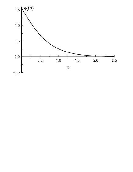
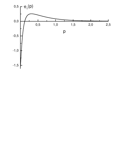
Figure 2: The ground-state (the left plot) and the first replica (the right plot) solutions of the mass-gap equation (13) after the redefinition of the chiral angle sign for odd replicas. The current quark mass is $m=0.01K_{0}$. The momentum $p$ is given in the units of $K_{0}$.

If now a small quark mass is introduced, then the vacuum energy acquires a contribution of the chirally non-invariant term proportional to the quark mass $m$ and, as a result, the whole picture gets tilted — the state with the negative sign of the chiral condensate being energetically preferable as compared to the state with the positive condensate. These two states differ by their $\theta$ coordinate — one of them corresponds to $\theta=0$, whereas the other one has $\theta=\pi$. The choice of the chiral angle adopted before, with $\varphi_{p}(0)=\frac{\pi}{2}$, selects the vacuum $\theta=0$ as the true vacuum of the theory $|0\rangle$. This is indeed the case for the ground BCS vacuum, as well as for all even replicas, with $\Sigma<0$. The pion, which is not tachyon in these vacua, is responsible for the vacuum energy increase during the rotation in the angle $\theta$ from $|0\rangle$ to $|\pi\rangle$. For odd replicas, the chiral condensate changes the sign, so that the state with $\theta=\pi$ must acquire a lower energy than the one with $\theta=0$. As a result, in odd replicas, the pion becomes the tachyon responsible for the energy decrease during the same rotation form $|0\rangle$ to $|\pi\rangle$, the latter representing now the true vacuum. Therefore, for odd replicas, we set $\varphi_{p}(0)=-\frac{\pi}{2}$ instead of $\frac{\pi}{2}$. This choice will ensure that the chiral angle, when the momentum $p$ goes to infinity, will approach zero from above. Then the chiral condensate (74) changes the sign, and so does the pion mass squared — the pion mass becomes real. As discussed before, the definition of the chiral angle admits such a change and, as a result, we arrive at two different classes of solutions to the mass-gap equation: even solutions, which start from $\frac{\pi}{2}$ at $p=0$ and approach the free limit at large $p$’s from above, and odd solutions which also approach their large-$p$ asymptote from above but, at $p=0$, start from $-\frac{\pi}{2}$. This solves the problem of the tachyon for odd replicas, making the latter normal vacuum states with the possibility of building the spectrum of hadrons above them.

As an example, we give in Fig. 2, the profiles of the ground-state and the first replica solutions to the mass-gap equation (13) for the oscillator-type potential (the case of the generalised power-like confining potential (3) is studied in detail in replica4 ). As discussed before, the sign of the chiral angle for the first replica vacuum is reversed.

In Fig. 3, we represent the solutions of the bound-state problem for the pion with the harmonic oscillator confining potential, Eq. (51), for the two lowest solutions to the mass-gap equation (13) depicted in Fig. 2 — for the ground BCS vacuum (the left plot in Fig. 3) and for the first replica with the reversed sign of the chiral angle (the right plot in Fig. 3). It is clearly seen from Fig. 3 that the pionic wave functions are indeed very close to $\pm\sin\varphi_{p}$ (see Fig. 2) with the corrections given by the formula (54). Notice that, after the change $\varphi_{p}\to-\varphi_{p}$ performed for odd replicas, the “$+$” and the “$-$” components of the mesonic wave function substitute each other, so that one needs either to redefine the whole set of the operator transformations used to diagonalise the Hamiltonian of the theory in the mesonic sector or, which is more economical, simply to rename $\varphi^{+}$ to $\varphi^{-}$ and vice versa.

         

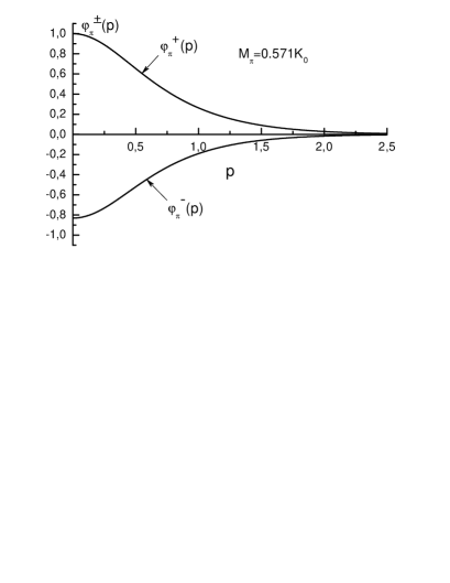
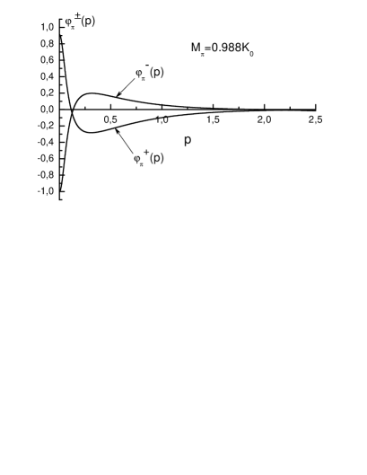
Figure 3: Solutions of the bound-state problem for the pion, Eq. (51), in the BCS vacuum (the left plot) and in the first replica with the reversed sign of the chiral angle (the right plot). The overall normalisation factor is omitted, the largest component being fixed equal to unity at $p=0$. The current quark mass is $m=0.01K_{0}$. The momentum $p$ is given in the units of $K_{0}$.

III.3 Hadronic spectrum in the replica vacua

It is concluded, in the second section, that any NJL-type Hamiltonian model with an arbitrary confining quark kernel is completely defined at BCS level, as soon as the chiral angle is built. If the large-$N_{C}$ limit is assumed, then all approximations become controllable and the Hamiltonian of the theory admits complete diagonalisation in terms of the compound mesonic operators. We found that the appropriate basis for such a diagonalisation was provided by the set $\{n,\;J^{PC}\}$ and each mesonic state was described by a pair of wave functions $\varphi^{\pm}$. In this section, following the papers replica1 ; replica2 ; replica4 , we gave evidence of existence of excited solutions to the mass-gap equation — the vacuum replicas. Now we address the question concerning the spectrum of hadrons in the replica vacua.

As argued in the previous subsection, the pion is massless in the chiral limit for any replica vacuum and, with the properly defined chiral angle, it acquires a small real mass beyond the chiral limit. As far as highly excited mesonic states are concerned, the chiral symmetry is restored in this part of the spectrum and the hadrons’ properties become insensitive to the details of the vacuum in which they are created since, for high excitations, the negative-energy components $\varphi^{-}_{n\nu}(p)$ of the wave functions are negligible and the Bethe–Salpeter bound-state equation (69) amounts to a quantum-mechanical Schrödinger equation,

$$[2E_{p}+V(r)]\varphi^{+}_{n\nu}(p)=M_{n\nu}\varphi^{+}_{n\nu}(p),\quad E_{p}=\sqrt{p^{2}+m^{2}}.$$ (75)

Consequently, no cancellations between the positive- and negative-energy components take place anymore, as it happens to the chiral pion and leads to the small pion mass of $140MeV$, as opposed the value of about $400\div 500MeV$ which would follow from Eq. (75). As a result, in the vacua with “less” broken chiral symmetry (higher replicas), the masses of mesons are pushed up, with the exception of the chiral pion, whose mass, in the chiral limit, is kept equal to zero by the requirement of the chiral symmetry. Beyond the chiral limit, the pion mass also increases with the index of the replica (see Fig. 3 and compare the pion mass of $0.57K_{0}$, in the BCS vacuum, with the value of $0.988K_{0}$, for the first replica).

Therefore, we conclude that each mesonic state can be characterised by an extra “quantum number” — the index of the vacuum replica in which it was created. Then the full diagonalised Hamiltonian of the theory takes the form:

$$\hat{\cal H}=\sum_{n,\nu,{\cal N}}M_{n\nu{\cal N}}m^{\dagger}_{n\nu{\cal N}}m_{n\nu{\cal N}}+O\left(\frac{1}{\sqrt{N_{C}}}\right),$$ (76)

${\cal N}$ being the replica label, which is the generalisation of Eq. (68) for the multi-vacuum case.

IV Conclusions

In this paper, we have shown how the generalised NJL-type Hamiltonian model with a nonlocal confining quark kernel can be fully diagonalised in the sector of physically observable hadronic states. We extend this result to include the multiple vacuum states recently found to exist in models of such a type and which are very likely to exist in real QCD. The main result of the paper is the fully diagonalised Hamiltonian (76). Similarly to the case of a path integral with a multi-minimum function in the exponent, the Hamiltonian (76) sums the contributions of all minima, with the corresponding weight — the masses of mesons in the given vacuum — being minimal for the lowest vacuum state and increasing for higher vacua, thus suppressing the contribution of the corresponding replicas to the full partition function of the theory. We study the form of the chiral angle profiles defining the excited vacua and find that for an even (odd) replica to decay to a lower even (odd) one it is sufficient to change the chiral angle in the finite region in momentum $p$, since both asymptotes for both replicas of the same parity coincide: $\varphi_{p}(p=0)=\frac{\pi}{2}\;\left(-\frac{\pi}{2}\right)$, $\varphi_{p}(p\to\infty)=0$. On the contrary, for the decay of an odd replica to an even one, or vice versa, the chiral angle has to be changed dramatically in the infrared region, since the low-momentum behaviour of even and odd replicas is quite different.

In the paper replica2 a quantum field theory perturbative method was developed. It used the replica-quark-antiquark vertex parameterised by a small difference between the chiral angles of the ground-state vacuum and the replica to evaluate the quark self-energy shift due to the replica presence. This method can be easily extended to the case of an infinite number of replicas, but notice that the sets of even and odd states have to be considered separately. As discussed above, only transformations of the chiral angle between states with the same parity are small and can be considered perturbatively. We conclude, therefore, that two sets of perturbative approaches to replicas should be built — for even and for odd replicas, independently. On the contrary, a transition between states with opposite parities, for example, the decay of the first replica to the ground BCS vacuum, involves the global transformation of the chiral angle generated by the pseudoscalar pionic operator $\hat{Q}_{5}$ and results in a burst of pions with a huge energy release. The same transition in the opposite direction — excitation of the replica — requires an external global source which is not inherent to the model. Building of such a source is an important problem in the theory of replicas and it will be the subject of future publications.

Appendix A The pion Bethe-Salpeter equation

In this appendix we derive the Bethe-Salpeter equation for the pion for the generic form of the potential and for the Lorentz structure of the confinement being $\gamma_{0}\times\gamma_{0}$. We generalise the method suggested in the paper BG for two-dimensional QCD. We start from Eq. (41) for the mesonic Salpeter amplitude and define a matrix mesonic wave function,

$$\Psi(\vec{p};M_{\pi})=\int\frac{dp_{0}}{2\pi}S(\vec{p},p_{0}+M_{\pi}/2)\chi(\vec{p};M_{\pi})S(\vec{p},p_{0}-M_{\pi}/2).$$ (77)

We also present the Dirac projectors (37) in the form:

$$\Lambda^{\pm}(\vec{p})=T_{p}P_{\pm}T_{p}^{\dagger},\quad P_{\pm}=\frac{1\pm\gamma_{0}}{2},\quad T_{p}=\exp{\left[-\frac{1}{2}(\vec{\gamma}\hat{\vec{p}})\left(\frac{\pi}{2}-\varphi_{p}\right)\right]},$$ (78)

and introduce a modified wave function $\tilde{\Psi}(\vec{p};M_{\pi})=T^{\dagger}_{p}\Psi(\vec{p};M_{\pi})T^{\dagger}_{p}$. Equation for this new matrix wave function following from Eq. (41), with $\Gamma=\gamma_{0}$, reads:

$$\tilde{\Psi}(\vec{p};M_{\pi})=-\int\frac{d^{3}q}{(2\pi)^{3}}V(\vec{p}-\vec{q})\left[P_{+}\frac{T_{p}^{\dagger}T_{q}\tilde{\Psi}(\vec{q};M_{\pi})T_{q}T_{p}^{\dagger}}{2E_{p}-M_{\pi}}P_{-}+P_{-}\frac{T_{p}^{\dagger}T_{q}\tilde{\Psi}(\vec{q};M_{\pi})T_{q}T_{p}^{\dagger}}{2E_{p}+M_{\pi}}P_{+}\right].$$ (79)

It is clear that a solution of Eq. (79) has the form,

$$\tilde{\Psi}(\vec{p};M_{\pi})=P_{+}AP_{-}+P_{-}BP_{+},$$ (80)

and, due to the obvious orthogonality property of the projectors $P_{\pm}$, $P_{+}P_{-}=P_{-}P_{+}=0$, only matrices anti-commuting with the matrix $\gamma_{0}$ contribute to $A$ and $B$. The set of such matrices is $\{\gamma_{5},\gamma_{0}\gamma_{5},\vec{\gamma},\gamma_{0}\vec{\gamma}\}$ which can be reduced even more, up to $\{\gamma_{5},\vec{\gamma}\}$, since the matrix $\gamma_{0}$ can be always absorbed into projectors $P_{\pm}$. For the case of the chiral pion only $\gamma_{5}$ contributes and one has:

$$A_{\pi}=\gamma_{5}\varphi^{+}_{\pi}(p),\quad B_{\pi}=-\gamma_{5}\varphi_{\pi}^{-}(p),$$ (81)

where the signs and the coefficients are chosen such that to comply with the definitions (29) and (49). It is an easy task now to extract the amplitudes $T_{\pi}^{\pm\pm}$ (see Eq. (34)) from Eq. (79) using the explicit form of $\tilde{\Psi}_{\pi}(\vec{p};M_{\pi})$ and the operator $T_{p}$. They read:

$$\begin{array}[]{lcr}T_{\pi}^{++}(p,q)=T_{\pi}^{-+}(p,q)&=&-\displaystyle\int d\Omega_{q}V(\vec{p}-\vec{q})\left[\cos^{2}\frac{\varphi_{p}-\varphi_{q}}{2}-\frac{1-(\hat{\vec{p}}\hat{\vec{q}})}{2}\cos\varphi_{p}\cos\varphi_{q}\right],\\[14.22636pt] T_{\pi}^{+-}(p,q)=T_{\pi}^{--}(p,q)&=&\displaystyle\int d\Omega_{q}V(\vec{p}-\vec{q})\left[\sin^{2}\frac{\varphi_{p}-\varphi_{q}}{2}+\frac{1-(\hat{\vec{p}}\hat{\vec{q}})}{2}\cos\varphi_{p}\cos\varphi_{q}\right].\end{array}$$ (82)

For the harmonic oscillator potential, and with the amplitudes (82), Eq. (34) reproduces Eq. (51).

In the chiral limit, $\varphi_{\pi}^{+}(p)=-\varphi_{\pi}^{-}(p)=\varphi_{\pi}(p)$, so that the bound-state equation (34) reduces to a single equation,

$$2E_{p}\varphi_{\pi}(p)=\int\frac{q^{2}dq}{(2\pi)^{3}}[T_{\pi}^{++}(p,q)-T_{\pi}^{+-}(p,q)]\varphi_{\pi}(q)=-\int\frac{d^{3}q}{(2\pi)^{3}}V(\vec{p}-\vec{q})\varphi_{\pi}(q),$$ (83)

or, in the coordinate space, one arrives at the Schrödinger-like equation,

$$[2E_{p}+V(r)]\varphi_{\pi}=0.$$ (84)

It is also instructive to derive the bound-state equation for the pionic matrix wave function $\Psi(\vec{p};M_{\pi})$. It follows directly from the representation (79) after a simple algebra (see 2d for the detailed discussion of the matrix wave function formalism in two-dimensional QCD),

$$M_{\pi}\Psi(\vec{p};M_{\pi})=[(\vec{\alpha}\vec{p})+\gamma_{0}m]\Psi(\vec{p};M_{\pi})+\Psi(\vec{p};M_{\pi})[(\vec{\alpha}\vec{p})-\gamma_{0}m]\hskip 142.26378pt$$

$$+\int\frac{d^{3}q}{(2\pi)^{3}}V(\vec{p}-\vec{q})\left\{\Lambda^{+}(\vec{q})\Psi(\vec{p};M_{\pi})\Lambda^{-}(-\vec{q})-\Lambda^{+}(\vec{p})\Psi(\vec{q};M_{\pi})\Lambda^{-}(-\vec{p})\right.$$ (85)

$$\hskip 142.26378pt\left.-\Lambda^{-}(\vec{q})\Psi(\vec{p};M_{\pi})\Lambda^{+}(-\vec{q})+\Lambda^{-}(\vec{p})\Psi(\vec{q};M_{\pi})\Lambda^{+}(-\vec{p})\right\}.$$

The explicit form of $\Psi(\vec{p};M_{\pi})$ through the components $\varphi_{\pi}^{\pm}$ and the chiral angle can be found easily from Eqs. (80), (81),

$$\Psi(\vec{p};M_{\pi})=T_{p}\left[P_{+}\gamma_{5}\varphi_{\pi}^{+}-P_{-}\gamma_{5}\varphi_{\pi}^{-}\right]T_{p}=\gamma_{5}G_{\pi}+\gamma_{0}\gamma_{5}T_{p}^{2}F_{\pi},$$ (86)

where $G_{\pi}=\frac{1}{2}(\varphi_{\pi}^{+}-\varphi_{\pi}^{-})$, $F_{\pi}=\frac{1}{2}(\varphi_{\pi}^{+}+\varphi_{\pi}^{-})$.

Let us multiply the matrix bound-state equation (85) by $\gamma_{0}\gamma_{5}$, integrate its both parts over $d^{3}p$, and, finally, take the trace. The resulting equation reads:

$$M_{\pi}\int\frac{d^{3}p}{(2\pi)^{3}}F_{\pi}\sin\varphi_{p}=2m\int\frac{d^{3}p}{(2\pi)^{3}}G_{\pi}.$$ (87)

It is easy to recognise the Gell-Mann–Oakes–Renner relation (18) in Eq. (87). Indeed, using the explicit form of the pionic wave function beyond the chiral limit, Eq. (54), one can see that $G_{\pi}=(\tilde{\cal N}_{\pi}/\sqrt{M_{\pi}})\sin\varphi_{p}$ and $F_{\pi}=(\tilde{\cal N}_{\pi}\sqrt{M_{\pi}})\Delta_{p}$ which, after substitution to Eq. (87), give the sought relation,

$$M_{\pi}^{2}\left[\frac{N_{C}}{\pi^{2}}\int_{0}^{\infty}dp\;p^{2}\Delta_{p}\sin\varphi_{p}\right]=-2m\langle\bar{q}q\rangle,$$ (88)

where the definition of the chiral condensate (74) was used.