UCT-TP-262/04

September 2004

Electromagnetic proton form factors in large $N_{c}$ QCD
C. A. Dominguez, T. Thapedi
Institute of Theoretical Physics and Astrophysics

University of Cape Town, Rondebosch 7700, South Africa

Abstract

The electromagnetic form factors of the proton are obtained using a particular realization of QCD in the large $N_{c}$ limit ($\mbox{QCD}_{\infty}$), which sums up the infinite number of zero-width resonances to yield an Euler’s Beta function (Dual-$\mbox{QCD}_{\infty}$). The form factors $F_{1}(q^{2})$ and $F_{2}(q^{2})$, as well as $G_{M}(q^{2})$ agree very well with reanalyzed space-like data in the whole range of momentum transfer. In addition, the predicted ratio $\mu_{p}G_{E}/G_{M}$ is in good agreement with recent polarization transfer measurements at Jefferson Lab.

Quantum Chromodynamics (QCD) in the limit of large number of colours ($\mbox{QCD}_{\infty}$) [1] is known to predict a hadronic spectrum consisting of an infinite number of zero-width resonances[2]. However, since real QCD has never been solved exactly and analytically, the hadronic parameters (masses, couplings, etc.) remain unpredicted. A few models of this spectrum have been proposed for heavy quark Green’s functions [3]-[4], as well as for light quark systems [5]. The infinite number of zero-width resonances of $\mbox{QCD}_{\infty}$ is reminiscent of Veneziano’s dual-resonance model [6], the precursor of string theory. In fact, inspiration from this model has led to a proposal called Dual-$\mbox{QCD}_{\infty}$ [7], a specific realization of $\mbox{QCD}_{\infty}$ where the masses and couplings in a Green’s function are chosen to yield an Euler’s Beta function of the Veneziano type. For three-point functions, the form factors exhibit asymptotic Regge-behaviour, i.e. power-behaviour, in the space-like region controlled by a single free parameter. Dual-$\mbox{QCD}_{\infty}$ has been applied quite successfully to the electromagnetic form factor of the pion in the space-like region [7]. Indeed, results are in excellent agreement with experiment, far better than e.g. naive Vector Meson (rho-) Dominance or purely perturbative QCD [8]. This is the case not only for the pion form factor itself, but also for the mean-square radius, and the observed deviation from universality (the ratio $g_{\rho\pi\pi}/f_{\rho}$) . In addition, unitarization of Dual-$\mbox{QCD}_{\infty}$ leads to a prediction of the vector two-point spectral function, in the time-like region, in reasonable agreement with data (a more refined model in the time-like region has been proposed recently in [9]). Encouraged by this success, we discuss in this note an analysis of the electromagnetic proton form factors in the framework of Dual-$\mbox{QCD}_{\infty}$.

The Dirac and Pauli form factors of the proton, $F_{1}(q^{2})$ and $F_{2}(q^{2})$, respectively, are defined as

$$<N(p_{2})|J_{\mu}^{EM}(0)|N(p_{1})>=\bar{u}_{N}(p_{2})\;[F_{1}(q^{2})\gamma_{\mu}+\frac{i\kappa}{2M_{p}}F_{2}(q^{2})\sigma_{\mu\nu}q^{\nu}]\;u_{N}(p_{1})\;,$$ (1)

where $q^{2}=(p_{2}-p_{1})^{2}$, while $\kappa\equiv\mu_{p}-1$, and $M_{p}$ are the proton’s magnetic moment and mass, respectively, and $F_{1,2}(q^{2})$ are normalized as $F_{1}(0)=F_{2}(0)=1$. On the other hand, the Sachs’ form factors $G_{E}(q^{2})$ and $G_{M}(q^{2})$ are given by

$$\begin{array}[]{lcl}G_{E}(q^{2})&=&F_{1}(q^{2})-\kappa\;\tau\;F_{2}(q^{2})\\ G_{M}(q^{2})&=&F_{1}(q^{2})+\kappa\;F_{2}(q^{2})\;,\end{array}$$ (4)

where $\tau=-q^{2}/4M_{p}^{2}\equiv Q^{2}/4M_{p}^{2}$, and the normalization is then $G_{E}(0)=1$, and $G_{M}(0)=\mu_{p}$.
In the very early applications of the dual-resonance model to three point functions involving more than one form factor [10], it was not quite clear to which form factor, or linear combination of form factors, should the model apply. There is no ambiguity in Dual-$\mbox{QCD}_{\infty}$, as this is a realization of a quantum field theory. The form factors should then be those appearing in the primary hadronic spectral function, dual to the QCD field theory spectral function. In other words, the form factors with the correct pole structure satisfying dispersion relations in the complex energy plane. In the case of the nucleon, these are the Dirac and Pauli form factors which in $\mbox{QCD}_{\infty}$ become

$$F_{1,2}(s)=\sum_{n=0}^{\infty}\frac{C_{(1,2)n}}{(M_{n}^{2}-s)}\;,$$ (5)

where $s\equiv q^{2}$, and the masses of the vector-meson zero-width resonances, $M_{n}$, as well as their couplings $C_{1n}$ and $C_{2n}$, are not predicted. In Dual-$\mbox{QCD}_{\infty}$ these are chosen so that the form factors become Beta functions (ratios of gamma-functions), i.e.

$$C_{(1,2)n}=\frac{\Gamma(\beta_{1,2}-1/2)}{\alpha^{\prime}\sqrt{\pi}}\;\frac{(-1)^{n}}{\Gamma(n+1)}\;\frac{1}{\Gamma(\beta_{1,2}-1-n)}\;,$$ (6)

where $\beta_{1,2}$ are free parameters controlling the asymptotic behaviour in the space-like region ($s<0$), and $\alpha^{\prime}=1/2M_{\rho}{{}^{2}}$ is the universal string tension in the rho-meson Regge trajectory

$$\alpha_{\rho}(s)=1+\alpha^{\prime}(s-M_{\rho}^{2})\;.$$ (7)

The mass spectrum is chosen as [11]

$$M_{n}^{2}=M_{\rho}^{2}(1+2n)\;.$$ (8)

Using Eqs.(4) and (6) in Eq.(3) one obtains

$$F_{1,2}(s) = \frac{\Gamma(\beta_{1,2}-1/2)}{\sqrt{\pi}}\;\sum_{n=0}^{\infty}\;\frac{(-1)^{n}}{\Gamma(n+1)}\;\frac{1}{\Gamma(\beta_{1,2}-1-n)}\;\frac{1}{[n+1-\alpha_{\rho}(s)]}$$ (9)

$$= \frac{1}{\sqrt{\pi}}\;\frac{\Gamma(\beta_{1,2}-1/2)}{\Gamma(\beta_{1,2}-1)}\;\;B(\beta_{1,2}-1,\;1/2-\alpha^{\prime}s)\;,$$

where B(x,y) is Euler’s Beta function. In the time-like region ($s>0$) the poles of the Beta function correspond to an infinite set of zero-width resonances with equally spaced squared masses given by Eq.(5). In fact, from Eq.(7) it follows

$$Im\;F_{1,2}(s)=\frac{\Gamma(\beta_{1,2}-1/2)}{\alpha^{\prime}\sqrt{\pi}}\;\sum_{n=0}^{\infty}\;\frac{(-1)^{n}}{\Gamma(n+1)}\;\frac{1}{\Gamma(\beta_{1,2}-1-n)}\;\pi\;\delta(M_{n}^{2}-s)\;.$$ (10)

Asymptotically, the form factors in the space-like region exhibit Regge-behaviour, viz.

$$\lim_{s\rightarrow-\infty}F_{1,2}(s)=(-\alpha^{\prime}\;s)^{(1-\beta_{1,2})}\;,$$ (11)

The free parameters $\beta_{1,2}$ can be fixed from fits to the data in the space-like region. Notice that the values $\beta_{1,2}=2$ reduce the form factors to single rho-meson dominance (naive Vector Meson Dominance). The mass formula Eq.(6) predicts e.g. for the first three radial excitations: $M_{\rho^{\prime}}\simeq 1340$ MeV, $M_{\rho^{\prime\prime}}\simeq 1720$ MeV, and $M_{\rho^{\prime\prime\prime}}\simeq 2034$ MeV in reasonable agreement with experiment [12] : $M_{\rho^{\prime}}=1465\pm 25$ MeV, $M_{\rho^{\prime\prime}}=1700\pm 20$ MeV, and $M_{\rho^{\prime\prime\prime}}=2149\pm 17$ MeV. Alternative (non-linear) mass formulas might be required if one were to match the asymptotic Regge behaviour to the Operator Product Expansion of current correlators at short distances [13]. However, the differences in the values of the first few masses are at the level of a few percent. Hence, the form factors would hardly be affected, since the contribution from high mass states is factorially suppressed.

Historically, the Sachs form factors were first determined from measurements of elastic electron-proton scattering cross sections (Rosenbluth technique) [14]. Direct extractions of $G_{E}(q^{2})$ and $G_{M}(q^{2})$ up to $-q^{2}\equiv Q^{2}\simeq 7\;\mbox{GeV}^{2}$ indicated the empirical approximate scaling relation: $\mu_{p}G_{E}(q^{2})/G_{M}(q^{2})\simeq 1$. At higher values of $Q^{2}$, the contribution of $G_{E}(q^{2})$ to the cross section is kinematically suppressed. On the other hand, recent electron-proton polarization transfer measurements at Jefferson Lab (JLab) [15] up to $Q^{2}\simeq 6\;\mbox{GeV}^{2}$ show a considerable deviation from this scaling behaviour, except possibly at very small $Q^{2}$ [16]. After some debate about the source of the discrepancy between cross-section (Rosenbluth) and polarization transfer extractions of the form factors [17], it appears that the culprit is the two-photon exchange correction [18]. We assume this to be the case, and adopt the experimental data on the Sachs form factors as corrected in [19]. These corrections are made in order to bring the Rosenbluth data into agreement with the polarization transfer data on the ratio $\mu_{p}G_{E}(q^{2})/G_{M}(q^{2})$. We then use Eq.(2) to obtain data points for $F_{1}(q^{2})$ and $F_{2}(q^{2})$. After fitting this data base with Eq.(7) we find $\beta_{1}=3.03$, and $\beta_{2}=4.20$. Figures 1, and 2 show the results of the fits for $F_{1}(q^{2})$, and $F_{2}(q^{2})$, corresponding to these values of $\beta_{1,2}$, together with the corrected data points of [19]. In Fig. 3 we show $G_{M}(q^{2})$, as obtained from Eq.(2) using the fitted $F_{1,2}(q^{2})$, together with the same data base. As can be appreciated, the agreement between Eq.(7) and the data is very good. Having fitted a data base corrected to account for the polarization transfer data on the ratio $\mu_{p}G_{E}(q^{2})/G_{M}(q^{2})$, we would expect our theoretical form factors to lead to a ratio in agreement with experiment. While this is the case, it turns out that this ratio is very sensitive to the pair of values $\beta_{1}-\beta_{2}$, with a strong correlation between them. In Fig. 4 we show the theoretical prediction of the ratio $\mu_{p}G_{E}(q^{2})/G_{M}(q^{2})$ corresponding to $\beta_{1}=3.0$ and $\beta_{2}=4.2$, together with the JLab data [15]. Small variations of these parameters lead to correlated pairs resulting in equally good fits, e.g. the pair $\beta_{1}=2.95$ and $\beta_{2}=4.13$ leads to an almost identical theoretical prediction. Exploring the $\beta_{1}$-$\beta_{2}$ parameter space, and performing a combined fit to $F_{1}(q^{2})$, $F_{2}(q^{2})$, and the ratio $\mu_{p}G_{E}(q^{2})/G_{M}(q^{2})$ gives

$$\begin{array}[]{lcl}\beta_{1}&=&2.95-3.03\\ \beta_{2}&=&4.13-4.20\;.\end{array}$$ (14)

The mean-squared electromagnetic radii that follow from Eq.(7) are given by

$$<r^{2}_{1,2}>=6\;\alpha^{\prime}\;[\psi(\beta_{1,2}-1/2)-\psi(1/2)]\;,$$ (15)

where $\psi(x)$ is the digamma function. Using the results from Eq.(10) in Eq. (11) gives $<r^{2}_{1}>^{1/2}=0.72\;fm$, and $<r^{2}_{2}>^{1/2}=0.78\;fm$. From Eq.(2), these radii lead to the Sachs radii $<r^{2}_{E}>^{1/2}=0.81\;fm$, and $<r^{2}_{M}>^{1/2}=0.76\;fm$. These values are in reasonable agreement with various other results in the literature [20], especially taking into account that the free parameters $\beta_{1,2}$ have been fixed from the large-$Q^{2}$ data, while the form factors decrease by 3-4 orders of magnitude in the range $0\leq Q^{2}\mbox{\raisebox{-2.15277pt}{$\;\sim$} \raisebox{3.44444pt}{$\!\!\!\!\!\!\!<$}}\;30\;\mbox{GeV}^{2}$. It should also be kept in mind that the strong deviation from unity of the ratio $\mu_{p}G_{E}(q^{2})/G_{M}(q^{2})$ might affect existing extractions of the Sachs radii from data.

In summary, the nucleon form factors $F_{1}(q^{2})$, and $F_{2}(q^{2})$ obtained in the framework of Dual-$\mbox{QCD}_{\infty}$ reproduce very nicely the experimental data in the space-like region, as corrected in [19], in the wide range $0\leq Q^{2}\mbox{\raisebox{-2.15277pt}{$\;\sim$} \raisebox{3.44444pt}{$\!\!\!\!\!\!\!<$}}\;30\;\mbox{GeV}^{2}$. The Sachs magnetic form factor, $G_{M}(q^{2})$, as well as the non-trivial ratio $\mu_{p}G_{E}(q^{2})/G_{M}(q^{2})$ can also be accounted for in this framework. These results provide strong support for Dual-$\mbox{QCD}_{\infty}$ as a viable realization of QCD in the large $N_{c}$ limit.

Acknowledgements
One of us (CAD) wishes to thank F. Maas for a very helpful discussion on the experimental data.

Figure Captions

Figure 1. Dual-$QCD_{\infty}$ form factor $F_{1}(Q^{2})$, Eq.(7), for the fitted parameter $\beta_{1}=3.03$, together with the experimental data as corrected in [19].

Figure 2. Dual-$QCD_{\infty}$ form factor $F_{2}(Q^{2})$, Eq.(7), for the fitted parameter $\beta_{2}=4.20$, together with the experimental data as corrected in [19].

Figure 3. Dual-$QCD_{\infty}$ form factor $G_{M}(Q^{2})$, Eq.(2), for the fitted parameters $\beta_{1}=3.03$, and $\beta_{2}=4.20$, together with the experimental data as corrected in [19].

Figure 4. Dual-$QCD_{\infty}$ ratio $\mu_{p}G_{E}(Q^{2})/G_{M}(Q^{2})$ for the fitted parameters $\beta_{1}=3.00$, and $\beta_{2}=4.20$, together with the experimental data [15].

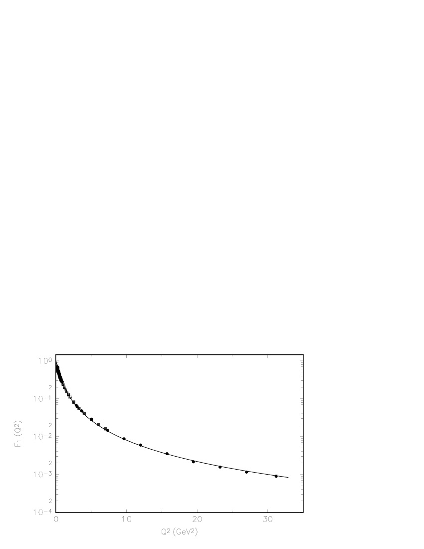
Figure 1:

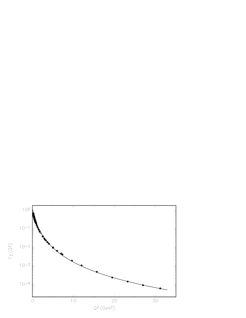
Figure 2:

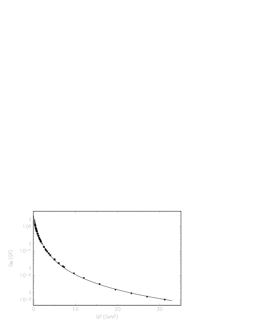
Figure 3:

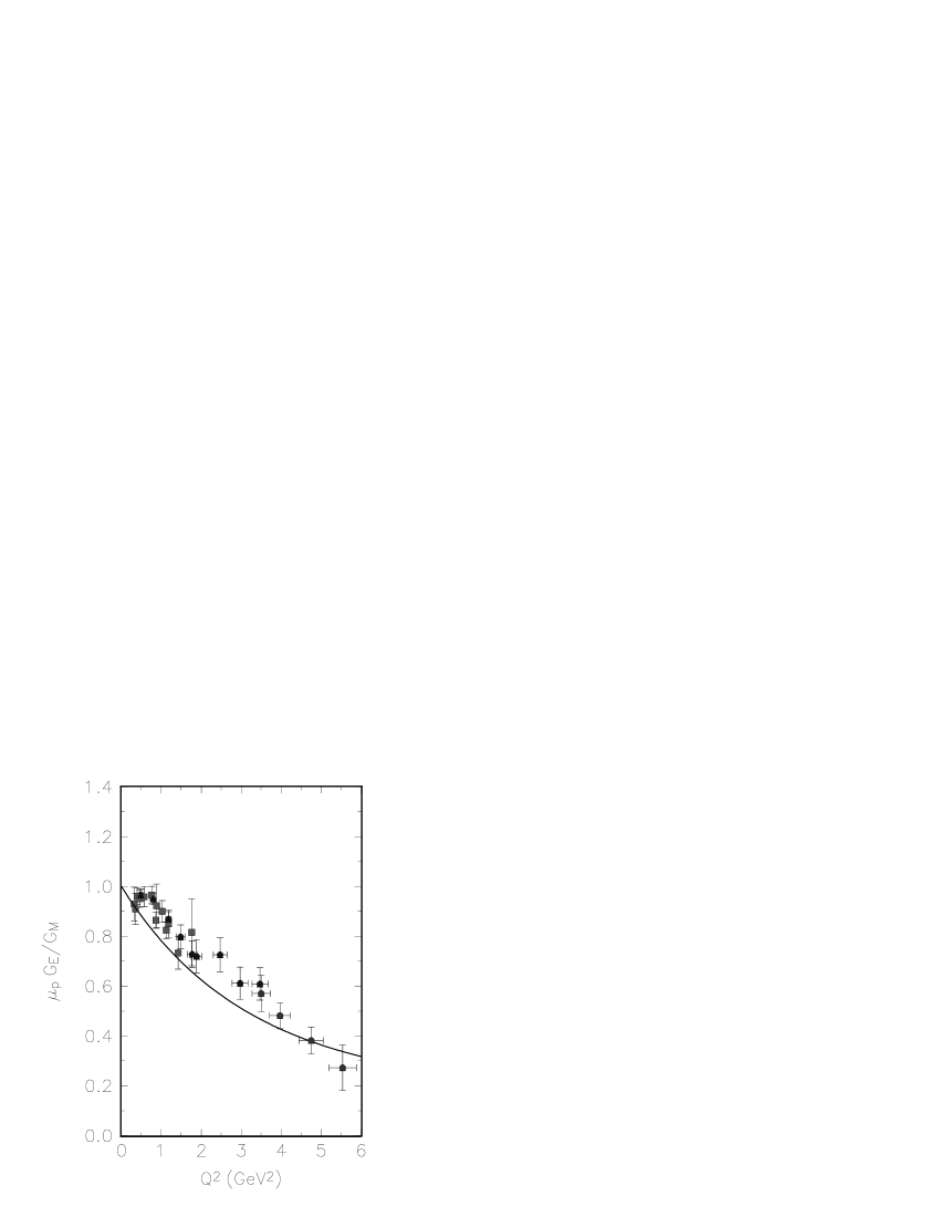
Figure 4:

References

- [1] G. ’t Hooft, Nucl. Phys. B 72 (1974) 461.
- [2] E. Witten, Nucl. Phys. B 79 (1979) 57.
- [3] B. Chibisov et al. Int. J. Mod. Phys. A 12 (1997) 2075; B. Blok, M. Shifman and Da-Xin Zhang, Phys. Rev. D 57 (1998) 2691.
- [4] P. Colangelo, C.A. Dominguez and G. Nardulli, Phys. Lett. B 409 (1997) 417.
- [5] S. Peris, B. Phily, E. de Rafael, Phys. Rev. Lett. 86 (2001) 14, and references therein.
- [6] P.H. Frampton, Dual Resonance Models, Benjamin (1974).
- [7] C.A. Dominguez, Phys. Lett. B 512 (2001) 331.
- [8] C.A. Dominguez, Phys. Rev. D 25 (1982) 3084.
- [9] C. Bruch, A. Khodjamirian, J.H. Kühn, hep-ph/0409080 (2004).
- [10] P.H. Frampton, Phys. Rev. D 1 (1970) 3141; R. Iengo, E. Remiddi, Nuovo Cimento Lett. 18 (1969) 922; C.A. Dominguez, O. Zandron, Nucl.Phys. B 33 (1971) 303; C.A. Dominguez, Phys. Rev. D 8 (1973) 980.
- [11] This mass formula was first proposed in a different context by A. Bramon, E. Etim, M. Greco, Phys. Lett. 41 B (1972) 609; M. Greco, Nucl. Phys. B 63 (1973) 398.
- [12] Particle Data Group, K. Hagiwara et al., Phys. Rev. D 66 (2002) 010001.
- [13] S.S. Afonin, A.A. Andrianov, V.A. Andrianov, D. Espriu, J. High Energy Phys. 04 (2004) 039.
- [14] T. Janssens et al. Phys. Rev. D 142 (1966) 922; J. Litt et al., Phys. Lett. 31 B (1970) 40; Ch. Berger et al., Phys. Lett. 35 B (1971) 87; W. Bartel et al., Nucl. Phys. B 58 (1973) 429; A.F. Sill et al., Phys. Rev. D 48 (1993) 29; R.C. Walker et al., Phys. Rev. D 49 (1994) 5671; L. Andivahis et al., Phys. Rev. D 50 (1994) 5491; M.E. Christy et al., Phys. Rev. C 70 (1994) 015206.
- [15] M.K. Jones et al., Phys. Rev. Lett. 84 (2000) 1398; O. Gayou et al., Phys. Rev. C 64 (2001) 038202; O. Gayou et al., Phys. Rev. Lett. 88 (2002) 092301.
- [16] B.D. Milbrath et al., Phys. Rev. Lett. 80 (1998) 452; ibid. 82 (1999) 2221 (E).
- [17] J. Arrington, Phys. Rev. C 68 (2003) 034325; ibid. C 69 (2004) 022201.
- [18] P. Guichon, M. Vanderhaeghen, Phys. Rev. Lett. 91 (2003) 142303; P.G. Blunden, W. Melnitchouk, J.A. Tjon, Phys. Rev. Lett. 91 (2003) 142304; J. Arrington, Phys. Rev. C 69 (2004) 022201; ibid. Phys. Rev. C 69 (2004) 032201; Y.-C. Chen et al. hep-ph/0403058 (2004).
- [19] E.J. Brash, A. Kozlov, Sh. Li, G.M. Huber, Phys. Rev. C 65 (2002) 051001.
- [20] P. Mergell, Ulf-G. Meissner, D. Dreschel, Nucl. Phys. A 596 (1996) 367, and references therein.