Searching for realistic 4d string models with a Pati-Salam symmetry
– Orbifold grand unified theories from heterotic string compactification on a $\mathbb{Z}_{6}$ orbifold

Abstract

Motivated by orbifold grand unified theories, we construct a class of three-family Pati-Salam models in a ${\mathbb{Z}}_{6}$ abelian symmetric orbifold with two discrete Wilson lines. These models have marked differences from previously-constructed three-family models in prime-order orbifolds. In the limit where one of the six compactified dimensions (which lies in a ${\mathbb{Z}}_{2}$ sub-orbifold) is large compared to the string length scale, our models reproduce the supersymmetry and gauge symmetry breaking pattern of 5d orbifold grand unified theories on an ${\rm S^{1}}/{\mathbb{Z}}_{2}$ orbicircle. We find a horizontal $2+1$ splitting in the chiral matter spectra – 2 families of matter are localized on the ${\mathbb{Z}}_{2}$ orbifold fixed points, and 1 family propagates in the 5d bulk – and identify them as the first-two and third families. Remarkably, the first two families enjoy a non-abelian dihedral ${\rm{D}_{4}}$ family symmetry, due to the geometric setup of the compactified space. In all our models there are always some color triplets, i.e. $({\bf 6,1,1})$ representations of the Pati-Salam group, survive orbifold projections. They could be utilized to spontaneously break the Pati-Salam symmetry to that of the Standard Model. One model, with a 5d E₆ symmetry, may give rise to interesting low energy phenomenology. We study gauge coupling unification, allowed Yukawa couplings and some of their phenomenological consequences. The ${\rm{E}_{6}}$ model has a renormalizable Yukawa coupling only for the third family. It predicts a gauge-Yukawa unification relation at the 5d compactification scale, and is capable of generating reasonable quark/lepton masses and mixings. Potential problems are also addressed, they may point to the direction for refining our models.

I Introduction and motivation

The Standard Model (SM) has been a cornerstone of modern-day particle physics. Although during the past three decades it has passed all experimental tests, nevertheless there are many open questions remaining to be answered. We have yet to understand — (i) the mechanism of electro-weak symmetry breaking, and find the Higgs boson which might be responsible for this breaking; (ii) the quantized fermion charges (why the up and down quarks have charges $2/3$ and $-1/3$ respectively) and the weak mixing angle (why it is 0.23); (iii) the 3 replicas of quarks and leptons, the observed fermion mass hierarchy, and the Cabibbo-Kobayashi-Maskawa (CKM) mixing matrix and its leptonic cousin. We ought to understand these problems from more fundamental principles, rather than simply take various charges, masses, mixing angles and CP phases as input parameters as in the SM. Addressing these questions may eventually lead us to a more fundamental theory such as string theory at high energy scales.

String theory GSW is a leading candidate for a consistent theory of quantum gravity. It has a rich structure and many believe it can easily accommodate the SM as a subset. Moreover there have been many attempts in the past to construct supersymmetric generalizations of the SM (which will be loosely referred to as the minimal supersymmetric standard model, or the MSSM) or grand unified theories (GUTs) from the heterotic string het ; CY ; Dixon ; Schellekens ; BL and superstrings os . Partially successful results have been obtained. For example, many string theoretical models can explain the existence of three chiral families at low energy scales greene ; IMNQ ; IMNQ2 ; FIQS ; ff ; sgut ; ALR ; os , and in principle can also provide a natural framework for understanding the fermion masses and mixings fm . In this paper, we construct a new class of three-family models in the heterotic string theory.

Before presenting our models, it is important to note some caveats common to all known string models. They are due to two main difficulties facing the string theoretical model constructions. The first difficulty concerns the compactification of the string itself, i.e. the mechanism by which the desirable string vacuum is selected. The vacua of string theory compactifications are parameterized by many scalar fields with flat potentials. These fields are the modulus fields. They characterize the sizes and shapes of the compactified spaces and the strengths of the string interactions; none of them can be fixed in perturbation theory ds . The modulus problem and the related issue of supersymmetry breaking will not be dealt with in this article, instead we will simply assume that the moduli are fixed by some unknown mechanism at the string scale.

The second difficulty concerns our ignorance of the physics between the electro-weak and unification scales. Except for some indication that the SM gauge couplings may unify at about $10^{16}$ GeV in certain supersymmetric extensions of the SM with minimal matter content unif , we can hardly have any confidence in extrapolating the low energy data by some $14$ to $16$ orders of magnitude to the unification scale and infer what the gauge symmetries, matter spectra and physical parameters are at that scale. Hence, we are far from having a clear-cut field theoretical model at the unification scale to which a string-derived model is supposed to match. Any string construction must combine both bottom-up and top-down analyses.

The new class of string models in this paper are mainly motivated by the recent discussions on orbifold GUT models kawamura ; OGUT . These GUT models utilize properties of higher-dimensional field theories, and have some advantages over conventional 4d GUTs. For example, GUT symmetry breaking can be accomplished by an orbifold parity, instead of by a complicated Higgs sector. The doublet-triplet splitting problem, which plagues conventional GUTs, can also be solved by assigning appropriate orbifold parities to the doublet and triplet Higgs bosons. Note, however, that like all field theoretical models in higher dimensions, these GUT models are not renormalizable quantum field theories. They can only make sense as low-energy effective theories of some more fundamental theory with better ultra-violet (UV) behavior. Our string models provide exactly such kind of UV completions, in the sense that they reproduce many interesting features of the orbifold GUTs in certain low energy limits. (Connections between orbifold GUTs and an ${\rm{SO}_{10}}$ string model have already been established in ref. KRZ0 . The present paper contains more detailed discussions on these connections. See also the recent paper Forste:2004ie .)

To make the connections between string and field theoretical models more concrete, we consider some examples, in particular, the 5d ${\rm{SO}_{10}}$ model of ref. OGUT and a generalization with bulk gauge group E₆. In these models, the extra dimension is taken to be an orbicircle ${\rm S^{1}}/{\mathbb{Z}}_{2}$ and the 4d effective theory has a Pati-Salam (PS) symmetry, $\rm SU_{4C}\times SU_{2L}\times SU_{2R}$ PS . The technical apparatus we adopt to build string models is the simplest abelian symmetric orbifold compactification Dixon ; BL ; IMNQ ; IMNQ2 ; FIQS ; katsuki of the heterotic string het . More specifically, we consider a non-prime-order ${\mathbb{Z}}_{6}$ orbifold (or equivalently, ${\mathbb{Z}}_{2}\times{\mathbb{Z}}_{3}$) model with the orbifold twist vector ${\bf v}_{6}=\frac{1}{6}(1,2,-3)$. To achieve three chiral PS families at low energies, we also introduce several (in fact, two) discrete Wilson lines wl . It is obvious that the third compactified complex dimension has a ${\mathbb{Z}}_{2}$ symmetry in the ${\mathbb{Z}}_{6}$ model, hence it can consistently be taken to be the root lattice of the ${\rm{SO}_{4}}$ Lie algebra. The string models are effectively 5d when the length of one of the ${\rm{SO}_{4}}$ simple roots is large compared to the string scale, while all other dimensions are kept comparable to the string scale (i.e. the geometry of the compactified space is equivalent to that of the orbifold GUTs, ${\rm S^{1}}/{\mathbb{Z}}_{2}$). In this limit, the ${\mathbb{Z}}_{6}$ heterotic models are similar to the orbifold GUT models in the following respects:

• The 5d ${\mathcal{N}}=2$ supersymmetry is broken to that of ${\mathcal{N}}=1$ in 4d by the ${\mathbb{Z}}_{2}$ orbifold twist and the “bulk” gauge group is broken to two different regular subgroups at the two inequivalent fixed points by degree-2 non-trivial gauge embedding and Wilson line. The surviving gauge group in the 4d effective theory is the intersection of groups at the fixed points. It is the PS group in our models. More specifically, we find two types of models. In the first type we have an ${\rm{E}_{6}}$ symmetry in the 5d bulk which is broken to ${\rm{SO}_{10}}$ and ${\rm{SU}_{6}}\times{\rm{SU}_{2}}$ respectively. In the second type we have an ${\rm{SO}_{10}}\times{\rm{SU}_{2}}$ in the bulk, broken to PS at one of the two fixed points.

• Untwisted-sector and twisted-sector states that are not localized on the ${\mathbb{Z}}_{2}$ fixed points of the ${\rm{SO}_{4}}$ lattice can be identified with the “bulk” states of the orbifold GUT. Interpretation of the Kaluza-Klein (KK) towers of the bulk gauge and matter fields agree in the string-based and orbifold GUT models.

• Twisted-sector states that are localized on the ${\mathbb{Z}}_{2}$ fixed points of the ${\rm{SO}_{4}}$ lattice have no field theoretical counterparts, although they can correctly be identified with the “brane” states of the orbifold GUT. In the orbifold GUT models, these states are only constrained by the requirement of (chiral) anomaly cancellation.

Of course, string theoretical models are more intricate than the corresponding field theoretic orbifold GUT models. They need to satisfy more stringent consistency conditions and thus they are physically more constrained. We find it is highly non-trivial (or impossible) to implement all the features of the orbifold GUTs. For example, we cannot arbitrarily place the three families of quarks and leptons in the bulk or on either brane. Moreover, the very act of obtaining three families, along with their respective locations, is fixed by the requirement that the gauge embeddings and Wilson lines have to satisfy the modular invariance conditions Dixon ; vafa . In addition, we cannot utilize the orbifold projections to remove all the $({\bf 6},{\bf 1},{\bf 1})$ color-triplet states as in the ${\rm{SO}_{10}}$ orbifold GUTs OGUT and at the same time obtain three families. We also find many massless states carrying unconventional representations under the SM gauge group. These exotic states are commonplace in almost all known three-family models. Whether these models can give rise to satisfactory phenomenology needs more detailed knowledge of the low-energy effective actions. The present status of our analysis is contained in this paper.

The paper is organized as follows. In sect. II we briefly review 5d field theories on the orbicircle ${\rm S^{1}}/{\mathbb{Z}}_{2}$ and present two orbifold GUT models with bulk gauge groups ${\rm{SO}_{10}}$ and ${\rm{E}_{6}}$. The latter (model A1) is a novel 5d model with many nice phenomenological features. Then in sect. III we discuss the heterotic string construction of model A1. Using this model as a guide we compare the heterotic string construction with generic orbifold GUT models by restricting the compactified space to a specific type (which is referred to as the orbifold GUT limit). We show the equivalence between the matter states (in the untwisted and some twisted sectors) in string-based models and the bulk states in orbifold GUTs, as well as their KK excitations. We interpret orbifold parities (for the bulk states) in the orbifold GUTs in string theory language, and explain why the gauge embeddings and Wilson lines cannot project away all the $({\bf 6,1,1})$ color-triplet states. These states may be needed to break the PS group to that of the SM, as in the field theoretical model of sect. II.2. In sect. IV we focus on more of the phenomenological aspects of model A1. In sect. IV.1 we discuss gauge coupling unification and the determination of the compactification and string scales. In sect. IV.2 we examine the allowed Yukawa couplings (at both the renormalizable and non-renormalizable levels) and their phenomenological consequences, concentrating on the possibility of breaking the PS symmetry, mass generation for the color-triplet fields and SM fermions, and proton stability. We conclude in sect. V, listing the pros and cons of the present models. Hopefully one can learn from the problems to design better models in the future.

We have made an effort to make the paper more accessible to field theory model builders. Many of the details of string constructions are relegated to four appendices. In appendix A we review the construction of non-prime-order orbifold models with Wilson lines, highlighting its differences with the prime-order orbifold construction. In appendix B.1 we present three three-family ${\mathbb{Z}}_{6}$ models with PS gauge symmetry. The complete matter spectra are listed in appendix B.2, where we also explain the notation for the twisted-sector states. In appendix C.1 we review the string selection rules necessary for determining non-trivial Yukawa couplings in a 4d effective theory, and in appendix C.2 list some allowed couplings involving operators of interest in model A1. Finally, in appendix D we study gauge coupling unification and derive the Georgi-Quinn-Weinberg (GQW) relations GQW in the orbifold GUT limit. These relations allow us to determine various mass scales in our models.

II 5d orbifold GUT models on ${\rm S^{1}}/{\mathbb{Z}}_{2}$

Let us briefly review the geometric picture of orbifold GUT models compactified on an orbicircle ${\rm S}^{1}/{\mathbb{Z}}_{2}$. The space group of ${\rm S}^{1}/\mathbb{Z}_{2}$ is composed of two actions, a translation, ${\cal T}:\,x^{5}\rightarrow x^{5}+2\pi R$, and a space reversal, ${\cal P}:\,x^{5}\rightarrow-x^{5}$. There are two (conjugacy) classes of fixed points, $x^{5}=2n\pi R$ and $(2n+1)\pi R$, where $n\in\mathbb{Z}$.

The space group multiplication rules imply ${\cal T}{\cal P}{\cal T}={\cal P}$, so we can replace the translation by a composite $\mathbb{Z}_{2}$ action ${\cal P}^{\prime}={\cal P}{\cal T}:x^{5}\rightarrow-x^{5}+2\pi R$. The orbicircle ${\rm S}^{1}/{\mathbb{Z}}_{2}$ is equivalent to an ${\mathbb{R}}/({\mathbb{Z}}_{2}\times{\mathbb{Z}}^{\prime}_{2})$ orbifold, whose fundamental domain is the interval $[0,\,\pi R]$, and the two ends $x^{5}=0$ and $x^{5}=\pi R$ are fixed points of the ${\mathbb{Z}}_{2}$ and ${\mathbb{Z}}_{2}^{\prime}$ actions respectively.

A generic 5d field $\Phi$ has the following transformation properties under the ${\mathbb{Z}}_{2}$ and ${\mathbb{Z}}^{\prime}_{2}$ orbifoldings (the 4d space-time coordinates are suppressed),

$${\cal P}:\,\Phi(x^{5})\rightarrow\Phi(-x^{5})=P\Phi(x^{5})\,,\qquad{\cal P}^{\prime}:\,\Phi(x^{5})\rightarrow\Phi(-x^{5}+2{\pi R})=P^{\prime}\Phi(x^{5})\,,$$ (1)

where $P,\,P^{\prime}=\pm$ are orbifold parities. In general cases $P^{\prime}\neq P$; this corresponds to the translation ${\cal T}$ being realized non-trivially by a degree-2 Wilson line (i.e., background gauge field). The four combinations of orbifold parities give four types of states, with wavefunctions $\Phi_{++}(x^{5})\sim\cos(mx^{5}/R)$, $\Phi_{+-}(x^{5})\sim\cos[(2m+1)x^{5}/2R]$, $\Phi_{-+}(x^{5})\sim\sin[(2m+1)x^{5}/2R]$ and $\Phi_{--}(x^{5})\sim\sin[(m+1)x^{5}/R]$, where $m\in\mathbb{Z}$. The corresponding KK towers have masses

$$M_{\rm KK}=\left\{\begin{array}[]{ll}m/R&\,\,{\rm for}\,(PP^{\prime})=(++)\,,\\ (2m+1)/2R&\,\,{\rm for}\,(PP^{\prime})=(+-)\,\,{\rm and}\,\,(-+)\,,\\ (m+1)/R&\,\,{\rm for}\,(PP^{\prime})=(--)\,.\end{array}\right.$$ (5)

Note that only the $\Phi_{++}$ field possesses a massless zero mode.

II.1 An ${\rm{SO}_{10}}$ orbifold GUT

Consider the 5d orbifold GUT model of ref. OGUT . The model has an ${\rm{SO}_{10}}$ symmetry broken to the PS gauge group, $\rm SU_{4C}\times SU_{2L}\times SU_{2R}$, in 4d, by orbifold parities. The compactification scale $M_{c}=(\pi R)^{-1}$ is assumed to be much less than the cutoff scale. (In string theory the cutoff scale is given by the string scale $M_{\rm string}$.)

The gauge field is a 5d vector multiplet ${\cal V}=(A_{M},\lambda,\lambda^{\prime},\sigma)$, where $A_{M},\,\sigma$ (and their fermionic partners $\lambda,\ \lambda^{\prime}$) are in the adjoint representation (${\bf 45}$) of ${\rm{SO}_{10}}$. This multiplet consists of one 4d ${\mathcal{N}}=1$ supersymmetric vector multiplet $V=(A_{\mu},\lambda)$ and one 4d chiral multiplet $\Sigma=((\sigma+iA_{5})/\sqrt{2},\lambda^{\prime})$. We also add a 5d hypermultiplet ${\cal H}=(\phi,\phi^{c},\psi,\psi^{c})$ in the ${\bf 10}$ representation. It decomposes into two 4d chiral multiplets $H=(\phi,\psi)$ and $H^{c}=(\phi^{c},\psi^{c})$ in complex conjugate representations. This model has an ${\mathcal{N}}=2$ extended supersymmetry. The 5d gravitino $\Psi_{M}=(\psi^{1}_{M},\psi_{M}^{2})$ decomposes into two 4d gravitini $\psi_{\mu}^{1}$, $\psi_{\mu}^{2}$ and two dilatini $\psi_{5}^{1}$, $\psi_{5}^{2}$. To be consistent with the 5d supersymmetry transformations one can assign positive parities to $\psi_{\mu}^{1}+\psi_{\mu}^{2}$, $\psi_{5}^{1}-\psi_{5}^{2}$ and negative parities to $\psi_{\mu}^{1}-\psi_{\mu}^{2}$, $\psi_{5}^{1}+\psi_{5}^{2}$; this assignment partially breaks ${\mathcal{N}}=2$ to ${\mathcal{N}}=1$ in 4d.

The orbifold parities for various states in the vector and hyper multiplets are chosen as follows OGUT (where we have decomposed all the fields into PS irreducible representations)

$$\begin{array}[]{llllll}\hline\cr{\rm States}&P&P^{\prime}&{\rm States}&P&P^{\prime}\\ \hline\cr V({\bf 15,1,1})&+&+&\Sigma({\bf 15,1,1})&-&-\\ V({\bf 1,3,1})&+&+&\Sigma({\bf 1,3,1})&-&-\\ V({\bf 1,1,3})&+&+&\Sigma({\bf 1,1,3})&-&-\\ V({\bf 6,2,2})&+&-&\Sigma({\bf 6,2,2})&-&+\\ H({\bf 6,1,1})&+&-&H^{c}({\bf 6,1,1})&-&+\\ H({\bf 1,2,2})&+&+&H^{c}({\bf 1,2,2})&-&-\\ \hline\cr\end{array}\,.$$ (13)

We see the fields supported at the orbifold fixed points $x^{5}=0$ and $\pi R$ have parities $P=+$ and $P^{\prime}=+$ respectively. They form complete representations under the ${\rm{SO}_{10}}$ and PS groups; the corresponding fixed points are called ${\rm{SO}_{10}}$ and PS “branes.” In a 4d effective theory one would integrate out all the massive states, leaving only massless modes of the $P=P^{\prime}=+$ states. With the above choices of orbifold parities, the PS gauge fields and the $H({\bf 1,2,2})$ chiral multiplet are the only surviving states in 4d. The $H({\bf 6,1,1})$ and $H^{c}({\bf 6,1,1})$ color-triplet states are projected out, solving the doublet-triplet splitting problem that plagues conventional 4d GUTs.

II.2 An ${\rm{E}_{6}}$ orbifold GUT

We now consider a novel 5d orbifold GUT with an ${\rm{E}_{6}}$ gauge symmetry. In analogy to the model in sect. II.1 we take the 5d gauge field, given by $(V,\Sigma)$, in the adjoint representation (${\bf 78}$) of ${\rm{E}_{6}}$. In addition to this we add a matter hypermultiplet $H({\bf 27})+H^{c}({\bf\overline{27}})$.

We define two orbifold parities

$$P=\exp(\pi{\rm i}Q_{Z}/3)\times P_{F}\,,\qquad P^{\prime}=\exp[3\pi{\rm i}(B-L)/2]\times P^{\prime}_{F}\,,$$ (14)

which break the ${\rm{E}_{6}}$ via $P$ to ${\rm{SO}_{10}}$ and then via $P^{\prime}$ to PS. $Q_{Z}$ is the abelian charge in ${\rm{E}_{6}}$ commuting with ${\rm{SO}_{10}}$, normalized such that the 27 decomposes to ${\bf 16}_{1}+{\bf 10}_{-2}+{\bf 1}_{4}$, and $P_{F},P^{\prime}_{F}$ are appropriate discrete flavor charges. (For explicit definition of the parities in the corresponding string model, see sect. III.2.) It is easy to obtain the following projections to $(++)$ modes, where the first step follows from $P$ alone and the second follows from the subsequent action of $P^{\prime}$,

$$V={\bf 78}\rightarrow {\bf 45}\rightarrow {\rm adjoint\;of\;PS}\,,$$

$$\Sigma={\bf 78}\rightarrow {\bf 16}+{\bf\overline{16}}\rightarrow f_{3}^{c}+\overline{\chi}^{c}\,,$$

$${\bf 27}\rightarrow {\bf 16}\rightarrow f_{3}\,,$$

$${\bf\overline{27}}\rightarrow {\bf 10}\rightarrow h\,.$$ (15)

In this equation, we have identified the third family of quarks and leptons as well as the MSSM Higgs-doublet pair ($h=H_{U}+H_{D}$ where $H_{U}$ and $H_{D}$ are the MSSM Higgs doublets responsible for the up- and down-type quark/charged lepton masses),

$$f_{3}^{c}=({\bf\overline{4},1,2}),\qquad f_{3}=({\bf 4,2,1}),\qquad h=({\bf 1,2,2}).$$ (16)

As a consequence of the fact that the third family and Higgs doublet come from the bulk gauge and 27 hypermultiplets we obtain a gauge-Yukawa unification relation,

$$\lambda_{t}=\lambda_{b}=\lambda_{\tau}=g_{\rm 4d}\equiv\sqrt{4\pi\alpha_{\rm GUT}}\,,$$ (17)

where $g_{\rm 4d}$ is the 4d gauge coupling constant at the compactification scale. This relation can be seen by inspecting the 5d bulk gauge interaction

$$\int_{0}^{\pi R}dx^{5}\,\biggl{(}g_{\rm 5d}H^{c}\Sigma H\biggr{)}\rightarrow g_{\rm 4d}\,hf_{3}^{c}f_{3}\,,$$ (18)

where $g_{\rm 4d}=g_{\rm 5d}\sqrt{M_{c}}$.

Of course, we then need to spontaneously break PS to the SM via the standard Higgs mechanism. This can be accomplished when the “right-handed neutrino” fields in

$$\chi^{c}=({\bf\overline{4},1,2}),\qquad\overline{\chi}^{c}=({\bf 4,1,2})$$ (19)

obtain non-vanishing vacuum expectation values (vevs)

$$\langle\nu^{c}\rangle_{\chi^{c}}=\langle\overline{\nu}^{c}\rangle_{\overline{\chi}^{c}}=M_{\rm PS}.$$ (20)

We already have one such state but we need more (if only for anomaly cancellation). Consider the addition of three more 27 hypermultiplets given by $3\times({\bf 27}+{\bf\overline{27}})$. Upon applying the orbifold parities we find

$$3\times({\bf 27}+{\bf\overline{27}})\rightarrow 2({\bf 16})+{\bf\overline{16}}+3({\bf 10})\rightarrow 2(\chi^{c})+{\overline{\chi}^{c}}+3(C),$$ (21)

where $C=({\bf 6,1,1})$. We now have a total $2(\chi^{c}+\overline{\chi}^{c})$ fields. Note, with one $C$, one $\chi^{c},\ \bar{\chi}^{c}$ pair and a superpotential given by

$${\cal W}=\chi^{c}\chi^{c}C+\overline{\chi}^{c}\overline{\chi}^{c}C,$$ (22)

we can give mass to the color triplets and also break PS to the SM along a D- and F-flat direction. (The D-flatness condition requires $\langle\nu^{c}\rangle_{\chi^{c}}=\langle\overline{\nu}^{c}\rangle_{\overline{\chi}^{c}}$ and $\langle\overline{D}_{1}\rangle_{\chi^{c}}=\langle\overline{D}^{c}_{1}\rangle_{\overline{\chi}^{c}}$, then the F-flatness condition requires further that one of these vevs, say the second, be zero.) In the end, however, we must guarantee that the extra $\chi^{c},\ \bar{\chi}^{c},\ C$ states obtain mass above the PS breaking scale.

Figure 1: 5d ${\rm{E}_{6}}$ orbifold GUT model with bulk and brane states. The bulk gauge symmetry is broken to ${\rm{SO}_{10}}$ on the end of world brane at $x^{5}=0$ and to ${\rm{SU}_{6}}\times{\rm{SU}_{2R}}$ at $x^{5}=\pi R$. The massless sector of the 4d effective theory has a PS gauge symmetry. In addition, the bulk contains four hypermultiplets, and the ${\rm{SO}_{10}}$ brane contains two spinor representations, giving rise to the first two matter families.

But what about the first two families? When constructing an orbifold GUT, one has the option of whether to place the first two families in the bulk or on either brane. One of the main considerations is to avoid rapid proton decay due to gauge exchange and another is to generate a hierarchy of fermion masses. If the compactification scale is much smaller than the GUT scale, say $M_{c}\ll M_{\rm GUT}$, then it is not possible to place the first two families on the ${\rm{SO}_{10}}$ brane. It would however be fine to place them in the bulk or on the ${\rm{SU}_{6}}\times{\rm{SU}_{2R}}$ brane, since in the first case the families are in irreducible representations with massive KK modes, while in the latter case one family is contained in two irreducible representations $({\bf 15,1})+({\bf\overline{6},2})$, also with massive KK modes. In both cases, gauge exchange takes massless quarks and leptons into massive states. Hence there is no problem with proton decay. If however $M_{c}\geq M_{\rm GUT}$ then one can place the first two families on either brane. Unfortunately, in string theory, we do not get to choose easily where to place the families. It is determined by the choice of vacuum. In the heterotic string version of the model (model A1 in appendix B) we find two families sitting on the ${\rm{SO}_{10}}$ brane, as in fig. 1.

III Heterotic string construction of effective orbifold GUTs

In appendix A we review the rules for constructing heterotic string models compactified on an abelian symmetric orbifold with discrete Wilson lines. Then in appendix B we construct three three-family ${\mathbb{Z}}_{6}$ orbifold models with two Wilson lines, labelled models A1, A2 and B. We have obtained the complete spectra of massless states (plus KK excitations for these models in certain limits). As we now show, model A1 is the string equivalent to the orbifold GUT in sect. II.2.

The following discussion relies greatly on the notation and discussion in appendices A and B. Briefly stated, the heterotic string combines a 10d superstring for right movers and a 26d bosonic string for left movers. However 16 of the 26 left-moving dimensions are compactified on the ${\rm{E}_{8}}\times{\rm{E}_{8}}$ root lattice. In order to obtain an effective 4d theory, we compactify six of the remaining ten dimensions on a symmetric orbifold defined by a six torus modded by a point group ${\mathbb{Z}}_{6}$ with the twist vector

$${\bf v}_{6}=\frac{1}{6}(1,2,-3),$$ (23)

i.e. the three compactified complex coordinates transform as $Z_{i}\rightarrow\exp(2\pi{\rm i}{\bf v}_{6}^{i})Z_{i}$ under the twist. The embedding of orbifold twists in the gauge degrees of freedom is realized by gauge twists, ${\bf V}$, and lattice translations by discrete Wilson lines, ${\bf W}$. In abelian orbifolds these vectors simply shift the appropriate ${\rm{E}_{8}}\times{\rm{E}_{8}}$ roots.

To be definite, we choose the six torus as the Lie algebra root lattice ${{\rm{G}_{2}}\oplus{\rm{SU}_{3}}\oplus{\rm{SO}_{4}}}$, as shown in fig. 2. Denoting the basis of the lattice by ${\bf e}=\left(\begin{array}[]{c}{\bf e}_{1}\\ {\bf e}_{2}\end{array}\right)\oplus\left(\begin{array}[]{c}{\bf e}_{3}\\ {\bf e}_{4}\end{array}\right)\oplus\left(\begin{array}[]{c}{\bf e}_{5}\\ {\bf e}_{6}\end{array}\right)$, whose inner product gives the Cartan matrix of the corresponding Lie algebra, the ${\mathbb{Z}}_{6}$ discrete symmetry can be realized by the Coxeter element,

$$C=\left(\begin{array}[]{rr}2&-1\\ 3&-1\end{array}\right)\oplus\left(\begin{array}[]{rr}0&-1\\ 1&-1\end{array}\right)\oplus\left(\begin{array}[]{rr}-1&0\\ 0&-1\end{array}\right)\,,$$ (24)

under which the basis is transformed to $C{\bf e}$. The Coxeter element has eigenvalues ${\rm e}^{\pm{{\rm i}\pi}/{3}}$, ${\rm e}^{\pm{2{\rm i}\pi}/{3}}$ and ${\rm e}^{\pm{{\rm i}\pi}}$, thus the three two-dimensional sub-lattices have degree-6, 3, and 2 cyclic symmetries, and the corresponding numbers of fixed points are 1, 3 and 4.

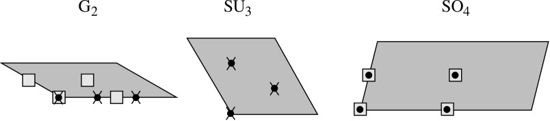
Figure 2: Fundamental region of the root lattice ${{\rm{G}_{2}}\oplus{\rm{SU}_{3}}\oplus{\rm{SO}_{4}}}$. The filled circles, crosses and squares represent fixed points in the $T_{1}$, $T_{2,4}$ and $T_{3}$ twisted sectors. See appendix B for further details.

There are three Kähler class moduli (${\cal T}_{1,2,3}$), whose real parts parameterize the sizes of the three tori, and one complex structure modulus (${\cal U}_{3}$), which parameterizes the shape of the third torus. Explicitly, ${\rm Re}{\cal T}_{3}=2RR^{\prime}\sin\phi$, and ${\cal U}_{3}=\frac{R}{R^{\prime}}\,{\rm e}^{{\rm i}\phi}$, where $R,R^{\prime}$ are the lengths of the two axes of the ${\rm{SO}_{4}}$-lattice and $\phi$ their relative angle. These moduli are arbitrary parameters. One may make the length of one axis (along which one puts the degree-2 Wilson line, ${\bf W}_{2}$), say $R$, large compared to the string length scale while keeping all other dimensions small. In this limit (for length scales larger than the string scale but smaller than the radius $R$), the low energy theory is effectively five dimensional. The ${\rm{SO}_{4}}$ lattice, on which only the ${\mathbb{Z}}_{2}$ sub-orbifold twist acts, has four fixed points. With only one degree-2 Wilson line, the fixed points split into two inequivalent classes, labelled by the winding number $n_{2}=0,1$. Thus in our setup the fifth dimension is equivalent to the orbicircle S${}^{1}/{\mathbb{Z}}_{2}$ where each of the two fixed points has a degree-2 degeneracy.

Note that we can reinterpret the ${\mathbb{Z}}_{6}$ models of appendix B in terms of the equivalent ${\mathbb{Z}}_{2}\times{\mathbb{Z}}_{3}$ orbifold (where the ${\mathbb{Z}}_{2}$ (${\mathbb{Z}}_{3}$) sub-orbifold twist acts on the ${\rm{G}_{2}}$ and ${\rm{SO}_{4}}$ (${\rm{G}_{2}}$ and ${\rm{SU}_{3}}$) sub-lattices). This point of view is more useful for our comparisons with the orbifold GUTs in sect. II.2. Labelling a twisted sector in the ${\mathbb{Z}}_{6}$ model by $T_{k}$ where $k=1,2,\cdots,5$ and in the ${\mathbb{Z}}_{2}\times{\mathbb{Z}}_{3}$ model by $T_{(k,l)}$ where $k=0,1$ and $l=0,1,2$, then the correspondence between the twisted sectors in the ${\mathbb{Z}}_{6}$ and ${\mathbb{Z}}_{2}\times{\mathbb{Z}}_{3}$ orbifolds is the following:

$$\begin{array}[]{l|lllll}\hline\cr{\mathbb{Z}}_{6}\ {\text{orbifold}}&T_{1}&T_{2}&T_{3}&T_{4}&T_{5}\\ \hline\cr{\mathbb{Z}}_{2}\times{\mathbb{Z}}_{3}\ {\text{orbifold}}&T_{(1,2)}&T_{(0,1)}&T_{(1,0)}&T_{(0,2)}&T_{(1,1)}\\ \hline\cr\end{array}\,.$$ (25)

The $T_{2,4}$ sectors, which will shortly be identified with the bulk states in the language of orbifold GUTs, have $k=0,\ l=1,2$; therefore they are untwisted by the ${\mathbb{Z}}_{2}$ twist.

III.1 Model A1 from the ${\mathbb{Z}}_{6}$ orbifold compactification

We now examine model A1 of appendix B. Consider first the model with only the ${\mathbb{Z}}_{3}$ sub-orbifolding being imposed (i.e., with twist vector ${\bf v}_{3}=2{\bf v}_{6}$, gauge twist ${\bf V}_{3}=2{\bf V}_{6}$ and a degree-3 Wilson line ${\bf W}_{3}$, where ${\bf v}_{6}$, ${\bf V}_{6}$ and ${\bf W}_{3}$ are given in eqs. 23, 84 and 86), we find a 6d ${\mathcal{N}}=2$ model with observable-sector gauge group E₆ (modulo abelian factors). Matter fields of the observable sector consist of 6d ${\mathcal{N}}=2$ hypermultiplets in the following representations,

$$U\,{\rm sectors}:\,{\bf 27}+{\bf\overline{27}},\qquad T\,{\rm sectors}:\,3\times({\bf 27}+{\bf\overline{27}})\,.$$ (26)

The remaining ${\mathbb{Z}}_{2}$ twist acts as a space reversal on the third compactified complex dimension, $Z_{3}\rightarrow-Z_{3}$. The ${\mathbb{Z}}_{3}$ models have two gravitini with the ${\rm{SO}_{8}}$ momentum vectors, ${\bf r}=\frac{1}{2}(1,1,1,1)$ and $\frac{1}{2}(1,-1,-1,1)$, in the Ramond sector of the right-moving superstring (see appendix A for notation). Only one of them, ${\bf r}=\frac{1}{2}(1,1,1,1)$, satisfies the ${\mathbb{Z}}_{2}$ projection, ${\bf r}\cdot{\bf v}_{2}={\mathbb{Z}}$. Hence the ${\cal N}=2$ supersymmetry is broken to that of ${\mathcal{N}}=1$ in 4d.

Gauge symmetry breaking induced by the ${\mathbb{Z}}_{2}$ orbifolding is as follows. The twist vector ${\bf v}_{2}$ is embedded in the gauge degrees of freedom in two different ways, with gauge twists ${\bf V}_{2}$ and ${\bf V}^{\prime}_{2}={\bf V}_{2}+{\bf W}_{2}$ where ${\bf V}_{2}=3{\bf V}_{6}$ and ${\bf W}_{2}$ is given in eq. 86. ${\rm{E}_{6}}$ generators in the Cartan-Weyl basis are transformed under the ${\mathbb{Z}}_{2}$ action as $E_{\bf P}\rightarrow{\rm e}^{2\pi{\rm i}{\bf P}\cdot{\bf V}_{2}}E_{\bf P}$ and $E_{\bf P}\rightarrow{\rm e}^{2\pi{\rm i}{\bf P}\cdot{\bf V}^{\prime}_{2}}E_{\bf P}$, thus the linearly-realized gauge groups consist of roots satisfying ${\bf P}\cdot{\bf V}_{2}$ and ${\bf P}\cdot{\bf V}^{\prime}_{2}={\mathbb{Z}}$ respectively. The pattern of symmetry breaking in the observable sector can be summarized as follows:

(27)

At the final step we have the complete ${\mathbb{Z}}_{6}$ model with two discrete Wilson lines being imposed simultaneously; this gives the PS symmetry group in the 4d effective theory.

In these two inequivalent implementations of the ${\mathbb{Z}}_{2}$ twist the non-trivial matter fields of ${\rm{SO}_{10}}$ and ${\rm{SU}_{6}}\times{\rm{SU}_{2R}}$ are:

$$\begin{array}[]{lll}\hline\cr{\rm Sectors}&{\rm{SO}_{10}}&{\rm{SU}_{6}}\times{\rm{SU}_{2R}}\\ \hline\cr U_{1}&{\bf 16}&({\bf 15,1})\\ U_{2}&{\bf 10}&({\bf 6,2})\\ U_{3}&{\bf 16}+{\bf\overline{16}}&({\bf 20,2})\\ T_{(0,1)}&2\times{\bf 16}_{+}+{\bf 10}_{-}&2({\bf\overline{6},2})_{+}+({\bf 15,1})_{-}\\ T_{(0,2)}&{\bf\overline{16}}_{-}+2\times{\bf 10}_{+}&({\bf 6,2})_{-}+2({\bf\overline{15},1})_{+}\\ \hline\cr\end{array}\,$$ (28)

where the subscripts $\pm$ represent intrinsic parities,

$$p=\gamma\phi\,.$$ (29)

$p$ depends on the twist eigenvalue, $\gamma$, and the oscillator phase, $\phi$; they are defined in appendix A. Note that $p=+$ for gauge and untwisted-sector states, and $p=+$ and $-$ have multiplicities $2$ and $1$ respectively for non-oscillator $T_{(01)}/T_{(02)}$ states.

Massless states in the untwisted and $T_{(0,1)},\,T_{(0,2)}$ twisted sectors of model A1 are the intersections of those of the ${\rm{SO}_{10}}$ and ${\rm{SU}_{6}}\times{\rm{SU}_{2R}}$ models. This can be seen from the group branching rules. For example, the $T_{(0,1)}$-sector matter has the following branchings,

$${\rm{SO}_{10}} \rightarrow \rm SU_{4C}\times SU_{2L}\times SU_{2R}$$

$${\bf 16}_{+} = ({\bf 4,2,1})_{+}+({\bf\overline{4},1,2})_{+}\,,$$

$${\bf 10}_{-} = ({\bf 6,1,1})_{-}+({\bf 1,2,2})_{-}\,,$$ (30)

$${\rm{SU}_{6}}\times{\rm{SU}_{2R}} \rightarrow \rm SU_{4C}\times SU_{2L}\times SU_{2R}$$

$$({\bf\overline{6},2})_{+} = ({\bf\overline{4},1,2})_{+}+({\bf 1,2,2})_{+}\,,$$

$$({\bf 15,1})_{-} = ({\bf 4,2,1})_{-}+({\bf 6,1,1})_{-}+({\bf 1,1,1})_{-}\,.$$ (31)

The states in common, $2({\bf\overline{4},1,2})_{+}+({\bf 6,1,1})_{-}$, agree with that of the $T_{2}$-twisted sector in eq. 89.

Massless fields in the other, i.e. $T_{(1,2)}(=T_{1})$ and $T_{(1,0)}(=T_{3})$, twisted sectors are the unions of those of the ${\rm{SO}_{10}}$ and ${\rm{SU}_{6}}\times{\rm{SU}_{2R}}$ models. Therefore there are two sets of states, furnishing complete representations of ${\rm{SO}_{10}}$ and ${\rm{SU}_{6}}\times{\rm{SU}_{2R}}$ respectively. For example, the $T_{1}$ sector of model A1 contains $({\bf 4,2,1})+({\bf\overline{4},1,2})$ and $({\bf 4,1,1})+({\bf 1,2,1})$, they are in the complete representations ${\bf 16}$ of ${\rm{SO}_{10}}$ and $({\bf 6,1})$ of ${\rm{SU}_{6}}\times{\rm{SU}_{2R}}$. In the notation of appendix A, these two sets of states have quantum numbers $n_{2}=0$ and $n_{2}=1$. (These quantum numbers are the winding numbers along the direction where the ${\bf W}_{2}$ Wilson line is imposed.) The $n_{2}=0$ and $n_{2}=1$ fixed points are thus the ${\rm{SO}_{10}}$ and ${\rm{SU}_{6}}\times{\rm{SU}_{2R}}$ branes in the orbifold GUT language.

III.2 Identifying orbifold parities in string theory

To a certain degree, the above ${\rm{E}_{6}}$ heterotic model gives a string theoretical realization of the orbifold GUT in sect. II.2. Better yet, we also achieve an understanding of the orbifold parities in terms of string theoretical quantities. Specifically, the analogue of orbifold parities, eq. 14, in our ${\mathbb{Z}}_{6}$ string models can be defined as follows KRZ0

$$P=p{\rm e}^{2\pi{\rm i}({\bf P}\cdot{\bf V}_{2}-{\bf r}\cdot{\bf v}_{2})}\,,\qquad P^{\prime}=p{\rm e}^{2\pi{\rm i}({\bf P}\cdot{\bf V}^{\prime}_{2}-{\bf r}\cdot{\bf v}_{2})}\,,$$ (32)

where ${\bf V}_{2}$ and ${\bf V}_{2}^{\prime}$ are the two inequivalent gauge embeddings of the ${\mathbb{Z}}_{2}$ twist in sect. III.1, and $p$ is the intrinsic parity.

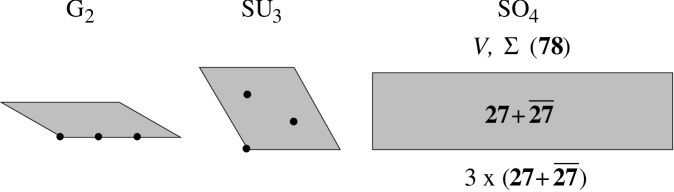
Figure 3: ${{\rm{G}_{2}}\oplus{\rm{SU}_{3}}\oplus{\rm{SO}_{4}}}$ lattice with ${\mathbb{Z}}_{3}$ fixed points. The fields $V,\ \Sigma,\$ and ${\bf 27}(\in U_{1})+{\bf\overline{27}}(\in U_{2})$ are bulk states from the untwisted sectors. On the other hand, $3\times({\bf 27}+{\bf\overline{27}})$ are “bulk” states located on the $T_{(0,1)}/T_{(0,2)}$ twisted sector (${\rm{G}_{2}}$, ${\rm{SU}_{3}}$) fixed points.

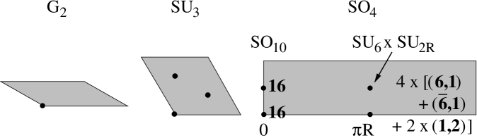
Figure 4: ${{\rm{G}_{2}}\oplus{\rm{SU}_{3}}\oplus{\rm{SO}_{4}}}$ lattice with ${\mathbb{Z}}_{6}$ fixed points. The $T_{(1,1)}/T_{(1,2)}$ twisted sector states sit at these fixed points.

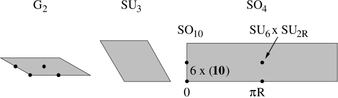
Figure 5: ${{\rm{G}_{2}}\oplus{\rm{SU}_{3}}\oplus{\rm{SO}_{4}}}$ lattice with ${\mathbb{Z}}_{2}$ fixed points. The $T_{(1,0)}$ twisted sector states sit at these fixed points.

These parities can be deduced from the generalized Gliozzi-Scherk-Olive (GSO) projector Gliozzi:1976qd ; IMNQ2 , as in the paragraphs after eq. 80. Since the terms in the exponents, ${\bf P}\cdot{\bf V}_{2}-{\bf r}\cdot{\bf v}_{2}$ and ${\bf P}\cdot{\bf V}^{\prime}_{2}-{\bf r}\cdot{\bf v}_{2}$, take integral or half-integral values, $P$ and $P^{\prime}$ are either $+$ or $-$. The orbifold translation corresponds to the difference in $P$ and $P^{\prime}$, i.e. $T={\rm e}^{2\pi{\rm i}{\bf P}\cdot{\bf W}_{2}}$. The $P$, $P^{\prime}$ and $T$ in string models have exactly the same properties as that of the orbifold GUTs.

Evidently, in the ${\rm{E}_{6}}$ orbifold GUT model of sect. II.2 states supported at the ${\rm{SO}_{10}}$ and ${\rm{SU}_{6}}\times{\rm{SU}_{2R}}$ branes are those with parities $P=+$ and $P^{\prime}=+$, and states in the 4d effective theory are those with parities $P=P^{\prime}=+$; this agrees with the string theoretical interpretation, since the parities in eq. 32 are nothing but the required GSO projections for the gauge, untwisted and $T_{(01)}/T_{(02)}$ sector states (i.e. the bulk states) in string models. (The massless states, i.e. $P=P^{\prime}=+$ modes from bulk and $T_{(0,1)}/T_{(0,2)}$ twisted sectors are shown in fig. 3.) From information gathered in sect. III.1 and appendix B, we can also deduce the $P$ and $P^{\prime}$ parities for the various bulk matter states. They are listed in table 1.

Table 1: Parities for the bulk states in model A1, computed from eq. 32. The states have been decomposed to the PS irreducible representations.

Multiplicities	States	$P$	$P^{\prime}$	States	$P$	$P^{\prime}$
1	$V({\bf 15,1,1})$	$+$	$+$	$\Sigma({\bf 15,1,1})$	$-$	$-$
1	$V({\bf 1,3,1})$	$+$	$+$	$\Sigma({\bf 1,3,1})$	$-$	$-$
1	$V({\bf 1,1,3})$	$+$	$+$	$\Sigma({\bf 1,1,3})$	$-$	$-$
1	$V({\bf 6,2,2})$	$+$	$-$	$\Sigma({\bf 6,2,2})$	$-$	$+$
1	$V({\bf 4,2,1})$	$-$	$+$	$\Sigma({\bf 4,2,1})$	$+$	$-$
1	$V({\bf\overline{4},1,2})$	$-$	$-$	$\Sigma({\bf\overline{4},1,2})$	$+$	$+$
1	$V({\bf\overline{4},2,1})$	$-$	$+$	$\Sigma({\bf\overline{4},2,1})$	$+$	$-$
1	$V({\bf 4,1,2})$	$-$	$-$	$\Sigma({\bf 4,1,2})$	$+$	$+$
1	$H({\bf 4,2,1})$	$+$	$+$	$H^{c}({\bf\overline{4},2,1})$	$-$	$-$
1	$H({\bf\overline{4},1,2})$	$+$	$-$	$H^{c}({\bf 4,1,2})$	$-$	$+$
1	$H({\bf 6,1,1})$	$-$	$+$	$H^{c}({\bf 6,1,1})$	$+$	$-$
1	$H({\bf 1,2,2})$	$-$	$-$	$H^{c}({\bf 1,2,2})$	$+$	$+$
2	$H({\bf 4,2,1})_{+}$	$+$	$-$	$H^{c}({\bf\overline{4},2,1})_{+}$	$-$	$+$
2	$H({\bf\overline{4},1,2})_{+}$	$+$	$+$	$H^{c}({\bf 4,1,2})_{+}$	$-$	$-$
2	$H({\bf 6,1,1})_{+}$	$-$	$-$	$H^{c}({\bf 6,1,1})_{+}$	$+$	$+$
2	$H({\bf 1,2,2})_{+}$	$-$	$+$	$H^{c}({\bf 1,2,2})_{+}$	$+$	$-$
1	$H({\bf 4,2,1})_{-}$	$-$	$+$	$H^{c}({\bf\overline{4},2,1})_{-}$	$+$	$-$
1	$H({\bf\overline{4},1,2})_{-}$	$-$	$-$	$H^{c}({\bf 4,1,2})_{-}$	$+$	$+$
1	$H({\bf 6,1,1})_{-}$	$+$	$+$	$H^{c}({\bf 6,1,1})_{-}$	$-$	$-$
1	$H({\bf 1,2,2})_{-}$	$+$	$-$	$H^{c}({\bf 1,2,2})_{-}$	$-$	$+$

KK masses for these bulk states can also be derived in string models. The mode expansions of the coordinates corresponding to the ${\rm{SO}_{4}}$ lattice are $X^{i}_{L,R}=x^{i}_{L,R}+p^{i}_{L,R}(\tau\pm\sigma)+{\rm oscillator\,terms}$, with $p^{i}_{L}$, $p^{i}_{R}$ given by eq. 69. The ${\mathbb{Z}}_{2}$ action maps $m$ to $-m$, $n$ to $-n$ and ${\bf W}_{2}$ to $-{\bf W}_{2}$, so physical states must contain linear combinations, $|m,n\rangle\pm|-m,-n\rangle$; the eigenvalues $\pm 1$ correspond to the first ${\mathbb{Z}}_{2}$ parity of the orbifold GUT models. The second embedding corresponds to a non-trivial Wilson line; it shifts the KK level by $m\rightarrow m+{\bf P}\cdot{\bf W}_{2}$. Since $2{\bf W}_{2}$ is a vector of the integral ${\rm{E}_{8}}\times{\rm{E}_{8}}$ lattice, the shift ${\bf P}\cdot{\bf W}_{2}$ must be an integer or half-integer. In the orbifold GUT limit when the winding modes and the KK modes in the short direction of ${\rm{SO}_{4}}$ decouple, eq. 69 reproduces the field theoretical mass formula in eq. 5.

As seen in sect. III.1, matter states in the $T_{(1,1)}/T_{(1,2)}$ and $T_{(1,0)}$ twisted sectors, which may be identified with the first two families, are localized on the two inequivalent fixed points in the ${\rm{SO}_{4}}$ lattice. They are the ${\rm{SO}_{10}}$ and ${\rm{SU}_{6}}\times{\rm{SU}_{2R}}$ brane states (See figs. 4 and 5). These twisted-sector states are more tightly constrained than their orbifold GUT counterparts. In orbifold GUT models the only consistency requirement is the chiral anomaly cancellation, thus one can add arbitrary numbers of vector-like representations to the branes. String models have to satisfy more stringent modular invariance conditions Dixon ; vafa (of course, one-loop modular invariance guarantees the model is anomaly free, up to a possible anomalous abelian factor LSW ), which also constrains any additional matter in vector-like representations.

III.3 Other models

In this subsection, we discuss the other two models in appendix B in the orbifold GUT language, for completeness. These models do not have matter-Higgs couplings at the renormalizable level, and may have limited phenomenological interest.

Model A2 has already been analyzed in ref. KRZ0 . In the 5d bulk, it has an ${\rm{SO}_{10}}\times{\rm{SU}_{2}}$ gauge symmetry and the following set of matter states,

$$U\,{\rm sectors}:({\bf 16,1})+({\bf 1,2}),\qquad T\,{\rm sectors}:3({\bf 16,1})+6({\bf 10,1})+15({\bf 1,2})\,.$$ (33)

The bulk gauge group is unbroken at the fixed point $x^{5}=0$ and broken to the PS group at $x^{5}=\pi R$ respectively, the states supported at these two points are

$$\begin{array}[]{lll}\hline\cr{\rm Sectors}&{\rm{SO}_{10}}\times{\rm{SU}_{2}}&{\rm PS}\\ \hline\cr U_{1}&({\bf 16,1})&({\bf 4,2,1})\\ U_{2}&({\bf 1,2})&({\bf 4,1,2})\\ U_{3}&-&({\bf 6,2,2})\\ T_{(0,1)}&2({\bf 16,1})_{+}+2({\bf 10,1})_{-}&({\bf 6,1,1})_{-}+2({\bf 1,2,2})_{+}\\ &+2({\bf 1,2})_{+}+4({\bf 1,2})_{-}&+2({\bf 6,1,1})_{+}+({\bf 1,2,2})_{-}\\ &&+({\bf 4,2,1})_{-}+2({\bf\overline{4},1,2})_{+}\\ T_{(0,2)}&({\bf\overline{16},1})_{-}+4({\bf 10,1})_{+}&2({\bf 6,1,1})_{+}+({\bf 1,2,2})_{-}\\ &+8({\bf 1,2})_{+}+({\bf 1,2})_{-}&+({\bf 6,1,1})_{-}+2({\bf 1,2,2})_{+}\\ &&+({\bf 4,1,2})_{-}+2({\bf\overline{4},2,1})_{+}\\ \hline\cr\end{array}\,.$$ (34)

Model B is similar to model A1, with an ${\rm{E}_{6}}$ bulk group and the same set of bulk states as in eq. 26. The ${\rm{E}_{6}}$ group is broken to ${\rm{SO}_{10}}$ and ${\rm{SU}_{6}}\times{\rm{SU}_{2L}}$ respectively at the two fixed points, and the matter states are

$$\begin{array}[]{lll}\hline\cr{\rm Sectors}&{\rm{SO}_{10}}&{\rm{SU}_{6}}\times{\rm{SU}_{2L}}\\ \hline\cr U_{1}&{\bf\overline{16}}&({\bf 6,2})\\ U_{2}&{\bf 10}&({\bf 15,1})\\ U_{3}&{\bf 16}+{\bf\overline{16}}&({\bf 20,2})\\ T_{(0,1)}&2\times{\bf\overline{16}}_{+}+{\bf 10}_{-}&({\bf 6,2})_{-}+2({\bf\overline{15},1})_{+}\\ T_{(0,2)}&{\bf 16}_{-}+2\times{\bf 10}_{+}&2({\bf\overline{6},2})_{+}+({\bf 15,1})_{-}\\ \hline\cr\end{array}\,.$$ (35)

The 4d effective theories of models A2 and B have a PS symmetry, and the complete matter content is listed in appendix B. Similar to model A1, matter fields in the untwisted and $T_{2}/T_{4}$ twisted sectors can be traced back to the states in the above two tables, by using appropriate group branching rules. We also note that both models contain two families of chiral matter from the fixed point at $x^{5}=0$ and one family from the bulk, a common feature to all our models. This feature predicts a non-abelian dihedral ${\rm{D}_{4}}$ family symmetry – a novelty in string model building – as we will see in the next section.

III.4 The color-triplet problem

A major motivation for constructing orbifold GUT models is the well-known doublet-triplet splitting problem in conventional 4d GUTs. Orbifold GUTs solve this problem by assigning appropriate orbifold parities to the Higgs doublets and triplets, such that the triplets are automatically projected out of the effective theory kawamura . We have already seen this in the ${\rm{SO}_{10}}$ model in sect. II.1. This mechanism, however, usually cannot be trivially implemented in heterotic models.

The difficulty is largely due to the intricate nature of string models. These models need to satisfy delicate modular invariance consistency conditions Dixon ; vafa and are physically more constrained than the orbifold GUTs. Before imposing any Wilson line, the ${\mathbb{Z}}_{6}$ models of eqs. 84 and 85 always contain the ${\bf 10}$ representation of ${\rm{SO}_{10}}$ simultaneously in several sectors. We find it is impossible to design modular-invariant Wilson lines to fulfill the following requirements: (a) break the gauge group to PS in 4d, (b) give rise to three chiral families, and (c) eliminate the color triplets altogether. Furthermore, the ${\bf 10}$ representation of the $T_{3}$ sector in model A1 does not suffer from additional projections even when the ${\bf W}_{2}$ Wilson line is turned on. Indeed, it simply decomposes to the $({\bf 6},{\bf 1},{\bf 1})+({\bf 1},{\bf 2},{\bf 2})$ representations under the PS group.

Although the presence of many color triplets is a nuisance, one ${\bf 3}+{\bf\overline{3}}$ pair may be necessary to facilitate the breaking of PS to the SM gauge group, as illustrated in the E₆ model in sect. II.2. Moreover, it is not entirely clear that the color triplets in our models pose the same problems as in conventional GUTs. Indeed, although there are color triplets (those of the $T_{1}$/$T_{3}$ twisted sectors) with doublet companions having exactly the same quantum numbers, in general we also have $({\bf 6,1,1})$ and $({\bf 1,2,2})$ states with different quantum numbers, in all three models. The usual doublet-triplet problem does not necessarily apply for the second situation. We need to check whether it is possible to make all color triplets sufficiently heavy while (hopefully) keeping one MSSM Higgs-doublet pair light; this requires a better understanding of the effective actions of our models and will be examined for model A1 in the next section.

IV Phenomenology of model A1

We have seen in the previous sections that the E₆ orbifold GUT and heterotic A1 model match nicely in the low energy regime. In this section, we study some phenomenological issues for the A1 model. We first study gauge coupling unification, relying on a simplification due to the correspondence between the field and string theoretical models. We then study Yukawa couplings (including both renormalizable and non-renormalizable couplings), concentrating on several immediate phenomenological questions: (i) breaking of the PS symmetry to that of the SM, (ii) mass generation for the color triplets, (iii) proton stability, and (iv) matter-Higgs Yukawa couplings. These couplings are introduced by hand in the orbifold GUTs. In string models we no longer enjoy the same kind of freedom. In fact, these couplings are determined by string selection rules (reviewed in appendix C.1). The low energy phenomenology also depends crucially on the flat directions of the effective ${\mathcal{N}}=1$ model. However, we do not attempt to solve this complicated problem here.

IV.1 Gauge coupling unification and proton decay

As discussed earlier, since the first two families are located on the ${\rm{SO}_{10}}$ brane, proton decay constraints require that the 5d compactification scale $M_{c}$ be greater than $O(10^{16})$ GeV. However all these GUT scale thresholds must be consistent with low energy gauge coupling unification. Consider the solution to the 5d renormalization group (RG) equations, i.e., the GQW equations, in the orbifold GUT limit, given by

$$\frac{2\pi}{\alpha_{i}(\mu)} \simeq \frac{2\pi}{\alpha_{\rm string}}+b^{\rm MSSM}_{i}\log\frac{M_{\rm PS}}{\mu}+(b^{\rm PS}_{++}+b_{\rm brane})_{i}\log\frac{{M_{\rm string}}}{M_{\rm PS}}$$ (36)

$$- \frac{1}{2}(b^{\rm PS}_{++}+b^{\rm PS}_{--})_{i}\log\frac{{M_{\rm string}}}{M_{c}}+b^{{\rm E}_{6}}\left(\frac{{M_{\rm string}}}{M_{c}}-1\right),$$

where $M_{\rm PS}$ is the PS breaking scale and $\alpha_{\rm string}$ is the gauge coupling at the string scale. In addition, in the weakly coupled heterotic string we have the boundary condition

$$\frac{2\pi}{\alpha_{\rm string}}=\frac{\pi}{4}\left(\frac{M_{\rm Pl}}{M_{\rm string}}\right)^{2}+\frac{1}{2}\ \Delta^{\rm univ},$$ (37)

where the first term is the tree level result and the second is a universal one loop stringy correction. The latter correction depends on the value of the ${\cal T}_{3},\ {\cal U}_{3}$ moduli. Following ref. KL we see that $\Delta^{\rm univ}$ is a finite function of its argument (with a mild singularity when ${\cal T}_{3}={\cal U}_{3}$, modulo PSL$(2,{\mathbb{Z}})$ transformations). Since the universal correction is not significant, we use the tree level formula in the following.

Eq. 36 can be compared mathematically to the 4d equations given by

$$\frac{2\pi}{\alpha_{i}(\mu)}\simeq\frac{2\pi}{\alpha_{\rm GUT}}+b^{\rm MSSM}_{i}\log\frac{M_{\rm GUT}}{\mu}+6\;\delta_{i3},$$ (38)

where $M_{\rm GUT}\simeq 3\times 10^{16}$ GeV, $\alpha_{\rm GUT}^{-1}\simeq 24$ and we have included a threshold correction at $M_{\rm GUT}$, required in order to fit the low energy data.

With the bulk field parities given in table 1, we find the beta function coefficients, $\frac{1}{2}(b_{++}^{\rm PS}+b_{--}^{\rm PS})=(1,1,1)$, $\;\;b_{++}^{\rm PS}=(\frac{9}{5},-3,-3)$. The brane contributions include that of the two PS families, $b_{\rm brane}=(4,4,4)$, and those from extra matter fields, $n^{\prime}_{{\bf 6}+{\bf\overline{6}}}(\frac{2}{5},1,1)+n_{\bf 10}(1,1,1)+n^{\prime}_{{\bf 2}_{R}}(\frac{3}{10},0,0)$ (with $n^{\prime}_{{\bf 6}+{\bf\overline{6}}}\leq 4$, $n_{\bf 10}\leq 6$ and $n^{\prime}_{{\bf 2}_{R}}\leq 12$). Equating the difference $2\pi/\alpha_{3}(\mu)-2\pi/\alpha_{2}(\mu)$, eqs. 36 and 38 gives

$$M_{\rm PS}\simeq{\rm e}^{-3/2}M_{\rm GUT}\simeq 7\times 10^{15}\ {\rm GeV}.$$ (39)

Then equating the difference $2\pi/\alpha_{2}(\mu)-2\pi/\alpha_{1}(\mu)$, we find

$$\log\frac{M_{\rm string}}{M_{\rm GUT}}\simeq\frac{8-3n^{\prime}_{{\bf 2}_{R}}+6n^{\prime}_{\bf 6+\overline{6}}}{32+2n^{\prime}_{{\bf 2}_{R}}-4n^{\prime}_{\bf 6+\overline{6}}},$$ (40)

which results in a maximum value for $M_{\rm string}$ for $n^{\prime}_{{\bf 2}_{R}}=0$, $n^{\prime}_{\bf 6+\overline{6}}=4$, given by

$$M_{\rm string}^{\rm max}\simeq{\rm e}^{2}M_{\rm GUT}\simeq 2\times 10^{17}\ {\rm GeV}.$$ (41)

Finally we have

$$\frac{\alpha_{\rm GUT}}{\alpha_{\rm string}}-1\simeq\frac{\alpha_{\rm GUT}}{2\pi}\left[\log\frac{M_{\rm GUT}}{M_{c}}-(n_{10}+n^{\prime}_{\bf 6+\overline{6}})\left(\log\frac{M_{\rm string}}{M_{\rm GUT}}+\frac{3}{2}\right)\right].$$ (42)

Using $M_{\rm string}=M_{\rm string}^{\rm max}$ and eq. 37 for the tree level heterotic string boundary condition, we find there is no solution, consistent with $M_{\rm string}>M_{c}\simeq M_{\rm GUT}>M_{\rm PS}$. The problem is that the value of $\alpha_{\rm string}$ given by eq. 37 is much too small ($\alpha_{\rm string}\ll\alpha_{\rm GUT}$) and it cannot be obtained by logarithmic running above the compactification scale (note, $b^{{\rm{E}_{6}}}=0$ and thus there is no power-law running). This problem suggests that non-trivial (perhaps non-perturbative) string boundary conditions are required for consistency.

We have considered the 11d Hořava-Witten extension hw of the perturbative heterotic string boundary condition given by witten

$$\frac{2\pi}{\alpha_{\rm string}}=\frac{1}{2(4\pi)^{5/3}M_{*}\rho}\ \left(\frac{M_{\rm Pl}}{M_{*}}\right)^{2},$$ (43)

where $M_{*}$ is given in terms of the 11d Newton’s constant by $\kappa^{2/3}=M_{*}^{-3}$ and $\rho$ is the size of the eleventh dimension. Now using eq. 43, we find solutions for $M_{\rm string}\simeq M_{*}=2M_{\rm GUT},\;M_{c}\simeq M_{\rm PS}\simeq{\rm e}^{-3/2}M_{\rm GUT}$ with $n^{\prime}_{{\bf 2}_{R}}=n^{\prime}_{\bf 6+\overline{6}}=4$ and $M_{*}\rho\simeq 2$. Of course, this solution provides an enhanced proton decay rate due to dimension-6 operators with the dominant decay mode $p\rightarrow e^{+}\pi^{0}$. The decay rate for dimension-6 operators is given by pdecay

$$\tau(p\rightarrow e^{+}\pi^{0}) \simeq 1.25\times 10^{36}\;\left(\frac{M_{X}}{3\times 10^{16}\ {\rm GeV}}\right)^{4}\;\left(\frac{0.015\ {\rm GeV}^{3}}{\beta_{\rm lattice}}\right)^{2}\;\;{\rm yrs}$$ (44)

$$\simeq 3\times 10^{33}\;\left(\frac{0.015\ {\rm GeV}^{3}}{\beta_{\rm lattice}}\right)^{2}\;\;{\rm yrs},$$

where $\beta_{\rm lattice}$ is an input from lattice calculations of the three quark matrix element. Recent results give a range of central values $\beta_{\rm lattice}=0.007-0.015$ lattice . Note, the present experimental bound for this decay mode from Super-Kamiokande is $5.7\times 10^{33}$ years at $90\%$ confidence levels superk . Thus this prediction is not yet excluded by the data, but it should be observed soon.

IV.2 Yukawa couplings

IV.2.1 PS symmetry breaking, mass generation for color-triplets and proton stability

To successfully break the PS symmetry to that of the SM and generate mass for unwanted color triplet states, the 5d ${\rm{E}_{6}}$ heterotic model should contain non-trivial couplings of the form in eq. 22. The model, however, contains additional color triplets. They could, in principle, develop mass through non-trivial Yukawa couplings to, say, singlet fields. In order to verify if this is a possibility, we need to know whether the required couplings exist in the 4d effective theory of the string model. For this purpose we are particularly interested in non-trivial couplings containing PS invariant operators, $({\bf 6,1,1})({\bf 6,1,1})$, $({\bf 6,1,1})({\bf 4,1,2})({\bf 4,1,2})$ and $({\bf 6,1,1})({\bf\overline{4},1,2})({\bf\overline{4},1,2)}$, that are allowed by string selection rules. (In field theory, all gauge invariant operators would be allowed.) These rules are reviewed in appendix C.1 and the relevant operators are given in eqs. 105 – 108.

Cubic, renormalizable, couplings in model A1 are determined in eq. 103, they contain the following operators of interest (we label the fields according to table 2),

$${\cal W}^{(3)}\supset S_{1}(C_{3})_{A\alpha}(C_{3})_{B\beta}+C_{1}\overline{\chi}_{1}^{c}\overline{\chi}_{2}^{c}+(C_{3})_{A\alpha}f^{c}_{B}\chi^{c}_{\beta}+(C_{4})_{\alpha}\chi^{c}_{\beta}f_{3}^{c}+(C_{4})_{\alpha}f_{A}^{c}f_{B}^{c},$$ (45)

where $\alpha,\beta=1,2$ labels the two $\gamma=1$ eigenstates in the $T_{2,4}$ sectors, $A,B=1,2$ indicate degeneracies associated with the $n^{\prime}_{2}$ winding number (which corresponds to a hidden ${\rm{S}_{2}}$ permutation symmetry). The string selection rules require $\alpha+\beta=0\,{\rm mod}\,2$, $A+B=0\,{\rm mod}\,2$, and for the last term $\alpha$ is unrestricted. Apparently these couplings are not sufficient to break the PS symmetry and give mass to all the color triplets contained in the $({\bf 6,1,1})$ and $({\bf 4,1,2})+({\bf\overline{4},1,2})$ states. Thus, to achieve our goal, we must also take into consideration higher-dimensional operators. Some of them are listed in appendix C.2. (Of course, there are many more operators with even higher dimensions. It is not obvious that “stringy zeroes” exist. We omitted these operators. They may or may not disrupt the following discussion.)

A few observations are appropriate. The fields $C_{i}$, $i=1,\cdots,4$ transform as a ${\bf 3}_{-2/3}+{\bf\overline{3}}_{2/3}$ under ${\rm{SU}_{3C}}\times{\rm{U}_{1Y}}$ or as $\overline{D}^{c}+\overline{D}$ where $\overline{D}$ has the quantum number of an anti-down quark. These color triplets have multiplicities [in brackets], $C_{1}[1],\ C_{2}[2],\ C_{3}[4],\ C_{4}[2]$. In addition $C_{2},\ C_{3}$ appear in complete ${\rm{SO}_{10}}$ 10-plets. We also have states contained in $\chi^{c}_{\alpha},\ \overline{\chi}^{c}_{1,2}$ with quantum numbers of $\overline{D},\ \overline{D}^{c},\ \overline{U},\ \overline{U}^{c},\ \overline{E},\,\overline{E}^{c}$. Finally we have the color triplet states in $q_{1},\ q_{2},\ \overline{q}_{1},\ \overline{q}_{2}$ with multiplicity 2 each. These latter are exotic states with fractional charge $\pm 1/2$ for the color singlets and $\pm 1/6$ for the color triplets.

For the exotic states we find operators of the form $\overline{q}_{1}(q_{1}+q_{2})$ multiplied by products of singlets $S^{n}$ (up to sixth order), but no operators of the form $\overline{q}_{2}(q_{1}+q_{2})S^{n}$ to order $n=9$. Hence $\overline{q}_{2}$ and one linear combination of $q_{1},\ q_{2}$ remain massless. This is a serious problem for the model, since these states are absolutely stable and should have been observed. It remains to be seen whether the operator $\overline{q}_{2}(q_{1}+q_{2})S^{n}$ is generated at order $n\geq 10$ or if it is forbidden by the string selection rules to all orders.

Now consider the fields $C_{i}$, $i=1,\cdots,4$ and $\chi^{c}_{\alpha},\ \overline{\chi}^{c}_{1,2}$. In this sector we need to both find a way of spontaneously breaking PS to the SM, as well as giving all color triplets mass. A related issue is the potential problem of rapid proton decay mediated by these color triplets. In particular we must eliminate or greatly suppress the following baryon/lepton-number violating effective operators

$$fff^{c}\langle\chi^{c}S^{n}\rangle\Longrightarrow QL\overline{D}+LL\overline{E},\qquad f^{c}f^{c}f^{c}\langle\chi^{c}S^{n}\rangle\Longrightarrow\overline{U}\,\overline{D}\,\overline{D}.$$ (46)

Note we have checked that these operators are not generated prior to integrating out the color triplets, for $n\leq 3$. Nevertheless there is a danger that they will be generated in the effective theory below the color triplet mass. In fact, consider the renormalizable couplings in eq. 45. It is evident that an effective mass term of the form $\langle S\rangle(C_{4})^{2}$ combined with the coupling $C_{4}(\chi^{c}_{\alpha}f_{3}^{c}+f_{A}^{c}f_{B}^{c})$ leads to the effective operator of the form

$$\frac{1}{\langle S\rangle}\chi^{c}_{\alpha}f_{3}^{c}f_{A}^{c}f_{B}^{c}=\frac{M_{\rm PS}}{\langle S\rangle}\overline{U}_{3}\overline{D}_{A}\overline{D}_{B}.$$ (47)

Similarly, additional baryon/lepton-number violating operators are obtained from an effective $C_{3}C_{4}$ mass term. These baryon-number violating operator may be phenomenologically acceptable if the coefficient is sufficiently small. However it seems prudent to eliminate the offending mass terms by choosing a vacuum configuration where the appropriate scalar vevs vanish. For example, given the superpotential terms in appendix C, eq. 105, we demand that the following vevs (i.e. the coefficients of $(C_{4})^{2}$ and $C_{3}C_{4}$) vanish $S_{2}S_{24}+{\cal S}_{1}^{(2)}{\cal S}_{2}^{(2)}={\cal S}^{(2)}_{1}+S_{2}S_{9}S_{24}+S_{1}{\cal S}^{(2)}_{2}+S_{19}S_{25}{\cal S}^{(2)}_{2}=0$.

In the following we consider the possibility of obtaining a baryon/lepton-number conserving low energy effective theory. As a possible proof of existence, we suggest an ansatz where the only singlets with non-vanishing vevs are

$$\{S_{1}\},\quad\{S_{10}{\cal S}_{4}^{(2)}\},\quad[S_{6}S_{7}S_{14}S_{18}],\quad[S_{7}S_{14}S_{16}(S_{6}S_{26}+S_{2}S_{27})],\quad\{S_{26}\},$$ (48)

where the curly braces represent classes of singlets with the same transformation properties under all string symmetries and we use square brackets when we explicitly present a finite set of fields in the same class. The corresponding superpotential from appendix C.2 is

$${\cal W} \supset \,\,\,\,\biggr{(}\{S_{1}\}(C_{3})^{2}+\{S_{2}S_{22}{\cal S}_{9}^{(2)}\}C_{2}C_{3}+\{S_{10}{\cal S}_{4}^{(2)}\}C_{1}C_{4}\biggr{)}$$ (49)

$$+\biggr{(}C_{1}\overline{\chi}_{1}^{c}\overline{\chi}_{2}^{c}+C_{3}f^{c}_{A}\chi^{c}_{\alpha}+C_{4}(\chi^{c}_{\alpha}f_{3}^{c}+f_{A}^{c}f_{B}^{c})\biggr{)}$$

$$+\biggr{(}\{S_{2}S_{24}S_{26}\}C_{4}(\overline{\chi}_{1}^{c})^{2}+[S_{10}{\cal S}_{1}^{(2)}+S_{6}S_{7}S_{14}S_{18}+S_{1}S_{10}{\cal S}^{(2)}_{2}+S_{2}{\cal S}^{(3)}_{4}]C_{4}(\overline{\chi}_{2}^{c})^{2}$$

$$\qquad+[S_{2}S_{3}S_{12}{\cal S}_{3}^{(2)}+S_{7}S_{14}S_{16}(S_{6}S_{26}+S_{2}S_{27})]C_{4}\chi_{\alpha}^{c}\chi_{\beta}^{c}\biggr{)}+\{S_{26}\}\chi_{\alpha}^{c}\overline{\chi}_{1}^{c}.$$

Note the coefficient of the $C_{2}C_{3}$ term and the first term linear in $C_{4}$ vanishes due to the vevs we have chosen, but there may be other higher-dimensional terms which replace them. For example, the first element in the second term linear in $C_{4}$ also vanishes, but the other terms may be non-zero.

The following vevs are assumed to vanish.

$$[S_{2}S_{24}+{\cal S}_{1}^{(2)}{\cal S}_{2}^{(2)}], [{\cal S}^{(2)}_{1}+S_{2}S_{9}S_{24}+S_{1}{\cal S}^{(2)}_{2}+S_{19}S_{25}{\cal S}^{(2)}_{2}],$$ (50)

$$\{S_{2}S_{9}S_{22}\}, [S_{10}{\cal S}^{(2)}_{3}+S_{13}{\cal S}^{(2)}_{2}+S_{1}S_{10}S_{12}S_{32}+S_{9}S_{10}{\cal S}^{(2)}_{4}],$$

$$\{S_{9}\}\equiv S_{9}+S_{1}S_{10}S_{21}S_{22}+{\cal S}^{(2)}_{2}S_{11}^{2}+\cdots, [{\cal S}_{9}^{(2)}+S_{10}(S_{30}{\cal S}^{(2)}_{5}+S_{13}{\cal S}^{(2)}_{4})],$$

$$[{\cal S}^{(2)}_{2}+S_{26}{\cal S}^{(3)}_{2}], [S_{9}{\cal S}_{9}^{(2)}+S_{13}(S_{10}{\cal S}^{(2)}_{3}+S_{13}{\cal S}^{(2)}_{2})],$$

$$\{S_{10}S_{13}S_{21}S_{22}\}, \{S_{9}S_{10}S_{12}S_{32}\},\qquad\{S_{10}{\cal S}_{1}^{(3)}\}$$

With this choice we guarantee, at least to the order we have checked, that we do not generate baryon/lepton-number violating operators in the low energy theory obtained by integrating out the color triplets. A self-consistent solution to the necessary set of vevs is given by

$$S_{4}=S_{9}=S_{11}=S_{13}=S_{17}=S_{21}=S_{24}=S_{25}=S_{29}=S_{30}=S_{32}=0,$$ (51)

and all other vevs non-zero. In addition we require $[S_{5}S_{33}+S_{10}S_{26}]=0$, which may or may not require fine-tuning. Unfortunately we are not able to identify a symmetry which would extend this result to all orders in string perturbation. This is a serious problem for the model.

The first term in parentheses of eq. 49 gives mass to the color triplets $C_{2}$, $C_{3}$, $C_{1}$ and one triplet in $C_{4}$. Since the doublets $h_{2}$ and $h_{3}$ have exactly the same quantum numbers as that of $C_{2}$ and $C_{3}$, they acquire the same mass and also decouple from the low energy effective theory. In this way, we obtain just one doublet field $h_{1}$ (from the $U_{2}$ sector). It is a good candidate for the MSSM Higgs-doublet pair.

The last term of eq. 49 is in the form of eq. 22, with two pairs of $\chi^{c}+\overline{\chi}^{c}$ fields. With $\langle S_{26}\rangle\neq 0$ an F-flat solution is found with $\langle\chi_{1}^{c}\rangle=\langle\overline{\chi}^{c}_{1}\rangle=0$, then this part of the superpotential reduces to eq. 22. Employing F and D flatness conditions, the potential has a flat direction along the right-handed-neutrino direction of $\chi_{2}^{c}+\overline{\chi}_{2}^{c}$, as in eq. 20. The non-vanishing vevs break the PS to the SM gauge group and subsequently gives mass to the remaining massless color triplets in $C_{4}$ and the $D^{c}+\overline{D}^{c}$ components in $\chi^{c}_{2}+\overline{\chi}^{c}_{2}$. The remaining charged states in $\chi^{c}_{2}+\overline{\chi}^{c}_{2}$ obtain mass via the super-Higgs mechanism. Lastly, the $\chi^{c}_{1}+\overline{\chi}^{c}_{1}$ also acquire mass via the $\langle S_{26}\rangle$ vev in eq. 49.

The remaining central problem is whether the required singlets, such as those in eq. 48, could develop the appropriate vevs along F- and D-flat directions. There are five abelian factors in the A1 model, one of them is anomalous (which is cancelled by the generalized Green-Schwarz mechanism GS ; au1 , as usual). In general, the anomalous ${\rm{U}_{1}}$ factor destabilizes the original vacua and contributes vevs to some of the singlet fields. It requires further investigation to determine whether our assumptions in the previous paragraph are substantiated, and moreover whether all the abelian symmetries may be broken with the vacuum solution. (The ${\mathcal{N}}=1$ supersymmetry, however, is generically preserved in the effective theory.) Refs. FIQS ; GCEEL have already obtained some necessary conditions for analyzing non-trivial singlet vevs. We leave a detailed investigation for the future.

IV.2.2 ${\rm{D}_{4}}$ family symmetry

Before discussing the Yukawa matrices for quarks and leptons, we consider the family symmetry of model A1. The third family is a bulk field, while the first two families are located on the two $\mathbb{Z}_{2}$ fixed points in the ${\rm{SO}_{4}}$ torus with an ${\rm{SO}_{10}}$ gauge symmetry. One family sits at each fixed point (see fig. 4). Since the Wilson line in the ${\rm{SO}_{4}}$ torus lies in the orthogonal direction to these two fixed points, the theory is invariant under the permutation of the first two families, labelled by an index $n_{2}^{\prime}=0,1$ (or $A=1,2$). In addition, the string selection rule, eq. 100, requires that every effective fermion mass operator include an even number of fields with $n_{2}^{\prime}=1$. Hence these effective operators are invariant under a $\mathbb{Z}_{2}$ parity $n^{\prime}_{2}\rightarrow-n^{\prime}_{2}$. The two operations are generated by the two Pauli matrices $\sigma_{1}=\left(\begin{array}[]{cc}0&1\\ 1&0\end{array}\right)$ and $\sigma_{3}=\left(\begin{array}[]{cc}1&0\\ 0&-1\end{array}\right)$ acting on a real two dimensional vector. The complete set of operations closes on the discrete non-abelian family symmetry group ${\rm{D}_{4}}=\{\pm I,\ \pm\sigma_{1},\ \pm\sigma_{3},\ \mp{\rm i}\sigma_{2}\}$. Note that the eight-element finite (dihedral) group ${\rm{D}_{4}}$ is the symmetry group of a square. It has five conjugacy classes and five faithful representations. The character table is

$$\begin{array}[]{lrrrrr}\hline\cr{\rm Classes}&I&-I&\pm\sigma_{1}&\pm\sigma_{3}&\mp{\rm i}\sigma_{2}\\ \hline\cr{\rm Doublet}-D&2&-2&0&0&0\\ {\rm Singlet}-A_{1}&1&1&1&1&1\\ {\rm Singlet}-B_{1}&1&1&1&-1&-1\\ {\rm Singlet}-B_{2}&1&1&-1&1&-1\\ {\rm Singlet}-A_{2}&1&1&-1&-1&1\\ \hline\cr\end{array}.$$ (52)

In our models, the first two families transform as the doublet, while the third family transforms as the trivial singlet.

We have many ${\rm{SO}_{10}}$ singlets in our models, transforming as doublets under ${\rm{D}_{4}}$. They appear in effective higher dimension fermion mass operators. Consider, for example, two doublets under ${\rm{D}_{4}}$ given by {$S_{A},\tilde{S}_{A}$}. Then in terms of these two doublets we can define bilinear combinations transforming as {$A_{1},A_{2},B_{1},B_{2}$}. We have

$$S_{1}\tilde{S}_{1}+S_{2}\tilde{S}_{2}\sim A_{1}$$

$$S_{1}\tilde{S}_{2}-S_{2}\tilde{S}_{1}\sim A_{2}$$

$$S_{1}\tilde{S}_{2}+S_{2}\tilde{S}_{1}\sim B_{1}$$

$$S_{1}\tilde{S}_{1}-S_{2}\tilde{S}_{2}\sim B_{2}$$ (53)

The effective Yukawa couplings are then constructed in terms of ${\rm{D}_{4}}$ invariants. Define the ${\rm{D}_{4}}$ doublet left-handed quarks and leptons $({\bf 4,2,1})$ [$=f_{A}$] and left-handed anti-quarks and anti-leptons $({\bf\bar{4},1,2})$ [$=f^{c}_{A}$] for the first two families and the Higgs multiplet $({\bf 1,2,2})$ [$=h$]. We then have the PS and ${\rm{D}_{4}}$ invariants:

$$hA_{1}(f_{1}f^{c}_{1}+f_{2}f^{c}_{2})\equiv hA_{1}(f_{A}f^{c}_{A})$$

$$hA_{2}(f_{1}f^{c}_{2}-f_{2}f^{c}_{1})$$

$$hB_{1}(f_{1}f^{c}_{2}+f_{2}f^{c}_{1})$$

$$hB_{2}(f_{1}f^{c}_{1}-f_{2}f^{c}_{2})$$ (54)

We can also have operators of the form

$$h(f_{A}S_{A})(f^{c}_{B}S_{B})=h[f_{1}f^{c}_{1}S_{1}^{2}+f_{2}f^{c}_{2}S_{2}^{2}+(f_{1}f^{c}_{2}+f_{2}f^{c}_{1})S_{1}S_{2}]$$ (55)

Unfortunately there are, in principle, several possible ways of constructing ${\rm{D}_{4}}$ invariants. We are not able to determine, without further string calculations, how to contract the ${\rm{D}_{4}}$ indices. In the following we assume, for illustrative purposes, that only the simplest invariants, $A_{1}$ and $B_{1}$, appear in the effective Yukawa couplings.

IV.2.3 Fermion masses

The only Yukawa coupling in model A1 present at leading order is for the third family, given by the first term in eq. 103. From discussions in sect. II.2, we conclude that this coupling unifies with the GUT gauge coupling at the 5d compactification scale, as in eq. 17. Yukawa couplings for the first two families come from higher-dimensional non-renormalizable operators. In addition they are constrained by the ${\rm{D}_{4}}$ family symmetry. In principle, there are at least two possible types of operators. The first type involves operators of the form $h_{1}(f_{3}f_{A}^{c},\ f_{A}f_{3}^{c},\ f_{A}f_{B}^{c})$, multiplied by suitable singlets, and the second type also involves composite singlets $\overline{\chi}^{c}\chi^{c}$. The second type of operators is particularly important since it has the potential to discriminate up-type quarks and charged leptons from the down-type; this is necessary to obtain a realistic CKM matrix and also resolve the “bad” GUT relation $m_{s}/m_{d}=m_{\mu}/m_{e}$.

We define the following two composite operators

$${\cal O}_{1}=\overline{\chi}_{1}^{c}\chi^{c}_{\alpha},\qquad{\cal O}_{2}=\overline{\chi}_{2}^{c}\chi^{c}_{\alpha},$$ (56)

where the group indices are arranged in all possible ways. From the string selection rules, it is straightforward to show that the Yukawa matrix is (we only keep representative terms, see eq. 114 for more complete expressions),

$$(f_{1}\,f_{2}\,f_{3})h_{1}\left({\footnotesize\begin{array}[]{ccc}{\cal O}_{2}S^{(3,9,12)}_{\rm e}+S^{(10,22,22,23)}_{\rm e}&{\cal O}_{2}S^{(3,9,12)}_{\rm o}+S^{(10,22,22,23)}_{\rm o}&{\cal O}_{1}{\cal O}_{2}S^{(3,12)}_{\rm e}+S^{(9,10,22,22,23)}_{e}\\ {\cal O}_{2}S^{(3,9,12)}_{\rm o}+S^{(10,22,22,23)}_{\rm o}&{\cal O}_{2}S^{(3,9,12)}_{\rm e}+S^{(10,22,22,23)}_{\rm e}&{\cal O}_{1}{\cal O}_{2}S^{(3,12)}_{\rm o}+S^{(9,10,22,22,23)}_{\rm o}\\ S^{(10,26)}_{e}&S^{(10,26)}_{\rm o}&1\end{array}}\right)\left(\begin{array}[]{c}f_{1}^{c}\\ f_{2}^{c}\\ f_{3}^{c}\end{array}\right),$$ (57)

where

$$S^{(a,b,\cdots)}_{\rm e}=\sum_{\sum A={\rm even}}S^{a}_{A}S^{b}_{B}\cdots,\qquad S^{(a,b,\cdots)}_{\rm o}=\sum_{\sum A={\rm odd}}S^{a}_{A}S^{b}_{B}\cdots,$$ (58)

with $A$’s are the family indices of the corresponding singlets (of the $T_{1,3}$ sectors). Several comments on eq. 57 are now in order.

• The structure of the Yukawa matrix is determined by a ${\rm{D}_{4}}$ family symmetry. (See the caveat at the end of Section IV.2.2.)

• Given the superpotential for color triplets, eq. 49, an F-flat direction requires $\langle\overline{\chi}_{1}^{c}\rangle=0$ which gives ${\cal O}_{1}=0$. If however there is a higher-dimensional operator of the form $S_{26}S\chi_{\alpha}^{c}\overline{\chi}_{2}^{c}$, then the combined terms $S_{26}(\chi_{\alpha}^{c}\overline{\chi}_{1}^{c}+S\chi_{\alpha}^{c}\overline{\chi}_{2}^{c})$ has an F-flat solution with $\langle\overline{\chi}_{1}^{c}\rangle,\langle\overline{\chi}_{2}^{c}\rangle\neq 0$ and thus ${\cal O}_{1},{\cal O}_{2}\neq 0$. We will analyze the more general case.

• Given the superpotential for color triplet masses, our previous solution eq. 51 requires $\langle S_{9}\rangle=0$. Hence the composite operators $S^{(3,9,12)}$, $S^{(9,10,22,22,23)}$ vanish. However, it is again possible that these terms may still be present when higher order products of operators are considered.

• It is crucial to understand how the PS group indices are contracted and what the corresponding Clebsch-Gordon (CG) coefficients are. In orbifold models, the massless matter fields correspond to the (integral) highest weight representations of the level-one Kač-Moody algebra. In principle one may extract the desired information from the conformal blocks. We have not attempted to perform such a string theoretical analysis. Instead we shall adopt a simpler field theoretical approach, following ref. king .

Our aim is to examine phenomenological implications of eq. 57 in a simple setting. We shall consider two simple cases in the following.

Case A –

First neglect the $(13)$ and $(23)$ entries of eq. 57 (it may be reasonable to do so, because they are higher order terms), and consider the $2\times 2$ sub-matrix corresponding to the second and third families, i.e.

$$\left(\begin{array}[]{cc}{\cal O}_{2}S^{(3,9,12)}_{\rm e}+S^{(10,22,22,23)}_{\rm e}&0\\ S^{(10,26)}_{\rm o}&1\end{array}\right).$$ (59)

We may take ${\cal O}_{2}$ to be in the form of the ${\cal O}^{W}$ operator of ref. king . This operator has a vanishing (non-vanishing) CG coefficient for the up (down) type fields. One may require

$$\langle{\cal O}_{2}S^{(3,9,12)}_{\rm e}\rangle\sim\frac{m_{s}}{m_{b}}\sim\lambda^{2},\qquad\langle S_{\rm e}^{(10,22,22,23)}\rangle\sim\frac{m_{c}}{m_{t}}\sim\lambda^{3},$$ (60)

where $\lambda\simeq 0.22$ is the Cabibbo angle. The mixing angle $V_{cb}$ is then approximately $\lambda^{2}\langle S^{(10,26)}_{\rm o}\rangle$, implying $S^{(10,26)}_{\rm o}\sim{\cal O}(1)$.

Next consider the $(2\times 2)$ sub-matrix corresponding to the first and second families. Note that this part always has the following form,

$$\left(\begin{array}[]{cc}a_{u,d}&b_{u,d}\\ b_{u,d}&a_{u,d}\end{array}\right).$$ (63)

The democratic form may lead to realistic values for quark masses and mixings. Taking $a_{u,d}=b_{u,d}(1+\varepsilon_{u,d})$ with $\varepsilon_{d}\approx\lambda$ (which implies an approximate $\mathbb{Z}_{2}$ symmetry between vevs, ${\cal O}_{2}S^{(3,9,12)}_{\rm e}={\cal O}_{2}S^{(3,9,12)}_{\rm o}(1+\varepsilon_{d})$, $S^{(10,22,22,23)}_{\rm e}=S^{(10,22,22,23)}_{\rm o}(1+\varepsilon_{u})$ and $S^{(10,26)}_{\rm e}\simeq S^{(10,26)}_{\rm o}$), we obtain the mass ratio $m_{d}/m_{s}$ and CKM angle $V_{us}$ at correct orders. More suppressed value for $\varepsilon_{u}$, e.g. $\varepsilon_{u}\sim 10^{-3}$, is required for $m_{u}/m_{c}$. Finally, it is also possible to obtain correct mass relations for the charged leptons, $m_{\mu}/m_{\tau}\sim m_{s}/m_{b}$ and $m_{e}/m_{\mu}\sim m_{d}/m_{s}$.

Case B –

Consider now the case that the (13) and (23) entries are not negligible. Let us parameterize the (23) entry in the down sector by $y_{23}^{d}$ and assume the corresponding entry in the up sector is smaller (or comparable). For simplicity, we also assume $S^{(10,26)}=0$. The $(2\times 2)$ sub-matrix of the second and third families is

$$\left(\begin{array}[]{cc}{\cal O}_{2}S^{(3,9,12)}_{\rm e}+S^{(10,22,22,23)}_{\rm e}&y^{d}_{23}\\ 0&1\end{array}\right).$$ (66)

We can obtain correct mass ratios $m_{c}/m_{t}$ and $m_{s}/m_{b}$ and mixing angle $V_{cb}$ if $y^{d}_{23}\sim{\cal O}_{2}S^{(3,9,12)}_{\rm e}\sim\lambda^{2}$ and $S^{(10,22,22,23)}_{\rm e}\sim\lambda^{3}$. The discussion on the first and second families follows essentially in the same way as in case A. However, we now need to tune ${\cal O}_{2}S^{(3,9,12)}+S^{(10,22,22,23)}$ appropriately.

Finally consider neutrino masses. The Dirac neutrino mass matrix has the same form as that of eq. 114. Effective Majorana neutrino masses are obtained in eq. 116, where the non-trivial effective operators have the form $f_{a}^{c}f_{b}^{c}\overline{\chi}_{i}^{c}\overline{\chi}^{c}_{j}$ ($a,b=1,2,3$, $i,j=1,2$) with suitable powers of singlets. The non-vanishing vevs of $\overline{\chi}^{c}_{i}$ project out the right-handed neutrinos in $f_{3}^{c},\ f_{A}^{c}$. One then obtains a Majorana mass of order $<M_{\rm PS}^{2}/M_{\rm string}\simeq M_{\rm GUT}/(2{\rm e}^{3})\simeq 7\times 10^{14}$ GeV, which is just right for generating acceptable light neutrino masses via the see-saw mechanism. Although at the present operator order the Majorana mass terms vanish with the non-vanishing vevs discussed earlier, non-trivial operators may exist at higher order.

V Conclusion

In this paper we construct three-family PS models in the ${\mathbb{Z}}_{6}$ abelian symmetric orbifold. Our models are mainly motivated by recent discussions on orbifold GUTs. We are able to realize some features of the orbifold GUTs in the string compactification limit where the compactified space is effectively 5d. The breaking of the ${\mathcal{N}}=2$ to ${\mathcal{N}}=1$ supersymmetry in 4d and the ${\rm{E}_{6}}$ (or ${\rm{SO}_{10}}$) gauge symmetry to that of PS are realized similarly as in orbifold GUTs. We find three family chiral matter fields, two of them can be regarded as “brane” states and one as a “bulk” state, in the terminology of orbifold GUTs. These models extend three-family orbifold string model building to non-prime-order orbifolds, and we find some new features in the matter spectra when compared to that of the prime-order orbifolds. Matter fields arise not only from the untwisted but also from twisted sectors, and typically there is a horizontal $2+1$ splitting in the family space. This splitting may have the potential to better facilitate the description of fermion masses and mixings.

We find one of our string models, with an ${\rm{E}_{6}}$ gauge group in 5d, is particularly interesting. It has the following properties:

1. Renormalizable Yukawa couplings exist only for the third family. Moreover the model predicts a unification relation among the third family Yukawa couplings and GUT gauge coupling at the 5d compactification scale.

2. The renormalizable and non-renormalizable couplings can affect a spontaneous breaking of the PS symmetry to that of the SM with fields in the $({\bf 6,1,1)}$ and $({\bf 4,1,2})+({\bf\overline{4},1,2})$ representations. Moreover, after the symmetry breaking, many unwanted states can develop large mass.

3. There is a non-abelian ${\rm{D}_{4}}$ family symmetry for the first two families, which makes the model a good playground for studying fermion mass hierarchy and the flavor problem in supersymmetry.

We regard these phenomenological features as merits of our models.

On the other hand, there are two main problems for the models (of course, they are not unique to our models).

• Exotics: There is a pair of SM vector-like exotic particles at the low energy scale. To the order of our analysis, we have not found any Yukawa coupling that can give them mass.

• Proton stability: We have Higgs fields transforming in the same (or conjugate) PS representation as the SM right-handed matter. In general, baryon/lepton-number violating effective operators are induced after PS symmetry breaking. We have not yet found a symmetry that can distinguish the PS breaking Higgses from matter and effectively eliminate the dangerous operators to all orders.

These problems have only been examined at a rather primitive and qualitative level. Specifically we have looked for non-trivial Yukawa couplings allowed by string selection rules to certain orders. We have shown that the baryon/lepton-number violating effective operators can be avoided if one prudently chooses appropriate values for the singlet vevs. Unfortunately, we are not able to extend this argument to all orders in string perturbation. The problem apparently results from the presence of only the trivial fixed point in the $T_{1}$ twisted sector on the ${\rm{G}_{2}}$ torus. This has the consequence of nullifying any space group selection rules for the ${\rm{G}_{2}}$ torus whenever any $T_{1}$ twisted sector operator is present.

In any case, these problems may point to the direction for refining our models. For example, it would be desirable to search for models with fewer color triplets and, if possible, no exotics. The analysis presented here is clearly just the beginning. It would certainly be useful to expand the search to other ${\mathbb{Z}}_{2}\times{\mathbb{Z}}_{N}$ orbifolds with one (or two) Wilson lines in the ${\rm{SO}_{4}}$ direction in order to find more effective 5 or 6d orbifold GUTs. (The ${\mathbb{Z}}_{2}\times{\mathbb{Z}}_{2}$ model might be particularly interesting and it has been studied recently in ref. Forste:2004ie . Presumably the model is simpler than ours because it has only three twisted sectors and the number of modular invariant gauge embeddings is more limited. However, realistic three-family model have yet to be constructed.) In brief, we believe our analysis has opened up a promising new direction for string model building.

Appendix A Recipes for constructing non-prime-order orbifold models in the presence of discrete Wilson lines

In this appendix we review the construction of non-prime-order orbifold models with discrete Wilson lines.

Our starting point is the 10d heterotic string theory, which consists of a 26d left-moving bosonic string and a 10d right-moving superstring. Modular invariance requires the momenta of the internal left-moving bosonic degrees of freedom (16 of them) lie in a 16d Euclidean even self-dual lattice, we choose to be the ${\rm{E}_{8}}\times{\rm{E}_{8}}$ root lattice.

To make a connection to the 4d world, we must compactify 6 spatial dimensions of the 10 remaining space-time dimensions. There are many ways (see, e.g., ref. Schellekens for a collection of early works) to achieve a 4d ${\mathcal{N}}=1$ supersymmetric spectrum, among them the most studied in the literature is the orbifold construction Dixon ; BL ; IMNQ ; IMNQ2 ; FIQS ; katsuki . We will use the simplest abelian symmetric orbifold construction, where we differentiate the space-time and internal degrees of freedom, and realize the orbifold twists and Wilson lines by shifts in the ${\rm{E}_{8}}\times{\rm{E}_{8}}$ lattice. This type of construction admits a clear space-time interpretation.

The full definition of an orbifold model requires the specification of a six-torus T⁶, corresponding to the compactified spatial dimensions, a point group, (such as the cyclic groups ${\mathbb{Z}}_{N}$ or ${\mathbb{Z}}_{N}\times{\mathbb{Z}}_{M}$ with $N,\ M=3,4,6,7,8,12$ Dixon ), corresponding to the automorphism of the T⁶-lattice, and an embedding of the space group, (which consists of the point group and the lattice translations), in the ${\rm{E}_{8}}\times{\rm{E}_{8}}$ lattice. Normally one denotes the generator of the discrete group ${\mathbb{Z}}_{N}$ by a twist vector ${\bf v}=(v_{1},v_{2},v_{3})$, acting on the three complex planes by $\theta:Z_{i}\rightarrow{\rm e}^{2\pi{\rm i}v_{i}}Z_{i}$ $(i=1,2,3)$. To ensure that one space-time supersymmetry survives in 4d, the twist vector needs to satisfy $\pm v_{1}\pm v_{2}\pm v_{3}=0\,{\rm mod}\,2$, and none of the $v_{i}$’s vanishes. In the abelian orbifold construction, embeddings of the space group in the ${\rm{E}_{8}}\times{\rm{E}_{8}}$ are realized by shifts of the corresponding lattice, ${\bf P}\rightarrow{\bf P}+k{\bf V}+l{\bf W}$, where $k$, $l$ are integers, ${\bf P}$ are vectors of the ${\rm E_{8}\times E_{8}}$ root lattice, ${\bf V}$ the gauge twists, realizing the point group, and ${\bf W}$ the discrete Wilson lines, realizing the lattice translations. The cyclic group multiplication rules require $N{\bf V}$ and $N_{W}{\bf W}$ to be in the ${\rm{E}_{8}}\times{\rm{E}_{8}}$ lattice. (In general the degrees of the Wilson lines, $N_{W}$, divide the degree of the orbifold twist, $N$.)

String states closed on T⁶, i.e. those satisfying the condition $Z_{i}(\tau,\sigma+\pi)=Z_{i}(\tau,\sigma)$ modulo lattice translations, give rise to the untwisted-sector states. Besides the ${\mathcal{N}}=1$ supergravity multiplet and modulus fields that parameterize deformations of the background fields, the untwisted-sector states also give rise to gauge and matter fields. Embeddings of the point group in ${\rm{E}_{8}}\times{\rm{E}_{8}}$ break the gauge symmetry down to its commutator subgroups, i.e., the surviving non-zero roots satisfy

$${\bf P}^{2}=2\,,\qquad{\bf P}\cdot{\bf V}\in{\mathbb{Z}}\,.$$ (67)

Note that we cannot lower the rank of the surviving groups in abelian orbifold models, since by construction the gauge twists and Wilson lines commute with the ${\rm{E}_{8}}\times{\rm{E}_{8}}$ Cartan subalgebra.

The conditions for the untwisted-sector matter states are similar. It is convenient to bosonize the right-moving fermionic degrees of freedom and denote their ${\rm{SO}_{8}}$ momenta in the light-cone gauge by ${\bf r}$. The right-moving NS sectors ($b^{i}_{-1/2}$ for $i=1,2,3$) of the untwisted matter states have ${\rm{SO}_{8}}$ weights ${\bf r}_{1}=(0,1,0,0)$, ${\bf r}_{2}=(0,0,1,0)$ and ${\bf r}_{3}=(0,0,0,1)$ and they pick up phases ${\rm e}^{-2\pi{\rm i}{\bf r}_{i}\cdot{\bf v}}$ under the orbifold twists, so the corresponding roots must satisfy

$${\bf P}^{2}=2\,,\qquad{\bf P}\cdot{\bf V}-{\bf r}_{i}\cdot{\bf v}\in{\mathbb{Z}}\qquad(i=1,2,3)\,.$$ (68)

This gives three untwisted-matter sectors $U_{i}$, one for each complex plane. (Eq. 67 can also be written in the same form with ${\bf r}_{0}=(1,0,0,0)$, where the non-zero entry lies in the uncompactified direction).

The gauge groups and untwisted-sector matter spectra are modified when discrete Wilson lines are turned on. In the presence of general background fields $G_{ij}$, $B_{ij}$ and ${\bf W}_{i}$, the canonical momenta conjugate to the compactified coordinates and the gauge coordinates are $\Pi^{i}=p_{L}^{i}+p_{R}^{i}+\frac{1}{2}{\bf W}^{i}\cdot({\bm{\Pi}}+{\bf p}_{L})+B^{ij}(p_{Lj}-p_{Rj})$ and ${\bm{\Pi}}={\bf p}_{L}-\frac{1}{2}{\bf W}_{i}(p_{L}^{i}-p_{R}^{i})$. Since $p_{L}^{i}-p_{R}^{i}=2n^{i}$, $\Pi^{i}=m^{i}$ and ${\bm{\Pi}}={\bf P}$, where the integers $m^{i},n^{i}$ are the momentum (or KK modes) and winding quantum numbers, we have narain ; wl (the string unit is $\alpha^{\prime}=1/2$)

$$p_{L}^{i} = \frac{m^{i}}{2}+\left(G^{ij}-B^{ij}-\frac{1}{4}{\bf W}^{i}\cdot{\bf W}^{j}\right)n_{j}-\frac{1}{2}{\bf P}\cdot{\bf W}^{i}\,,$$

$$p_{R}^{i} = p_{L}^{i}-2n^{i}\,,\qquad{\bf p}_{L}\,=\,{\bf P}+n^{i}{\bf W}_{i}\,.$$ (69)

In the models studied in this paper, we take $B_{ij}=0$ and $G_{ij}=\frac{1}{2}R_{i}R_{j}{\bf e}_{i}\cdot{\bf e}_{j}$ is defined by the geometry of the internal space T⁶ with basis vectors given by ${\bf e}_{i}$ and dimensions by $R_{i}$. In this case, these equations, along with the masslessness conditions

$$\frac{1}{4}m_{R}^{2}=N_{R}+\frac{1}{2}G_{ij}p_{R}^{i}p_{R}^{j}+\frac{1}{2}{\bf r}^{2}-\frac{1}{2}=0$$ (70)

$$\frac{1}{4}m_{L}^{2}=N_{L}+\frac{1}{2}G_{ij}p_{L}^{i}p_{L}^{j}+\frac{1}{2}{\bf p}_{L}^{2}-1=0$$ (71)

where $N_{L},\ N_{R}$ are integral oscillator mode numbers and the last two terms in eq. 70 are the contribution of the bosonized NSR fermions, require the winding number for massless states to be zero, and the last term of $p_{L}^{i}$ an integer (for both gauge and matter fields), i.e.,

$${\bf P}\cdot{\bf W}\in{\mathbb{Z}}\,.$$ (72)

String states closed on themselves under the identification of a non-trivial element of the point group (modulo translations by lattice vectors) give rise to the twisted-sector states. For the $k^{\rm th}$ twisted-sector $T_{k}$ (for which the complex compactified coordinates satisfy $Z_{i}(\tau,\sigma+\pi)={\rm e}^{2\pi{\rm i}kv_{i}}Z_{i}(\tau,\sigma)$), the ${\rm{E}_{8}}\times{\rm{E}_{8}}$ and ${\rm{SO}_{8}}$ momenta are shifted according to ${\bf P}\rightarrow{\bf P}+k{\bf X}_{n_{\bf f}}$ and ${\bf r}\rightarrow{\bf r}+k{\bf v}$, where ${\bf X}_{n_{\bf f}}={\bf V}+n^{i}_{\bf f}{\bf W}_{i}$ with $n^{i}_{\bf f}$ being fixed-point dependent winding numbers. The massless states satisfy the following equations Dixon ; IMNQ ; IMNQ2 ; FIQS ; katsuki ,

$$\frac{1}{4}m_{R}^{2}=\sum_{i=1}^{6}N^{R}_{i}\omega_{i}^{(k)}+\frac{1}{2}\left({\bf r}+k{\bf v}\right)^{2}+a^{(k)}_{R}=0\,,$$ (73)

$$\frac{1}{4}m_{L}^{2}=\sum_{i=1}^{6}N_{i}^{L}\omega_{i}^{(k)}+\frac{1}{2}\left({\bf P}+k{\bf X}_{n_{\bf f}}\right)^{2}+a_{L}^{(k)}=0\,,$$ (74)

where $N^{R}_{i}$ and $N^{L}_{i}$ are intergral numbers of the right- and left-moving (bosonic) oscillators, $a^{(k)}_{R}$, $a_{L}^{(k)}$ are the normal ordering constants,

$$a^{(k)}_{R} = -\frac{1}{2}+\frac{1}{2}\sum_{i=1}^{3}|{\widehat{kv_{i}}}|\left(1-|{\widehat{kv_{i}}}|\right)\,,$$

$$a_{L}^{(k)} = -1+\frac{1}{2}\sum_{i=1}^{3}|{\widehat{kv_{i}}}|\left(1-|{\widehat{kv_{i}}}|\right)\,,$$ (75)

with $\widehat{kv_{i}}=kv_{i}\,{\rm mod}\,1$, and $\omega_{i}^{(k)}=\widehat{kv_{i}}$ if $\widehat{kv_{i}}>0$ and $1-\widehat{kv_{i}}$ if $\widehat{kv_{i}}\leq 0$ are oscillator energies. Thus, a twisted-sector matter state can be labelled by the twisted sector, $k$, the fixed point it is localized on, ${\bf f}$, the number of windings associated with the fixed point, $n_{\bf f}^{i}$, and the number of right- and left-moving oscillators, $N_{i}^{R}$ and $N^{L}_{i}$.

Note, however, that not all gauge twists and discrete Wilson lines are physically allowed. To ensure modular invariance of the one-loop partition function (or the level-matching condition) for the right- and left-movers, one needs to require Dixon ; vafa ; IMNQ ; IMNQ2 ; FIQS ; katsuki

$$N({\bf X}_{n_{\bf f}}^{2}-{\bf v}^{2})=0\,{\rm mod}\,2\,.$$ (76)

In addition, in non-prime-order orbifold models, the degrees of Wilson lines are in general the divisors of that of the orbifold twist; they need to satisfy more stringent modular-invariance requirements. For example, in the ${\mathbb{Z}}_{6}$ model where ${\bf v}_{6}=\frac{1}{6}(1,2,-3)$ there are at most three admissible Wilson lines, two of degree-2 (${\bf W}^{(i)}_{2},\,i=1,2$) and one of degree-3 (${\bf W}_{3}$) kobayashi ; kobayashi2 . Modular-invariance conditions involving these Wilson lines are the following more restrictive set (where $i=1,2$),

$$\{2({\bf W}^{(i)}_{2})^{2}\,,\,\,3({\bf W}_{3})^{2}\,,\,\,4{\bf W}_{2}^{(1)}\cdot{\bf W}^{(2)}_{2}\,,\,\,12{\bf W}^{(i)}_{2}\cdot{\bf W}_{3}\}=0\,{\rm mod}\,2.$$ (77)

Further complications arise for non-prime-order orbifold models. Unlike the prime-order orbifolds such as the ${\mathbb{Z}}_{3}$ and ${\mathbb{Z}}_{7}$ models, fixed points of the higher-twisted sectors are not always invariant under the defining orbifold twist, $\theta$. However, one can find linear combinations of the states corresponding to these fixed points such that they have definite eigenvalues under the $\theta$ rotation. As it has been shown in ref. kobayashi3 ; kobayashi2 , for any fixed point represented by a space-group element $(\theta^{k},{\bf l})$ (i.e., a fixed point ${\bf f}$ satisfying ${\bf f}=\theta^{k}{\bf f}+{\bf l}$, where ${\bf l}$ is a vector of the T⁶ lattice and called the equivalent shift vector), if it can be written as a power of a prime element $(\theta^{m},{\bf l}^{\prime})$ (a prime element is the one that cannot be written as a power of any other element), then the linear combinations,

$$|k,\gamma\rangle=\sum_{\ell=0}^{m-1}\gamma^{-\ell}|\theta^{k},\theta^{\ell}{\bf l}\rangle\,,$$ (78)

have eigenvalues $\gamma={\rm e}^{2\pi{\rm i}n/m}$ and $n=0,1,\cdots,m-1$ under the $\theta$ rotation. We can therefore use this notation to appropriately label twisted-sector states arising from different fixed points according to their $\theta$-eigenvalues.

Finally, in the ${\mathbb{Z}}_{6}$ orbifold that we are most interested in (and other orbifolds containing sub-orbifolds with fixed tori), special care must also be taken in the presence of discrete Wilson lines. This orbifold contains ${\mathbb{Z}}_{2}$ and ${\mathbb{Z}}_{3}$ sub-orbifolds with twists $\{1,\theta^{3}\}$ and $\{1,\theta^{2},\theta^{4}\}$ respectively. The second and third complex planes are invariant tori of the $\theta^{3}$ and $\theta^{2}/\theta^{4}$ twists, i.e., they are unrotated under the respective orbifold twists. Consequently these directions have mode expansions of a toroidal coordinate in the $T_{3}$ and $T_{2,4}$ sectors, as in eq. 69, with gauge momenta replaced by the shifted momenta, ${\bf P}+3{\bf X}_{n_{\bf f}}$ in the $T_{3}$ and ${\bf P}+2{\bf X}_{n_{\bf f}}$, ${\bf P}+4{\bf X}_{n_{\bf f}}$ in the $T_{2}$, $T_{4}$ sectors. There are also Wilson-line dependent terms. The mode expansions of the second direction in the $T_{3}$ sector and the third direction in the $T_{2,4}$ sectors contain the $2{\bf W}_{3}$ and $3{\bf W}_{2}^{(i)}$ ($i=1,2$) Wilson lines respectively. (The numeric factors are due to the fact that the only non-trivial action for the ${\bf W}_{3}$ and ${\bf W}_{2}^{(i)}$ Wilson lines are the ${\mathbb{Z}}_{2}$ and ${\mathbb{Z}}_{3}$ sub-orbifold twists.) Just like the untwisted-sector states, the winding numbers for massless states along these unrotated directions in respective twisted sectors must be set to zero, and the shifted momenta must satisfy the (necessary) projection conditions $2({\bf P}+3{\bf X}_{n_{\bf f}})\cdot{\bf W}_{3}\in{\mathbb{Z}}$ for the $T_{3}$ and $3({\bf P}+2{\bf X}_{n_{\bf f}})\cdot{\bf W}_{2}^{(i)}\in{\mathbb{Z}}$, $3({\bf P}+4{\bf X}_{n_{\bf f}})\cdot{\bf W}_{2}^{(i)}\in{\mathbb{Z}}$ for the $T_{2}$, $T_{4}$ sector states. Using the modular invariance conditions, eqs. 76 and 77, these conditions reduce to

$${\bf P}\cdot{\bf W}_{3}\in{\mathbb{Z}}\,,\quad{\rm for}~{}T_{3}~{}{\rm sector}\,;\qquad{\bf P}\cdot{\bf W}_{2}^{(i)}\in{\mathbb{Z}}\,,\quad{\rm for}~{}T_{2,4}~{}{\rm sector}\,.$$ (79)

These projections are crucial for rendering an anomaly-free mass spectrum and have not been properly addressed in the literature.

Multiplicities of the twisted-sector states are computed from the generalized Gliozzi-Scherk-Olive (GSO) projector Gliozzi:1976qd ; IMNQ2 , which can be derived from the one-loop partition function by power-series expansions. In our notation, for a twisted-sector state labelled by $\{k,\gamma,n_{\bf f}\}$ and appropriate oscillator numbers, the projector is kobayashi

$$P(k,\gamma,n_{\bf f})=\frac{1}{N}\sum_{\ell=0}^{N-1}\left[\Delta(k,\gamma,n_{\bf f})\right]^{\ell}\,,$$ (80)

where

$$\Delta(k,\gamma,n_{\bf f})=\phi\gamma\exp\left\{{\rm i}\pi\biggl{[}(2{\bf P}+k{\bf X}_{n_{\bf f}})\cdot{\bf X}_{n_{\bf f}}-(2{\bf r}+k{\bf v})\cdot{\bf v}\biggr{]}\right\}\,.$$ (81)

In this expression, $\phi=\exp[2\pi{\rm i}\sum_{i=1}^{6}(N^{L}_{i}-N^{R}_{i}){\hat{v}}_{i}]$ is the oscillator phase, with $\hat{v}_{i}={\rm sgn}({\widehat{kv_{i}}})v_{i}$, $\hat{v}_{i+3}=-{\rm sgn}({\widehat{kv_{i}}})v_{i}$ if ${\widehat{kv_{i}}}\neq 0$, and $\hat{v}_{i},\hat{v}_{i+3}=0$ if ${\widehat{kv_{i}}}=0$, for $i=1,2,3$. Only states with $\Delta(k,\gamma,n_{\bf f})=1$ will survive the projection. (Equivalently, the generalized GSO projector can be defined as in ref. IMNQ2 , in a slightly different fashion. We find it is more convenient to implement eq. 80 in the non-prime-order orbifolds.)

The GSO projector in eqs. 80 and 81 needs to be modified slightly for states in the untwisted sectors and those twisted sectors with fixed tori. In the untwisted case where $k=0$, $\gamma=\phi=1$, $n_{\bf f}=0$, the required modification is simply an additional projection with respect to the Wilson line,

$$\Delta^{\ell}\rightarrow\frac{1}{N_{W}}\sum_{m_{\bf f}=0}^{N_{W}-1}\exp\biggl{[}{\rm i}\pi\ell(2{\bf P}\cdot{\bf X}_{m_{\bf f}}-2{\bf r}\cdot{\bf v})\biggr{]}\,.$$ (82)

Then $\Delta=1$ gives ${\bf P}\cdot{\bf V}-{\bf r}\cdot{\bf v}\in{\mathbb{Z}}$, ${\bf P}\cdot{\bf W}\in\mathbb{Z}$, the same projection conditions as in eqs. 67, 68 and 72.

The second case is more complicated. Assume that the $T_{k}$ sector has a fixed torus, and the Wilson line of degree $N_{W}$ also lies in this torus. Then we must have $N_{W}$ divides $k$, and the required modification to the GSO projector is

$$\Delta^{\ell}\rightarrow\frac{(\phi\gamma)^{\ell}}{N_{W}}\sum_{m_{\bf f}=0}^{N_{W}-1}\exp\left\{{\rm i}\pi\ell\biggl{[}(2{\bf P}+k{\bf X}_{m_{\bf f}})\cdot{\bf X}_{m_{\bf f}}\right.\left.-(2{\bf r}+k{\bf v})\cdot{\bf v})\biggr{]}\right\}\,.$$ (83)

In this expression, it must be understood that each shifted momentum, ${\bf P}+k{\bf X}_{m_{\bf f}}$, satisfies its own masslessness condition, eq. 74. Therefore the momenta ${\bf P}$ in different terms differ by a multiple of $k{\bf W}$, which is a vector in the ${\rm E_{8}\times E_{8}}$ root lattice; these states are isomorphic to each other. Requiring that $\Delta=1$ in eq. 83 then implies an additional projection ${\bf P}\cdot{\bf W}\in\mathbb{Z}$ for the $T_{k}$ twisted sector states. It can also be seen that with this condition eq. 83 reduces to eqs. 80 and 81 with ${\bf X}_{n_{\bf f}}={\bf V}$. These discussions can be easily generalized to the cases with several Wilson lines. In the ${\mathbb{Z}}_{6}$ model, they give the same projection conditions as in eq. 79.

While it is quite tedious to carry out all these procedures in practice, they can be easily computerized, as follows. First we check the modular invariance of the gauge twists and Wilson lines, and find all the ${\rm E_{8}\times E_{8}}$ roots that satisfy eqs. 67 and 72. From these we find the set of linearly independent positive roots (i.e., the simple roots) and determine the unbroken gauge groups. Next we find the roots corresponding to the untwisted- and twisted-sector matter states, from eqs. 68, 72, and eqs. 73, 74 respectively. For the twisted-sector matter, we only keep states of negative helicity (i.e. left-handed), and compute their multiplicities using the generalized GSO projector in eq. 80. We also need to take special care of the twisted-sector states in the presence of Wilson lines, as noted in the paragraph after eq. 78. We then decompose the roots into highest weight representations, and determine their Dynkin indices and dimensions using the standard group theoretical method. Finally, the remaining abelian factors are found by searching for orthogonal roots, and the charges for matter states are determined accordingly by projecting the matter states onto these abelian roots.

Appendix B Three-family Pati-Salam models

B.1 The models

In this appendix, we apply the procedure outlined in appendix A to construct three-family PS models in the ${\mathbb{Z}}_{6}$ orbifold with ${\bf v}_{6}=\frac{1}{6}(1,2,-3)$. The ${\mathbb{Z}}_{6}$ is equivalent to the ${\mathbb{Z}}_{2}\times{\mathbb{Z}}_{3}$ orbifold, where the two twist vectors are ${\bf v}_{2}=3{\bf v}_{6}=\frac{1}{2}(1,0,-1)$ and ${\bf v}_{3}=2{\bf v}_{6}=\frac{1}{3}(1,-1,0)$.

There are in total $61$ inequivalent modular invariant choices for the gauge twists in the ${\mathbb{Z}}_{6}$ orbifold model katsuki . To narrow down the possibilities, we demand the models we start with (before imposing any Wilson line) contain an ${\rm{SO}_{10}}$ gauge group and some matter fields in ${\bf 16}/\overline{\bf 16}$ representations in the first or third twisted sectors. Although this step makes our results less generic, it greatly reduces the large number of possible models to a manageable subset. We choose the following two gauge twists,

$\bullet$ model A:

$${\bf V}_{6}=\frac{1}{6}\left(22200000\right)\left(11000000\right)\,,$$ (84)

$\bullet$ model B:

$${\bf V}_{6}=\frac{1}{6}\left(41100000\right)\left(22000000\right)\,,$$ (85)

which break the ${\rm{E}_{8}}\times{\rm{E}_{8}}$ gauge symmetry down to ${\rm{SO}_{10}}\times{\rm{SU}_{3}}\times{\rm{E}_{7}}^{\prime}$ and ${\rm{SO}_{10}}\times{\rm{SU}_{2}}\times{\rm{E}_{7}}^{\prime}$ respectively. The model A (B) contains four (two) ${\bf 16}$ and one (three) $\overline{\bf 16}$ in the untwisted sectors, and eighteen (fourteen) ${\bf 16}$ and three (seven) $\overline{\bf 16}$ in the twisted sectors; in total there are eighteen (six) ${\rm{SO}_{10}}$ families katsuki .

To further break the gauge symmetries and reduce the number of families, we impose discrete Wilson lines. As previously mentioned, there are at most one degree-3 Wilson line in the second complex plane, and two degree-2 Wilson lines in the third. We choose to add two of them, one of degree-2 and one of degree-3, as follows,

$\bullet$ model A1:

$${\bf W}_{2}=\frac{1}{2}\left(10000111\right)\left(00000000\right)\,,\qquad{\bf W}_{3}=\frac{1}{3}\left(1-1000000\right)\left(00200000\right)\,,$$ (86)

$\bullet$ model A2:

$${\bf W}_{2}=\frac{1}{2}\left(10000111\right)\left(00000000\right)\,,\qquad{\bf W}_{3}=\frac{1}{3}\left(21-100000\right)\left(02110000\right)\,,$$ (87)

$\bullet$ model B:

$${\bf W}_{2}=\frac{1}{2}\left(00011000\right)\left(10100000\right)\,,\qquad{\bf W}_{3}=\frac{1}{3}\left(01-100000\right)\left(00200000\right)\,.$$ (88)

One can easily verify our choices satisfy the modular-invariance requirements, eqs. 76 and 77. The ${\bf W}_{3}$ Wilson line of models A1/B and A2 breaks the gauge group in the observable sector to ${\rm{SO}_{10}}$ and ${\rm{SO}_{10}}\times{\rm{SU}_{2}}$, respectively, and the ${\bf W}_{2}$ breaks them further down to the PS gauge group, in all three models.

The remaining unbroken gauge groups are $\rm SU_{4C}\times SU_{2L}\times SU_{2R}\times{\rm{SO}_{10}}^{\prime}\times{\rm{SU}_{2}}^{\prime}\times({\rm{U}_{1}})^{5}$ for models A1/A2 and $\rm SU_{4C}\times SU_{2L}\times SU_{2R}\times{\rm{SO}_{10}}^{\prime}\times({\rm{U}_{1}})^{6}$ for model B. The untwisted- and twisted-sector matter provide the following irreducible representations of the PS gauge group (modulo some singlets),

$\bullet$ model A1:

$$U_{1}: ({\bf 4},{\bf 2},{\bf 1})\,,\,\,U_{2}:({\bf 1},{\bf 2},{\bf 2})\,,\,\,U_{3}:({\bf 4},{\bf 1},{\bf 2})+(\overline{\bf 4},{\bf 1},{\bf 2})\,,$$

$$T_{1}: 2({\bf 4},{\bf 2},{\bf 1})+2(\overline{\bf 4},{\bf 1},{\bf 2})+4({\bf 4},{\bf 1},{\bf 1})+4(\overline{\bf 4},{\bf 1},{\bf 1})+8({\bf 1,2,1})+8({\bf 1,1,2})+2({\bf 1,1,2;1,2})\,,$$

$$T_{2}: 2(\overline{\bf 4},{\bf 1},{\bf 2})+({\bf 6},{\bf 1},{\bf 1})\,,\qquad T_{3}:\,6({\bf 6},{\bf 1},{\bf 1})+6({\bf 1},{\bf 2},{\bf 2})\,,\qquad T_{4}:\,({\bf 4},{\bf 1},{\bf 2})+2({\bf 6},{\bf 1},{\bf 1})\,,$$ (89)

$\bullet$ model A2:

$$U_{1}: ({\bf 4},{\bf 2},{\bf 1})\,,$$

$$T_{1}: 2({\bf 4},{\bf 2},{\bf 1})+2(\overline{\bf 4},{\bf 1},{\bf 2})+4({\bf 4},{\bf 1},{\bf 1})+4(\overline{\bf 4},{\bf 1},{\bf 1})+8({\bf 1,2,1})+6({\bf 1,1,2})$$

$$+ 2({\bf 1,2,1;1,2})+2({\bf 1,1,2;1,2})\,,$$

$$T_{2}: 2(\overline{\bf 4},{\bf 1},{\bf 2})+({\bf 6},{\bf 1},{\bf 1})+({\bf 1},{\bf 2},{\bf 2})\,,\qquad T_{3}:\,2({\bf 4},{\bf 1},{\bf 1})+2(\overline{\bf 4},{\bf 1},{\bf 1})+6({\bf 1,1,2})\,,$$

$$T_{4}: ({\bf 4},{\bf 1},{\bf 2})+2({\bf 6},{\bf 1},{\bf 1})+2({\bf 1},{\bf 2},{\bf 2})\,,$$ (90)

$\bullet$ model B:

$$U_{1}: ({\bf 4,2,1})\,,\,\,U_{2}:({\bf 6},{\bf 1},{\bf 1})\,,\,\,U_{3}:({\bf\overline{4},2,1})+({\bf 4},{\bf 2},{\bf 1})\,,$$

$$T_{1}: 2({\bf 6},{\bf 1},{\bf 1})+2({\bf 1},{\bf 2},{\bf 2})+4({\bf 4},{\bf 1},{\bf 1})+4(\overline{\bf 4},{\bf 1},{\bf 1})+10({\bf 1,2,1})+8({\bf 1,1,2})\,,$$

$$T_{2}: 2({\bf\overline{4},1,2})+({\bf 1},{\bf 2},{\bf 2})\,,\qquad T_{3}:\,4({\bf 4},{\bf 2},{\bf 1})+4(\overline{\bf 4},{\bf 1},{\bf 2})+2(\overline{\bf 4},{\bf 2},{\bf 1})+2({\bf 4},{\bf 1},{\bf 2})+6({\bf 1,2,1})\,,$$

$$T_{4}: ({\bf 4},{\bf 1},{\bf 2})+2({\bf 1},{\bf 2},{\bf 2})\,.$$ (91)

In general, the $T_{6-k}$-sector is the CPT conjugate of the $T_{k}$-sector, therefore $T_{5}$ does not give rise to additional states. However we need to keep those states from the $T_{4}$-sector whose CPT conjugates in the $T_{2}$-sector have positive helicities.

We see there are indeed three chiral families ($({\bf 4,2,1})+({\bf{\overline{4}},1,2})$ under the PS group), two from the $T_{1}$ ($T_{3}$) twisted sector and one from the untwisted and the $T_{2,4}$ twisted sectors in model A1/A2 (B), modulo some $({\bf 4,1,2})+({\bf{\overline{4}},1,2})$ (and $({\bf 4,2,1})+({\bf{\overline{4}},2,1})$ in model B) vector-like pairs. Each $({\bf 4,2,1})+({\bf{\overline{4}},1,2})$ family encompasses one complete family of the SM quarks and leptons (plus the right-handed neutrino), since they decompose under the SM gauge group, ${\rm{SU}_{3C}}\times{\rm{SU}_{2L}}\times{\rm{U}_{1Y}}$, as follows: $({\bf 4,2,1})=({\bf 3,2})_{1/6}+({\bf 1,2})_{-1/2}$, $({\bf{\overline{4}},1,2})=({\bf\overline{3},1})_{1/3}+({\bf\overline{3},1})_{-2/3}+({\bf 1,1})_{1}+({\bf 1,1})_{0}$. The complete matter spectra for these models is listed in appendix B.2, where the notation for the twisted-sector states is also explained. Three-family PS models have been previously constructed in heterotic string models using the free-fermionic method ALR , but to our knowledge, has not been realized with abelian orbifolds.

Like all the three-family orbifold models in the literature IMNQ ; IMNQ2 ; FIQS , our models suffer from the embarrassment-of-riches syndrome, i.e., they contain many candidates for SM exotic particles, $({\bf 4,1,1})$, $({\bf{\overline{4}},1,1})$ and $({\bf 1,2,1})$, $({\bf 1,1,2})$. (These states decompose under the SM gauge group as follows: $({\bf 4,1,1})=({\bf 3,1})_{1/6}+({\bf 1,1})_{-1/2}$, $({\bf\overline{4},1,1})=({\bf\overline{3},1})_{-1/6}+({\bf 1,1})_{1/2}$, $({\bf 1,2,1})=({\bf 1,2})_{0}$ and $({\bf 1,1,2})=({\bf 1,1})_{1/2}+({\bf 1,1})_{-1/2}$, and have exotic charge assignments.) Nevertheless, these exotic states are necessary for the quantum consistency of the models. Models A1/A2 (B) contain five (six) additional abelian symmetries (their charges for the matter fields are listed in appendix B.2), one of them is anomalous. This ${\rm{U}_{1A}}$ anomaly satisfies the following universal condition,

$${\rm Tr}T(R){\widetilde{Q}}_{A}={\rm Tr}{\widetilde{Q}}_{i}^{2}{\widetilde{Q}}_{A}=\frac{1}{3}{\rm Tr}{\widetilde{Q}}_{A}^{3}=\frac{1}{24}{\rm Tr}{\widetilde{Q}}_{A}\\ =\left\{\begin{array}[]{ll}-\frac{1}{2\sqrt{3}}\,,&\quad{\rm Model~{}A1}\,,\\[2.84526pt] 1\,,&\quad{\rm Model~{}A2}\,,\\[2.84526pt] \frac{4}{3}\,,&\quad{\rm Model~{}B}\,,\end{array}\right.$$

where ${\widetilde{Q}}_{i,A}=Q_{i,A}/k^{1/2}_{i,A}$ with $k_{i},k_{A}$ are the normalization factors (“levels”) of the corresponding abelian groups, and $2T(R)$ is the index of the representation $R$ under a specific non-abelian factor. This condition guarantees the anomalies are cancelled by the generalized Green-Schwarz mechanism GS in 4d au1 . In fact, considerations of these anomalies provide useful consistency checks for our computer program. One can also check that all the 4d chiral anomalies for the non-abelian gauge groups and global anomalies for the ${\rm{SU}_{2}}$ groups vanish.

We note that our models differ from the three-family SM-like models constructed from ${\mathbb{Z}}_{3}$ orbifolds in several respects. For example, in the simplest model of the first paper in ref. IMNQ , the left-handed quarks arise solely from the untwisted sectors, one family each from the three untwisted sectors. The right-handed quarks and left-handed leptons arise from the twisted sectors, and the multiplicities of three come from the three equivalent fixed points in one of the complex planes. As such, the three families are completely degenerate in the horizontal family space. Our models exhibit quite different spectral patterns. Two complete families come from the $T_{1}/T_{3}$ twisted sectors, and one family comes from the combination of the untwisted and $T_{2}/T_{4}$ twisted sectors. This type of pattern breaks the degeneracies among the three families, and may have better prospects for explaining the observed fermion mass hierarchy and CP phases. It will also be interesting to generalize our models to other non-prime-order and ${\mathbb{Z}}_{N}\times{\mathbb{Z}}_{M}$ orbifolds to see whether this feature persists.

The above three-family PS models have some advantages over string-based SM-like and GUT models which have been the foci of model buildings in the past. The SM-like models usually contain many extra abelian gauge symmetries, and in general it is difficult to reproduce the standard hypercharge normalization as in GUT theories. (For an extensive search of ${\rm{U}_{1Y}}$ in the ${\mathbb{Z}}_{3}$ orbifold, see ref. giedt .) This may upset the successful prediction of the weak-mixing angle in the context of supersymmetric unification theories (see, however, ref. kim for alternative tri-unification models). In the PS model, on the other hand, the hypercharge normalization is standard, by construction. The hypercharge ${\rm{U}_{1Y}}$ is a diagonal subgroup of the ${\rm{U}_{1T_{3}}}\subset{\rm{SU}_{2R}}$ and the ${\rm{U}_{1(B-L)}}\subset{\rm{SU}_{4C}}$, i.e. $Q_{Y}=T_{3R}+\frac{1}{2}(B-L)$, hence $k_{Y}=1+\frac{1}{4}\times\frac{8}{3}=\frac{5}{3}$. Moreover, all our models contain ${\rm{SO}_{10}}$ spinor representations, which may be a welcoming ingredient for better low energy phenomenology Nilles . (In contrast, the spinor representations are absent in SM-like string models and models based on the Spin$(32)/\mathbb{Z}_{2}$ heterotic string and superstrings.) Finally, when compared with string GUT models based on ${\rm{SU}_{5}}$ or other larger gauge symmetries sgut , the PS models generically do not need large Higgs representations (such as those in the adjoint representation) to break the GUT gauge symmetries. These large Higgs representations require one to realize the current algebra of the gauge symmetries at higher Kač-Moody levels hl and render the models more complicated.

B.2 Complete matter spectra

Table 2: Matter spectrum of model A1. The levels of the ${\rm{U}_{1}}$ groups are $24$, $24$, $72$, $36$ and $48$.

Sectors	${\rm PS\times SO_{10}^{\prime}\times SU_{2}^{\prime}}$	$Q_{1}$	$Q_{2}$	$Q_{3}$	$Q_{4}$	$Q_{A}$	Labels	Sectors	${\rm PS\times SO_{10}^{\prime}\times SU_{2}^{\prime}}$	$Q_{1}$	$Q_{2}$	$Q_{3}$	$Q_{4}$	$Q_{A}$	Labels
$U_{1}$	(${\bf{4}},{\bf 2},{\bf 1},{\bf 1},{\bf 1}$)	$1$	$1$	$0$	$3$	$-2$	$f_{3}$	$T_{2(-1)(1)(00)(000)}$	(${\bf 1},{\bf 1},{\bf 1},{\bf 1},{\bf 1}$)	$0$	$-2$	$-4$	$-2$	$0$	$S_{14}$
	(${\bf 1},{\bf 1},{\bf 1},{\bf 10},{\bf 2}$)	$0$	$0$	$0$	$1$	$0$	$B^{\prime}$	$T_{2(-1)(2)(00)(000)}$	(${\bf 1},{\bf 1},{\bf 1},{\bf 1},{\bf 1}$)	$0$	$0$	$4$	$-2$	$4$	$S_{15}$
$U_{2}$	(${\bf 1},{\bf 2},{\bf 2},{\bf 1},{\bf 1}$)	$2$	$-1$	$0$	$-2$	$2$	$h_{1}$		(${\bf 1},{\bf 1},{\bf 1},{\bf 1},{\bf 1}$)	$0$	$0$	$0$	$-2$	$-2$	$S_{16}$
	(${\bf 1},{\bf 1},{\bf 1},{\bf 1},{\bf 1}$)	$0$	$0$	$0$	$2$	$0$	$S_{1}$		(${\bf 1},{\bf 1},{\bf 1},{\bf 10},{\bf 1}$)	$0$	$0$	$-2$	$2$	$-2$	$A^{\prime}_{1}$
$U_{3}$	(${\bf 4},{\bf 1},{\bf 2},{\bf 1},{\bf 1}$)	$3$	$0$	$0$	$1$	$0$	$\overline{\chi}^{c}_{1}$	$T_{2(1)(0)(00)(000)}$	($\overline{\bf 4},{\bf 1},{\bf 2},{\bf 1},{\bf 1}$)	$1$	$0$	$0$	$1$	$0$	$\chi^{c}_{1,2}$
	($\overline{\bf 4},{\bf 1},{\bf 2},{\bf 1},{\bf 1}$)	$-3$	$0$	$0$	$-1$	$0$	$f_{3}^{c}$	$T_{2(1)(1)(00)(000)}$	(${\bf 1},{\bf 1},{\bf 1},{\bf 1},{\bf 2}$)	$0$	$-2$	$-2$	$-5$	$0$	$D^{\prime}_{5}$
$T_{1(1)(0)(0n^{\prime})(000)}$	(${\bf 4},{\bf 2},{\bf 1},{\bf 1},{\bf 1}$)	$-1$	$0$	$0$	$0$	$0$	$f_{1,2}$	$T_{2(1)(2)(00)(000)}$	(${\bf 1},{\bf 1},{\bf 1},{\bf 1},{\bf 2}$)	$0$	$0$	$2$	$-1$	$4$	$D^{\prime}_{6}$
	($\overline{\bf 4},{\bf 1},{\bf 2},{\bf 1},{\bf 1}$)	$-1$	$0$	$0$	$0$	$0$	$f_{1,2}^{c}$		(${\bf 1},{\bf 1},{\bf 1},{\bf 16},{\bf 1}$)	$0$	$0$	$-1$	$0$	$-2$	$F^{\prime}$
$T_{1(1)(1)(0n^{\prime})(000)}$	(${\bf 1},{\bf 1},{\bf 1},{\bf 1},{\bf 2}$)	$-2$	$0$	$-2$	$0$	$-2$	$D^{\prime}_{1}$	$T_{2(-1)(0)(00)(0{\overline{1}}0)}$	(${\bf 1},{\bf 1},{\bf 1},{\bf 1},{\bf 1}$)	$0$	$2$	$4$	$4$	$2$	$S_{17}$
	(${\bf 1},{\bf 1},{\bf 1},{\bf 1},{\bf 2}$)	$2$	$1$	$2$	$2$	$2$	$D^{\prime}_{2}$	$T_{2(-1)(2)(00)(0{\overline{1}}0)}$	(${\bf 1},{\bf 1},{\bf 1},{\bf 1},{\bf 1}$)	$0$	$0$	$0$	$0$	$-2$	$S_{18}$
$T_{1(1)(2)(0n^{\prime})(000)}$	(${\bf 1},{\bf 1},{\bf 1},{\bf 1},{\bf 2}$)	$-2$	$1$	$2$	$0$	$0$	$D^{\prime}_{3}$	$T_{2(-1)(2)(00)(100)}$	(${\bf 1},{\bf 1},{\bf 1},{\bf 1},{\bf 2}$)	$0$	$0$	$-2$	$1$	$-2$	$D^{\prime}_{7}$
	(${\bf 1},{\bf 1},{\bf 1},{\bf 1},{\bf 2}$)	$2$	$-1$	$-2$	$-2$	$-2$	$D^{\prime}_{4}$	$T_{2(1)(0)(00)(100)}$	(${\bf 1},{\bf 1},{\bf 1},{\bf 1},{\bf 1}$)	$0$	$2$	$4$	$4$	$2$	$S_{19}$
$T_{1(1)(0)(1n^{\prime})(000)}$	(${\bf 4},{\bf 1},{\bf 1},{\bf 1},{\bf 1}$)	$-1$	$0$	$2$	$-1$	$3$	$q_{1}$	$T_{2(1)(2)(00)(100)}$	(${\bf 1},{\bf 1},{\bf 1},{\bf 1},{\bf 1}$)	$0$	$0$	$0$	$0$	$-2$	$S_{20}$
	(${\bf 4},{\bf 1},{\bf 1},{\bf 1},{\bf 1}$)	$-1$	$0$	$-2$	$1$	$-3$	$q_{2}$	$T_{2(1)(2)(00)(0{\overline{1}}0)}$	(${\bf 1},{\bf 1},{\bf 1},{\bf 1},{\bf 2}$)	$0$	$0$	$-2$	$1$	$-2$	$D^{\prime}_{8}$
	(${\bf 1},{\bf 2},{\bf 1},{\bf 1},{\bf 1}$)	$2$	$0$	$2$	$0$	$3$	$D_{1}^{\ell}$	$T_{3(\omega)(0)(0n^{\prime})(000)}$	(${\bf 6},{\bf 1},{\bf 1},{\bf 1},{\bf 1}$)	$0$	$0$	$0$	$1$	$0$	$C_{2}$
	(${\bf 1},{\bf 2},{\bf 1},{\bf 1},{\bf 1}$)	$2$	$0$	$-2$	$2$	$-3$	$D_{2}^{\ell}$		(${\bf 1},{\bf 2},{\bf 2},{\bf 1},{\bf 1}$)	$0$	$0$	$0$	$1$	$0$	$h_{2}$
$T_{1(1)(1)(1n^{\prime})(000)}$	(${\bf 1},{\bf 2},{\bf 1},{\bf 1},{\bf 1}$)	$-2$	$0$	$2$	$-2$	$1$	$D_{3}^{\ell}$		(${\bf 1},{\bf 1},{\bf 1},{\bf 1},{\bf 1}$)	$2$	$-1$	$0$	$-3$	$2$	$S_{21}$
	(${\bf 1},{\bf 1},{\bf 2},{\bf 1},{\bf 1}$)	$0$	$-1$	$-2$	$-2$	$-3$	$D_{1}^{r}$	$T_{3(\omega^{2})(0)(0n^{\prime})(000)}$	(${\bf 1},{\bf 1},{\bf 1},{\bf 1},{\bf 1}$)	$-2$	$1$	$0$	$1$	$-2$	$S_{22}$
	($\overline{\bf 4},{\bf 1},{\bf 1},{\bf 1},{\bf 1}$)	$1$	$0$	$2$	$-1$	$1$	$\overline{q}_{1}$		(${\bf 1},{\bf 1},{\bf 1},{\bf 1},{\bf 1}$)	$2$	$-1$	$0$	$-1$	$2$	$S_{23}$
$T_{1(1)(2)(1n^{\prime})(000)}$	(${\bf 1},{\bf 1},{\bf 2},{\bf 1},{\bf 2}$)	$0$	$0$	$0$	$-1$	$-1$	$\Delta$	$T_{3(1)(0)(0n^{\prime})(000)}$	(${\bf 1},{\bf 1},{\bf 1},{\bf 1},{\bf 1}$)	$-2$	$1$	$0$	$3$	$-2$	$S_{24}$
$T_{1(1)(0)(0n^{\prime})(100)}$	(${\bf 1},{\bf 1},{\bf 1},{\bf 1},{\bf 1}$)	$-2$	$-1$	$0$	$-3$	$2$	$S_{2}$		(${\bf 6},{\bf 1},{\bf 1},{\bf 1},{\bf 1}$)	$0$	$0$	$0$	$-1$	$0$	$C_{3}$
	(${\bf 1},{\bf 1},{\bf 1},{\bf 1},{\bf 1}$)	$-2$	$-1$	$-4$	$-1$	$-4$	$S_{3}$		(${\bf 1},{\bf 2},{\bf 2},{\bf 1},{\bf 1}$)	$0$	$0$	$0$	$-1$	$0$	$h_{3}$
	(${\bf 1},{\bf 1},{\bf 1},{\bf 1},{\bf 1}$)	$-2$	$2$	$4$	$3$	$2$	$S_{4}$	$T_{4(-1)(0)(00)(000)}$	(${\bf 4},{\bf 1},{\bf 2},{\bf 1},{\bf 1}$)	$-1$	$0$	$0$	$-1$	$0$	$\overline{\chi}_{2}^{c}$
$T_{1(1)(1)(0n^{\prime})(100)}$	(${\bf 1},{\bf 1},{\bf 1},{\bf 1},{\bf 1}$)	$-2$	$0$	$0$	$-1$	$-2$	$S_{5}$	$T_{4(-1)(1)(00)(000)}$	(${\bf 1},{\bf 1},{\bf 1},{\bf 1},{\bf 2}$)	$0$	$2$	$2$	$5$	$0$	$D^{\prime}_{9}$
	(${\bf 1},{\bf 1},{\bf 1},{\bf 1},{\bf 1}$)	$2$	$1$	$4$	$1$	$2$	$S_{6}$	$T_{4(-1)(2)(00)(000)}$	(${\bf 1},{\bf 1},{\bf 1},{\bf 1},{\bf 2}$)	$0$	$0$	$-2$	$1$	$-4$	$D^{\prime}_{10}$
$T_{1(1)(2)(0n^{\prime})(100)}$	(${\bf 1},{\bf 1},{\bf 1},{\bf 1},{\bf 1}$)	$-2$	$1$	$0$	$3$	$0$	$S_{7}$		(${\bf 1},{\bf 1},{\bf 1},\overline{\bf 16},{\bf 1}$)	$0$	$0$	$1$	$0$	$2$	$\overline{F}^{\prime}$
	(${\bf 1},{\bf 1},{\bf 1},{\bf 1},{\bf 1}$)	$2$	$-1$	$-4$	$1$	$-2$	$S_{8}$	$T_{4(1)(0)(00)(000)}$	(${\bf 6},{\bf 1},{\bf 1},{\bf 1},{\bf 1}$)	$2$	$0$	$0$	$0$	$0$	$C_{4}$
$T_{1(1)(0)(1n^{\prime})(100)}$	(${\bf 1},{\bf 2},{\bf 1},{\bf 1},{\bf 1}$)	$-2$	$-1$	$-2$	$-2$	$-1$	$D_{4}^{\ell}$		(${\bf 1},{\bf 1},{\bf 1},{\bf 1},{\bf 1}$)	$0$	$-2$	$-4$	$-2$	$-2$	$S_{25}$
	($\overline{\bf 4},{\bf 1},{\bf 1},{\bf 1},{\bf 1}$)	$1$	$-1$	$-2$	$-1$	$-1$	$\overline{q}_{2}$		(${\bf 1},{\bf 1},{\bf 1},{\bf 1},{\bf 1}$)	$-4$	$0$	$0$	$-2$	$0$	$S_{26}$
$T_{1(1)(2)(1n^{\prime})(100)}$	(${\bf 1},{\bf 1},{\bf 2},{\bf 1},{\bf 1}$)	$0$	$0$	$-2$	$2$	$-1$	$D_{2}^{r}$	$T_{4(1)(1)(00)(000)}$	(${\bf 1},{\bf 1},{\bf 1},{\bf 1},{\bf 1}$)	$0$	$2$	$4$	$2$	$0$	$S_{27}$
$T_{1(1)(0)(1n^{\prime})(010)}$	(${\bf 1},{\bf 1},{\bf 2},{\bf 1},{\bf 1}$)	$0$	$1$	$2$	$2$	$1$	$D_{3}^{r}$	$T_{4(1)(2)(00)(000)}$	(${\bf 1},{\bf 1},{\bf 1},{\bf 1},{\bf 1}$)	$0$	$0$	$-4$	$2$	$-4$	$S_{28}$
$T_{1(1)(0)(0n^{\prime})(001)}$	(${\bf 1},{\bf 1},{\bf 1},{\bf 1},{\bf 1}$)	$2$	$0$	$0$	$1$	$0$	$S_{9}$		(${\bf 1},{\bf 1},{\bf 1},{\bf 1},{\bf 1}$)	$0$	$0$	$0$	$2$	$2$	$S_{29}$
$T_{1(1)(0)(0n^{\prime})(00{\overline{1}})}$	(${\bf 1},{\bf 1},{\bf 1},{\bf 1},{\bf 1}$)	$2$	$0$	$0$	$1$	$0$	$S_{9}^{\prime}$		(${\bf 1},{\bf 1},{\bf 1},{\bf 10},{\bf 1}$)	$0$	$0$	$2$	$-2$	$2$	$A^{\prime}_{2}$
$T_{1(1)(0)(1n^{\prime})(200)}$	(${\bf 1},{\bf 1},{\bf 2},{\bf 1},{\bf 1}$)	$0$	$1$	$2$	$2$	$1$	$D_{4}^{r}$	$T_{4(-1)(0)(00)(\overline{1}00)}$	(${\bf 1},{\bf 1},{\bf 1},{\bf 1},{\bf 1}$)	$0$	$-2$	$-4$	$-4$	$-2$	$S_{30}$
$T_{1(1)(0)(0n^{\prime})(110)}$	(${\bf 1},{\bf 1},{\bf 1},{\bf 1},{\bf 1}$)	$2$	$0$	$0$	$1$	$0$	$S_{10}$	$T_{4(-1)(2)(00)(\overline{1}00)}$	(${\bf 1},{\bf 1},{\bf 1},{\bf 1},{\bf 1}$)	$0$	$0$	$0$	$0$	$2$	$S_{31}$
$T_{1(1)(0)(0n^{\prime})(300)}$	(${\bf 1},{\bf 1},{\bf 1},{\bf 1},{\bf 1}$)	$2$	$0$	$0$	$1$	$0$	$S_{11}$	$T_{4(-1)(2)(00)(010)}$	(${\bf 1},{\bf 1},{\bf 1},{\bf 1},{\bf 2}$)	$0$	$0$	$2$	$-1$	$2$	$D^{\prime}_{11}$
$T_{2(-1)(0)(00)(000)}$	(${\bf 6},{\bf 1},{\bf 1},{\bf 1},{\bf 1}$)	$-2$	$0$	$0$	$0$	$0$	$C_{1}$	$T_{4(1)(0)(00)(010)}$	(${\bf 1},{\bf 1},{\bf 1},{\bf 1},{\bf 1}$)	$0$	$-2$	$-4$	$-4$	$-2$	$S_{32}$
	(${\bf 1},{\bf 1},{\bf 1},{\bf 1},{\bf 1}$)	$0$	$2$	$4$	$2$	$2$	$S_{12}$	$T_{4(1)(2)(00)(010)}$	(${\bf 1},{\bf 1},{\bf 1},{\bf 1},{\bf 1}$)	$0$	$0$	$0$	$0$	$2$	$S_{33}$
	(${\bf 1},{\bf 1},{\bf 1},{\bf 1},{\bf 1}$)	$4$	$0$	$0$	$2$	$0$	$S_{13}$	$T_{4(1)(2)(00)(\overline{1}00)}$	(${\bf 1},{\bf 1},{\bf 1},{\bf 1},{\bf 2}$)	$0$	$0$	$2$	$-1$	$2$	$D^{\prime}_{12}$

Table 3: Matter spectrum of model A2. The levels of the ${\rm{U}_{1}}$ groups are $16$, $72$, $32$, $80$ and $36$.

Sectors	${\rm PS\times{\rm{SO}_{10}}^{\prime}\times{\rm{SU}_{2}}^{\prime}}$	$Q_{1}$	$Q_{2}$	$Q_{3}$	$Q_{4}$	$Q_{A}$	Sectors	${\rm PS\times{\rm{SO}_{10}}^{\prime}\times{\rm{SU}_{2}}^{\prime}}$	$Q_{1}$	$Q_{2}$	$Q_{3}$	$Q_{4}$	$Q_{A}$
$U_{1}$	(${\bf{4}},{\bf 2},{\bf 1},{\bf 1},{\bf 1}$)	$0$	$3$	$1$	$-5$	$0$	$T_{2(-1)(1)(00)(000)}$	(${\bf 1},{\bf 1},{\bf 1},{\bf 1},{\bf 1}$)	$2$	$-6$	$0$	$4$	$0$
	(${\bf 1},{\bf 1},{\bf 1},{\bf 16},{\bf 1}$)	$0$	$0$	$1$	$1$	$3$		(${\bf 1},{\bf 2},{\bf 2},{\bf 1},{\bf 1}$)	$0$	$0$	$2$	$0$	$0$
	(${\bf 1},{\bf 1},{\bf 1},{\bf 1},{\bf 2}$)	$0$	$0$	$-2$	$4$	$3$		(${\bf 1},{\bf 1},{\bf 1},{\bf 1},{\bf 1}$)	$-2$	$6$	$4$	$-4$	$0$
$U_{2}$	(${\bf 1},{\bf 1},{\bf 1},{\bf 1},{\bf 1}$)	$2$	$-6$	$-4$	$0$	$0$	$T_{2(-1)(2)(00)(000)}$	(${\bf 1},{\bf 1},{\bf 1},{\bf 1},{\bf 1}$)	$0$	$-4$	$-4$	$4$	$-2$
$T_{1(1)(0)(0n^{\prime})(000)}$	(${\bf 4},{\bf 2},{\bf 1},{\bf 1},{\bf 1}$)	$0$	$-1$	$-1$	$1$	$1$	$T_{2(1)(0)(00)(000)}$	($\overline{\bf 4},{\bf 1},{\bf 2},{\bf 1},{\bf 1}$)	$0$	$1$	$1$	$1$	$2$
	($\overline{\bf 4},{\bf 1},{\bf 2},{\bf 1},{\bf 1}$)	$0$	$-1$	$-1$	$1$	$1$	$T_{2(1)(1)(00)(000)}$	(${\bf 1},{\bf 1},{\bf 1},{\bf 1},{\bf 2}$)	$0$	$0$	$-2$	$-4$	$-3$
$T_{1(1)(1)(0n^{\prime})(000)}$	(${\bf 1},{\bf 1},{\bf 1},{\bf 16},{\bf 1}$)	$0$	$0$	$-1$	$-1$	$0$		(${\bf 1},{\bf 1},{\bf 1},{\bf 1},{\bf 2}$)	$0$	$0$	$-2$	$0$	$3$
$T_{1(1)(2)(0n^{\prime})(000)}$	(${\bf 1},{\bf 1},{\bf 1},{\bf 1},{\bf 2}$)	$-2$	$4$	$0$	$0$	$2$	$T_{2(1)(2)(00)(000)}$	(${\bf 1},{\bf 1},{\bf 1},{\bf 1},{\bf 2}$)	$0$	$-4$	$-2$	$4$	$1$
	(${\bf 1},{\bf 1},{\bf 1},{\bf 1},{\bf 2}$)	$2$	$-2$	$0$	$2$	$2$	$T_{2(-1)(0)(00)(0{\overline{1}}0)}$	(${\bf 1},{\bf 1},{\bf 1},{\bf 1},{\bf 1}$)	$2$	$-2$	$0$	$0$	$2$
$T_{1(1)(0)(1n^{\prime})(000)}$	(${\bf 4},{\bf 1},{\bf 1},{\bf 1},{\bf 1}$)	$-1$	$2$	$-1$	$-3$	$1$	$T_{2(-1)(1)(00)(0{\overline{1}}0)}$	(${\bf 1},{\bf 1},{\bf 1},{\bf 1},{\bf 1}$)	$0$	$0$	$0$	$-4$	$0$
	(${\bf 4},{\bf 1},{\bf 1},{\bf 1},{\bf 1}$)	$1$	$-4$	$-1$	$5$	$1$	$T_{2(1)(0)(00)(100)}$	(${\bf 1},{\bf 1},{\bf 1},{\bf 1},{\bf 1}$)	$2$	$-2$	$0$	$0$	$2$
	(${\bf 1},{\bf 2},{\bf 1},{\bf 1},{\bf 1}$)	$-1$	$5$	$2$	$-4$	$1$	$T_{2(1)(1)(00)(100)}$	(${\bf 1},{\bf 1},{\bf 1},{\bf 1},{\bf 1}$)	$0$	$0$	$0$	$-4$	$0$
	(${\bf 1},{\bf 2},{\bf 1},{\bf 1},{\bf 1}$)	$1$	$-1$	$2$	$4$	$1$	$T_{3(\omega)(0)(0n^{\prime})(000)}$	(${\bf 1},{\bf 1},{\bf 1},{\bf 1},{\bf 1}$)	$0$	$0$	$2$	$2$	$-3$
$T_{1(1)(1)(1n^{\prime})(000)}$	(${\bf 1},{\bf 2},{\bf 1},{\bf 1},{\bf 2}$)	$1$	$-3$	$0$	$2$	$0$	$T_{3(\omega)(0)(1n^{\prime})(000)}$	(${\bf 1},{\bf 1},{\bf 2},{\bf 1},{\bf 1}$)	$-1$	$3$	$0$	$-2$	$3$
	(${\bf 1},{\bf 1},{\bf 2},{\bf 1},{\bf 2}$)	$-1$	$3$	$2$	$-2$	$0$	$T_{3(\omega^{2})(0)(0n^{\prime})(000)}$	(${\bf 1},{\bf 1},{\bf 1},{\bf 1},{\bf 1}$)	$-2$	$0$	$-2$	$0$	$-3$
$T_{1(1)(2)(1n^{\prime})(000)}$	(${\bf 1},{\bf 1},{\bf 2},{\bf 1},{\bf 1}$)	$-1$	$1$	$0$	$-4$	$-1$		(${\bf 1},{\bf 1},{\bf 1},{\bf 1},{\bf 1}$)	$2$	$-6$	$-2$	$2$	$-3$
	(${\bf 1},{\bf 2},{\bf 1},{\bf 1},{\bf 1}$)	$-1$	$1$	$2$	$0$	$-1$		(${\bf 1},{\bf 1},{\bf 1},{\bf 1},{\bf 1}$)	$-2$	$6$	$2$	$-2$	$3$
	($\overline{\bf 4},{\bf 1},{\bf 1},{\bf 1},{\bf 1}$)	$1$	$-2$	$1$	$-1$	$-1$		(${\bf 1},{\bf 1},{\bf 1},{\bf 1},{\bf 1}$)	$2$	$0$	$2$	$0$	$3$
$T_{1(1)(0)(0n^{\prime})(100)}$	(${\bf 1},{\bf 1},{\bf 1},{\bf 1},{\bf 1}$)	$-2$	$2$	$-2$	$-2$	$1$	$T_{3(\omega^{2})(0)(1n^{\prime})(000)}$	(${\bf 4},{\bf 1},{\bf 1},{\bf 1},{\bf 1}$)	$-1$	$0$	$-1$	$3$	$3$
	(${\bf 1},{\bf 1},{\bf 1},{\bf 1},{\bf 1}$)	$0$	$-4$	$-2$	$6$	$1$		($\overline{\bf 4},{\bf 1},{\bf 1},{\bf 1},{\bf 1}$)	$1$	$0$	$1$	$-3$	$-3$
	(${\bf 1},{\bf 1},{\bf 1},{\bf 1},{\bf 1}$)	$2$	$-4$	$-2$	$0$	$1$	$T_{3(1)(0)(0n^{\prime})(000)}$	(${\bf 1},{\bf 1},{\bf 1},{\bf 1},{\bf 1}$)	$0$	$0$	$-2$	$-2$	$3$
$T_{1(1)(1)(0n^{\prime})(100)}$	(${\bf 1},{\bf 1},{\bf 1},{\bf 1},{\bf 1}$)	$0$	$0$	$-2$	$-2$	$-3$	$T_{3(1)(0)(1n^{\prime})(000)}$	(${\bf 1},{\bf 1},{\bf 2},{\bf 1},{\bf 1}$)	$1$	$-3$	$0$	$2$	$-3$
	(${\bf 1},{\bf 1},{\bf 1},{\bf 1},{\bf 1}$)	$0$	$0$	$-2$	$2$	$3$	$T_{4(-1)(0)(00)(000)}$	(${\bf 4},{\bf 1},{\bf 2},{\bf 1},{\bf 1}$)	$0$	$-1$	$-1$	$-1$	$-2$
$T_{1(1)(2)(0n^{\prime})(100)}$	(${\bf 1},{\bf 1},{\bf 1},{\bf 1},{\bf 1}$)	$-2$	$4$	$2$	$-4$	$-1$	$T_{4(-1)(1)(00)(000)}$	(${\bf 1},{\bf 1},{\bf 1},{\bf 1},{\bf 2}$)	$0$	$0$	$2$	$4$	$3$
	(${\bf 1},{\bf 1},{\bf 1},{\bf 1},{\bf 1}$)	$2$	$-2$	$2$	$-2$	$-1$		(${\bf 1},{\bf 1},{\bf 1},{\bf 1},{\bf 2}$)	$0$	$0$	$2$	$0$	$-3$
$T_{1(1)(0)(1n^{\prime})(100)}$	(${\bf 1},{\bf 2},{\bf 1},{\bf 1},{\bf 1}$)	$-1$	$-1$	$-2$	$2$	$1$	$T_{4(-1)(2)(00)(000)}$	(${\bf 1},{\bf 1},{\bf 1},{\bf 1},{\bf 2}$)	$0$	$4$	$2$	$-4$	$-1$
	($\overline{\bf 4},{\bf 1},{\bf 1},{\bf 1},{\bf 1}$)	$-1$	$2$	$1$	$1$	$1$	$T_{4(1)(0)(00)(000)}$	(${\bf 6},{\bf 1},{\bf 1},{\bf 1},{\bf 1}$)	$0$	$2$	$2$	$-2$	$-2$
$T_{1(1)(1)(0n^{\prime})(010)}$	(${\bf 1},{\bf 1},{\bf 1},{\bf 1},{\bf 2}$)	$0$	$0$	$0$	$-2$	$0$		(${\bf 1},{\bf 1},{\bf 1},{\bf 1},{\bf 1}$)	$-2$	$2$	$0$	$4$	$4$
$T_{1(1)(0)(1n^{\prime})(010)}$	(${\bf 1},{\bf 1},{\bf 2},{\bf 1},{\bf 1}$)	$1$	$-1$	$0$	$0$	$1$		(${\bf 1},{\bf 1},{\bf 1},{\bf 1},{\bf 1}$)	$0$	$-4$	$-4$	$0$	$-2$
$T_{1(1)(0)(0n^{\prime})(001)}$	(${\bf 1},{\bf 1},{\bf 1},{\bf 1},{\bf 1}$)	$0$	$2$	$2$	$0$	$1$	$T_{4(1)(1)(00)(000)}$	(${\bf 1},{\bf 1},{\bf 1},{\bf 10},{\bf 1}$)	$0$	$0$	$2$	$2$	$0$
$T_{1(1)(0)(0n^{\prime})(00{\overline{1}})}$	(${\bf 1},{\bf 1},{\bf 1},{\bf 1},{\bf 1}$)	$0$	$2$	$2$	$0$	$1$		(${\bf 1},{\bf 1},{\bf 1},{\bf 1},{\bf 1}$)	$-2$	$6$	$0$	$-4$	$0$
$T_{1(1)(1)(0n^{\prime})(200)}$	(${\bf 1},{\bf 1},{\bf 1},{\bf 1},{\bf 2}$)	$0$	$0$	$0$	$-2$	$0$		(${\bf 1},{\bf 2},{\bf 2},{\bf 1},{\bf 1}$)	$0$	$0$	$-2$	$0$	$0$
$T_{1(1)(0)(1n^{\prime})(200)}$	(${\bf 1},{\bf 1},{\bf 2},{\bf 1},{\bf 1}$)	$1$	$-1$	$0$	$0$	$1$		(${\bf 1},{\bf 1},{\bf 1},{\bf 1},{\bf 1}$)	$2$	$-6$	$-4$	$4$	$0$
$T_{1(1)(0)(0n^{\prime})(110)}$	(${\bf 1},{\bf 1},{\bf 1},{\bf 1},{\bf 1}$)	$0$	$2$	$2$	$0$	$1$	$T_{4(1)(2)(00)(000)}$	(${\bf 1},{\bf 1},{\bf 1},{\bf 1},{\bf 1}$)	$0$	$4$	$4$	$-4$	$2$
$T_{1(1)(0)(0n^{\prime})(300)}$	(${\bf 1},{\bf 1},{\bf 1},{\bf 1},{\bf 1}$)	$0$	$2$	$2$	$0$	$1$	$T_{4(-1)(0)(00)(\overline{1}00)}$	(${\bf 1},{\bf 1},{\bf 1},{\bf 1},{\bf 1}$)	$-2$	$2$	$0$	$0$	$-2$
$T_{2(-1)(0)(00)(000)}$	(${\bf 6},{\bf 1},{\bf 1},{\bf 1},{\bf 1}$)	$0$	$-2$	$-2$	$2$	$2$	$T_{4(-1)(1)(00)(\overline{1}00)}$	(${\bf 1},{\bf 1},{\bf 1},{\bf 1},{\bf 1}$)	$0$	$0$	$0$	$4$	$0$
	(${\bf 1},{\bf 1},{\bf 1},{\bf 1},{\bf 1}$)	$2$	$-2$	$0$	$-4$	$-4$	$T_{4(1)(0)(00)(010)}$	(${\bf 1},{\bf 1},{\bf 1},{\bf 1},{\bf 1}$)	$-2$	$2$	$0$	$0$	$-2$
	(${\bf 1},{\bf 1},{\bf 1},{\bf 1},{\bf 1}$)	$0$	$4$	$4$	$0$	$2$	$T_{4(1)(1)(00)(010)}$	(${\bf 1},{\bf 1},{\bf 1},{\bf 1},{\bf 1}$)	$0$	$0$	$0$	$4$	$0$
$T_{2(-1)(1)(00)(000)}$	(${\bf 1},{\bf 1},{\bf 1},{\bf 10},{\bf 1}$)	$0$	$0$	$-2$	$-2$	$0$

Table 4: Matter spectrum of model B. The levels of the ${\rm{U}_{1}}$ groups are $24$, $88$, $40$, $216$, $88$ and $576$.

Sectors	${\rm PS\times{\rm{SO}_{10}}^{\prime}}$	$Q_{1}$	$Q_{2}$	$Q_{3}$	$Q_{4}$	$Q_{5}$	$Q_{A}$	Sectors	${\rm PS\times{\rm{SO}_{10}}^{\prime}}$	$Q_{1}$	$Q_{2}$	$Q_{3}$	$Q_{4}$	$Q_{5}$	$Q_{A}$
$U_{1}$	(${\bf 4},{\bf 2},{\bf 1},{\bf 1}$)	$-1$	$0$	$1$	$0$	$0$	$12$	$T_{2(1)(0)(00)(000)}$	(${\bf\overline{4}},{\bf 1},{\bf 2},{\bf 1}$)	$-1$	$0$	$-1$	$-4$	$0$	$-1$
$U_{2}$	(${\bf 1},{\bf 1},{\bf 1},{\bf 1}$)	$4$	$0$	$0$	$0$	$0$	$-12$		(${\bf 1},{\bf 1},{\bf 1},{\bf 1}$)	$0$	$-4$	$4$	$8$	$0$	$5$
	(${\bf 6},{\bf 1},{\bf 1},{\bf 1}$)	$-2$	$0$	$-2$	$0$	$0$	$-12$		(${\bf 1},{\bf 1},{\bf 1},{\bf 1}$)	$0$	$4$	$0$	$8$	$0$	$11$
	(${\bf 1},{\bf 1},{\bf 1},{\bf 10}$)	$0$	$-2$	$0$	$6$	$2$	$6$	$T_{2(1)(1)(00)(000)}$	(${\bf 1},{\bf 1},{\bf 1},{\bf 10}$)	$0$	$2$	$0$	$-2$	$2$	$5$
$U_{3}$	(${\bf 4},{\bf 2},{\bf 1},{\bf 1}$)	$3$	$0$	$1$	$0$	$0$	$0$		(${\bf 1},{\bf 1},{\bf 1},\overline{\bf 16}$)	$0$	$1$	$0$	$1$	$-1$	$8$
	($\overline{\bf 4},{\bf 2},{\bf 1},{\bf 1}$)	$-3$	$0$	$-1$	$0$	$0$	$0$		(${\bf 1},{\bf 1},{\bf 1},{\bf 1}$)	$0$	$0$	$0$	$4$	$-4$	$11$
$T_{1(1)(0)(0n^{\prime})(000)}$	(${\bf 6},{\bf 1},{\bf 1},{\bf 1}$)	$0$	$0$	$0$	$4$	$0$	$-5$	$T_{2(1)(2)(00)(000)}$	(${\bf 1},{\bf 1},{\bf 1},{\bf 10}$)	$0$	$-2$	$0$	$-6$	$-2$	$5$
	(${\bf 1},{\bf 2},{\bf 2},{\bf 1}$)	$0$	$0$	$0$	$4$	$0$	$-5$		(${\bf 1},{\bf 1},{\bf 1},{\bf 1}$)	$0$	$0$	$4$	$12$	$4$	$5$
	(${\bf 1},{\bf 1},{\bf 1},{\bf 1}$)	$2$	$0$	$0$	$-8$	$0$	$4$	$T_{2(-1)(1)(00)(100)}$	(${\bf 1},{\bf 1},{\bf 1},{\bf 1}$)	$0$	$0$	$0$	$4$	$4$	$11$
$T_{1(1)(1)(0n^{\prime})(000)}$	(${\bf 1},{\bf 1},{\bf 1},{\bf 1}$)	$2$	$0$	$-2$	$-4$	$0$	$13$	$T_{2(-1)(2)(00)(100)}$	(${\bf 1},{\bf 1},{\bf 1},{\bf 1}$)	$0$	$-4$	$0$	$0$	$0$	$11$
	(${\bf 1},{\bf 1},{\bf 1},{\bf 1}$)	$2$	$4$	$0$	$-4$	$-4$	$4$	$T_{2(1)(1)(00)(0{\overline{1}}0)}$	(${\bf 1},{\bf 1},{\bf 1},{\bf 1}$)	$0$	$0$	$0$	$4$	$4$	$11$
	(${\bf 1},{\bf 1},{\bf 1},{\bf 1}$)	$2$	$4$	$2$	$8$	$4$	$7$	$T_{2(1)(2)(00)(0{\overline{1}}0)}$	(${\bf 1},{\bf 1},{\bf 1},{\bf 1}$)	$0$	$-4$	$0$	$0$	$0$	$11$
$T_{1(1)(2)(0n^{\prime})(000)}$	(${\bf 1},{\bf 1},{\bf 1},{\bf 1}$)	$2$	$-4$	$2$	$0$	$4$	$7$	$T_{3(\omega)(0)(0n^{\prime})(000)}$	(${\bf\overline{4}},{\bf 2},{\bf 1},{\bf 1}$)	$-1$	$0$	$-1$	$0$	$0$	$-6$
	(${\bf 1},{\bf 1},{\bf 1},{\bf 1}$)	$2$	$0$	$4$	$0$	$0$	$-2$		(${\bf 4},{\bf 1},{\bf 2},{\bf 1}$)	$-1$	$0$	$-1$	$0$	$0$	$-6$
	(${\bf 1},{\bf 1},{\bf 1},{\bf 1}$)	$2$	$-4$	$2$	$0$	$-4$	$7$	$T_{3(\omega)(0)(1n^{\prime})(000)}$	(${\bf 1},{\bf 2},{\bf 1},{\bf 1}$)	$0$	$-2$	$4$	$6$	$2$	$-6$
$T_{1(1)(0)(1n^{\prime})(000)}$	(${\bf 1},{\bf 2},{\bf 1},{\bf 1}$)	$0$	$2$	$0$	$-2$	$2$	$-11$	$T_{3(1)(0)(0n^{\prime})(000)}$	(${\bf 4},{\bf 2},{\bf 1},{\bf 1}$)	$1$	$0$	$1$	$0$	$0$	$6$
	(${\bf 4},{\bf 1},{\bf 1},{\bf 1}$)	$-1$	$-2$	$-1$	$-2$	$-2$	$10$		(${\bf\overline{4}},{\bf 1},{\bf 2},{\bf 1}$)	$1$	$0$	$1$	$0$	$0$	$6$
	(${\bf 1},{\bf 1},{\bf 2},{\bf 1}$)	$2$	$-2$	$0$	$-2$	$-2$	$10$	$T_{3(1)(0)(0n^{\prime})(000)}$	(${\bf 1},{\bf 2},{\bf 1},{\bf 1}$)	$0$	$2$	$-4$	$-6$	$-2$	$6$
$T_{1(1)(1)(1n^{\prime})(000)}$	(${\bf 4},{\bf 1},{\bf 1},{\bf 1}$)	$-1$	$2$	$-1$	$2$	$2$	$10$	$T_{3(\omega)(0)(0n^{\prime})(001)}$	(${\bf 1},{\bf 1},{\bf 1},{\bf 1}$)	$-2$	$0$	$0$	$0$	$0$	$6$
	(${\bf 1},{\bf 2},{\bf 1},{\bf 1}$)	$0$	$-2$	$2$	$2$	$2$	$13$	$T_{3(\omega)(0)(0n^{\prime})({\overline{1}}00)}$	(${\bf 1},{\bf 1},{\bf 1},{\bf 1}$)	$2$	$0$	$0$	$0$	$0$	$-6$
	(${\bf 1},{\bf 1},{\bf 2},{\bf 1}$)	$2$	$2$	$0$	$2$	$2$	$10$	$T_{3(\omega)(0)(0n^{\prime})(00{\overline{1}})}$	(${\bf 1},{\bf 1},{\bf 1},{\bf 1}$)	$2$	$0$	$0$	$0$	$0$	$-6$
$T_{1(1)(2)(1n^{\prime})(000)}$	(${\bf 1},{\bf 1},{\bf 2},{\bf 1}$)	$-2$	$2$	$-2$	$-6$	$-2$	$-2$	$T_{3(\omega^{2})(0)(0n^{\prime})(100)}$	(${\bf 1},{\bf 1},{\bf 1},{\bf 1}$)	$2$	$0$	$0$	$0$	$0$	$-6$
	(${\bf 1},{\bf 2},{\bf 1},{\bf 1}$)	$0$	$-2$	$0$	$-6$	$-2$	$-11$	$T_{3(\omega^{2})(0)(0n^{\prime})({\overline{1}}00)}$	(${\bf 1},{\bf 1},{\bf 1},{\bf 1}$)	$-2$	$0$	$0$	$0$	$0$	$6$
	(${\bf\overline{4}},{\bf 1},{\bf 1},{\bf 1}$)	$1$	$2$	$-1$	$-6$	$-2$	$-2$	$T_{3(1)(0)(0n^{\prime})(100)}$	(${\bf 1},{\bf 1},{\bf 1},{\bf 1}$)	$2$	$0$	$0$	$0$	$0$	$-6$
$T_{1(1)(0)(0n^{\prime})(100)}$	(${\bf 1},{\bf 1},{\bf 1},{\bf 1}$)	$-2$	$-4$	$2$	$4$	$0$	$-2$	$T_{3(1)(0)(0n^{\prime})(001)}$	(${\bf 1},{\bf 1},{\bf 1},{\bf 1}$)	$-2$	$0$	$0$	$0$	$0$	$6$
	(${\bf 1},{\bf 1},{\bf 1},{\bf 1}$)	$-2$	$4$	$-2$	$4$	$0$	$4$	$T_{3(1)(0)(0n^{\prime})(00{\overline{1}})}$	(${\bf 1},{\bf 1},{\bf 1},{\bf 1}$)	$-2$	$0$	$0$	$0$	$0$	$6$
$T_{1(1)(1)(0n^{\prime})(100)}$	(${\bf 1},{\bf 1},{\bf 1},{\bf 1}$)	$-2$	$-4$	$-2$	$-4$	$0$	$4$	$T_{4(-1)(0)(00)(000)}$	(${\bf 4},{\bf 1},{\bf 2},{\bf 1}$)	$1$	$0$	$1$	$4$	$0$	$1$
	(${\bf 1},{\bf 1},{\bf 1},{\bf 1}$)	$-2$	$0$	$0$	$-4$	$-4$	$-5$		(${\bf 1},{\bf 1},{\bf 1},{\bf 1}$)	$0$	$4$	$-4$	$-8$	$0$	$-5$
	(${\bf 1},{\bf 1},{\bf 1},{\bf 1}$)	$-2$	$0$	$2$	$8$	$4$	$-2$		(${\bf 1},{\bf 1},{\bf 1},{\bf 1}$)	$0$	$-4$	$0$	$-8$	$0$	$-11$
$T_{1(1)(2)(0n^{\prime})(100)}$	(${\bf 1},{\bf 1},{\bf 1},{\bf 1}$)	$-2$	$0$	$-2$	$0$	$4$	$4$	$T_{4(-1)(1)(00)(000)}$	(${\bf 1},{\bf 1},{\bf 1},{\bf 10}$)	$0$	$-2$	$0$	$2$	$-2$	$-5$
	(${\bf 1},{\bf 1},{\bf 1},{\bf 1}$)	$-2$	$4$	$0$	$0$	$0$	$-5$		(${\bf 1},{\bf 1},{\bf 1},{\bf 16}$)	$0$	$-1$	$0$	$-1$	$1$	$-8$
	(${\bf 1},{\bf 1},{\bf 1},{\bf 1}$)	$-2$	$0$	$-2$	$0$	$-4$	$4$		(${\bf 1},{\bf 1},{\bf 1},{\bf 1}$)	$0$	$0$	$0$	$-4$	$4$	$-11$
$T_{1(1)(0)(1n^{\prime})(100)}$	(${\bf 1},{\bf 2},{\bf 1},{\bf 1}$)	$0$	$-2$	$-2$	$-2$	$-2$	$-2$	$T_{4(-1)(2)(00)(000)}$	(${\bf 1},{\bf 1},{\bf 1},{\bf 10}$)	$0$	$2$	$0$	$6$	$2$	$-5$
$T_{1(1)(1)(1n^{\prime})(100)}$	(${\bf 1},{\bf 1},{\bf 2},{\bf 1}$)	$-2$	$-2$	$0$	$2$	$2$	$1$		(${\bf 1},{\bf 1},{\bf 1},{\bf 1}$)	$0$	$0$	$-4$	$-12$	$-4$	$-5$
	(${\bf 1},{\bf 2},{\bf 1},{\bf 1}$)	$0$	$2$	$-2$	$2$	$2$	$-2$	$T_{4(1)(0)(00)(000)}$	(${\bf 1},{\bf 1},{\bf 1},{\bf 1}$)	$0$	$0$	$0$	$-8$	$0$	$10$
	(${\bf\overline{4}},{\bf 1},{\bf 1},{\bf 1}$)	$1$	$-2$	$1$	$2$	$2$	$1$		(${\bf 1},{\bf 2},{\bf 2},{\bf 1}$)	$-2$	$0$	$0$	$4$	$0$	$1$
$T_{1(1)(0)(0n^{\prime})(200)}$	(${\bf 1},{\bf 1},{\bf 1},{\bf 1}$)	$2$	$0$	$2$	$4$	$0$	$7$	$T_{4(1)(1)(00)(000)}$	(${\bf 1},{\bf 1},{\bf 1},{\bf 1}$)	$0$	$4$	$0$	$-4$	$-4$	$10$
$T_{1(1)(0)(0n^{\prime})(010)}$	(${\bf 1},{\bf 1},{\bf 1},{\bf 1}$)	$2$	$0$	$2$	$4$	$0$	$7$	$T_{4(1)(2)(00)(000)}$	(${\bf 1},{\bf 1},{\bf 1},{\bf 1}$)	$0$	$0$	$4$	$0$	$0$	$4$
$T_{2(-1)(0)(00)(000)}$	(${\bf 1},{\bf 1},{\bf 1},{\bf 1}$)	$0$	$0$	$0$	$8$	$0$	$-10$	$T_{4(-1)(1)(00)(010)}$	(${\bf 1},{\bf 1},{\bf 1},{\bf 1}$)	$0$	$0$	$0$	$-4$	$-4$	$-11$
	(${\bf 1},{\bf 2},{\bf 2},{\bf 1}$)	$2$	$0$	$0$	$-4$	$0$	$-1$	$T_{4(-1)(2)(00)(010)}$	(${\bf 1},{\bf 1},{\bf 1},{\bf 1}$)	$0$	$4$	$0$	$0$	$0$	$-11$
$T_{2(-1)(1)(00)(000)}$	(${\bf 1},{\bf 1},{\bf 1},{\bf 1}$)	$0$	$-4$	$0$	$4$	$4$	$-10$	$T_{4(1)(1)(00)(\overline{1}00)}$	(${\bf 1},{\bf 1},{\bf 1},{\bf 1}$)	$0$	$0$	$0$	$-4$	$-4$	$-11$
$T_{2(-1)(2)(00)(000)}$	(${\bf 1},{\bf 1},{\bf 1},{\bf 1}$)	$0$	$0$	$-4$	$0$	$0$	$-4$	$T_{4(1)(2)(00)(\overline{1}00)}$	(${\bf 1},{\bf 1},{\bf 1},{\bf 1}$)	$0$	$4$	$0$	$0$	$0$	$-11$

We list the complete matter content of the three-family PS models, including all the singlet fields, in tables 2, 3 and 4.

Let us explain our notation for the twisted-sector states somewhat. For the sake of presentation, we take the six compactified dimensions to be a factorizable Lie algebra root lattice, ${{\rm{G}_{2}}\oplus{\rm{SU}_{3}}\oplus{\rm{SO}_{4}}}$ (see fig. 2), as in sect. III.1. The notation, although pertaining to the particular case, can be generalized to any other lattice.

The twisted sectors contain various matter states, arising from different fixed points. It is useful to introduce the following notation for the twisted-sector states (see appendix A, also ref. kobayashi2 ),

$$T_{k(\gamma)_{\alpha}(n_{3})(n_{2}n_{2}^{\prime})N},$$ (92)

where the first sub-index represents the $k^{\rm th}$ twisted sector, the next three quantum numbers, $(\gamma)_{\alpha}$, $(n_{3})$ and $(n_{2},n_{2}^{\prime})$, specify fixed points on the first, second and third complex planes, respectively. The last sub-index $N=(N_{1}N_{2}N_{3})$ denotes an array of three integral oscillator numbers for the left movers. For example, $(100)$ and $({\overline{1}}00)$ represent creating one oscillator in the $Z_{1}$ and ${\overline{Z}}_{1}$ directions. We only need to keep the left-moving oscillator numbers since all the massless states in our models have zero numbers of right-moving oscillators.

The quantum numbers $(\gamma)_{\alpha}$, $(n_{3})$ and $(n_{2},n_{2}^{\prime})$ label conjugacy classes of the fixed points. The second complex plane, i.e., the ${\rm{SU}_{3}}$ lattice, is a ${\mathbb{Z}}_{3}$ orbifold, and has three fixed points, ${\bf f}={\bf 0}$, $\frac{1}{3}(2{\bf e}_{3}+{\bf e}_{4})$ and $\frac{1}{3}({\bf e}_{3}+2{\bf e}_{4})$, where ${\bf e}_{3}$, ${\bf e}_{4}$ are the basis of the ${\rm{SU}_{3}}$ lattice. The conjugacy classes are labelled by equivalent shift vectors $a{\bf e}_{3}+b{\bf e}_{4}$, where $a+b\equiv n_{3}=0,1,2\,{\rm mod}\,3$ is the “winding number.” We can introduce at most one degree-3 Wilson line, and specify these fixed points by $n_{3}=0,1,2$ for $k\neq 3$, and $n_{3}=0$ for $k=3$ (since $Z_{2}$ is the fixed plane of the $\theta^{3}$ twist). Similarly, the third complex plane, i.e., the ${\rm{SO}_{4}}$ lattice, is a ${\mathbb{Z}}_{2}$ orbifold, and has four fixed points, ${\bf f}=\frac{1}{2}(n_{2}{\bf e}_{5}+n_{2}^{\prime}{\bf e}_{6})$, where $n_{2},n_{2}^{\prime}=0,1$ and ${\bf e}_{5}$, ${\bf e}_{6}$ are the basis vectors of the ${\rm{SO}_{4}}$ lattice. The equivalent shift vectors for these fixed points are $-n_{2}{\bf e}_{5}-n^{\prime}_{2}{\bf e}_{6}$. We can introduce at most two independent degree-2 Wilson lines, and specify these fixed points by a pair of winding numbers, $n_{2},n_{2}^{\prime}=0,1$ for $k=1,3,5$, and $n_{2}=n_{2}^{\prime}=0$ for $k=2,4$ (since $Z_{3}$ is the fixed plane of the $\theta^{2,4}$ twists). In the present models, we introduce only one non-vanishing ${\mathbb{Z}}_{2}$ Wilson line, so the degree-2 degeneracy associated with $n^{\prime}_{2}$ is not resolved.

For the first complex plane (i.e., the ${\rm{G}_{2}}$ lattice), there is only one fixed point in the $T_{1}$ twisted sector, ${\bf f}={\bf 0}$. The corresponding state will be denoted by $(\gamma)=(1)$. In the $T_{2}$ and $T_{4}$ twisted sectors, there are three classes of fixed points, ${\bf f}_{a}=\frac{1}{3}a{\bf e}_{1}$ with $a=0,1,2$. The last two, ${\bf f}_{1,2}$, transform into each other under the orbifold twist $\theta$, while the first, ${\bf f}_{0}$, is invariant. For states associated with the non-invariant fixed points, we can take linear combinations such that they have definite $\theta$-eigenvalues, $\gamma=\pm 1$. We label the two eigen-states with $\gamma=1$ by $|{\bf f}_{0}\rangle\equiv(1)_{1}$, $\frac{1}{\sqrt{2}}(|{\bf f}_{1}\rangle+|{\bf f}_{2}\rangle)\equiv(1)_{2}$ and the one with $\gamma=-1$ by $\frac{1}{\sqrt{2}}(|{\bf f}_{1}\rangle-|{\bf f}_{2}\rangle)\equiv(-1)$. Similarly, there are four classes of fixed points in the $T_{3}$ twisted sector, ${\bf f}_{ab}=\frac{1}{2}(a{\bf e}_{1}+b{\bf e}_{2})$, with $a,b=0,1$. Three of them, ${\bf f}_{01}$, ${\bf f}_{10}$ and ${\bf f}_{11}$, transform into each other under the orbifold twist $\theta$, while the other, ${\bf f}_{00}$, is invariant. After taking linear combinations, we have two states with $\gamma=1$, $|{\bf f}_{00}\rangle$ and $\frac{1}{\sqrt{3}}(|{\bf f}_{10}\rangle+|{\bf f}_{01}\rangle+|{\bf f}_{11}\rangle)$, denoted by $(1)_{1,2}$, and two states $\frac{1}{\sqrt{3}}(|{\bf f}_{10}\rangle+\gamma|{\bf f}_{01}\rangle+\gamma^{2}|{\bf f}_{11}\rangle)$ with eigenvalues $\gamma=\omega,\,\omega^{2}$, where $\omega={\rm e}^{{\rm i}2\pi/3}$, denoted by $(\omega)$ and $(\omega^{2})$.

Multiplicities of the twisted-sector states are computed from the generalized GSO projector of eq. 80. They equal the number of degenerate fixed points with quantum numbers $k$, $\gamma$, $\alpha$, $n_{3}$, $n_{2}$, $n_{2}^{\prime}$ and $N$. With two Wilson lines, one degree-2 and one degree-3, the $T_{1}$-sector states have multiplicities two, due to the unresolved degree-2 degeneracies in $n^{\prime}_{2}$. The $T_{2}$ and $T_{4}$-sector states have multiplicities two and one, for states with eigenvalues $\gamma=1$ and $\gamma=-1$, since they have two and one associated fixed points, $(1)_{1,2}$ and $(-1)$. Finally, the $T_{3}$-sector states have multiplicities four and two, for states with eigenvalues $\gamma=1$ and $\gamma=\omega,\omega^{2}$, since the associated fixed points are $(1)_{1,2}$ and $(\omega),(\omega^{2})$ and there are additional degeneracies in $n^{\prime}_{2}=0,1$.

Appendix C Yukawa couplings in the ${\mathbb{Z}}_{6}$ models

C.1 Selection rules

In this subsection, we give the complete set of string selection rules in the ${\mathbb{Z}}_{6}$ orbifold model. Although these rules are well known, they are not always stated correctly in the previous literature.

In heterotic string models, physical states corresponding to space-time bosons can be written in terms of vertex operators in the $(-1)$-ghost picture, they are

$$V_{-1}^{(\ell)}={\rm e}^{-\phi}\prod_{i=1}^{3}(\partial Z_{i})^{N_{i}^{(\ell)}}(\partial\overline{Z}_{i})^{\overline{N}_{i}^{(\ell)}}{\rm e}^{-2{\rm i}{\bf r}^{(\ell)}\cdot{\bf H}}{\rm e}^{2{\rm i}{\bf P}^{(\ell)}\cdot{\bf X}}\sigma_{f}^{(\ell)},$$ (93)

where $\phi$ and $(\partial Z_{i})^{N_{i}^{(\ell)}}$, $(\partial{\overline{Z}}_{i})^{\overline{N}_{i}^{(\ell)}}$ denote the superconformal ghost and $N_{i}^{(\ell)}$ and $\overline{N}_{i}^{(\ell)}$ left-moving oscillators in the $Z_{i}$ and $\overline{Z}_{i}$ directions. ${\bf P}^{(\ell)}$ and ${\bf r}^{(\ell)}$ are the ${\rm{E}_{8}}\times{\rm{E}_{8}}$ and ${\rm{SO}_{8}}$ shifted momenta (${\bf X}$ and ${\bf H}$ are bosonic coordinates parameterizing the respective maximal tori); the latter is commonly known as the H-momentum. More explicitly, in the ${\mathbb{Z}}_{6}$ model the internal ${\rm{SO}_{6}}$ parts of the H-momenta for states in different sectors are:

$$U_{1}:~{}(1,0,0),\qquad\quad U_{2}:~{}(0,1,0),\qquad\quad U_{3}:~{}(0,0,1),$$

$$T_{1}:~{}(1,2,3)/6,\qquad T_{2}:~{}(2,4,0)/6,\qquad T_{3}:~{}(3,0,3)/6,\qquad T_{4}:~{}(4,2,0)/6.$$ (94)

Finally, $\sigma_{f}^{(\ell)}$ denotes the twisted field, creating twisted-sector vacua out of the untwisted ones; it is thus trivial for the untwisted sector states.

Equivalently, due to the world-sheet superconformal symmetry for the right-moving superstring, bosonic state vertex operators can be written in other ghost pictures by acting with a picture changing operator CFT , $\supset{\rm e}^{\phi}\sum_{i=1}^{3}(\psi_{i}\overline{\partial}\overline{Z}_{i}+\overline{\psi}_{i}\overline{\partial}Z_{i})={\rm e}^{\phi}\sum_{i=1}^{3}({\rm e}^{2{\rm i}{\bf r}^{i}_{v}\cdot{\bf H}}\overline{\partial}\overline{Z}_{i}+{\rm e}^{-2{\rm i}{\bf r}^{i}_{v}\cdot{\bf H}}\overline{\partial}Z_{i})$, where ${\bf r}^{1}_{v}=(1,0,0)$, ${\bf r}_{v}^{2}=(0,1,0)$, ${\bf r}_{v}^{3}=(0,0,1)$. Therefore in the $0$-ghost picture the H momenta are reduced by ${\bf r}_{v}$’s and additional factors of ${\overline{\partial}}Z_{i}$ and ${\overline{\partial}}\overline{Z}_{i}$ are introduced. However the unique combination (defined up to a modding with respect to the degree of orbifolding)

$$R_{i}^{(\ell)}=r_{i}^{(\ell)}-N_{i}^{(\ell)}+\overline{N}_{i}^{(\ell)}$$ (95)

remains invariant under picture-changing operations.

For Yukawa couplings in string theory, one can use the standard conformal field theory technique CFT ; CFT2 to compute the corresponding $n$-point correlation function,

$$\langle V_{-1}^{(1)}V_{-1/2}^{(2)}V_{-1/2}^{(3)}V_{0}^{(4)}V_{0}^{(5)}\cdots V_{0}^{(n)}\rangle,$$ (96)

where $V_{-1/2}$’s are the vertex operators for space-time fermions in the $(-1/2)$-ghost picture and all but one of the bosonic vertex operators have been brought into the $0$-ghost picture. Note that the total ghost charge must cancel with a background ghost charge of $2$.

For our purposes, however, we do not need the exact form of the above correlation function; string selection rules suffice to tell us whether certain types of Yukawa couplings are non-trivial, i.e., not identically zero. These rules are provided by different parts of the vertex operator.

The gauge part requires conservation of the ${\rm{E}_{8}}\times{\rm{E}_{8}}$ momenta, $\sum_{\ell}{\bf P}^{(\ell)}=0$, which is nothing but the gauge invariance condition for matter couplings. A similar rule also holds for the H-momenta, but we have to be more careful because these momenta are not invariant under the picture-changing operations. Instead of the H-momenta, the rules must be imposed on the well-defined R-charges of eq. 95, they are

$$\sum_{\ell}R_{1}^{(\ell)}=1\,{\rm mod}\,6,\qquad\sum_{\ell}R_{2}^{(\ell)}=1\,{\rm mod}\,3,\qquad\sum_{\ell}R_{3}^{(\ell)}=1\,{\rm mod}\,2.$$ (97)

We note that they can be understood as conservations of discrete global R-charges in the field theory language Rcharge . The nature of R-symmetries can be seen from the spacetime supersymmetry charge $Q_{\rm SUSY}=\int\frac{{\rm d}z}{2\pi{\rm i}}{\rm e}^{-\phi/2}S{\rm e}^{2{\rm i}{\bf r}_{\rm SUSY}\cdot{\bf H}}$ where $S$ is the spin field for uncompactified dimensions, ${\bf r}_{\rm SUSY}=\frac{1}{2}(1,1,1)$, and the integration is over the world-sheet coordinates. Under the orbifold twist $Q_{\rm SUSY}\rightarrow{\rm e}^{{\rm i}\pi v_{i}}Q_{\rm SUSY}$ and the bosonic vertex operator $V^{(\ell)}\rightarrow{\rm e}^{-2{\rm i}\pi R_{i}^{(\ell)}v_{i}}V^{(\ell)}$. Eq. 97 is equivalent to the statement that the superpotential is invariant under this twist.

The part associated with the twisted fields leads to the so-called space group selection rule. Global monodromy requires that the product of space group elements associated with the fixed points contain the unit $(1,{\bf 0})$, that is,

$$\sum_{\ell}k_{\ell}=0\,{\rm mod}\,6\,,$$ (98)

$$\sum_{\ell}(1-\theta^{k_{\ell}}_{(\ell)}){\bf f}_{\ell}=\sum_{\ell}(1-\theta^{k_{\ell}}_{(\ell)}){\bm{\Lambda}}_{(\ell)}\,,$$ (99)

where the indices $\ell$ sum over the twisted-sector states (in the $k_{\ell}$-th sector), ${\bf f}_{\ell}$ denote the fixed points under these twists, and ${\bm{\Lambda}}_{\ell}$ are arbitrary lattice vectors of the compactified space. Eq. 98 is the point group selection rule for the $\mathbb{Z}_{6}$ models.

Eq. 99 implicitly depends on the compactified lattice. For our choice of the root lattice ${{\rm{G}_{2}}\oplus{\rm{SU}_{3}}\oplus{\rm{SO}_{4}}}$, using the notation of appendix B.2, we find it is equivalent to kobayashi2

$$\sum_{\ell}n_{3}^{(\ell)}=0\,{\rm mod}\,3\,,\qquad\sum_{\ell}(n_{2}^{(\ell)},n_{2}^{\prime(\ell)})=(0,0)\,{\rm mod}\,2\,,$$ (100)

for quantum numbers in the second and third complex planes. We note the above rules can be understood as discrete global symmetries (${\mathbb{Z}}_{3}$ and ${\mathbb{Z}}_{2}$ respectively) in the field theory language.

The conditions in the first plane are more complex since the fixed points need to be reorganized in terms of the $\theta$-eigenstates. Denoting the states by $(\gamma^{(\ell)})_{\alpha^{(\ell)}}$, in addition to the apparent requirement that the product of $\theta$-eigenvalues

$$\prod_{\ell}\gamma^{(\ell)}=1\,,$$ (101)

there are further conditions arising from eq. 99. We list them as follows:

1. There is no additional selection rules if the couplings involve states in the $T_{1}$ sector – all gauge-invariant couplings consistent with eqs. 97, 98 and 100 are allowed. This follows from the fact that in the $T_{1}$ sector all ${\rm{G}_{2}}$ root vectors are in the same conjugacy class.

2. For couplings not involving any $T_{1}$ twisted state, the selection rule is determined by a $\mathbb{Z}_{3}$ ($\mathbb{Z}_{2}\times\mathbb{Z}_{2}$) discrete symmetry for the $T_{2,4}$ ($T_{3}$) states. The $T_{2,4}$-sector states are related to the $\mathbb{Z}_{3}$ classes by $(\gamma=1)_{1}=[0]$, $(\gamma=1)_{2}=[1]+[2]$ and $(\gamma=-1)=[1]-[2]$, and the $T_{3}$-sector states are related to the $\mathbb{Z}_{2}\times\mathbb{Z}_{2}$ classes by $(\gamma=1)_{1}=[00]$, $(\gamma=1)_{2}=[10]+[01]+[11]$ and $(\gamma=\omega,\omega^{2})=[10]+\gamma[01]+\gamma^{2}[11]$. The allowed couplings can then be worked out by applying the appropriate multiplication tables of the conjugacy classes, $[a][b]=[(a+b)\,{\rm mod}\,3]$ and $[a_{1}b_{1}][a_{2}b_{2}]=[(a_{1}+a_{2})\,{\rm mod}\,2,(b_{1}+b_{2})\,{\rm mod}\,2]$.

The above selection rules can be used to determine the non-trivial Yukawa couplings. For example, consider three-point couplings (which correspond to renormalizable terms in the superpotential). From the H-momentum conservation eq. 97 and the point group rule eq. 98 we find the following set of allowed couplings in the ${\mathbb{Z}}_{6}$ model (all of these states have zero oscillator numbers),

$$U_{1}U_{2}U_{3},\,\,\,T_{1}T_{2}T_{3},\,\,\,T_{1}T_{1}T_{4},\,\,\,T_{3}T_{3}U_{2},\,\,\,T_{2}T_{4}U_{3}\,.$$ (102)

Taking into account the space group rules, we find the complete list of three-point couplings in model A1 involving fields with non-trivial representations under the ${\rm{SU}_{4C}}$ factor of the PS group (we have used the field notation of table 2),

$$h_{1}\,f_{3}\,f_{3}^{c}\,,\quad\sum_{\alpha,\beta=0,1}(h_{3})_{A\alpha}\,f_{B}\,\chi^{c}_{\beta}\,,\quad C_{1}\,\overline{\chi}_{1}^{c}\,\overline{\chi}^{c}_{2}\,,\quad\sum_{\alpha,\beta=0,1}(C_{3})_{A\alpha}\,f_{B}^{c}\,\chi_{\beta}^{c}\,,$$

$$\sum_{\alpha+\beta=0\,{\rm mod}\,2}(C_{4})_{\alpha}f_{3}^{c}\,\chi_{\beta}^{c}\,,\quad\sum_{\alpha=0,1}(C_{4})_{\alpha}\,f_{A}\,f_{B}\,\,,\quad\sum_{\alpha=0,1}(C_{4})_{\alpha}\,f_{A}^{c}\,f_{B}^{c}\,,$$

$$\sum_{\alpha+\beta=0\,{\rm mod}\,2}(S_{26})_{\alpha}\,\chi^{c}_{\beta}\,\overline{\chi}^{c}_{1}\,,\quad S_{13}\,\overline{\chi}_{2}^{c}\,f_{3}^{c}\,,\quad\sum_{\alpha=0,1}(C_{4})_{\alpha}\,(q_{1})_{A}\,(q_{2})_{B}\,,$$

$$\sum_{\alpha=0,1}(S_{28})_{\alpha}\,(q_{1})_{A}\,(\overline{q}_{1})_{B}\,,\quad\sum_{\alpha+\beta=0\,{\rm mod}\,2}S_{1}\,(C_{3})_{A\alpha}(C_{3})_{B\beta}\,,$$ (103)

where the “family” indices $A,B=1,2$ satisfy a $\mathbb{Z}_{2}$ condition, $A+B=0\,{\rm mod}\,2$.

C.2 Allowed Yukawa couplings in the A1 model

In this subsection, we list allowed Yukawa couplings in the A1 model, using the string selection rules of appendix C.1. These operators all have the form ${\cal O}S^{n}$, where ${\cal O}$ are composite singlet operators that involve non-trivial PS fields, and $S$ are the singlet fields. (Of course, one can also consider operators involving other observable- and hidden-sector fields.) We work out some of the lowest order allowed operators. We shall also follow the field naming scheme in table 2.

First notice certain structures exist for these Yukawa couplings. A composite operator of singlet fields is equivalent to the unit operator $\bf 1$ if it is inert under all the global and local symmetries of appendix C.1. Thus the superpotential factorizes ${\cal W}=\{{\bf 1}\}\hat{\cal W}$, with the first few terms of $\{{\bf 1}\}$ given by

$$\{{\bf 1}\} = {\bf 1}+S_{19}S_{32}+S_{9}(S_{4}S_{32}+S_{5}S_{33}+S_{10}S_{26})+S_{19}^{2}S_{32}^{2}+\cdots\,$$ (104)

$$= ({\bf 1}-S_{19}S_{32})^{-1}[{\bf 1}-S_{9}(S_{4}S_{32}+S_{5}S_{33}+S_{10}S_{26})]^{-1}\times(\cdots),$$

where we have performed a “resummation” in the second line. Note that $\{{\bf 1}\}$ can be absorbed into the Kähler potential by a transformation, ${\cal K}\rightarrow{\cal K}+\log|\{{\bf 1}\}|^{2}$. As a result, the sufficient conditions for F-flatness and vanishing cosmological constant are $\partial\hat{\cal W}=\hat{\cal W}=0$. In the following expressions, we shall omit the caret.

We list the relevant effective operators as follows, suppressing the $A$ and $\alpha$ indices (defined in the last section) except for those of the matter fields and the $\chi^{c}$, $\overline{\chi}^{c}$ Higgs fields.

A. Color triplet masses

$\bullet$ The $({\bf 6,1,1})({\bf 6,1,1})$ operators:

$${\cal W} = (S_{1}+S_{19}S_{25}+S_{9}{\cal S}_{1}^{(2)}+S_{2}S_{24}{\cal S}_{8}^{(2)})(C_{3})^{2}+(S_{2}S_{24}+{\cal S}_{1}^{(2)}{\cal S}_{2}^{(2)})(C_{4})^{2}$$ (105)

$$+ ({\cal S}^{(2)}_{1}+S_{2}S_{9}S_{24}+S_{1}{\cal S}^{(2)}_{2}+S_{19}S_{25}{\cal S}^{(2)}_{2})\,C_{3}C_{4}$$

$$+ S_{2}S_{9}S_{22}C_{2}C_{4}+S_{2}S_{22}{\cal S}_{8}^{(2)}C_{2}C_{3}+S_{10}{\cal S}^{(3)}_{1}(C_{1})^{2}+S_{10}{\cal S}^{(2)}_{4}\,C_{1}C_{4}$$

$$+ [S_{10}{\cal S}^{(2)}_{3}+S_{13}{\cal S}^{(2)}_{2}+S_{1}S_{10}S_{12}S_{32}+S_{9}S_{10}{\cal S}^{(2)}_{4}]\,C_{1}C_{3}+\cdots$$

$\bullet$ The $({\bf 6,1,1})({\bf 4,1,2})({\bf 4,1,2})$ operators:

$${\cal W} = C_{1}\overline{\chi}_{1}^{c}\overline{\chi}_{2}^{c}+(S_{2}S_{12}S_{24}S_{32}+{\cal S}^{(2)}_{2}{\cal S}^{(2)}_{4})C_{1}(\overline{\chi}_{1}^{c})^{2}$$ (106)

$$+ S_{10}(S_{10}{\cal S}^{(2)}_{3}+S_{13}{\cal S}^{(2)}_{2})C_{1}(\overline{\chi}_{2}^{c})^{2}+S_{2}S_{9}S_{22}S_{26}C_{2}(\overline{\chi}_{1}^{c})^{2}$$

$$+ S_{26}({\cal S}^{(2)}_{1}+S_{2}S_{9}S_{24}+S_{1}{\cal S}^{(2)}_{2})C_{3}(\overline{\chi}_{1}^{c})^{2}+(S_{1}S_{10}+S_{10}S_{19}S_{25}+S_{9}S_{10}{\cal S}^{(2)}_{1}+S_{1}{\cal S}^{(3)}_{2})C_{3}(\overline{\chi}_{2}^{c})^{2}$$

$$+ S_{2}S_{24}S_{26}C_{4}(\overline{\chi}_{1}^{c})^{2}+(S_{10}{\cal S}_{1}^{(2)}+S_{6}S_{7}S_{14}S_{18}+S_{1}S_{10}{\cal S}^{(2)}_{2}+S_{2}{\cal S}^{(3)}_{4})C_{4}(\overline{\chi}_{2}^{c})^{2}+\cdots,$$

$\bullet$ The $({\bf 6,1,1})({\bf\overline{4},1,2})({\bf\overline{4},1,2})$ operators:

$${\cal W} = C_{3}f_{A}^{c}\chi_{\alpha}^{c}+C_{4}(f_{3}^{c}\chi_{\alpha}^{c}+f_{A}^{c}f_{B}^{c})$$ (107)

$$+ (S_{9}+S_{1}S_{10}S_{21}S_{22}+{\cal S}^{(2)}_{2}S_{11}^{2})[C_{4}f_{3}^{c}f_{A}^{c}+C_{3}(f_{3}^{c}\chi_{\alpha}^{c}+f_{A}^{c}f_{B}^{c})]$$

$$+ ({\cal S}_{8}^{(2)}+S_{10}(S_{30}{\cal S}^{(2)}_{5}+S_{13}{\cal S}^{(2)}_{4}))[C_{3}f_{3}^{c}f_{A}^{c}+C_{4}(f_{3}^{c})^{2}]+({\cal S}^{(2)}_{2}+S_{26}{\cal S}^{(3)}_{2})[C_{3}\chi_{\alpha}^{c}\chi_{\beta}^{c}+C_{4}f_{A}^{c}\chi_{\alpha}^{c}],$$

$$+ S_{10}S_{12}S_{32}C_{1}f_{A}^{c}\chi_{\alpha}^{c}+[S_{9}{\cal S}_{8}^{(2)}+S_{13}(S_{10}{\cal S}^{(2)}_{3}+S_{13}{\cal S}^{(2)}_{2})]C_{3}(f_{3}^{c})^{2}$$

$$+ S_{10}S_{13}S_{21}S_{22}C_{1}f_{3}^{c}f_{A}^{c}+S_{9}S_{10}S_{12}S_{32}C_{1}(f_{3}^{c}\chi_{\alpha}^{c}+f_{A}^{c}f_{B}^{c})+({\cal S}^{(2)}_{2})^{2}C_{4}\chi_{\alpha}^{c}\chi_{\beta}^{c},$$

$${\cal W}^{(8)} \supset S_{12}(S_{11}S_{30}{\cal S}^{(2)}_{4}+S_{10}S_{32}{\cal S}^{(2)}_{2})C_{1}\chi_{\alpha}^{c}\chi_{\beta}^{c}+S_{2}S_{10}S_{21}S_{22}^{2}C_{2}\chi_{\alpha}^{c}\chi_{\beta}^{c}.$$ (108)

$\bullet$ The $({\bf 6,1,1})({\bf 4,2,1})({\bf 4,2,1})$ operators:

$${\cal W} = S_{2}^{2}S_{9}S_{10}S_{12}S_{32}C_{1}f_{3}^{2}+S_{2}S_{21}^{2}{\cal S}^{(2)}_{7}C_{2}f_{3}^{2}+S_{2}^{2}S_{9}C_{3}f_{3}^{2}+S_{2}^{2}C_{4}f_{3}^{2}$$ (109)

$$+ S_{2}S_{9}S_{10}S_{12}S_{32}C_{1}f_{3}f_{A}+S_{21}^{2}{\cal S}^{(2)}_{7}C_{2}f_{3}f_{A}+(S_{2}S_{9}+S_{21}S_{23}{\cal S}^{(2)}_{7})C_{3}f_{3}f_{A}+S_{2}C_{4}f_{3}f_{A}$$

$$+ S_{9}S_{10}S_{12}S_{32}C_{1}f_{A}f_{B}+S_{10}(S_{2}S_{12}S_{13}S_{22}S_{32}+S_{3}S_{12}^{2}S_{23}S_{32}+S_{6}S_{14}S_{16}S_{22}S_{33})C_{2}f_{A}f_{B}$$

$$+ (S_{9}+S_{11}^{2}{\cal S}^{(2)}_{2}+S_{1}S_{10}S_{21}S_{22})C_{3}f_{A}f_{B}+C_{4}f_{A}f_{B}+\cdots,$$

In the above equations we have used the following composite singlet operators of dimensions two and three,

$${\cal S}^{(2)}_{1}=S_{4}S_{25}+S_{5}S_{29},\qquad{\cal S}^{(2)}_{2}=S_{4}S_{32}+S_{5}S_{33}+S_{10}S_{26},$$

$${\cal S}^{(2)}_{3}=S_{12}S_{25}+S_{13}S_{26}+S_{17}S_{32}+S_{19}S_{30},\qquad{\cal S}^{(2)}_{4}=S_{4}S_{30}+S_{5}S_{31},$$

$${\cal S}^{(2)}_{5}=S_{4}S_{13}+S_{10}S_{17},\qquad{\cal S}^{(2)}_{6}=S_{21}S_{24}+S_{22}S_{23},$$

$${\cal S}^{(2)}_{7}=S_{3}S_{4}+S_{5}S_{7},\qquad{\cal S}^{(2)}_{8}=S_{9}^{2}+S_{11}^{2},$$ (110)

$${\cal S}^{(3)}_{1}=S_{9}S_{21}S_{22}+S_{10}S_{12}S_{30},\qquad{\cal S}^{(3)}_{2}=S_{10}S_{19}S_{32}+S_{11}S_{17}S_{30},$$

$${\cal S}^{(3)}_{3}=S_{10}S_{20}S_{33}+S_{11}S_{18}S_{31},\qquad{\cal S}^{(3)}_{4}=S_{3}S_{13}S_{17}+S_{9}S_{10}S_{24}.$$ (111)

B. Quark and lepton Yukawa couplings

Quark and lepton Yukawa couplings are operators of the $\bf(4,2,1)(\overline{4},1,2)(1,2,2)$ type. They are given by

$${\cal O}_{(a,b)}=f_{a}h_{1}f_{b}^{c},\qquad a,\,b=1,2,3.$$ (112)

In addition, the PS symmetry breaking fields may enter the effective fermion mass operators at higher order. We thus consider the operators of the (4,1,2)(${\bf\overline{4}}$,1,2) type given by

$${\cal O}_{1}=\overline{\chi}_{1}^{c}\chi_{\alpha}^{c},\qquad{\cal O}_{2}=\overline{\chi}_{2}^{c}\chi_{\alpha}^{c}$$ (113)

Using these operators, we search for all the allowed higher dimensional operators of the form, ${\cal O}_{(a,b)}({\cal O}_{i})^{n}S^{n^{\prime}}$, i.e., $({\bf 4,2,1})(\overline{\bf 4},{\bf 1,2})({\bf 1,2,2})[({\bf 4,1,2})(\overline{\bf 4},{\bf 2,1})]^{n}S^{n^{\prime}}$, with the smallest possible $n$, $n^{\prime}$ (for $n+n^{\prime}\leq 4$ or $n^{\prime}\leq 5$). The result is ($A,B=1,2$)

$${\cal W} = {\cal S}_{2}^{(2)}{\cal O}_{(3,A)}+(S_{10}^{2}S_{12}S_{24}S_{30}+S_{9}S_{10}S_{22}{\cal S}_{6}^{(2)}+S_{21}S_{22}{\cal S}^{(3)}_{4}+S_{3}S_{12}{\cal O}_{1}{\cal O}_{2}){\cal O}_{(A,3)}$$ (114)

$$+ (S_{10}S_{22}{\cal S}_{6}^{(2)}+S_{3}S_{9}S_{12}{\cal O}_{2}){\cal O}_{(A,B)}.$$

C. Neutrino masses

Consider the three PS breaking operators

$${\cal O}_{ij}=\overline{\chi}_{i}^{c}\overline{\chi}_{j}^{c},\qquad i,j=1,2.$$ (115)

We then find higher dimension effective Majorana neutrino mass operators of the form (with minimal number of singlets)

$${\cal W} = ({\cal S}_{8}^{(2)}S_{26}+S_{1}S_{21}S_{22})f_{3}^{c}f_{3}^{c}{\cal O}_{11}+S_{13}f_{3}^{c}f_{3}^{c}{\cal O}_{12}+S_{9}S_{10}{\cal S}^{(2)}_{8}f_{3}^{c}f_{3}^{c}{\cal O}_{22}+S_{9}S_{26}f_{3}^{c}f_{A}^{c}{\cal O}_{11}$$ (116)

$$+ (S_{10}{\cal S}_{3}^{(2)}+S_{13}{\cal S}_{2}^{(2)})f_{3}^{c}f_{A}^{c}{\cal O}_{12}+S_{26}f_{A}^{c}f_{B}^{c}{\cal O}_{11}+S_{10}{\cal S}_{4}^{(2)}f_{A}^{c}f_{B}^{c}{\cal O}_{12}+S_{9}S_{10}f_{A}^{c}f_{B}^{c}{\cal O}_{22}.$$

Appendix D Gauge coupling evolution

In this appendix, we derive the GQW equations for gauge coupling unification in the ${\mathbb{Z}}_{6}$ string models. We shall work in the orbifold GUT limit and also make some simplification assumptions of the matter spectra.

It is well known that gauge coupling unification in heterotic string models has a serious problem in the perturbative regime dienes ; witten . From a simple reduction of the 10d string effective action, one finds $G_{N}={\rm e}^{2\phi}\alpha^{\prime 4}/128\pi V$, $\alpha_{\rm string}={\rm e}^{2\phi}\alpha^{\prime 3}/16\pi V$, where $\phi$ is the dilaton, $V$ the volume of the compactified space, and $\alpha^{\prime}$ the Regge slope, thus

$$M_{\rm Pl}=\sqrt{\frac{8}{\alpha_{\rm string}}}M_{\rm string}.$$ (117)

Assuming $V\sim M_{\rm GUT}^{-6}$ (where $M_{\rm GUT}\simeq 3\times 10^{16}$ GeV), $\alpha_{\rm string}=\alpha_{\rm GUT}\simeq 1/24$ and ${\rm e}^{2\phi}<1$, one gets $M_{\rm Pl}\leq\alpha_{\rm GUT}^{-2/3}M_{\rm GUT}\simeq 2\times 10^{17}$ GeV, which is apparently incorrect. Note that this result relies on the assumptions that the compactified space is symmetric, i.e., all the dimensions are of similar sizes, and there are no additional states near the GUT scale. Both assumptions are invalid in our models.

In heterotic models, it is well known that gauge couplings can obtain potentially large threshold corrections only if the models contain ${\mathcal{N}}=2$ sub-sectors gauge ; KL . Our $\mathbb{Z}_{6}$ orbifold models have exactly this kind of property, since both the ${\mathbb{Z}}_{2}$ and ${\mathbb{Z}}_{3}$ sub-orbifold twists leave exactly one complex plane unrotated. It is, however, a very complicate matter to compute gauge threshold corrections in string theory in the presence of discrete Wilson lines. (The simplest way to compute these corrections is using the target space duality symmetry GPR , however in the presence of discrete Wilson lines the duality groups are broken to their discrete subgroups td . Even for the much simpler $\mathbb{Z}_{3}$ models, threshold corrections are only known numerically MNS .)

Fortunately we can use a much simpler field theoretical method to compute gauge threshold corrections in the orbifold GUT limit, i.e., when one of the ${\rm{SO}_{4}}$ dimensions is much larger than the string length scale and other compactified dimensions. In this limit, all the winding modes and KK modes in small dimensions have string scale mass, and according to refs. gauge ; KL one would expect the dominant contributions to the threshold corrections come from the KK modes of the large dimension. From now on, we shall assume this is correct and neglect all the contributions from states with string scale mass. The gauge coupling at the string scale, $\alpha_{\rm string}$, imposes a boundary condition for the renormalization group equations at the cut-off scale, which is taken to be the string scale, $M_{\rm string}$.

We follow the field theoretical analysis in ref. DDG (see also gh ). It has been shown there the correction to a generic gauge coupling due to a tower of KK states with masses $M_{\rm KK}=m/R$ is

$$\alpha^{-1}(\Lambda)=\alpha^{-1}(\mu_{0})-\frac{b}{4\pi}\int_{r\Lambda^{-2}}^{r\mu_{0}^{-2}}\frac{{\rm d}t}{t}\,\theta_{3}\left(\frac{{\rm i}t}{\pi R^{2}}\right)\,,$$ (118)

where the integration is over the Schwinger parameter $t$, $\mu_{0}$ and $\Lambda$ are the IR and UV cut-offs, and $r=\pi/4$ is a numerical factor. $\theta_{3}$ is the Jacobi theta function, $\theta_{3}(t)=\sum_{m=-\infty}^{\infty}{\rm e}^{{\rm i}\pi m^{2}t}$, representing the summation over KK states.

In our models, there are several modifications in the calculation. Firstly there are four sets of KK towers, with mass $M_{\rm KK}=m/R$ (for $P=P^{\prime}=+$), $(m+1)/R$ (for $P=P^{\prime}=-$) and $(m+1/2)/R$ (for $P=+$, $P^{\prime}=-$ and $P=-$, $P^{\prime}=+$), where $m\geq 0$. The summations over KK states give respectively $\frac{1}{2}\left(\theta_{3}({\rm i}t/\pi R^{2})-1\right)$ for the first two cases and $\frac{1}{2}\theta_{2}({\rm i}t/\pi R^{2})$ for the last two (where $\theta_{2}(t)=\sum_{m=-\infty}^{\infty}{\rm e}^{{\rm i}\pi(m+1/2)^{2}t}$), and we have separated out the zero modes in the $P=P^{\prime}=+$ case. Secondly, the PS symmetry in our models must be further broken down to that of the SM. This breaking, in principle, can be induced by brane or bulk states. However, in sect. IV.2 we have shown this breaking is more likely due to non-renormalizable couplings of the states in the $T_{2,4}$ sectors. Since these states are identified with bulk states in the orbifold GUT limit (c.f. sect. III.1), we shall assume, in what follows, the breaking of PS to the SM is bulk breaking. We further assume the breaking scale, $M_{\rm PS}$, is smaller than or equal to the compactification scale, $M_{c}$, so that we can neglect mass corrections to the massive KK states.

Tracing the renormalization group evolution from low energy scales, we are first in the realm of the MSSM, and the beta function coefficients are $b_{i}^{\rm MSSM}=(\frac{33}{5},1,-3)$. When we pass the PS breaking scale, $M_{\rm PS}$, the beta function coefficients become $(b^{\rm PS}_{++}+b_{\rm brane})_{i}$, where the two terms represent contributions from the bulk and brane states. These coefficients can contain contributions from additional states besides those of the MSSM, for example, from a vector-like pair $({\bf 4,1,1})+({\bf\overline{4},1,1})$. The next energy threshold is the compactification scale $M_{c}$. From this scale to the string scale, we have the four sets of KK states. Since we have assumed $M_{\rm PS}\ll M_{c}$, the beta function coefficients are those of the complete PS representations.

Collecting these facts, and using $\theta_{2}({\rm i}t/\pi R^{2})\simeq\theta_{3}({\rm i}t/\pi R^{2})\simeq\sqrt{\frac{\pi}{t}}R$ for $t/R^{2}\ll 1$, we find the GQW equations,

$$\frac{2\pi}{\alpha_{i}(\mu)} \simeq \frac{2\pi}{\alpha_{\rm string}}+b^{\rm MSSM}_{i}\log\frac{M_{\rm PS}}{\mu}+(b^{\rm PS}_{++}+b_{\rm brane})_{i}\log\frac{M_{\rm string}}{M_{\rm PS}}$$ (119)

$$- \frac{1}{2}(b^{\rm PS}_{++}+b^{\rm PS}_{--})_{i}\log\frac{M_{\rm string}}{M_{c}}+b^{\mathcal{G}}\left(\frac{M_{\rm string}}{M_{c}}-1\right)\,,$$

for $i=1,2,3$, where we have taken the cut-off scales, $\mu_{0}=M_{c}$ and $\Lambda=M_{\rm string}$. $b^{\mathcal{G}}=\sum_{P=\pm,P^{\prime}=\pm}b^{\rm PS}_{PP^{\prime}}$, so in fact it is the beta function coefficient of the orbifold GUT gauge group, ${\mathcal{G}}$. The beta function coefficients in the last two terms have an ${\mathcal{N}}=2$ nature, since the massive KK states enjoy a large supersymmetry. For ${\mathcal{G}}={\rm{SO}_{10}}$ and ${\rm{E}_{6}}$, $b^{\mathcal{G}}=-16+4n_{\bf 16}+2n_{\bf 10}$ and $-24+6n_{\bf 27}$, where $n_{\bf 10}$, $n_{\bf 16}$ and $n_{\bf 27}$ are numbers of bulk hypermultiplets in the respective representations. To accomplish bulk breaking, we need $n_{\bf 27}=4$ in models A1/B and $n_{\bf 16}=4$, $2\leq n_{\bf 10}\leq 6$ in model A2, therefore $b^{\rm E_{6}}=0$ and $b^{\rm SO(10)}=2n_{\bf 10}$. Coincidentally there is no power-law running in the ${\rm{E}_{6}}$ model.

References

-
(1)
M. B. Green, J. H. Schwarz and E. Witten, Superstring theory,
Cambridge University Press (1987);
D. Lüst and S. Theisen, Lectures on string theory, Springer-Verlag (1989);
J. Polchinski, String theory, Cambridge University Press (1998). -
(2)
D. J. Gross, J. A. Harvey, E. J. Martinec and R. Rohm, Phys. Rev. Lett. 54, 502 (1985);
D. J. Gross, J. A. Harvey, E. J. Martinec and R. Rohm, Nucl. Phys. B 256, 253 (1985);
D. J. Gross, J. A. Harvey, E. J. Martinec and R. Rohm, Nucl. Phys. B 267, 75 (1986). - (3) P. Candelas, G. T. Horowitz, A. Strominger and E. Witten, Nucl. Phy. B 258, 46 (1985).
-
(4)
L. J. Dixon, J. A. Harvey, C. Vafa and E. Witten, Nucl. Phys. B 261, 678 (1985);
L. J. Dixon, J. A. Harvey, C. Vafa and E. Witten, Nucl. Phys. B 274, 285 (1986). - (5) B. Schellekens (ed), Superstring construction, North-Holland (1989).
- (6) D. Bailin and A. Love, Phys. Rept. 315, 285 (1999).
-
(7)
For reviews, see e.g.,
C. Angelantonj and A. Sagnotti, Phys. Rept. 371, 1 (2002) [Erratum-ibid. 376, 339 (2003)];
A. M. Uranga, Class. Quant. Grav. 20, S373 (2004);
D. Lüst, Class. Quant. Grav. 21, S1399 (2004). -
(8)
B. R. Greene, K. H. Kirklin, P. J. Miron and G. G. Ross, Nucl. Phys. B 278, 667 (1986);
B. R. Greene, K. H. Kirklin, P. J. Miron and G. G. Ross, Nucl. Phys. B 292, 606 (1987). -
(9)
L. E. Ibáñez, J. E. Kim, H.-P. Nilles and F. Quevedo, Phys. Lett. B 191, 282 (1987);
D. Bailin, A. Love and S. Thomas, Phys. Lett. B 194, 385 (1987);
J. A. Casas and C. Muñoz, Phys. Lett. B 209, 214 (1988);
J. A. Casas, M. Mondragon and C. Muñoz, Phys. Lett. B 230, 63 (1989). - (10) L. E. Ibáñez, J. Mas, H. P. Nilles and F. Quevedo, Nucl. Phys. B 301, 157 (1988).
- (11) A. Font, L. E. Ibáñez, F. Quevedo and A. Sierra, Nucl. Phys. B 331, 421 (1990).
-
(12)
B. A. Campbell, J. R. Ellis, J. S. Hagelin, D. V. Nanopoulos and
R. Ticciati,
Phys. Lett. B 198, 200 (1987);
I. Antoniadis, J. R. Ellis, J. S. Hagelin and D. V. Nanopoulos, Phys. Lett. B 208, 209 (1988) [Addendum-ibid. B 213, 562 (1988)];
I. Antoniadis, J. R. Ellis, J. S. Hagelin and D. V. Nanopoulos, Phys. Lett. B 231, 65 (1989);
A. E. Faraggi, D. V. Nanopoulos and K. J. Yuan, Nucl. Phys. B 335, 347 (1990);
A. E. Faraggi, Phys. Lett. B 326, 62 (1994);
G. B. Cleaver, A. E. Faraggi and D. V. Nanopoulos, Phys. Lett. B 455, 135 (1999);
G. B. Cleaver, A. E. Faraggi and D. V. Nanopoulos, Int. J. Mod. Phys. A 16, 425 (2001). -
(13)
G. Aldazabal, A. Font, L. E. Ibáñez and A. M. Uranga,
Nucl. Phys. B 452, 3 (1995);
G. Aldazabal, A. Font, L. E. Ibáñez and A. M. Uranga, Nucl. Phys. B 465, 34 (1996);
S. Chaudhuri, G. Hockney and J. Lykken, Nucl. Phys. B 469, 357 (1996);
Z. Kakushadze and S. H. H. Tye, Phys. Rev. Lett. 77, 2612 (1996);
Z. Kakushadze and S. H. H. Tye, Phys. Rev. D 54, 7520 (1996). -
(14)
I. Antoniadis, G. K. Leontaris and J. Rizos,
Phys. Lett. B 245, 161 (1990);
G. K. Leontaris and N. D. Tracas, Phys. Lett. B 372, 219 (1996). -
(15)
Some attempts on flavor physics in heterotic models are:
L. E. Ibáñez, Phys. Lett. B 181, 269 (1986);
J. Casas and C. Muñoz, Nucl. Phys. B 332, 189 (1990), [Erratum-ibid, B 340, 280 (1990)];
T. T. Burwick, R. K. Kaiser and H. F. Muller, Nucl. Phys. B 355, 689 (1991);
J. A. Casas, F. Gomez and C. Muñoz, Phys. Lett. B 292, 42 (1992);
J. A. Casas, F. Gomez and C. Munoz, Int. J. Mod. Phys. A 8, 455 (1993);
T. Kobayashi, Phys. Lett. B 354, 264 (1995);
T. Kobayashi and O. Lebedev, Phys. Lett. B 566, 164 (2003);
P. Ko, T. Kobayashi and J. h. Park, hep-ph/0406041. - (16) M. Dine and N. Seiberg, Phys. Lett. B 162, 299 (1985).
-
(17)
G. L. Cardoso, G. Curio, G. Dall’Agata, D. Lust, P. Manousselis and
G. Zoupanos,
Nucl. Phys. B 652, 5 (2003);
K. Becker, M. Becker, K. Dasgupta and P. S. Green, JHEP 0304, 007 (2003);
K. Becker, M. Becker, K. Dasgupta, P. S. Green and E. Sharpe, Nucl. Phys. B 678, 19 (2004). -
(18)
S. Dimopoulos, S. Raby and F. Wilczek, Phys. Rev. D 24,
1681 (1981);
J. Ellis, S. Kelly and D. V. Nanopoulos, Phys. Lett. B 249, 441 (1990);
C. Giunti, C. W. Kim and U. W. Lee, Mod. Phys. Lett. A 6, 1745 (1991);
U. Amaldi, W. de Boer and H. Fürstenau, Phys. Lett. B 260, 447 (1991);
P. Langacker and M. X. Luo, Phys. Rev. D 44, 817 (1991). -
(19)
Y. Kawamura, Prog. Theor. Phys. 103, 613 (2000);
G. Altarelli and F. Feruglio, Phys. Lett. B 511, 257 (2001);
A. Hebecker and J. March-Russell, Nucl. Phys. B 613, 3 (2001);
T. Asaka, W. Buchmüller and L. Covi, Phys. Lett. B 523, 199 (2001);
L. Hall and Y. Nomura, Phys. Rev. D 64, 055003 (2001);
L. Hall and Y. Nomura, Phys. Rev. D 66, 075004 (2002);
R. Barbieri, L. J. Hall and Y. Nomura, Nucl. Phys. B 624, 63 (2002);
L. J. Hall, H. Murayama and Y. Nomura, Nucl. Phys. B 645, 85 (2002);
L. J. Hall, Y. Nomura, T. Okui and D. R. Smith, Phys. Rev. D 65, 035008 (2002). -
(20)
R. Dermíšek and A. Mafi,
Phys. Rev. D 65, 055002 (2002);
H. D. Kim and S. Raby, JHEP 0301, 056 (2003). - (21) T. Kobayashi, S. Raby and R.-J. Zhang, hep-ph/0403065, Phys. Lett. B 593, 262 (2004).
- (22) S. Forste, H. P. Nilles, P. K. S. Vaudrevange and A. Wingerter, hep-th/0406208.
-
(23)
J. C. Pati and A. Salam,
Phys. Rev. D 8, 1240 (1973);
R. E. Marshak and R. N. Mohapatra, Phys. Lett. B 91, 222 (1980). -
(24)
Y. Katsuki, Y. Kawamura, T. Kobayashi, N. Ohtsubo, Y. Ono and
K. Tanioka,
Nucl. Phys. B 341, 611 (1990);
Y. Katsuki, Y. Kawamura, T. Kobayashi, N. Ohtsubo, Y. Ono and K. Tanioka, Tables of orbifold models, preprint DPKU-8904, Kanazawa (1989). - (25) L. E. Ibáñez, H. P. Nilles and F. Quevedo, Phys. Lett. B 187, 25 (1987).
-
(26)
C. Vafa,
Nucl. Phys. B 273, 592 (1986);
D. Freed and C. Vafa, Commun. Math. Phys. 110, 340 (1987). - (27) H. Georgi, H. R. Quinn and S. Weinberg, Phys. Rev. Lett. 33, 451 (1974).
- (28) F. Gliozzi, J. Scherk and D. I. Olive, Nucl. Phys. B 122, 253 (1977).
-
(29)
A. N. Schellekens and N. P. Warner, Phys. Lett. B 181, 339
(1986);
A. N. Schellekens and N. P. Warner, Nucl. Phys. B 287, 317 (1987);
W. Lerche, A. N. Schellekens and N. P. Warner, Nucl. Phys. B 299, 91 (1988). -
(30)
S. Dimopoulos and F. Wilczek, in The unity of the fundamental
interactions, ed. A. Zichichi, Plenum (1983);
A. Masiero, D. V. Nanopoulos, K. Tamvakis and T. Yanagida, Phys. Lett. B 115, 380 (1982);
B. Grinstein, Nucl. Phys. B 206, 387 (1982). - (31) V. S. Kaplunovsky, Nucl. Phys. B 307, 145 (1988) [Erratum-ibid. B 382, 436 (1992)].
-
(32)
L. Dixon, V. S. Kaplunovsky and J. Louis,
Nucl. Phys. B 355, 649 (1991);
P. Mayr and S. Stieberger, Nucl. Phys. B 407, 725 (1993). -
(33)
P. Mayr and S. Stieberger,
Phys. Lett. B 355, 107 (1995);
T. Kawai, Phys. Lett. B 372, 59 (1996);
J. A. Harvey and G. W. Moore, Nucl. Phys. B 463, 315 (1996);
M. Henningson and G. W. Moore, Nucl. Phys. B 482, 187 (1996);
S. Stieberger, Nucl. Phys. B 541, 109 (1999). - (34) K. Dienes, Phys. Rept. 287, 447 (1997).
- (35) P. Mayr, H.-P. Nilles, and S. Stieberger, Phys. Lett. B 317, 53 (1993).
-
(36)
V. S. Kaplunovsky and J. Louis,
Nucl. Phys. B 444, 191 (1995);
B. de Wit, V. Kaplunovsky, J. Louis and D. Lüst, Nucl. Phys. B 451, 53 (1995);
H. P. Nilles and S. Stieberger, Nucl. Phys. B 499, 3 (1997). -
(37)
P. Hořava and E. Witten,
Nucl. Phys. B 460, 506 (1996);
P. Hořava and E. Witten, Nucl. Phys. B 475, 94 (1996). -
(38)
E. Witten, Nucl. Phys. B 471, 135 (1996);
T. Banks and M. Dine, Nucl. Phys. B 479, 173 (1996). -
(39)
V. Lucas and S. Raby, Phys. Rev. D 55, 6986 (1997);
H. Murayama and A. Pierce, Phys. Rev. D 65, 055009 (2002). -
(40)
N. Tsutsui et al. [CP-PACS Collaboration],
hep-lat/0402026;
S. Aoki et al. [JLQCD Collaboration], Phys. Rev. D 62, 014506 (2000);
Y. Aoki [RBC Collaboration], Nucl. Phys. Proc. Suppl. 119, 380 (2003). - (41) C. K. Jung, Brookhaven National Lab preprint, UNO 02-BNL (2002).
- (42) M. B. Green and J. H. Schwarz, Phys. Lett. B 149, 117 (1984).
-
(43)
E. Witten,
Phys. Lett. B 149, 351 (1984);
M. Dine, N. Seiberg and E. Witten, Nucl. Phys. B 289, 589 (1987);
W. Lerche, B. Nilsson and A. N. Schellekens, Nucl. Phys. B 289, 609 (1987);
J. J. Atick, L. J. Dixon and A. Sen, Nucl. Phys. B 292, 109 (1987);
T. Kobayashi and H. Nakano, Nucl. Phys. B 496, 103 (1997). -
(44)
J. A. Casas, E. K. Katehou and C. Muñoz,
Nucl. Phys. B 317, 171 (1989);
G. Cleaver, M. Cvetič, J. R. Espinosa, L. L. Everett and P. Langacker, Nucl. Phys. B 525, 3 (1998). - (45) B. C. Allanach, S. F. King, G. K. Leontaris and S. Lola, Phys. Rev. D 56, 2632 (1997).
-
(46)
K. Narain, Phys. Lett. B 169, 41 (1986);
K. Narain, M. Sarmadi and E. Witten, Nucl. Phys. B 279, 369 (1987). - (47) T. Kobayashi and N. Ohtsubo, Phys. Lett. B 257, 56 (1991).
- (48) T. Kobayashi and N. Ohtsubo, Int. J. Mod. Phys. A 9, 87 (1994).
- (49) T. Kobayashi and N. Ohtsubo, Phys. Lett. B 245, 441 (1990).
- (50) J. Giedt, Annals Phys. 297, 67 (2002).
- (51) J. E. Kim, Phys. Lett. B 564, 35 (2003).
- (52) H.-P. Nilles, talk at the String Phenomenology ’04, Ann Arbor, Michigan.
-
(53)
D. C. Lewellen, Nucl. Phys. B 337, 61 (1990);
A. Font, L. E. Ibáñez and F. Quevedo, Nucl. Phys. B 345, 389 (1990). -
(54)
D. Friedan, E. Martinec and S. Shenker,
Phys. Lett. B 160, 55 (1985);
D. Friedan, E. Martinec and S. Shenker, Nucl. Phys. B 271, 93 (1986);
V. G. Knizhnik, Phys. Lett. B 160, 403 (1985). -
(55)
S. Hamidi and C. Vafa,
Nucl. Phys. B 279, 465 (1987);
L. Dixon, D. Friedan, E. Martinec, and S. Shenker, Nucl. Phys. B 282, 13 (1987). -
(56)
J. P. Derendinger, S. Ferrara, C. Kounnas and F. Zwirner, Nucl. Phys. B 372, 145 (1992);
L. E. Ibáñez and D. Lüst, Nucl. Phys. B 382, 305 (1992);
V. S. Kaplunovsky and J. Louis, Phys. Lett. B 306, 269 (1993);
A. Brignole, L. Ibáñez and C. Muñoz, Nucl. Phys. B 422, 125 (1994) [Erratum-ibid. B 436, 747 (1995)];
A. Brignole, L. E. Ibáñez, C. Muñoz and C. Scheich, Z. Phys. C 74, 157 (1997). - (57) A. Giveon, M. Porrati and E. Rabinovici, Phys. Rept. 244, 77 (1994).
-
(58)
M. Spalinski,
Phys. Lett. B 275, 47 (1992);
J. Erler, D. Jungnickel, and H.-P. Nilles, Phys. Lett. B 276, 303 (1992);
J. Erler and M. Spalinski, Int. J. Mod. Phys. A 9, 4407 (1994);
D. Bailin, A. Love, W. A. Sabra and S. Thomas, Mod. Phys. Lett. A 9, 1229 (1994). -
(59)
M. Dine, N. Seiberg, X. G. Wen and E. Witten, Nucl. Phys. B
278, 769 (1986);
M. Dine, N. Seiberg, X. G. Wen and E. Witten, Nucl. Phys. B 289, 319 (1987);
J. Distler and B. Greene, Nucl. Phys. B 304, 1 (1988). -
(60)
A. Font, L. E. Ibanez, H. P. Nilles and F. Quevedo,
Nucl. Phys. B 307, 109 (1988);
A. Font, L. E. Ibanez, H. P. Nilles and F. Quevedo, Phys. Lett. 210B, 101 (1988) [Erratum-ibid. B 213, 564 (1988)]. -
(61)
K. R. Dienes, E. Dudas and T. Gherghetta, Phys. Lett. B 436, 55 (1998);
K. R. Dienes, E. Dudas and T. Gherghetta, Nucl. Phys. B 537, 47 (1999). -
(62)
D. M. Ghilencea and S. Groot Nibbelink,
Nucl. Phys. B 641, 35 (2002);
D. M. Ghilencea, Nucl. Phys. B 670, 183 (2003). -
(63)
T. Mohaupt, Int. J. Mod. Phys. A 9, 4637 (1994);
G. Lopes Cardoso, D. Lüst and T. Mohaupt, Nucl. Phys. B 432, 68 (1994).