Renormalized Polyakov Loops, Matrix Models and the Gross-Witten Point

Abstract

The values of renormalized Polyakov loops in the three lowest representations of $SU(3)$ were measured numerically on the lattice. We find that in magnitude, condensates respect the large-$N$ property of factorization. In several ways, the deconfining phase transition for $N=3$ appears to be like that in the $N=\infty$ matrix model of Gross and Witten. Surprisingly, we find that the values of the renormalized triplet loop are described by an $SU(3)$ matrix model, with an effective action dominated by the triplet loop. Future numerical simulations with a larger number of colors should be able to show whether or not the deconfining phase transition is close to the Gross-Witten point.

1 Introduction

’t Hooft showed that the order parameter for deconfinement in the $SU(N)$ Yang-Mills theory is a global $Z(N)$ spin [1, 2] given by a thermal Wilson line which wraps around the Euclidean time direction. The thermal Wilson loop in a representation ${\mathcal{R}}$ is given by

$${\bf L}_{\mathcal{R}}(\vec{x})={\mathcal{P}}\;\exp\,\left(ig\int^{1/T}_{0}A_{0}^{a}(\vec{x},\tau^{\prime})\;{\bf t}^{a}_{\mathcal{R}}\;d\tau^{\prime}\right)\,\,.$$ (1)

Under a gauge transformation,

$${\bf L}_{\mathcal{R}}(\vec{x})\rightarrow\Omega_{\mathcal{R}}^{\dagger}(\vec{x},1/T)\,{\bf L}_{\mathcal{R}}(\vec{x})\,\Omega_{\mathcal{R}}(\vec{x},0)\;.$$ (2)

There are important aperiodic gauge transformations:

$$\Omega_{{\bf N}}(\vec{x},1/T)=e^{i\phi}\;\Omega_{{\bf N}}(\vec{x},0)\;\;\;,\;\;\;e^{iN\phi}=1\;.$$ (3)

The $Z(N)$ charge $e_{\mathcal{R}}$ (defined below) determines which loops can condense above the deconfinement temperature:

$$\langle{\rm tr}\;{\bf L}_{\mathcal{R}}\rangle=0\;\;,\;\;T<T_{d}\;\;,\;\;e_{\mathcal{R}}\neq 0\;$$ (4)

$$\langle{\rm tr}\;{\bf L}_{\mathcal{R}}\rangle\neq 0\;\;,\;\;T>T_{d}\;\;,\;\;\forall\;e_{\mathcal{R}}\;.$$ (5)

The trace of the thermal Wilson line is the Polyakov loop [2],

$$\ell_{{\bf{\mathcal{R}}}}(\vec{x})=\frac{1}{d_{{\mathcal{R}}}}{\rm tr}\,{\bf L}_{\mathcal{R}}(\vec{x})~{},$$ (6)

and is gauge invariant. We divide by the dimension of the representation, $d_{{\mathcal{R}}}$, so that $\ell_{{\bf{\mathcal{R}}}}\to 1$ as $T\to\infty$.

The low-temperature, confined phase is $Z(N)$ symmetric, so the expectation value of the fundamental loop vanishes below $T_{d}$, while above $T_{d}$ the $Z(N)$ symmetry is broken spontaneously:

$$\left\langle\ell_{{\bf N}}\right\rangle=e^{i\phi}\;\left|\left\langle\ell_{{\bf N}}\right\rangle\right|\neq 0\;\;\;,\;\;\;e^{i\phi N}=1\;\;\;,\;\;\;T>T_{d}\;.$$ (7)

The physics around $T_{d}$ is non-perturbative and it is necessary to employ lattice simulations. The expectation value of the Polyakov loop, however, is a bare quantity and contains ultraviolet divergences: the expectation value of the fundamental loop, and of loops in other representations, vanish in the continuum limit ($N_{t}\to\infty$), at any fixed temperature $T=1/(N_{t}a)$. This is illustrated in Fig. 1.

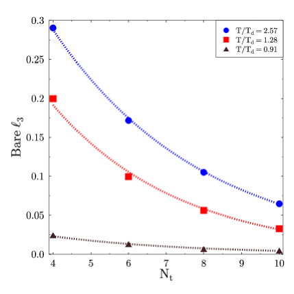
Figure 1: The bare fundamental loop as extracted from lattices with various $N_{t}$ at three different temperatures.

Renormalization of the expectation value of the bare Polyakov loop gives the exponential of a divergent mass times the length of the path [3, 4, 5, 6, 7, 8]:

$$\left|\left\langle\ell_{{\bf N}}\right\rangle\right|\sim\exp\left(-\frac{m^{div}_{N}}{T}\right)\;\;\;,\;\;\;m^{div}_{N}\;\sim\;\frac{1}{a}\;.$$ (8)

The renormalized loop, $\widetilde{\ell}_{\mathcal{R}}$, is formed by dividing the bare loop by the appropriate renormalization constant, ${\mathcal{Z}}_{\mathcal{R}}$:

$$\widetilde{\ell}_{\mathcal{R}}=\frac{1}{{\mathcal{Z}}_{\mathcal{R}}}\;\ell_{\mathcal{R}}\;\;\;,\;\;\;{\mathcal{Z}}_{\mathcal{R}}=\exp\left(-\frac{m^{div}_{\mathcal{R}}}{T}\right)\;.$$ (9)

We have developed a method to extract the divergent masses non-perturbatively [8]. The idea is to compute with a set of lattices, all at the same physical temperature, $T$, but with different values of the lattice spacing, $a$. The number of time steps, $N_{t}=1/(aT)$, varies between these lattices and the divergent mass, $am^{div}_{\mathcal{R}}$, can be extracted by comparing the different values of the bare Polyakov loops.

An alternate procedure was developed by Kaczmarek, Karsch, Petreczky, and Zantow [9] who obtain ${\mathcal{Z}}_{3}$ from the two point function of fundamental loops at short distances. Our numerical values for the triplet Polyakov loop agree approximately with their values. So far, they have not considered loops in other representations.

When the fundamental loop condenses it induces expectation values for all loops in higher representations, such as the octet and sextet loops. This can be precisely established in the limit of an infinite number of colors. Migdal and Makeenko observed that in $SU(N)$ gauge theories, expectation values factorize at large $N$ [10, 11, 12, 13, 14, 15, 16, 17]. At infinite $N$, factorization fixes the expectation value of any Polyakov loop to be equal to powers of those for the fundamental and anti-fundamental, $\widetilde{\ell}_{\overline{{\bf N}}}=(\widetilde{\ell}_{{\bf N}})^{*}$, loop [11]:

$$\left\langle\widetilde{\ell}_{\mathcal{R}}\right\rangle=\left\langle\widetilde{\ell}_{{\bf N}}\right\rangle^{p_{+}}\left\langle\widetilde{\ell}_{\overline{{\bf N}}}\right\rangle^{p_{-}}+O\left(\frac{1}{N}\right)\;\;\;.\;\;\;$$ (10)

Hence

$$\left\langle\widetilde{\ell}_{\mathcal{R}}\right\rangle=e^{ie_{\mathcal{R}}\phi}\;\left|\left\langle\widetilde{\ell}_{{\bf N}}\right\rangle\right|^{p}+O\left(\frac{1}{N}\right)\;.$$ (11)

This relation defines the $Z(N)$ charge $e_{\mathcal{R}}$ of a loop in a given representation. Thus, at infinite $N$, any renormalized loop is an order parameter for deconfinement.

To test these large $N$ relationships numerically, for each loop we define the difference between the measured loop and its value in the large $N$ limit. For three colors, the expectation value of the sextet difference loop is

$$\left\langle\delta\widetilde{\ell}_{6}\right\rangle=\left\langle\widetilde{\ell}_{6}\right\rangle-\left\langle\widetilde{\ell}_{3}\right\rangle^{2}\;,$$ (12)

and that for the octet difference loop is

$$\left\langle\delta\widetilde{\ell}_{8}\right\rangle=\left\langle\widetilde{\ell}_{8}\right\rangle-\left|\left\langle\widetilde{\ell}_{3}\right\rangle\right|^{2}\;.$$ (13)

Note that the difference loops vanish both at $T\to 0$ and at $T\to\infty$. If small, they indicate that factorization is approximately satisfied.

2 Matrix Models

Assuming that Wilson lines form the degrees of freedom in an effective theory, take as the partition function

$${\mathcal{Z}}=\int\Pi_{i}\;d{\bf L}_{{\bf N}}(i)\;\exp\left(-{\mathcal{S}}(\ell_{\mathcal{R}}(i))\right)\;.$$ (14)

Here, $i$ labels sites on a spatial lattice. The character expansion vastly reduces the possible couplings. Requiring the action to be $Z(N)$ invariant allows a sum over $Z(N)$ neutral loops:

$$N^{2}\;\Sigma_{i}\Sigma_{{\mathcal{R}}}^{e_{\mathcal{R}}=0}\;\gamma_{\mathcal{R}}\ell_{\mathcal{R}}(i)\;\,\,.$$ (15)

Add nearest neighbor interactions with couplings $\beta_{{\mathcal{R}},{\mathcal{R}}^{\prime}}$:

$${\mathcal{S}}_{\mathcal{R}}=-\frac{N^{2}}{3}\Sigma_{i,\hat{n}}\Sigma^{e_{\mathcal{R}}+e_{{\mathcal{R}}^{\prime}}=0}_{{\mathcal{R}},{\mathcal{R}}^{\prime}}\;\beta_{{\mathcal{R}},{\mathcal{R}}^{\prime}}\;{\rm Re}\;\ell_{\mathcal{R}}(i)\ell_{{\mathcal{R}}^{\prime}}(i+\hat{n})\;.$$ (16)

Kogut, Snow, and Stone showed [14] that for $N\geq 3$ in mean field approximation this model has a first order phase transition with a latent heat $\sim N^{2}$ and that

$$|\langle\widetilde{\ell}_{{\bf N}}\rangle|\approx\frac{1}{2}~{}\mbox{at}~{}T=T_{d}^{+}\;.$$ (17)

2.1 Three Color Example

The simplest $N=3$ action includes just the triplet loop:

$${\mathcal{S}}_{3}=-3\beta_{3}\;\Sigma_{i,\hat{n}}\;{\rm Re}\;\ell_{\bf 3}(i)\ell_{\bf 3}^{*}(i+\hat{n})\;\,.$$ (18)

Develop a mean field approximation by replacing all six nearest neighbors (in three space dimensions) by an average value, $\ell_{0}=\langle\ell_{\bf 3}\rangle$:

$${\mathcal{Z}}=\int\;d{\bf L}_{\bf 3}\;\exp\left(+18\beta_{3}\ell_{0}{\rm Re}\ell_{\bf 3}\right)\equiv\exp(-9{\mathcal{V}})\;\,.$$ (19)

The mean field consistency condition is

$$\ell_{0}=-\frac{1}{2\beta_{3}}\;\frac{\partial}{\partial\ell_{0}}{\mathcal{V}}\;.$$ (20)

We have studied the condensates of the four lowest representations of $SU(3)$ as a function of the coupling $\beta_{3}$ [8], which are shown in Fig. 2.

Figure 2: The condensates computed from the matrix model and compared to the lattice data[8]; for $N=3$. The lowest line is the decuplet condensate from the $N=3$ matrix model for which no lattice data is available.

Our first observation is that the ordering (fundamental, octet, sextet) agrees with that obtained from the lattice. A fit of $\langle\ell_{3}\rangle(\beta_{3})$ obtained within the matrix model to $\langle\ell_{3}\rangle(T/T_{d})$ from the lattice gives

$$\beta_{3}=(0.46\pm 0.02)+(0.33\pm 0.02)\,\frac{T}{T_{d}}\,\,.$$ (21)

Remarkably, the matrix model also predicts a sizable expectation value for the decuplet loop above $T_{d}$; so far, this has not been studied on the lattice. Also note that expectation values of $Z(3)$ neutral loops (octet and decuplet) are approximately zero in the confined phase. This is natural in a matrix model [18] but does not follow automatically in an effective theory for a scalar $\ell_{3}$ field [19, 20, 21, 22, 23].

While $\beta_{3}$ is linear in the temperature, this doesn’t seem to be true for all couplings. Fig. 3 illustrates this using the difference loops.

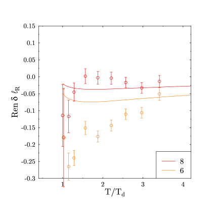
Figure 3: The difference loops computed from the matrix model and compared to the lattice data.

Clearly, the “spikes” are much smaller and broader in the matrix model than in the lattice data. From this we conclude that for a more quantitative interpretation of the lattice results more terms are needed in the matrix model.

3 Large–N Matrix Model and the Gross-Witten Point

At infinite $N$, we do not have to consider loops in higher representations as independent degrees of freedom. In mean–field approximation, we have a single–site partition function:

$${\mathcal{Z}}=\int\;d{\bf L}_{\bf N}\;\exp\left(N^{2}(2\beta\ell_{0})\;{\rm Re}\;\ell_{\bf N}\right)\equiv\exp\left(-N^{2}{\mathcal{V}}_{GW}(\beta\ell_{0})\right)\;,$$ (22)

where $\beta\equiv\beta_{N}$. The mean field condition is

$$\ell_{0}=-\frac{1}{2\beta}\;\frac{\partial}{\partial\ell_{0}}{\mathcal{V}}_{GW}(\beta\ell_{0})\;,$$ (23)

which amounts to minimizing the mean field potential

$${\mathcal{V}}_{mf}(\beta,\ell)=\beta\ell^{2}+{\mathcal{V}}_{GW}(\beta\ell)\;.$$ (24)

This has been computed in the large $N$ limit by Gross and Witten [13].

The result is nonanalytic and is given by two different potentials:

$${\mathcal{V}}_{mf}^{-}=\beta(1-\beta)\ell^{2}\;\;\;,\;\;\;\ell<\frac{1}{2\beta}\;$$ (25)

$${\mathcal{V}}_{mf}^{+}=-2\beta\ell+\beta\ell^{2}+\frac{1}{2}\log(2\beta\ell)+\frac{3}{4}\;\;\;,\;\;\;\ell>\frac{1}{2\beta}\;.$$

When $\beta<1$, the theory confines and $\ell_{0}=0$. For $\beta\geq 1$ it deconfines and

$$\ell_{0}=\frac{1}{2}\left(\;1\;+\;\sqrt{\frac{\beta-1}{\beta}}\;\;\right)\;.$$

At $\beta=1$, the potential is completely flat, i.e. it vanishes identically for $\ell\in[0,\frac{1}{2}]$.

3.1 Large–N and Mass of Polyakov Loop

The connected two point function of $\ell$ is

$$\langle\ell^{*}_{\bf N}(\vec{x})\ell_{\bf N}(0)\rangle-|\langle\ell_{\bf N}\rangle|^{2}\sim\frac{\exp(-m|\vec{x}|)}{|\vec{x}|}\;\;\;,\;\;\;|\vec{x}|\rightarrow\infty\;.$$ (26)

In the confined phase, $m=\sigma/T$, where $\sigma$ is the string tension. In the deconfined phase, one can define $m\propto m_{Debye}$.

Computing $m^{2}=\partial^{2}{\mathcal{V}}_{mf}/\partial\ell^{2}$ gives

$$m^{2}_{-}\approx 2(1-\beta)\;\;\;,\;\;\;\beta\rightarrow 1^{-}\;.$$ (27)

$$m^{2}_{+}\approx 4\sqrt{\beta-1}\;\;\;,\;\;\;\beta\rightarrow 1^{+}\;.$$ (28)

The string tension then vanishes at the transition as

$$\sigma(T)\sim(T_{d}-T)^{1/2}\;\;\;,\;\;\;T\rightarrow T_{d}^{-}\;,$$ (29)

and the Debye mass, as

$$m_{Debye}(T)\sim(T-T_{d})^{1/4}\;\;\;,\;\;\;T\rightarrow T_{d}^{+}\;.$$ (30)

Hence, at the “Gross-Witten point” [8] there is a “critical” first order transition where the order parameter jumps at $T_{d}$, yet both $m_{-}$ and $m_{+}$ vanish.

Numerical results seem to indicate that the three-color Yang-Mills theory is close to the Gross-Witten point: i) the discontinuity of the renormalized fundamental loop is approximately 1/2; ii) the “spikes” of the difference loops are of order $1/N$ near $T_{d}$ and vanish at high $T$; iii) the string tension and the Debye mass drop sharply near the transition [24].

4 Conclusions

It would be valuable to know from numerical simulations if the deconfining transition for more than three colors is close to the Gross–Witten point as well, or if that is unique to three colors. This is interesting, novel physics which can be obtained from lattice measurements at various $N$ of the renormalized Polyakov loops in hot $SU(N)$ Yang-Mills theory. Further lattice simulations with higher accuracy will also constrain the couplings of the effective matrix model description of the deconfining phase transition.
Acknowledgement: This work was done in collaboration with Yoshitaka Hatta, Kostas Orginos and Robert Pisarski. We thank the organizers of SEWM 2004 for the opportunity to attend this very productive conference.

References

- [1] G. ’t Hooft, Nucl. Phys. B 138, 1 (1978); ibid. 153, 141 (1979).
- [2] A. M. Polyakov, Phys. Lett. B 72, 477 (1978); L. Susskind, Phys. Rev. D 20, 2610 (1979).
- [3] J.-L. Gervais and A. Neveu, Nucl. Phys. B 163, 189 (1980).
- [4] A. M. Polyakov, Nucl. Phys. B 164, 171 (1980).
- [5] V. S. Dotsenko and S. N. Vergeles, Nucl. Phys. B 169, 527 (1980).
- [6] I. Y. Arefeva, Phys. Lett. B 93, 347 (1980).
- [7] U. M. Heller and F. Karsch, Nucl. Phys. B 251, 254 (1985) G. Curci, P. Menotti, G. Paffuti, Z. Phys. C 26, 549 (1985); H. Markum, M. Faber and M. Meinhart, Phys. Rev. D 36, 632 (1987); K. Enqvist, K. Kajantie, L. Karkkainen, and K. Rummukainen, Phys. Lett. B 249, 107 (1990); J. Kiskis, Phys. Rev. D 41, 3204 (1990); J. Kiskis and P. Vranas, ibid. 49, 528 (1994); C. P. Korthals Altes, Nucl. Phys. B 420, 637 (1994).
- [8] A. Dumitru, Y. Hatta, J. Lenaghan, K. Orginos and R. D. Pisarski, arXiv:hep-th/0311223.
- [9] O. Kaczmarek, F. Karsch, P. Petreczky, and F. Zantow, Phys. Lett. B 543, 41 (2002); S. Digal, S. Fortunato, and P. Petreczky, arXiv:hep-lat/0211029; O. Kaczmarek, F. Karsch, P. Petreczky and F. Zantow, Nucl. Phys. Proc. Suppl. B 129, 560 (2004); O. Kaczmarek, S. Ejiri, F. Karsch, E. Laermann and F. Zantow, arXiv:hep-lat/0312015; P. Petreczky and K. Petrov, arXiv: hep-lat/0405009.
- [10] Yu. M. Makeenko and A. A. Migdal, Phys. Lett. B 212, 221 (1980); A. A. Migdal, Phys. Rep. 102, 199 (1983).
- [11] T. Eguchi and H. Kawai, Phys. Rev. Lett. 48, 1063 (1982); with , our (10) is their (18).
- [12] A. Gocksch and F. Neri, Phys. Rev. Lett. 50, 1099 (1983); R. Narayanan and H. Neuberger, arXiv:hep-lat/0303023.
- [13] D. J. Gross and E. Witten, Phys. Rev. D 21, 446 (1980).
- [14] J. B. Kogut, M. Snow, and M. Stone, Nucl. Phys. B 200, 211 (1982).
- [15] J. Polonyi and K. Szlachanyi, Phys. Lett. B 110, 395 (1982); J. Bartholomew, D. Hochberg, P. H. Damgaard, and M. Gross, ibid. 133, 218 (1983); M. Gross and J. F. Wheater, Nucl. Phys. B 240, 253 (1984); A. Gocksch and M. Ogilvie, Phys. Rev. D 31, 877 (1985); P. H. Damgaard and A. Patkos, Phys. Lett. B 172, 369 (1986); C. X. Chen and C. DeTar, Phys. Rev. D 35, 3963 (1987); M. Ogilvie, Phys. Rev. Lett. 52, 1369 (1987).
- [16] F. Green and F. Karsch, Nucl. Phys. B 238, 297 (1984).
- [17] J. M. Drouffe and J. B. Zuber, Phys. Rep. 102, 1 (1983); S. R. Das, Rev. Mod. Phys. 59, 235 (1987); P. Di Francesco, P. H. Ginsparg and J. Zinn-Justin, Phys. Rep. 254, 1 (1995); R. C. Brower, M. Campostrini, K. Orginos, P. Rossi, C. I. Tan and E. Vicari, Phys. Rev. D 53, 3230 (1996); P. Rossi, M. Campostrini and E. Vicari, Phys. Rep. 302, 143 (1998); M. Billo, M. Caselle, A. D’Adda and S. Panzeri, Intl. Jour. Mod. Phys. A12, 1783 (1997); Yu. Makeenko, arXiv:hep-th/0001047; M. R. Douglas, I. R. Klebanov, D. Kutasov, J. Maldacena, E. Martinec and N. Seiberg, arXiv:hep-th/0307195.
- [18] A. Dumitru, J.T. Lenaghan and R.D. Pisarski: in preparation.
- [19] B. Svetitsky and L. G. Yaffe, Nucl. Phys. B 210, 423 (1982).
- [20] R. D. Pisarski, Phys. Rev. D 62, 111501 (2000).
- [21] A. Dumitru and R. D. Pisarski, Phys. Lett. B 504, 282 (2001); Phys. Lett. B 525, 95 (2002); Phys. Rev. D 66, 096003 (2002); A. Dumitru, O. Scavenius, and A. D. Jackson, Phys. Rev. Lett. 87, 182302 (2001); O. Scavenius, A. Dumitru and J. T. Lenaghan, Phys. Rev. C 66, 034903 (2002); A. Dumitru, D. Röder and J. Ruppert, arXiv:hep-ph/0311119.
- [22] P.N. Meisinger, T.R. Miller, and M.C. Ogilvie, Phys. Rev. D 65, 034009 (2002); P.N. Meisinger and M.C. Ogilvie, ibid. 65, 056013 (2002); K. Fukushima, ibid. 68, 045004 (2003); I. I. Kogan, A. Kovner and J. G. Milhano, JHEP 0212, 017 (2002).
- [23] A. Mocsy, F. Sannino and K. Tuominen, Phys. Rev. Lett. 91, 092004 (2003); JHEP 0403, 044 (2004); Phys. Rev. Lett. 92, 182302 (2004); F. Sannino and K. Tuominen, Phys. Rev. D 70, 034019 (2004).
- [24] O. Kaczmarek, F. Karsch, E. Laermann, and M. Lutgemeier, Phys. Rev. D 62, 034021 (2000).