We present a calculation of the fully differential cross section for Higgs boson production in the gluon fusion channel through next-to-next-to-leading order in perturbative QCD. We apply the method introduced in sector to compute double real emission corrections. Our calculation permits arbitrary cuts on the final state in the reaction $hh\to H+X$. It can be easily extended to include decays of the Higgs boson into observable final states. In this Letter, we discuss the most important features of the calculation, and present some examples of physical applications that illustrate the range of observables that can be studied using our result. We compute the NNLO rapidity distribution of the Higgs boson, and also calculate the NNLO rapidity distribution with a veto on jet activity.

Higgs boson production at hadron colliders: differential cross sections through next-to-next-to-leading order

With Run II of the Tevatron producing data and the LHC set to begin operation in 2007, hadron colliders will soon play a major role in understanding the mechanism of electroweak symmetry breaking. Within the Standard Model, this mechanism is linked to the Higgs boson, a scalar particle whose non-zero vacuum expectation value gives rise to the masses of all elementary particles. Finding the Higgs boson and analyzing its properties are therefore important parts of the high-energy physics program in the next decade.

Hadron colliders, while offering substantial increases in energy over existing lepton machines, present several obstacles to performing precision physics studies. Non-perturbative QCD enters the calculation of cross sections through both parton distribution functions (pdfs) of hadrons in the initial state and properties of jets in the final state. Perturbatively, the large value of the QCD coupling constant and the enhanced sensitivity to the factorization and renormalization scales force calculations of many important processes to be extended to next-to-next-to-leading order (NNLO) in the QCD coupling constant. This reduces the unphysical sensitivity of the result to the renormalization and factorization scales; also, the additional partons model the structures of both colliding hadrons and final-state jets more accurately.

There has been significant progress in the past several years in performing inclusive and semi-inclusive NNLO calculations Harlander:2002wh ; Brein:2003wg ; Harlander:2003ai ; DY ; Anastasiou:2003yy . However, because of the cuts on the final states typical for the LHC and the Tevatron, such results are of limited use. A fully differential, partonic Monte Carlo event generator is preferable. It is then guaranteed that, to a given order in the perturbative expansion, there is full control over hard emissions and the normalization of a given observable. However, this approach can not be applied if the observable is dominated by regions of the phase space where soft and collinear effects are enhanced, and the resummation of certain higher order corrections may be necessary. In such situations, shower Monte Carlo event generators are used; they correctly describe the soft and collinear limits of the real emission. However, they can not reproduce the properties of hard radiation, and are unsuitable for precision studies. Ideally, we would combine perturbative results with shower Monte Carlos to gain the advantages of both approaches. This has been achieved at NLO Frixione:2002ik , but has not been extended to higher orders. Constructing fully differential perturbative results is a first step toward this goal.

Extending exclusive calculations to higher orders is not straightforward. While at NLO this problem has been solved NLOdipole , a similar solution at NNLO is not yet available, despite significant effort NNLOdipole . The primary obstacle is the double real radiation contribution to NNLO cross sections, which contains two additional partons in the final state. The singularity structure resulting from these emissions is significantly more complex than at NLO, and prevents the use of NLO techniques.

We have recently suggested an alternative approach to the problem of real radiation at NNLO sector , which allows differential results to be obtained in an efficient, automated fashion. We have tested our idea on the realistic example of $e^{+}e^{-}\to 2~{}{\rm jets}$ at NNLO sector ; Anastasiou:2004qd . In this Letter we apply our method to calculate the fully differential cross section for Higgs boson production at hadron colliders through NNLO in QCD. Since our result retains all kinematic information, it can be used to compute arbitrary differential distributions, or to construct a partonic event generator accurate to NNLO.

The dominant production mechanism for a light Higgs boson at hadron colliders is gluon fusion, $gg\to H$, through a top quark loop. If the Higgs boson is sufficiently light, $m_{h}<2m_{t}$, its coupling to gluons can be described by a point-like vertex. Within this approximation, the NNLO corrections to the inclusive cross-section for Higgs hadroproduction have been considered recently in Harlander:2002wh , where a detailed description of the setup can be found. The two-loop virtual corrections required for Higgs production are identical for differential distributions and the total cross section. The one-loop corrections to single real-radiation processes ($gg\to H+g$, $q\bar{q}\to H+g$, $qg\to H+g$) can be computed easily with established methods Anastasiou:2003yy . The difficult contributions are the double real emission corrections that first appear at NNLO.

We use the method first presented in sector to calculate these components. We combine an expansion in plus distributions with sector decomposition decomp to separate and extract their singularities. This requires a parameterization of the phase space in which the integration region is the unit hypercube. In principle, any mapping that accomplishes this is acceptable. In practice, finding a convenient parameterization that reduces the number of sector decompositions is important for the efficiency of the approach.

For the double real emission corrections to Higgs production at NNLO, we must parameterize a $2\rightarrow 3$ particle phase space, with one massive final-state particle. We consider here $g(p_{1})+g(p_{2})\to H(h)+g(p_{3})+g(p_{4})$ as a prototypical partonic process. For a fixed energy of the partonic collision $(p_{1}+p_{2})^{2}=s$, the partonic phase space is described by four independent variables. We found it useful to employ several different parameterizations of the partonic phase space. We present here explicit formulae only for the parameterization which is the most convenient choice for the majority of diagrams. The scalar products $s_{34}=(p_{3}+p_{4})^{2}$, $s_{ih}=(p_{i}-p_{h})^{2}$, and $s_{2j}=(p_{2}-p_{j})^{2}$, where $i=1,2$ and $j=3,4$, take on simple forms in this parameterization, while the $s_{1j}$ contain overlapping singularities, and require sector decomposition when appearing in the denominator. In this parameterization, the $2\rightarrow 3$ phase space becomes

$${\rm d\Pi_{R}}=\int[dp_{3}][dp_{4}][dh]\delta^{(d)}(p_{1}+p_{2}-h-p_{3}-p_{4})$$

$$=N\int\limits_{0}^{1}{\rm d}\lambda_{1}{\rm d}\lambda_{2}{\rm d}\lambda_{3}{\rm d}\lambda_{4}\left[(1-\lambda_{1})(1-\lambda_{1}K_{m}/K_{p})\right]^{-\epsilon}$$

$$\times\left[\lambda_{1}\lambda_{2}(1-\lambda_{2})\right]^{-\epsilon}\left[\lambda_{3}(1-\lambda_{3})\right]^{1-2\epsilon}\left[\lambda_{4}(1-\lambda_{4})\right]^{-\epsilon-1/2}$$

$$\times\left[K_{p}r/(1+u)^{2}\right]^{-1+\epsilon}\left[1-\frac{\lambda_{1}K_{m}}{r(1+z)}\right],$$ (1)

where $d=4-2\epsilon$ is the space-time dimensionality, $[dq]={\rm d}q^{d-1}/(2q_{0})$, $z=m_{h}^{2}/s$, $N=\Omega(d-2)\Omega(d-3)(1-z)^{3-4\epsilon}/2^{4+2\epsilon}$, $\Omega(d)=2\pi^{d/2}/\Gamma(d/2)$, and the independent scalar products are

$$s_{1h} = -\lambda_{3}(1-z)\left[1-\lambda_{1}r(1-rt)/(r+t)\right],$$

$$s_{23} = -\lambda_{2}\lambda_{3}(1-z)\left[1+\lambda_{1}(1-rt)/r/(r+t)\right],$$

$$s_{34} = \lambda_{1}\lambda_{3}(1-\lambda_{3})(1-z)^{2}(1+u)^{2}/K_{p}/r,$$

$$s_{13} = -\frac{(1-\lambda_{3})(1-z)}{K_{p}r\left[1+\lambda_{1}(1-rt)/r/(r+t)\right]}$$ (2)

$$\times\left[A_{1}+A_{2}+2(2\lambda_{4}-1)\sqrt{A_{1}A_{2}}\right].$$

We have introduced the notations $u=(z+\lambda_{3}(1-z))/(1-\lambda_{3}(1-z)),~{}~{}r=\sqrt{u},~{}~{}~{}t=\sqrt{z},~{}~{}K_{p,m}=(r\pm t)(1\pm rt),~{}~{}A_{1}=\lambda_{1}(1-\lambda_{2})(1+u)^{2},~{}~{}A_{2}=\lambda_{2}(1-\lambda_{1})r(K_{p}-\lambda_{1}K_{m})$.

With the expressions given above, it is in principle straightforward to apply the method explained in sector to derive the finite, fully differential cross section for Higgs production at NNLO. However, some technical points warrant further discussion. A brute force application of the algorithm in sector typically produces very large expressions. It is therefore important to organize the calculation efficiently.

• We found it important to identify all possible symmetries of the process, and utilize the fact that many terms in the matrix elements are identical under a simple rotation of momentum labels, in order to reduce expression sizes.

• We found it useful to introduce a specific phase-space parameterization only for the denominators of the matrix elements. We keep the numerators written in terms of invariant masses. We therefore divide the expressions into universal denominator structures (topologies), valid for any $2\rightarrow 3$ real emission correction with one massive final-state particle, and process-dependent numerators. This allows us to implement other processes in our code very simply.

• A few topologies contain denominators that depend quadratically upon the $\lambda_{i}$. Since the full matrix elements do not contain quadratic singularities, there must be numerator structures responsible for regulating this behavior. We therefore cannot trivially keep the numerator written in terms of invariant masses for these terms. It is usually simple to identify the required numerator structure. An example found in Higgs production is the topology

  $$\frac{{\cal A}(s_{ij})}{s_{23}^{2}s_{14}^{2}}=\frac{(s_{13}s_{24}-s_{34})^{2}}{s_{23}^{2}s_{14}^{2}}\tilde{\cal A}(s_{ij}).$$ (3)

  The left-hand side of Eq.(3) naively has quadratic singularities, but, as shown, we can identify the required scalar product in the numerator that regulates these. We can now write $\tilde{\cal A}(s_{ij})$ using invariant masses, and introduce a specific parameterization for the remainder.

• As in previously studied examples sector , the matrix elements contain “line” singularities that arise when a singularity is mapped to an edge of phase space. These are removed using an additional variable change $\lambda_{i}\to\tilde{\lambda}_{i}$, as discussed in sector .

• When we convolute the partonic cross sections with the pdfs to form the hadronic cross section, the variable $z$ scales as $z\rightarrow m_{h}^{2}/(x_{1}x_{2}s_{had})$, where $s_{had}$ is the hadronic center-of-mass energy squared, and the $x_{i}$ are the fractions of the hadronic momenta carried into the hard scattering process. The partonic cross sections are distributions in $z$, and are singular in the limit $z\rightarrow 1$. Is is clear from Eq.(1) that the factor $(1-z)^{-4\epsilon}$ which regulates this limit has been extracted, and therefore singularities in $z$ and $\lambda_{i}$ can be treated identically.

After the extraction of singularities, we can combine the double real emission corrections with the remaining contributions to the hard scattering cross section. This expression is then integrated numerically together with the pdfs to form the hadronic cross section. We perform the numerical integration with the version of VEGAS described in Hahn:2004fe . We use the MRST pdf sets, with mode=1. The numerical integration we perform is 6-dimensional; this includes the four independent partonic variables and the two $x_{i}$. The CPU times required for this calculation depend strongly on both the kinematics and the requested precision. For Tevatron kinematics, reaching 1% precision on the inclusive cross section requires 0.5 hours, while obtaining 1% at the LHC requires about 1.5 hours. When constraints are imposed on the final state, the run times increase.

We have performed several checks on our calculation. We cancel $1/\epsilon$ poles numerically, as is typically done using this method sector ; Anastasiou:2004qd . The singularities begin at $1/\epsilon^{4}$, and involve all the different contributions to the final result: two-loop virtual corrections, ultraviolet renormalization, virtual corrections to NLO processes, double real emission, and collinear subtractions for pdfs; the cancellation of the singularities is therefore a strong check on the calculation. We find that the singularities cancel to a high precision for both the inclusive cross section and all distributions we have studied. For example, the $\epsilon$-expansion for the NNLO inclusive cross section at the LHC is

$$\sigma = (-0.05\pm 2)\times 10^{-6}/\epsilon^{4}+(-0.7\pm 2)\times 10^{-3}/\epsilon^{3}$$ (4)

$$+ (-0.3\pm 2)\times 10^{-3}/\epsilon^{2}+(-3\pm 9)\times 10^{-3}/\epsilon$$

$$+ (44.9\pm 0.4).$$

These results are in picobarns, and are obtained using $m_{h}=120$ GeV and $m_{t}=175$ GeV; for this and other results in this paper, higher order QCD corrections are obtained using the effective Lagrangian valid for $m_{h}<2m_{t}$ and then normalized to the exact tree-level cross section with its full $m_{t}$-dependence. The renormalization and factorization scales have been set equal to the Higgs boson mass, $\mu_{R}=\mu_{F}=m_{h}$. We have found a very good agreement between our result for the finite inclusive cross section for both Tevatron and LHC kinematics and several calculations of this quantity available in the literature Harlander:2002wh .

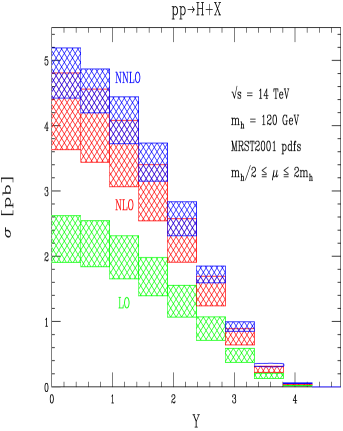
Figure 1: Bin-integrated rapidity distribution for LHC kinematics. The scale $\mu$ is varied between $m_{h}/2\leq\mu\leq 2m_{h}$. The LO, NLO, and NNLO distributions are shown.

We now present several distributions that illustrate the range of observables that can be studied using our computation. The numerical precision of all results shown is 1%. We first compute the bin-integrated rapidity distribution of the Higgs boson. We separate the entire rapidity range into twenty bins; because of the symmetry of the distribution under $Y\to-Y$, we only need to consider ten bins for $Y\geq 0$. The resulting distribution is shown in Fig.1. We have equated the renormalization and factorization scales, $\mu_{R}=\mu_{F}=\mu$, and have varied them in the range $m_{h}/2\leq\mu\leq 2m_{h}$. There are large corrections to the rapidity distribution; however, they arise primarily from the inclusive $K$-factor $K=\sigma_{\rm NNLO}/\sigma_{\rm LO}$. The rapidity dependence of the NNLO $K$-factor is small, and is insignificant if normalized to the NLO distribution. This is not unexpected; the production of the Higgs boson at the LHC is strongly dominated by the soft $z\to 1$ limit, which implies that the kinematics of the tree level process is not altered significantly by hard QCD emissions.

In Fig.2 we present the rapidity distribution with a veto on jet activity, as described in Catani:2001cr . We use the cone algorithm with $R=0.4$, and use $p_{\perp}^{veto}=40$ GeV; we therefore demand $|p_{\perp}^{j}|<40$ GeV. For this result we set $m_{h}=150$ GeV, as this cut is of particular importance for the $H\rightarrow W^{+}W^{-}$ decay channel. We show the LO, NLO, and NNLO results; we note that the LO vetoed rapidity distribution is identical to the inclusive LO rapidity distribution, as there is no additional radiation at leading order in perturbation theory. The $K$-factor is much smaller for the vetoed cross section than for the inclusive cross section; this can be easily seen by comparing the results in Fig.1 and Fig.2. One reason for this is that the average $p_{\perp}$ of the Higgs boson increases from NLO to NNLO; we find $<p_{\perp}^{\rm NLO}>=37.5$ GeV, while $<p_{\perp}^{\rm NNLO}>=44.6$ GeV. Since the additional partons recoil against the Higgs, this is equivalent to an increase in the average jet $p_{\perp}^{j}$. The increase of $p_{\perp}^{j}$ means that less of the cross section passes the veto, leading to a larger reduction in the NNLO cross-section relative to the NLO one.

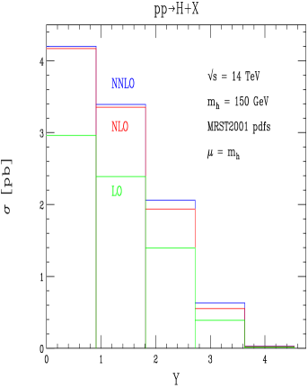
Figure 2: Bin-integrated rapidity distribution for LHC kinematics, with a jet veto of $|p_{\perp}^{j}|<40$ GeV. We have set $\mu=m_{h}$, and have included the LO, NLO, and NNLO results

.

We have described a calculation of the fully differential cross section for Higgs hadro-production at NNLO. We have utilized the method developed in sector to extract and cancel double real radiation singularities, and have extended this approach to handle processes with initial-state collinear singularities. Our result allows arbitrarily differential observables to be studied; as examples, we have presented results for the Higgs rapidity distributions at the LHC, both with and without a veto on jet activity. This approach can be easily extended to include decays of the Higgs, or can be applied to other $2\rightarrow 1$ processes of phenomenological interest. We will provide a detailed description of our calculation and present a public version of our numerical code in a forthcoming publication.

We thank T. Hahn for helpful communications regarding his numerical integration package CUBA. This work was started when the authors were visiting the Kavli Institute for Theoretical Physics, UC California, Santa Barbara. C.A. would like to thank ETH, CERN, Saclay, Fermilab and the Johns Hopkins University for their hospitality. This research was supported by the US Department of Energy under contracts DE-AC02-76SF0515, DE-FG03-94ER-40833 and the Outstanding Junior Investigator Award DE-FG03-94ER-40833, and by the National Science Foundation under contracts P420D3620414350, P420D3620434350 and partially under Grant No. PHY99-07949.

References

- (1) C. Anastasiou, K. Melnikov and F. Petriello, Phys. Rev. D 69, 076010 (2004).
- (2) R. V. Harlander and W. B. Kilgore, Phys. Rev. Lett. 88, 201801 (2002); C. Anastasiou and K. Melnikov, Nucl. Phys. B646, 220 (2002); V. Ravindran, J. Smith and W. L. van Neerven, Nucl. Phys. B665, 325 (2003).
- (3) O. Brein et al., Phys. Lett. B579, 149 (2004).
- (4) R. V. Harlander, and W. B. Kilgore, Phys. Rev. D68, 013001 (2003).
- (5) R. Hamberg et al., Nucl. Phys. B 359, 343 (1991) [Erratum-ibid. B 644, 403 (2002)].
- (6) C. Anastasiou, L. J. Dixon, K. Melnikov and F. Petriello, Phys. Rev. Lett. 91, 182002 (2003); Phys. Rev. D 69, 094008 (2004).
- (7) S. Frixione et al., JHEP 0206, 029 (2002).
- (8) R. K. Ellis et al., Nucl. Phys. B178, 421 (1981); W. T. Giele and E. W. N. Glover, Phys. Rev. D46, 1980 (1992); K. Fabricius et al., Phys. Lett. B97, 431 (1980); F. Gutbrod, G. Kramer and G. Schierholz, Z. Phys. C21, 235 (1984); Z. Kunszt and D. E. Soper, Phys. Rev. D 46, 192 (1992); S. Frixione, Z. Kunszt and A. Signer, Nucl. Phys. B 467, 399 (1996); S. Catani and M. H. Seymour, Nucl. Phys. B 485, 291 (1997) [Erratum-ibid. B 510, 503 (1997)].
- (9) J. M. Campbell and E. W. N. Glover, Nucl. Phys. B 527, 264 (1998); D. A. Kosower, Phys. Rev. D 67, 116003 (2003); S. Weinzierl, JHEP 0303, 062 (2003); A. Gehrmann-De Ridder et al., hep-ph/0403057; W. B. Kilgore, hep-ph/0403128; A. Gehrmann-De Ridder, T. Gehrmann and E. W. N. Glover, hep-ph/0407023.
- (10) C. Anastasiou, K. Melnikov and F. Petriello, Phys. Rev. Lett. 93, 032002 (2004).
- (11) T. Binoth and G. Heinrich, Nucl. Phys. B 585, 741 (2000); for earlier work see K. Hepp, Commun. Math. Phys. 2, 301 (1966); M. Roth and A. Denner, Nucl. Phys. B 479, 495 (1996).
- (12) T. Hahn, hep-ph/0404043.
- (13) S. Catani et al., JHEP 0201, 015 (2002).