Classical fields and heavy ion collisions

Abstract

This is a review of numerical applications of classical gluodynamics to heavy ion collisions. We recall some results from calculations of gluon production, discuss their implications for heavy ion phenomenology, and outline a strategy to calculate the number of quark pairs produced by these classical fields.

1 Introduction

To understand what is happening in relativistic heavy ion colliders, currently RHIC in Brookhaven and in the future the LHC at CERN, one needs to understand not only hard probes, but also bulk particle production and thermalisation. It can be argued that the large phase space densities of partons in the small-$x$ wavefunction of the nuclei generate a hard enough momentum scale to allow weak coupling methods to be used. We shall discuss first some general ideas concerning weak coupling, classical field methods in this context. Then we will go on to discuss first gluon and then quark pair production in the McLerran-Venugopalan model.

2 Relativistic heavy ion collisions

We shall be interested in studying the case where two nuclei move at the speed of light along the $x^{\pm}=0$-axes, i.e. at $\tau=0$. These nuclei then collide and leave behind them, at finite values of $\eta$ and $\tau$, some matter which is then observed in detectors located in some region, varying between different experiments, around $\eta=0$. We can divide the collision process in different stages:

1. The initial condition at $\tau=0$ depends on the properties of the nuclear wavefunction at small $x$.

2. The thermal and chemical equilibration of the matter formed at $\tau\lesssim\tau_{0}$ requires understanding of time dependent, nonequilibrium Quantum Field Theory.

3. The Quark Gluon Plasma, surviving for some fermis around $\tau_{0}\lesssim\tau\lesssim 10\textrm{fm}$. If the system reaches local thermal equilibrium, finite temperature field theory and relativistic hydrodynamics can be used to describe its behaviour.

4. Finally, for $\tau\gtrsim 10\textrm{fm}$ the system hadronises and decouples.

The question of the thermalisation timescale $\tau_{0}$ remains poorly understood. Hydrodynamical calculations have bees very successful in explaining the experimental observations, but their success depends on the assumption of a very early thermalisation time[1]. Most perturbative estimates, i.e. the bottom-up scenario[2], generically produce quite a large thermalisation time, $\tau_{0}\gtrsim 3\textrm{fm}$. On the other hand, one could argue that if the behaviour of the system is characterised by some quite large momentum scale, i.e. the saturation scale $Q_{\mathrm{s}}\sim 1\ldots 2\textrm{GeV}$, thermalisation should occur already at times $\tau_{0}\sim 1/Q_{\mathrm{s}}\sim 0.2\textrm{fm}$. It has been pointed out recently (see e.g. Ref. arnold) that plasma instabilities could provide the rapid thermalisation that hydrodynamical models require. In this context classical field models of the nuclear wavefunction and particle production can provide some insight into understanding the collision process.

3 Saturation and the classical field model

The general idea of parton saturation is that the the small-$x$ components of the nuclear wavefunction are dominated by a transverse momentum scale, the saturation scale $Q_{\mathrm{s}}$. The scale $Q_{\mathrm{s}}$ is supposed to grow for decreasing $x$ as $Q_{\mathrm{s}}^{2}(x)\sim x^{-\lambda}$ with $\lambda\approx 0.3$ giving a good fit to HERA data on deep inelastic scattering[4]. Thus for small enough $x$ or, equivalently, large enough $\sqrt{s}$ we have $Q_{\mathrm{s}}\gg\Lambda_{\textrm{QCD}}$ and we can use weak coupling methods. The presence of the scale $Q_{\mathrm{s}}$ is supposed to be caused by the color fields in the nuclear wave function becoming so strong that the gluonic interactions are dominated by the nonlinearities in the Yang-Mills Lagrangian.

This idea can also be thought of as parton percolation. Let us attach, arguing by the Heisenberg uncertainty principle, to an individual parton with transverse momentum $p_{\mathrm{T}}$ a transverse area $\sim 1/p_{\mathrm{T}}^{2}$. One expects a qualitative change in the behaviour of the system at momentum scales where the partons overlap and percolate the transverse plane: $N/p_{\mathrm{T}}^{2}\sim\pi R_{A}^{2}$, where $N$ is the number of partons and $\pi R_{A}^{2}$ the nuclear transverse area.

Because the color fields are strong, the occupation numbers of quantum states of the system are large, and it is natural ot use a classical field approximation. The saturation model has been dubbed the “Color Glass Condensate” and even called “a new form of matter”. In theory the term “color glass condensate” refers to the small-$x$ wavefunction of the nucleus, characterised by the saturation scale $Q_{\mathrm{s}}$. In practice, most applications of these ideas to heavy ion collisions have so far not been classical field computations, but perturbative calculations with some phenomenological gluon $k_{\mathrm{T}}$-distribution depending on $Q_{\mathrm{s}}^{2}(x).$

3.1 Heavy ion collisions in the classical field model

To study particle production in the classical field model we have to solve the Yang-Mills equations of motion:

$$[D_{\mu},F^{\mu\nu}]=J^{\nu},$$ (1)

with a current of two infinitely Lorentz-contracted nuclei moving along the two light cones:

$$J^{\mu}=\delta^{\mu+}\rho_{(1)}(x_{\mathrm{T}})\delta(x^{-})+\delta^{\mu-}\rho_{(2)}(x_{\mathrm{T}})\delta(x^{+}).$$ (2)

The model part of this approach comes when one must take some form for the charge density $\rho(x_{\mathrm{T}})$. The suggestion of McLerran and Venugopalan[5] was to take a random stochastic color source with a Gaussian distribution:

$$\langle\rho^{a}(x_{\mathrm{T}})\rho^{b}(y_{\mathrm{T}})\rangle=g^{2}\mu^{2}\delta^{ab}\delta^{2}(x_{\mathrm{T}}-y_{\mathrm{T}})$$ (3)

and then average all quantities calculated from $\rho(x_{\mathrm{T}})$ with this distribution. An important development has been to consider a more general $x$-dependent probability distribution $W_{x}[\rho(x_{\mathrm{T}})]$ and derive a renormalisation group equation for this distribution as a function of $x$, the JIMWLK equation[6].

3.2 Note on different saturation scales

Different ways of understanding saturation have led to different definitions of the saturation scale in the literature, which can be a source of considerable confusion.

• The $p_{\mathrm{sat}}$ in the EKRT[7] model is a final state saturation scale, not a property of the nuclear wave function (initial state), and thus conceptually a bit different from the saturation scale we have discussed so far.

• We are using the old notation of of Krasnitz et. al. In their newer work[8] they define $\Lambda_{\mathrm{s}}=g^{2}\mu$.

• By calculating the gluon distribution in the McLerran-Venugopalan model one can relate the strangth of the color source to the saturation scale $Q_{\mathrm{s}}$ defined by A. Mueller and Yu. Kovchegov (see e.g. Refs. Krasnitz:2002mn,Kovchegov:2000hz):

  $$Q_{\mathrm{s}}^{2}=\frac{g^{4}\mu^{2}C_{\mathrm{A}}}{4\pi}\ln\left(\frac{g^{4}\mu^{2}}{\Lambda_{\textrm{QCD}}^{2}}\right)$$ (4)

• The saturation scale, or radius, $Q_{\mathrm{s}}=1/R_{\mathrm{s}}$ in the work of Golec-Biernat and Wusthoff[4] or Rummukainen and Weigert[10] is the same except with $C_{\mathrm{A}}$ replaced by $C_{\mathrm{F}}$.

• For a comment on the relation to the saturation scale used by E. Iancu et. al., see Ref. Lam:2002mg.

4 Gluon production in the classical field model

The solution of the Yang-Mills equations in regions (1) and (2) is an analytically known pure gauge field[12], and gives the initial condition for the numerical solution in the forward light cone (3).

The numerical method for solving the Yang-Mills equations in the forward light cone was developed by Krasnitz, Nara and Venugopalan[13, 14]. The correct result for the transverse enegy was found in Ref. Lappi:2003bi, (see also the erratum to Ref. Krasnitz:2001qu in Ref. Krasnitz:2003jw).

The numerical computation is done in the Hamiltonian formalism. Due to the boost invariance of the initial conditions the Yang-Mills equations can be dimensionally reduced to a 2+1 dimensional gauge theory with an adjoint scalar field. With the assumption of boost invariance one is explicitly neglecting the longitudinal momenta of the gluons; a restriction that should be relaxed in future computations. In the Hamiltonian formalism one obtains directly the (transverse) energy. By decomposing the fields in Fourier modes one can also define a gluon multiplicity corresponding to the classical gauge fields.

4.1 Numerical results

Let us define the dimensionless ratios describing the energy and multiplicity:

$$f_{E}=\frac{\textrm{d}E/\textrm{d}\eta}{g^{4}\mu^{3}\pi R_{A}^{2}}\quad f_{N}=\frac{\textrm{d}N/\textrm{d}\eta}{g^{2}\mu^{2}\pi R_{A}^{2}}$$ (5)

These dimensionless ratios depend, apart from the lattice spacing $a$, only on one dimensionless parameter characterising the field strength, $g^{2}\mu R_{A}$. As can be seen from Fig. 1, for strong enough fields ($g^{2}\mu R_{A}\gtrsim 50$) both $f_{E}$ and $f_{N}$ are approximately independent of $g^{2}\mu R_{A}$ and the lattice spacing. Figure 2 shows the energy as a function of time in different field components and the spectrum of the produced gluons.

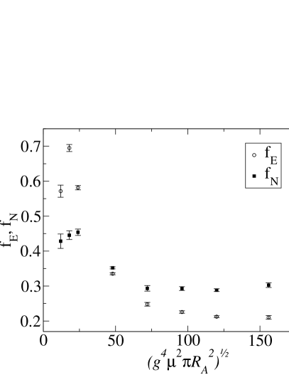
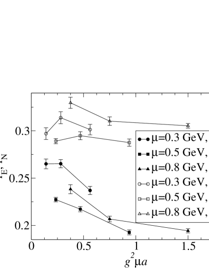
Figure 1: Left: The dependence of $f_{E}$ and $f_{N}$ on the field stregth paramater $g^{2}\mu R_{A}$. Right: The dependence of $f_{E}$ and $f_{N}$ on lattice spacing for different values of $\mu$.

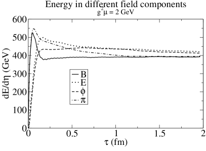
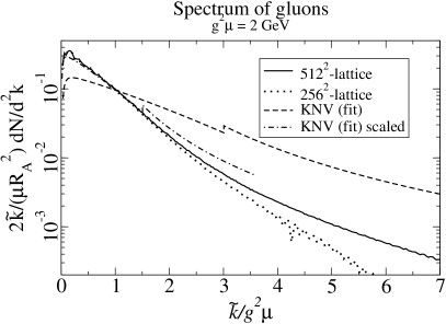
Figure 2: Left: the energy per unit rapidity is evenly distributed between different field components and almost constant after a very short time of the order of $\frac{1}{g^{2}\mu}.$ This means that the 3+1 dimensional energy density decreases as $\varepsilon\sim\tau^{-1}$ Right: The differential multiplicity for two different transverse lattice sizes. The curves labeled “KNV” are a fit to the numerical result of Ref. Krasnitz:2001qu, and KNV “scaled” after these results have been corrected (see Ref. Krasnitz:2003jw).

4.2 Phenomenology

At the level of the present discussion $g^{2}\mu$ is still a free parameter that needs to be fixed from the experimental data. One can distinguish between two broad scenarios for relating the measured results to the calculated initial state quantities.

Hydro scenario If the system thermalises fast, one can use ideal hydrodynamics to follow its subsequent evolution. In this scenario entropy and thus multiplicity are approximately conserved, but the transverse energy decreases by a factor of $\sim 3$ due to $p\textrm{d}V$-work going down the beampipe. The corresponding value for the saturation scale is $g^{2}\mu\approx 1.9\textrm{GeV}$.

Free streaming scenario Assuming that the gluons interact very weakly and do not thermalize, one can argue that longitudinal pressure is negligible and thus the transverse energy is conserved. Assuming energy conservation one gets a lower value for the saturation scale: $g^{2}\mu\sim 1.4\textrm{GeV}$. This lower value means that the multiplicity must increase during thermalisation or hadronisation of the system approximately by a factor of 2.

At least in the first case a prediction for the multiplicity at central rapidities at the LHC is straightforward; one expects to see $\left(\frac{5500\textrm{GeV}}{130\textrm{GeV}}\right)^{0.3}\times 1000\approx 3000$ particles per unit rapidity.

5 Quark pair production

Given the classical fields corresponding to gluon production a natural question to ask is: how are quark-antiquark pairs produced by these color fields? Formally quark production is suppressed by $\alpha_{\textrm{s}}$ and group theory factors compared to gluons, so in a first approximation we should be able to treat the quarks as a small perturbation and neglect their backreaction on the color fields. Heavy quark production is calculable already in perturbation theory, but one can ask how much the strong color fields change the result. Understanding light quark production would address the question of chemical equilibration; turning the color glass condensate into a quark gluon plasma.

The calculation of quark pair production, outlined in more detail in Ref. qqbartemp, proceeds by solving the Dirac equation in the background color field of the two nuclei. This can be done analytically for QED. The initial condition for $t\to-\infty$ is a negative energy plane wave. Similarly to the QED case, one can find analytically the solution for the regions $x^{\pm}>0,\ x^{\mp}<0$. These then give the initial condition at $\tau=0$ for a numerical solution of the Dirac equation in the forward light cone $\tau>0$. To find the number of quark pairs one then projects the numerically calculated wave function to a positive energy plane wave at some sufficiently large time $\tau$.

A major technical challenge in this calculation is the coordinate system. In order to include the hard sources of the color fields, the colliding nuclei, only in the initial condition of the numerical calculation, one wants to use the proper time $\tau$ instead of the Minkowski time $t$. Unlike the gluon production case, where one was able to assume strict boost invariance, one now has a nontrivial correlation between the rapidities of the quark and the antiquark. Thus, although the background gauge field is boost invariant, one must solve the Dirac equation 3+1 dimensions.

5.1 1+1-d toy model

The longitudinal direction is the one posing the most technical problems. To understand how to handle the longitudinal dimension we can construct a 1+1-dimensional toy model without the transverse dimensions. In 1+1-dimensions Dirac matrices are 2-dimensional. In the temporal gauge $A_{\tau}=0$ that we have been using throughout the calculation there is only one component, $A_{\eta},$ in the external gauge field. The mass $m^{2}_{\textrm{eff}}$ in the 1+1-dimensional model corresponds to the transverse mass $k_{\mathrm{T}}^{2}+m^{2}$ of the full theory.

The initial condition at $\tau=0$ involves a longitudinal momentum scale (the longitudinal momentum of the incoming antiquark) and thus we must use a dimensionful longitudinal variable to be able to represent the initial condition. We choose to take as our coordinates $\tau$ and $z$. The Dirac equation becomes

$$\partial_{\tau}\psi=\frac{\sqrt{\tau^{2}+z^{2}}+\gamma^{0}\gamma^{3}z}{\tau}\left(-\gamma^{0}\gamma^{3}\partial_{z}\psi-im_{\textrm{eff}}\gamma^{0}\psi\right)-i\gamma^{0}\gamma^{3}g\frac{A_{\eta}}{\tau}\psi.$$ (6)

Because of the way the coefficients depend explicitly on the coordinates the discretisation of this equation is potentially very unstable and we have to use an explicit discretisation method.

Let us take the background field as:

$$A_{\eta}=cQ_{\mathrm{s}}\tau J_{1}(Q_{\mathrm{s}}\tau).$$ (7)

For weak fields $c\ll 1$ we can compute the amplitude for quark pair production using the first order in perturbation theory (diagram (a) in Fig. 3). The result is a peak at

$$2k^{+}k^{-}=(p+q)^{2}=2m_{\textrm{eff}}^{2}\left(1+\cosh(\Delta y)\right)=Q_{\mathrm{s}}^{2}.$$ (8)

As can be seen from Fig. 4, for weak fields our numerical computation reproduces this perturbative peak. For stronger fields the numerical solution sums over all the diagrams in Fig. 3 and the position of the peak is shifted. In the full 3+1-dimensional case this peak is washed out by integration over the relative transverse momentum of the pair.

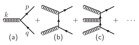
Figure 3: Diagrams contributing to the quark pair prodction amplitude in the 1+1-dimensional toy model.

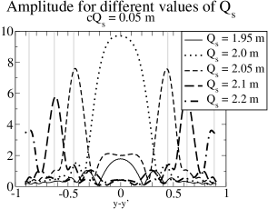
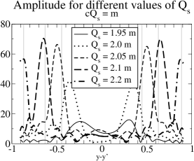
Figure 4: Absulute value of the quark pair production amplitude for different values of the oscillation scale $Q_{\mathrm{s}}$. Left: weak fields, the peaks are at the location explained by Eq. (8). Right: strong fields.

A rapid back-of-the envelope estimate suggests that with transverse lattices of the order of $256^{2}$ points (lattices from $128^{2}$ to $256^{2}$ were used in the gluon production computation) one could just manage to have a large enough lattice in the z-direction with the computers available to us. Then the computation should in principle be repeated for all the different values of $p_{\mathrm{T}}$ (of the antiquark). As this would be prohibitively expensive in terms of CPU-time one will, however, probably have to do with an interpolation from a reasonable amount of points on the $p_{\mathrm{T}}$ lattice.

6 Conclusions

Production of gluons has been computed numerically in the classical field model for heavy ion collisions, and the results are in rough agreement with RHIC observations, although not very conclusive due to the uncertainty in the numerical value of the saturation scale. A numerical calculation of the number of quark pairs produced from these classical fields is under way. It is hoped that this computation will tell us something about the how a purely gluonic system can transform into a plasma of both quarks and gluons. Understanding kinetic thermalisation in this context will require treatment of the longitudinal dimension and implementing initial conditions from the JIMWLK equation.

References

- [1] P. Kolb, These proceedings, nucl-th/0407066.
- [2] R. Baier, A. H. Mueller, D. Schiff and D. T. Son, Phys. Lett. B502, 51 (2001), [hep-ph/0009237].
- [3] P. Arnold, These proceedings, hep-ph/0409002.
- [4] K. Golec-Biernat and M. Wusthoff, Phys. Rev. D59, 014017 (1999), [hep-ph/9807513].
- [5] L. D. McLerran and R. Venugopalan, Phys. Rev. D49, 2233 (1994), [hep-ph/9309289].
- [6] H. Weigert, These proceedings.
- [7] K. J. Eskola, K. Kajantie, P. V. Ruuskanen and K. Tuominen, Nucl. Phys. B570, 379 (2000), [hep-ph/9909456].
- [8] A. Krasnitz, Y. Nara and R. Venugopalan, Nucl. Phys. A717, 268 (2003), [hep-ph/0209269].
- [9] Y. V. Kovchegov, Nucl. Phys. A692, 557 (2001), [hep-ph/0011252].
- [10] K. Rummukainen and H. Weigert, Nucl. Phys. A739, 183 (2004), [hep-ph/0309306].
- [11] C. S. Lam, G. Mahlon and W. Zhu, Phys. Rev. D66, 074005 (2002), [hep-ph/0207058].
- [12] A. Kovner, L. D. McLerran and H. Weigert, Phys. Rev. D52, 3809 (1995), [hep-ph/9505320].
- [13] A. Krasnitz and R. Venugopalan, Nucl. Phys. B557, 237 (1999), [hep-ph/9809433].
- [14] A. Krasnitz, Y. Nara and R. Venugopalan, Phys. Rev. Lett. 87, 192302 (2001), [hep-ph/0108092].
- [15] T. Lappi, Phys. Rev. C67, 054903 (2003), [hep-ph/0303076].
- [16] A. Krasnitz, Y. Nara and R. Venugopalan, Nucl. Phys. A727, 427 (2003), [hep-ph/0305112].
- [17] F. Gelis and R. Venugopalan, Phys. Rev. D69, 014019 (2004), [hep-ph/0310090].
- [18] F. Gelis, K. Kajantie and T. Lappi, hep-ph/0409058.
- [19] A. J. Baltz and L. D. McLerran, Phys. Rev. C58, 1679 (1998), [nucl-th/9804042].
- [20] A. J. Baltz, F. Gelis, L. D. McLerran and A. Peshier, Nucl. Phys. A695, 395 (2001), [nucl-th/0101024].