Effect of asymmetric strange-antistrange sea to the NuTeV anomaly

Abstract

We calculate the strange quark and antiquark distributions of the nucleon by using the effective chiral quark model, and find that the strange-antistrange asymmetry can bring a contribution of about 60–100% to the NuTeV deviation of $\sin^{2}\theta_{w}$ from the standard value measured in other electroweak processes. The results are insensitive to different inputs. The light-flavor quark asymmetry of $\overline{d}-\overline{u}$ is also investigated and found to be consistent with the experimental measurements. Therefore the chiral quark model provides a successful picture to understand the NuTeV anomaly, as well as the light-flavor quark asymmetry and the proton spin problem in previous studies.

, ,

The nucleon sea is a very active research direction of hadron physics due to its rich phenomena which are different from naive theoretical expectations and intriguing to understand strong interaction. Among various topics, the strange content of the nucleon sea is one of the most attractive issues, due to its close connection to the proton spin problem [1] and to the obscure situation about the strange-antistrange asymmetry [2]. Although much progress and achievement have been made both theoretically and experimentally, our knowledge of the strange sea is still limited. A common assumption about the strange sea is that the $s$ and $\overline{s}$ distributions are symmetric, but in fact this is established neither theoretically nor experimentally. Possible manifestations of nonperturbative effects for the strange-antistrange asymmetry have been discussed along with some phenomenological explanations [2, 3, 4, 5, 6, 7]. Also there have been some experimental analyses [8, 9, 10, 11], which suggest the $s$-$\overline{s}$ asymmetry of the nucleon sea. Therefore, the precision measurement of strange quark and antiquark distributions in the nucleon is one of the challenging and significant tasks for experimental physics.

The NuTeV Collaboration [12] reported the value of $\sin^{2}\theta_{w}$ measured in deep inelastic scattering (DIS) on nuclear target with both neutrino and antineutrino beams. Having considered and examined various source of systematic errors, the NuTeV Collaboration had the value:

$$\sin^{2}\theta_{w}=0.2277\pm 0.0013~{}(\mbox{stat})\pm 0.0009~{}(\mbox{syst}),$$

which is three standard deviations larger than the value $\sin^{2}\theta_{w}=0.2227\pm 0.0004$ measured in other electroweak processes, where $\theta_{w}$ is the Weinberg angle which is one of the important quantities in the standard model. The NuTeV Collaboration measured the value of $\sin^{2}\theta_{w}$ by using the ratio of neutrino neutral-current and charged-current cross sections on iron [12]. This procedure is closely related to the Paschos-Wolfenstein (P-W) relation [13]:

$$R^{-}=\frac{\sigma^{{\nu}N}_{NC}-\sigma^{\overline{\nu}N}_{NC}}{\sigma^{{\nu}N}_{CC}-\sigma^{\overline{\nu}N}_{CC}}=\frac{1}{2}-\sin^{2}\theta_{w},$$ (1)

which is based on the assumptions of charge symmetry, isoscalar target and $s(x)=\overline{s}(x)$. There have been a number of corrections considered for the P-W relation, for example: charge symmetry violation [14], neutron excess [15], nuclear effect [16], strange-antistrange asymmetry [17, 18], and also source for physics beyond standard model [19]. It is still obscure whether the strange-antistrange asymmetry can account for this NuTeV anomaly [20]. Cao and Signal [17] reexamined the strange-antistrange asymmetry using the meson cloud model and concluded that the second moment $S^{-}\equiv\int^{1}_{0}x[s(x)-\overline{s}(x)]\textmd{d}x$ is fairly small and unlikely to affect the NuTeV extraction of $\sin^{2}\theta_{w}$. Oppositely, Brodsky and Ma [2] proposed a light-cone meson-baryon fluctuation model to describe the $s(x)-\overline{s}(x)$ distributions and found a significantly different case from what obtained by using the meson cloud model [3, 5], as has been illustrated recently [18]. Also, Szczurek et al. [21] suggested that the effect of SU(3)_f symmetry violation may be specially important in understanding the strangeness content of the nucleon within the effective chiral quark model, and compared their results with those of the traditional meson cloud model qualitatively. In this letter, we focus our attention on the distributions of $s(x)$ and $\overline{s}(x)$, and calculate the second moment $S^{-}$ by using the effective chiral quark model. We find that the $s$-$\overline{s}$ asymmetry can remove the NuTeV anomaly by about 60–100%, and that the results are insensitive to different inputs.

The effective chiral quark model [22], which was formulated by Manohar and Georgi, is successful in explaining the Gottfried sum rule violation reported by the New Muon Collaboration [23], first done by Eichten, Hinchliffe and Quigg [24]. This model also plays an important role in explaining the proton spin problem [25] by Cheng and Li [26]. These successes naturally lead us to study the strange quark and antiquark distributions and confront them with the NuTeV result within the effective chiral quark picture. In the effective chiral quark model, the relevant degrees of freedom are constituent quarks, gluons and Goldstone (GS) bosons. It is noticeable that the effect of the internal gluon is small, when compared with those of the GS bosons and quarks, so it is negligible in this work. In this picture, the constituent quarks couple directly to the GS bosons, which are the consequences of the spontaneously broken chiral symmetry, and any low energy hadron properties should include this symmetry violation. The effective interaction Lagrangian is

$$L=\overline{\psi}(iD_{\mu}+V_{\mu})\gamma^{\mu}\psi+ig_{A}\overline{\psi}A_{\mu}\gamma^{\mu}\gamma_{5}\psi+\cdots,$$ (2)

where

$$\psi=\left(\begin{array}[]{c}u\\ d\\ s\\ \end{array}\right)$$ (3)

is the quark field and $D_{\mu}$ is the covariant derivative. The vector ($V_{\mu}$) and axial-vector ($A_{\mu}$) currents are defined in terms of GS bosons:

$$\left(\begin{array}[]{c}V_{\mu}\\ A_{\mu}\\ \end{array}\right)=\frac{1}{2}(\xi^{+}\partial_{\mu}\xi\pm\xi\partial_{\mu}\xi^{+}),$$ (4)

where $\xi=\mathrm{exp}(i\Pi/f)$ and $\Pi$ has the form:

$$\Pi\equiv\frac{1}{\sqrt{2}}\left(\begin{array}[]{ccc}\frac{\pi^{0}}{\sqrt{2}}+\frac{\eta}{\sqrt{6}}&\pi^{+}&K^{+}\\ \pi^{-}&-\frac{\pi^{0}}{\sqrt{2}}+\frac{\eta}{\sqrt{6}}&K^{0}\\ K^{-}&\overline{K^{0}}&\frac{-2\eta}{\sqrt{6}}\\ \end{array}\right).$$ (5)

Expanding $V_{\mu}$ and $A_{\mu}$ in power of $\Pi/f$ gives $V_{\mu}=0+O(\Pi/f)^{2}$ and $A_{\mu}=i\partial_{\mu}\Pi/f+O(\Pi/f)^{2}$, where the pseudoscalar decay constant is $f\simeq 93$ MeV. So the effective interaction between GS bosons and quarks becomes [24]

$$L_{\Pi q}=-\frac{g_{A}}{f}\overline{\psi}\partial_{\mu}\Pi\gamma^{\mu}\gamma_{5}\psi.$$ (6)

The framework that we use is based on timed-ordered perturbative theory in the infinite momentum frame (IMF), in which all particles are on-mass-shell so that the factorization of subprocess is automatic. We can express the quark distributions inside a nucleon as a convolution of a constituent quark distribution in a nucleon and the structure of a constituent quark. The light-front Fock decompositions of constituent quark wave functions have

$$|U\rangle = Z^{\frac{1}{2}}|u_{0}\rangle+a_{\pi}|u\pi^{0}\rangle$$ (7)

$$+\frac{a_{\pi}}{\sqrt{2}}|d\pi^{+}\rangle+a_{K}|sK^{+}\rangle+\frac{a_{\eta}}{\sqrt{6}}|u\eta\rangle,$$

$$|D\rangle = Z^{\frac{1}{2}}|d_{0}\rangle+a_{\pi}|d\pi^{0}\rangle$$ (8)

$$+\frac{a_{\pi}}{\sqrt{2}}|u\pi^{-}\rangle+a_{K}|sK^{0}\rangle+\frac{a_{\eta}}{\sqrt{6}}|d\eta\rangle,$$

where $Z$ is the renormalization constant for the bare constituent quark and $|a_{\alpha}|^{2}$ are the probabilities to find GS bosons in the dressed constituent quark states $|U\rangle$ for an $up$ quark and $|D\rangle$ for a $down$ quark. In chiral field theory, the spin-independent term is given by [27]

$$q_{j}(x)=\int^{1}_{0}\frac{\textmd{d}y}{y}P_{j\alpha/i}(y)q_{i}(\frac{x}{y}).$$ (9)

Here, $P_{j\alpha/i}(y)$ is the splitting function which gives the probability for finding a constituent quark $j$ carrying the the light-cone momentum fraction $y$ together with a spectator GS boson ($\alpha=\pi,K,\eta$), both of which coming from a parent constituent quark $i$:

$$P_{j\alpha/i}(y)=\frac{1}{8\pi^{2}}(\frac{g_{A}\overline{m}}{f})^{2}\int\textmd{d}k^{2}_{T}\frac{(m_{j}-m_{i}y)^{2}+k^{2}_{T}}{y^{2}(1-y)[m_{i}^{2}-M^{2}_{j\alpha}]^{2}},$$

where $m_{i},m_{j},m_{\alpha}$ are the masses of the $i,j$-constituent quarks and the pseudosclar meson $\alpha$, respectively,

$$M^{2}_{j\alpha}=\frac{m^{2}_{j}+k^{2}_{T}}{y}+\frac{m^{2}_{\alpha}+k^{2}_{T}}{1-y}$$ (10)

is the invariant mass squared of the final state, and $\overline{m}=(m_{i}+m_{j})/2$ is the average mass of the constituent quarks. We choose $m_{u}=m_{d}=330$ MeV, $m_{s}=480$ MeV, $m_{\pi^{\pm}}=m_{\pi^{0}}=140$ MeV and $m_{K^{+}}=m_{K^{0}}=495$ MeV. We adopt the definition of the first moment of splitting function: $\langle P_{j\alpha/i}\rangle=\int^{1}_{0}P_{j\alpha/i}(x)\textmd{d}x$ and $\langle P_{j\alpha/i}\rangle=\langle P_{\alpha j/i}\rangle\equiv\langle P_{\alpha}\rangle=|a_{\alpha}|^{2}$ [27]. It is conventional that an exponential cutoff is used in IMF calculations. Usually

$$g_{A}=g_{A}^{\prime}\textmd{exp}\bigg{[}\frac{m^{2}_{i}-M^{2}_{j\alpha}}{4\Lambda^{2}}\bigg{]},$$ (11)

with $g_{A}^{\prime}=1$ following the large $N_{c}$ argument [28], $\Lambda$ is the cutoff parameter, which is determined by the experiment data of the Gottfried sum and the constituent mass input for $\pi$, but for $K$ and $\eta$, the terms $\langle P_{K}\rangle$ and $\langle P_{\eta}\rangle$ in the Gottfried sum cancel with those in $Z=1-\frac{3}{2}\langle P_{\pi}\rangle-\langle P_{K}\rangle-\frac{1}{6}\langle P_{\eta}\rangle$:

$$S_{\mathrm{Gottfried}} = \int^{1}_{0}\frac{\mathrm{d}x}{x}[F^{p}_{2}(x)-F^{n}_{2}(x)]$$ (12)

$$= \frac{1}{3}(Z-\frac{1}{2}\left<P_{\pi}\right>+\left<P_{K}\right>+\frac{1}{6}\left<P_{\eta}\right>)$$

$$= \frac{1}{3}(1-2\left<P_{\pi}\right>).$$

Usually $\Lambda_{K}$ was given by $\Lambda_{K}=\Lambda_{\pi}=1500$ MeV [21, 27], however, the $SU_{f}(3)$ symmetry breaking requires smaller $\langle P_{K}\rangle$ and $\langle P_{\eta}\rangle$ [29], so that we should adopt a smaller value for $\Lambda_{K}$ such as from 900 MeV to 1100 MeV.

When probing the internal structure of the GS bosons, the process can be written in the following form [27]:

$$q_{k}(x)=\int\frac{\textmd{d}y_{1}}{y_{1}}\frac{\mathrm{d}y_{2}}{y_{2}}V_{k/\alpha}(\frac{x}{y_{1}})P_{\alpha j/i}(\frac{y_{1}}{y_{2}})q_{i}(y_{2}),$$ (13)

where $P_{\alpha j/i}(x)=P_{j\alpha/i}(1-x)$ and $V_{k/\alpha}(x)$ is the quark $k$ distribution function in $\alpha$ and is normalized to 1. Because the mass of $\eta$ is so high and the coefficient is so small that the fluctuation of it is suppressed, the contribution is not considered here. Assuming that the bare quark distribution functions are given in terms of the constituent quark distributions $u_{0}$ and $d_{0}$, which are normalized, we have:

$$u(x) = Zu_{0}(x)+P_{u\pi^{-}/d}\otimes d_{0}+V_{u/\pi^{+}}\otimes P_{\pi^{+}d/u}\otimes u_{0}$$

$$+ \frac{1}{2}P_{u\pi^{0}/u}\otimes u_{0}+V_{u/K^{+}}\otimes P_{K^{+}s/u}\otimes u_{0}$$

$$+ \frac{1}{4}V_{u/\pi^{0}}\otimes(P_{\pi^{0}u/u}\otimes u_{0}+P_{\pi^{0}d/d}\otimes d_{0}),$$

$$d(x) = Zd_{0}(x)+P_{d\pi^{+}/u}\otimes u_{0}+V_{d/\pi^{-}}\otimes P_{\pi^{-}u/d}\otimes d_{0}$$

$$+ \frac{1}{2}P_{d\pi^{0}/d}\otimes d_{0}+V_{d/K^{0}}\otimes P_{K^{0}s/d}\otimes d_{0}$$

$$+ \frac{1}{4}V_{d/\pi^{0}}\otimes(P_{\pi^{0}u/u}\otimes u_{0}+P_{\pi^{0}d/d}\otimes d_{0}).$$

Here, we define the notation for the convolution integral:

$$P\otimes q=\int_{x}^{1}\frac{\textmd{d}y}{y}P(y)q(\frac{x}{y}).$$ (14)

In the same way, we can have the light-flavor antiquark and strange quark and antiquark distributions:

$$\overline{u}(x) = V_{\overline{u}/\pi^{-}}\otimes P_{\pi^{-}u/d}\otimes d_{0}$$

$$+ \frac{1}{4}V_{\overline{u}/\pi^{0}}\otimes(P_{\pi^{0}u/u}\otimes u_{0}+P_{\pi^{0}d/d}\otimes d_{0}),$$

$$\overline{d}(x) = V_{\overline{d}/\pi^{+}}\otimes P_{\pi^{+}d/u}\otimes u_{0}$$

$$+ \frac{1}{4}V_{\overline{d}/\pi^{0}}\otimes(P_{\pi^{0}u/u}\otimes u_{0}+P_{\pi^{0}d/d}\otimes d_{0}),$$

$$s(x) = P_{sK^{+}/u}\otimes u_{0}+P_{sK^{0}/d}\otimes d_{0},$$

$$\overline{s}(x) = V_{\overline{s}/K^{+}}\otimes P_{K^{+}s/u}\otimes u_{0}+V_{\overline{s}/K^{0}}\otimes P_{K^{0}s/d}\otimes d_{0},~{}~{}$$

where $V_{u/\pi^{+}}=V_{\overline{d}/\pi^{+}}=V_{d/\pi^{-}}=V_{\overline{u}/\pi^{-}}=2V_{u/\pi^{0}}=2V_{\overline{u}/\pi^{0}}=2V_{d/\pi^{0}}=2V_{\overline{d}/\pi^{0}}$, $V_{\overline{s}/K^{+}}=V_{\overline{s}/K^{0}}$ and $V_{u/K^{+}}=V_{d/K^{0}}$ are taken from GRS98 parametrization of parton distributions for mesons [30]. The valence distributions $u_{v}(x)=u(x)-\overline{u}(x)$ and $d_{v}(x)=d(x)-\overline{d}(x)$ are examined to satisfy the correction normalization with the renormalization constant $Z$. From above procedure, we can calculate $S^{-}\equiv\int^{1}_{0}x[s(x)-\overline{s}(x)]\textmd{d}x$, which can bring the correction in the modified P-W relation [18]

$$R^{-}_{N}=\frac{\sigma^{\nu N}_{NC}-\sigma^{\overline{\nu}N}_{NC}}{\sigma^{\nu N}_{CC}-\sigma^{\overline{\nu}N}_{CC}}=R^{-}-\delta R^{-}_{s},$$ (15)

where $\delta R^{-}_{s}$ is the correction term to the P-W relation, which comes from the asymmetry of strangeness and reads:

$$\delta R^{-}_{s}=(1-\frac{7}{3}\sin^{2}\theta_{w})\frac{S^{-}}{Q_{v}+3S^{-}},$$ (16)

where $Q_{v}\equiv\int^{1}_{0}x[u_{v}(x)+d_{v}(x)]\textmd{d}x$. Thus what measured by NuTeV should be $\sin^{2}\theta_{w}+\delta R^{-}_{s}$, rather than $\sin^{2}\theta_{w}$ from a strict sense. One would need $\delta R^{-}_{s}\approx 0.005$ to completely explain the NuTeV deviation from the standard value of $\sin^{2}\theta_{w}$ measured in other processes.

We choose two different sets of constituent quark distributions as inputs: constituent quark (CQ) model distributions [31] and CTEQ6 parametrization [32]. The constituent quark (CQ) model distributions have the form with the initial scale $Q^{2}_{0}=0.4$ Ge$\textmd{V}^{2}$:

$$u_{0}(x) = \frac{2}{\textmd{B}[c_{1}+1,c_{1}+c_{2}+2]}x^{c_{1}}(1-x)^{c_{1}+c_{2}+1},$$

$$d_{0}(x) = \frac{1}{\textmd{B}[c_{2}+1,2c_{1}+2]}x^{c_{2}}(1-x)^{2c_{1}+1},$$ (17)

which is independent of nature of probe and its $Q^{2}$ value. Where $B[i,j]$ is the Euler beta function with $c_{1}=0.65$ and $c_{2}=0.35$ given in [31]. The other input we adopted is from CTEQ6 parametrization with $Q_{0}=1.3$ GeV:

$$u_{0}(x) = 1.7199x^{-0.4474}(1-x)^{2.9009}\cdot$$

$$\textmd{ exp}[-2.3502x](1+\textmd{exp}[1.6123]x)^{1.5917},~{}~{}$$

$$d_{0}(x) = 1.4473x^{-0.3840}(1-x)^{4.9670}\cdot$$ (18)

$$\textmd{exp}[-0.8408x](1+\textmd{ exp}[0.4031]x)^{3.0000}.~{}~{}$$

Figure 1: Distributions for $\overline{d}(x)-\overline{u}(x)$ for $\Lambda_{\pi}=1500$ MeV, the solid curve for constituent quark (CQ) model as input and the dashed curve for CTEQ6 parametrization as input within the chiral quark model. The data are from HERMES ($Q^{2}=2.3$ Ge$\textmd{V}^{2}/c^{2}$) and E866/NuSea ($Q^{2}=54$ Ge$\textmd{V}^{2}/c^{2}$) experiments [33, 34].

Table 1: The calculated results for different inputs

Parameter	$\Lambda_{K}=1100$ MeV				$\Lambda_{K}=900$ MeV
Quantity	$Z$	$Q_{v}$	$S^{-}$	$\delta R_{s}^{-}$	$\delta R_{s}^{-}$
CQ	0.731	0.846	0.00879	0.00473	0.00297
CTEQ6	0.731	0.362	0.00398	0.00498	0.00312

The calculated results of $\overline{d}(x)-\overline{u}(x)$ are shown in Fig. 1, from which we find that our results match the experiments [33, 34] well with two very different inputs of constituent quark distributions. We also get different distributions for $x\delta_{s}(x)$ in Fig. 2, from which we find that the magnitudes with CQ input are almost twice larger than those with CTEQ6 input. However, the values of $\delta R_{s}^{-}$ in Table 1 are similar and insensitive to different inputs at fixed $\Lambda_{K}$, as the uncertainties as well as $Q^{2}$ evolution of $S^{-}$ and $Q_{v}$ in the numerator and denominator of Eq. (16) can at least partially cancel each other. This means that the strange-antistrange asymmetry within the framework of the effective chiral quark model can account for about 60–100% (corresponding to $\Lambda_{K}=900$–$1100$ MeV) of the NuTeV anomaly without sensitivity to different inputs of constituent quark distributions. The adoption of a larger $\Lambda_{K}$ will bring more significant correction to the P-W relation.

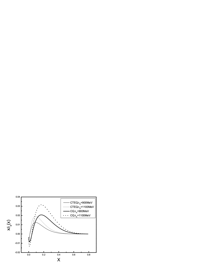
Figure 2: Distributions of $x\delta_{s}(x)$, with $\delta_{s}(x)$=$s(x)-\overline{s}(x)$ for both constituent quark (CQ) model (thick curves) and CTEQ6 parametrization (thin curves) as inputs with $\Lambda_{K}=900$ MeV (solid curves) and 1100 MeV (dashed curves ).

In summary, we calculated $\overline{d}(x)-\overline{u}(x)$ in the chiral quark model with different inputs and found that the calculated results are consistent with experiments. We also calculated $x\delta_{s}(x)$ and found that the magnitudes are sensitive to different inputs and parameters. However, the effect due to the strange-antistrange asymmetry can bring a significant contribution to the NuTeV deviation from the standard value of $\sin^{2}\theta_{w}$, of about 60–100% with reasonable parameters without sensitivity to different inputs of constituent quark distributions. Therefore the chiral quark model provides a successful picture to understand a number of anomalies concerning the nucleon sea: the light-flavor quark asymmetry [24], the proton spin problem [26], and also the NuTeV anomaly. This may imply that the NuTeV anomaly can be considered as a phenomenological support to the strange-antistrange asymmetry of the nucleon sea. Thus it is important to make a precision measurement of the distributions of $s(x)$ and $\overline{s}(x)$ in the nucleon more carefully in future experiments.

This work is partially supported by National Natural Science Foundation of China.

References

• [1] S.J. Brodsky, J. Ellis, M. Karliner, Phys. Lett. B 206 (1988) 309; J. Ellis, M. Karliner, Phys. Lett. B 213 (1988) 73; 341 (1995) 397.
• [2] S.J. Brodsky, B.-Q. Ma, Phys. Lett. B 381 (1996) 317.
• [3] A.I. Signal, A.W. Thomas, Phys. Lett. B 191 (1987) 205.
• [4] M. Burkardt, B.J. Warr, Phys. Rev. D 45 (1992) 958.
• [5] H. Holtmann, A. Szczurek, J. Speth, Nucl. Phys. A 596 (1996) 631.
• [6] H.R. Christiansen, J. Magnin, Phys. Lett. B 445 (1998) 8.
• [7] F.-G. Cao, A.I. Signal, Phys. Rev. D 60 (1999) 074021.
• [8] A.O. Bazarko $et~{}al.$, (CCFR Collab.), Z. Phys. C 65 (1995) 189.
• [9] W.G. Seligman $et~{}al.$, Phys. Rev. Lett. 79 (1997) 1213; S.A. Rabinowitz $et~{}al.$, Phys. Rev. Lett. 70 (1993) 134.
• [10] M. Arneodo $et~{}al.$, Nucl. Phys. B 483 (1997) 3.
• [11] V. Barone, C. Pascaud, F. Zomer, Eur. Phys. J. C 12 (2000) 243.
• [12] G.P. Zeller $et~{}al.$, Phys. Rev. Lett. 88 (2002) 091802.
• [13] E.A. Paschos, L. Wolfenstein, Phys. Rev. D 7 (1973) 91.
• [14] J.T. Londergan, A.W. Thomas, Phys. Lett. B 558 (2003) 132.
• [15] S. Kumano, Phys. Rev. D 66 (2002) 111301.
• [16] S. Kovalenko, I. Schmidt, J.-J. Yang, Phys. Lett. B 546 (2002) 68 (2002); S.J. Brodsky, I. Schmidt, J.-J. Yang, Phys. Rev. D 70 (2004) 116003.
• [17] F.-G. Cao, A.I. Signal, Phys. Lett. B 559 (2003) 229.
• [18] Y. Ding, B.-Q. Ma, Phys. Lett. B 590 (2004) 216.
• [19] S. Davidson $et~{}al.$, JHEP 02 (2002) 037.
• [20] S.Kretzer $et~{}al.$, Phys. Rev. Lett. 93 (2004) 041802; F.Olness $et~{}al.$, hep-ph/0312323.
• [21] A. Szczurek, A.J. Buchmann, A. Faessler, J. Phys. G: Nucl. Part. Phys. 22 (1996) 1741.
• [22] A. Manohar, H. Georgi, Nucl. Phys. B 234 (1984) 189; S.Weinberg, Physica A 96 (1979) 327.
• [23] P. Amaudruz $et~{}al.$, Phys. Rev. Lett. 66 (1991) 2712; M.Arneodo $et~{}al.$, Phys. Rev. D 50 (1994) R1.
• [24] E.J. Eichten, I. Hinchliffe, C. Quigg, Phys. Rev. D 45 (1992) 2269.
• [25] J. Ashman $et~{}al.$, Phys. Lett. B 206 (1988) 364; Nucl. Phys. B 328 (1989) 1.
• [26] T.P. Cheng, L.-F. Li, Phys. Rev. Lett. 74 (1995) 2872.
• [27] K.Suzuki, W.Weise, Nucl. Phys. A 634 (1998) 141.
• [28] S. Weinberg, Phys. Rev. Lett. 65 (1990) 1181.
• [29] X. Song, J.S. McCarthy, and H.J. Weber, Phys. Rev. D 55 (1997) 2624.
• [30] M.Glück, E. Reya, M. Stratmann, Eur. Phys. J. C 2 (1998) 159.
• [31] R.C. Hwa, M.S. Zahir, Phys. Rev. D 23 (1981) 2539; H.W. Kua, L.C. Kwek, C.H. Oh, Phys. Rev. D 59 (1999) 074025.
• [32] J. Pumplin $et~{}al.$, JHEP 0207 (2002) 012.
• [33] K. Ackerstaff $et~{}al.$, Phys. Rev. Lett. 81 (1998) 5519.
• [34] R.S. Towell $et~{}al.$, Phys. Rev. D 64 (2001) 052002.