Unification, Multiplets and Proton Decay

We make a detailed analysis of gauge coupling unification in supersymmetry. When the Standard Model gauge group is embedded in a Grand Unified Theory, new particles often appear below the GUT scale in order to predict the right phenomenology at low energy. While these new particles are beyond the reach of accelerator experiments, they change the prediction of $\alpha_{s}$. Here we classify all the $(\mathrm{SU(3)_{C},SU(2)_{L})_{U(1)_{Y}}}$ representations which improve or worsen the prediction. Running experimentally determined values of the coupling constants at two loops we calculate the allowed range of masses of fields in these representations. We explore the implication of these results in SU(5) and $\mathrm{SU}(3)^{3}$ (trinification) models. We discover that minimal trinification predicts light triplet Higgs particles which lead to proton decay with a lifetime in the vicinity of the current experimental bound.

1 Introduction

The Standard Model of particle physics provides a good description of almost all non-gravitational phenomena of known particles and their strong and electroweak interactions. Yet, its failure to address many theoretical issues has motivated a search for supersymmetry. Low energy supersymmetry is the most popular solution to the hierarchy problem. Experimentally, the best indication of supersymmetry is the prediction of gauge coupling unification in the simplest supersymmetric extension of the Standard Model (viz. MSSM). Quantitatively, the coupling constants unify in the MSSM at 99.73% confidence level, corresponding to $3\sigma$ for one degree of freedom.

From a top-down point of view, specific GUT models generically predict new particles beyond the MSSM. They change the scale dependence of the coupling constants. If all new particles are at the GUT scale or if they form complete multiplets of a unifying group, then the gauge coupling unification is as automatic as in the MSSM. However, to predict low-energy physics correctly few $(\mathrm{SU(3)_{C},SU(2)_{L})_{U(1)_{Y}}}$ multiplets usually become light. To be more explicit, let us point out a few reasons that may result in light degrees of freedom in model building

1. New particles may get masses from higher dimensional operators. In this case their mass is suppressed by $\Lambda$, the cut-off scale of the theory.

2. Often these new particles appear in the representation that contains quarks and leptons. In that case their mass may become proportional to the Yukawa couplings in the MSSM. Thus, the tiny masses of quarks and leptons in the first two generations may make these new particles lighter than the GUT scale

3. Light particles may arise as pseudo Goldstone bosons of spontaneously broken approximate global symmetries of the theory. Also, some new particles may become light in the absence of specific superpotential couplings. SUSY ensures that these couplings will not be generated by loops.

The object of this paper is to present a systematic way to talk about so called “GUT-scale threshold effects” due to these new light particles in a model-independent way. Note that there is another kind of the threshold corrections at the GUT scale because of higher dimensional operators suppressed by the Planck mass. These operators can produce significant corrections to the gauge kinetic function. For a recent discussion on effects of these operators on unification and references see [1]. In this paper we ignore these contributions of non-renormalizable operators. We demand that gauge coupling constants unify within 99.73% confidence level as in the MSSM even with new particles at intermediate mass scales. This allows us to isolate all $(\mathrm{SU(3)_{C},SU(2)_{L})_{U(1)_{Y}}}$ multiplets which, when light, push the coupling constants away from each other and worsen the prediction of $\alpha_{s}$. For example, electroweak doublets are in the category of bad particles which worsen unification when they become light. We also take the experimentally determined values of the coupling constants as input and use the constraint of unification to predict the range of masses of different representations. Constraints from unification have previously been used to estimate the mass of the colored Higgs in the SU(5) model  [2][3][4][5]. Here we present the results for all low dimensional $(\mathrm{SU(3)_{C},SU(2)_{L})_{U(1)_{Y}}}$ multiplets, irrespective of any underlying gauge symmetry in a renormalizable theory. We apply the formalism developed here to SU(5) and $\mathrm{SU}(3)^{3}$ Grand Unified Theory. In particular, we estimate the size of doublet-triplet splitting in the 5 of SU(5).

In Section 3 we perform a detail study of the $\mathrm{SU}(3)^{3}$ trinification scheme [6][7] [8][9][10][11] [12]. We construct a phenomenologically viable minimal trinification model that also preserves unification. We find that minimal trinification is not absolutely safe from proton decay constraints. In trinification specific models of Yukawa matrices predict proton decay, mediated by the scalar part of the colored Higgs, with a lifetime significantly shorter than that of SU(5) GUTs. In minimal trinification the constraint of unification lowers the mass of colored Higgs to $10^{14}\mathrm{GeV}$. We show here that in these specific models, proton decay become interesting because of smaller colored Higgs mass. We also propose here a simple extension of the minimal model, without enlarging the number of $\mathrm{SU}(3)^{3}$ multiplets, that can avoid the difficulties of minimal trinification.

2 Unification

We start by showing that gauge coupling constants unify in the MSSM with present day data and uncertainties. Next we introduce different multiplets close to the GUT scale and investigate how the constraint of exact unification can be implemented to yield new insights into the picture of unified theories.

2.1 Unification in the MSSM

We have carried out numerical calculations for the two loop RGEs of the gauge and Yukawa coupling constants from the SUSY scale $M_{S}$ to the GUT scale $M_{G}$. RGEs for both the gauge couplings and the Yukawa couplings are well documented  [13]. We take $M_{S}$ as 1 TeV and include only the Yukawa coupling of the top quark.

The prediction of unification is extremely sensitive to the used value of $\alpha_{s}(m_{Z})$ [14]. Note that there are large discrepancies in the values of the strong coupling constant determined from high energy experiments and low energy experiments (especially $\Upsilon$ decay). PDG quotes the average value as $\alpha_{s}(m_{z})=0.1187\pm 0.002$ [15]. However, the global fit to precision electroweak analysis generates a higher value ($\alpha_{s}(m_{z})=0.1213\pm 0.0018$) [16]. There are also SUSY threshold contributions from the unknown sparticle spectrum. In order to determine the sensitivity of our results to the values of $\alpha_{s}$ as well as the gaugino/squark/slepton/Higgs and Higgsino masses we performed our analysis for a series of different input parameters.

We begin with the assumption that all the sparticles other than the gauginos, appear at the scale $M_{S}$. We take winos at 200GeV and the gluinos at 700GeV. We use the following precision measurements as inputs [15]

$$\alpha_{s_{\overline{MS}}}(m_{z})=0.1187\pm 0.002,$$

$$\mathrm{sin}^{2}\theta_{w_{\overline{MS}}}(m_{z})=0.23120\pm 0.00015,$$

$$\alpha_{{em}_{\overline{MS}}}^{-1}(m_{z})=127.906\pm 0.019.$$ (1)

These quantities are given in the $\overline{MS}$ scheme. We use reference in [17] to convert them to the $\overline{DR}$ scheme, as only in the $\overline{DR}$ scheme that can we approximate the RGEs as step functions at the particle threshold  [18].

Operationally we use given values of the unified coupling constant $\alpha_{5}$ and $M_{G}$ to predict the data of Eq.(1). We find that gauge coupling constants unify with present data (using the $\chi^{2}$ fit for two degrees of freedom) at the 99.73% confidence level for all values of $\alpha_{5}$ and $M_{G}$ which lie in the ellipse shown in Fig.(1).

However, a slightly higher value of $\alpha_{s}$ improves unification significantly. If we use $\alpha_{s}(m_{z})=0.1213\pm 0.0018$ as input parameter instead, coupling constants unify at 95% confidence level.

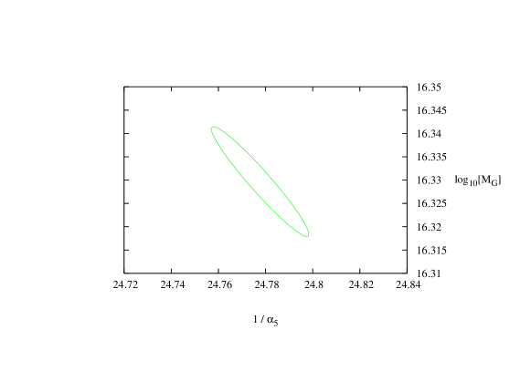
Figure 1: Plot showing 99.73% contour for two loop SUSY running with only the MSSM particle content. $\alpha_{5}$ is the unified coupling constant at the GUT scale.

Whether gauge couplings unify within error bars or not thus depends on the value of $\alpha_{s}$ one decides to use. For example, if one uses the PDG average, coupling constants do not unify within 95% confidence level. In minimal supersymmetric SU(5) model, as a result, a GUT threshold effect from the light colored Higgs is needed in order to predict $\alpha_{s}$ correctly [5]. The light colored Higgs, in turn, accelerates proton decay. Detailed discussions of proton decay in minimal SU(5) model can be found in  [2][3][4][5] [19][20]. On the other hand, if we choose the result of the global electroweak fit instead, we find that the coupling constants unify at 95% confidence level and no GUT threshold effect is needed.

To check the effects of sparticles spectrum we also perform the same calculation after introducing splittings between sleptons and squarks. Note that the overall scale for quarks and sleptons does not have significant effects in the running, because: (a) they come in complete multiplets of SU(5) and do not affect unification of couplings at 1-loop. Only squark-slepton mass splittings produce changes. (b) Squarks and sleptons have smaller contributions to the $\beta$ functions, being scalar parts of super-multiplets. We find that the contributions of a large splitting (viz. $m_{\tilde{sq}}/m_{\tilde{sl}}=(M_{3}/M_{2})^{2}$) are equivalent to shifting the input value of $\alpha_{s}$ by $1\sigma$. We also assume that the heavy Higgs scalar mass ($m_{H}$) and the Higgsino mass ($\mu$) are at $1\,$TeV. The combined threshold corrections of heavy Higgs and Higgsinos are maximum if both $m_{H}$ and $\mu$ are lighter (or heavier) than $1\,$TeV. If both $m_{H}$ and $\mu$ are assumed to be 500 GeV, we again find effects which are slightly less than the contributions of shifting the input value of $\alpha_{s}$ by $1\sigma$. To find the effect of different gaugino masses, we have also varied $M_{2}$ from 100 GeV to 600 GeV keeping $M_{3}/M_{2}$ fixed. This shift of gaugino masses also changes the prediction of $\alpha_{s}$ by $1\sigma$.

Currently, $\Upsilon$ decay measures a low value of $\alpha_{s}$ (more than $2\sigma$ smaller than the PDG average). Whereas, the global electroweak fit results in a high $\alpha_{s}$ (more than $1\sigma$ bigger than the PDG average). We also find that the fluctuation of sparticle spectrum can produce an effect, equivalent to shifting the central value of $\alpha_{s}$ by $1\sigma$. Given the sensitivity of gauge coupling unification on the input value of $\alpha_{s}$, we take a conservative and simplified approach. We choose the PDG average along with the quoted error (Eq.(1)) as input. However we present all our results at 99.73% confidence level, i.e. we basically allow $3\sigma$ variation of $\alpha_{s}$ in our calculation. Gauge coupling constants unify within 99.73% confidence level and therefore we demand that unification is maintained at this level of accuracy when contributions of new physics are added to the RGEs. We use the sparticle spectrum as was described in the beginning of this section (i.e. $M_{2}=200\,$GeV and all extra particles in the MSSM other than the gauginos, are at $1\,$TeV). Also, allowing $3\sigma$ error in the predicted value of $\alpha_{s}$ reduces the sensitivity to SUSY threshold effects.

2.2 Unification with an extra multiplet

New particles are expected to appear in various GUT models near the unification scale. If they become lighter than the unification scale, the scale dependence of the coupling constants gets modified. In this section, we discuss the effects of new multiplets in a model-independent way. However, as we already have pointed out in the introduction, we neglect contributions from higher dimensional operators.

We insert a general multiplet $(a,b)_{Y}$ along with its adjoint and give it a Dirac mass $M_{X}$. Here $a$ and $b$ are the dimensions of the representations of the multiplet under $\mathrm{SU(3)_{C}}$ and $\mathrm{SU(2)_{L}}$, and $Y$ is the hypercharge. This insertion is either going to push the coupling constants away from each other, making the unification worse compared to the case of only MSSM particle content, or it works toward having a better unification. We call all these multiplets whose insertion at a scale lower than the unification scale worsen unification prediction, “bad” multiplets, while other multiplets will be called “good” multiplets.

Now, what makes $(a,b)_{Y}$ a bad multiplet? By definition a bad multiplet worsens unification. Hence it should be clear that its insertion can never allow the central values of all the three coupling constants to coincide at a point, as they don’t even do so in the MSSM. We define the bad multiplets as the ones for which there exists no scale of insertion $M_{X}$ that produces exact unification. In order to turn this definition into a constraint on the representation $(a,b)_{Y}$ we impose the condition that the central values of the three coupling constants coincide at the unification scale. For bad multiplets this condition can never be satisfied in the acceptable region of $M_{X}<M_{G}$.

To begin, we introduce new variables for the differences of coupling constants. They are more suitable when we talk about unification

$$\Delta_{ij}(M)\equiv\frac{1}{\alpha_{i}}(M)-\frac{1}{\alpha_{j}}(M).$$ (2)

The virtue of using this alternative language may be demonstrated by inserting a 5 of SU(5). Although the coupling constants themselves change because of this insertion, $\Delta_{ij}$ remain unaltered, reflecting the fact that a 5 of SU(5) does not change unification at one loop.

To distinguish the situation before and after the insertion of the extra multiplet, the coupling constants and the difference variables found in the MSSM are denoted as $\alpha_{i}^{0}$ and $\Delta_{ij}^{0}$.

The introduction of a multiplet at scale $M_{X}$ changes the running

$$\frac{1}{\alpha_{i}}(M)=\frac{1}{\alpha_{i}^{0}}(M)-\frac{\delta\beta_{i}}{2\pi}\ln(M/M_{X}).$$ (3)

where $\alpha_{i}^{0}(M)$ is the value as determined in the MSSM at two loops and $\delta\beta_{i}$ is the contribution of the new multiplet to the corresponding $\beta$ function. Consequently, the values of $\Delta_{ij}$ are also shifted

$$\Delta_{ij}(M)=\Delta_{ij}^{0}(M)-\frac{1}{2\pi}(\delta\beta_{i}-\delta\beta_{j})\ln(M/M_{X}).$$ (4)

We impose the condition

$$\alpha_{5}=\alpha_{1}(M_{G})=\alpha_{2}(M_{G})=\alpha_{3}(M_{G}).$$ (5)

Which implies

$$\Delta_{13}(M_{G})=\Delta_{12}(M_{G})=0.$$ (6)

Eqs. (5) and (6) determine $M_{G}$. After using (4) we find that at the GUT scale

$$\Delta_{12}^{0}(M_{G}) = \frac{1}{2\pi}(\delta\beta_{1}-\delta\beta_{2})\ln(M_{G}/M_{X}),$$

$$\Delta_{13}^{0}(M_{G}) = \frac{1}{2\pi}(\delta\beta_{1}-\delta\beta_{3})\ln(M_{G}/M_{X}).$$ (7)

These equations can be solved to determine $M_{X}$ and $M_{G}$. However, we are only interested in solutions for which $M_{X}<M_{G}$. This condition along with Eq.(7) constrains the size of $\delta\beta_{i}$.

Using numerical values of $\Delta_{12}^{0}$ and $\Delta_{13}^{0}$ we find that all multiplets satisfying $\delta\beta_{2}\geq\mathrm{Max}(\delta\beta_{3},\delta\beta_{1})$ never satisfy Eq.(7). In the numerical calculation we also use an additional constraint that $10^{14}\mathrm{GeV}\leq M_{G}\leq M_{Pl}$. A detailed study reveals that all the multiplets for which the solutions to Eq.(7) satisfy our constraints can be classified as

• Type 1: $\delta\beta_{2}\geq\delta\beta_{3}$ and $\delta\beta_{1}\geq\delta\beta_{2}+\mathrm{Max}(0.2,\frac{3}{2}(\delta\beta_{2}-\delta\beta_{3}))$.

• Type 2: $\delta\beta_{2}<\delta\beta_{3}$ and $\delta\beta_{1}\geq\mathrm{Max}(0,\delta\beta_{2}-\frac{14}{11}(\delta\beta_{3}-\delta\beta_{2}))$.

By definition, both Type 1 and Type 2 are good multiplets. The factors $\frac{3}{2}(\delta\beta_{2}-\delta\beta_{3})$ in Type 1 and $\frac{14}{11}(\delta\beta_{3}-\delta\beta_{2})$ in Type 2 are included to ensure that $M_{G}>10^{14}\mathrm{GeV}$ and $M_{G}\leq 10^{19}\mathrm{GeV}$ respectively. In case of Type 1 multiplets, if $\delta\beta_{2}=\delta\beta_{1}$, we need $\delta\beta_{1}\geq\delta\beta_{2}+0.2$ so that $M_{X}$ is greater than 1TeV. For any other multiplet, there exists no acceptable set of $M_{X}$ and $M_{G}$ for which the central values of the coupling constants coincide. These are the bad multiplets.

Before proceeding let us discuss the meaning of these classifications.

1. For $\delta\beta_{2}\geq\delta\beta_{3}$, there exists a critical value of $Y$ (say $Y_{min}$). A multiplet $(a,b)_{Y}$ with $Y^{2}\geq Y_{min}^{2}$ is Type 1 and for $Y^{2}<Y_{min}^{2}$ it is a bad multiplet. $Y_{min}$ is determined by the size of $a$ and $b$. For example, in the case of the representation $(1,2)_{Y}$, we find $Y_{min}^{2}$ to be $25/24$. Thus, the multiplet $(1,2)_{1/2}$, which frequently appears in various models, is a bad multiplet.

2. Similarly, for Type 2 multiplets there are lower bounds on $\delta\beta_{1}$ implying constraints on the sizes of their hypercharge.

3. If there is a Type 1 multiplet in the theory, it lowers the GUT scale from the MSSM $M_{G}$. On the other hand, if it is a Type 2 multiplet with $\delta\beta_{2}>\delta\beta_{1}$, $M_{G}$ goes up.

4. We used the central values of the coupling constants to determine various numerical factors in the classification discussed. We use this result to identify different multiplets (which actually appear in GUT models) whether they improve or worsen unification. However dimensions of SU(3) and SU(2) representations can only have integer values and consequently the $\beta$ functions are discrete, differing by order 1 numbers. Therefore the classification is insensitive to small shifts of input values. For the same reason, constraints from the condition $M_{X}\geq 1\,$TeV are also trivially satisfied.

Table 1 lists all the low dimensional good multiplets with classifications discussed above.

$\delta\beta_{2}\geq\delta\beta_{3}$					$\delta\beta_{2}<\delta\beta_{3}$
Type 1: $Y^{2}\geq Y_{min}^{2}$					Type 2: $Y^{2}\geq Y_{min}^{2}$
SU(3)	SU(2)	$\delta\beta_{3}$	$\delta\beta_{2}$	$Y_{min}^{2}$	SU(3)	SU(2)	$\delta\beta_{3}$	$\delta\beta_{2}$	$Y_{min}^{2}$
1	1	0	0	1/6		1	1	0	0
1		0	1	25/24		1	3	0	0
		2	3	5/8		1	5	0	0
1		0	4	25/9		1	15	0	0
		3	12	255/108			10	6	25/396
		15	24	125/72			12	8	5/33
		18	32	265/144			30	10	0
1		0	10	125/24			45	40	185/198
		4	30	115/24
		20	60	25/6
		24	80	205/48

Table 1: Classification of all the low dimensional representations. Multiplet $(a,b)_{Y}$ with $\delta\beta_{2}\geq\delta\beta_{3}$ is a Type 1 good multiplet if $Y^{2}\geq Y_{min}^{2}$ and bad otherwise. Similarly, a multiplet with $\delta\beta_{2}<\delta\beta_{3}$ is a Type 2 good multiplet if its hypercharge is more than corresponding $Y_{min}$ as listed here.

At the beginning of this section, we called all multiplets, which improve unification compared to the MSSM, good multiplets. To identify them we put a stronger constraint and redefined the good multiplets as the ones for which the central values of the coupling constants coincide, with physical conditions $M_{S}\leq M_{X}<M_{G}$ and $10^{14}\mathrm{GeV}\leq M_{G}\leq M_{Pl}$. All multiplets listed in Table 1 are good multiplets based on this redefinition.

2.3 Various models

In the last section, we have identified all the small multiplets, which if appearing in the desert, worsen the degree of unification present in the MSSM. The next job is to check whether these multiplets actually appear in different GUT schemes or not. If they do, we need to make sure that there are enough light good multiplets to control the damage. To do so, we need to pick different types of theories and look at various multiplets that originate when the bigger group is decomposed to the MSSM gauge group.

We now determine which multiplets actually appear in various GUTs by decomposing the GUT multiplets into $\mathrm{SU}(3)_{\mathrm{C}}\times\mathrm{SU}(2)_{\mathrm{L}}\times\mathrm{U}(1)_{Y}$ representations. Most common GUTs have gauge groups SU(5), SO(10), $\mathrm{SU(3)}^{3}$ and $\mathrm{E}_{6}$. The MSSM is contained in SO(10) through an SU(5) and in $\mathrm{E}_{6}$ through an $\mathrm{SU(3)}^{3}$ or SO(10). Therefore we limit our attention to branching rules of SU(5) and $\mathrm{SU(3)}^{3}$. Eqs. (8) and (9) show the branching rules for the low dimensional representations of SU(5) and $\mathrm{SU(3)}^{3}$ respectively as the group is broken to $\mathrm{SU}(3)_{\mathrm{C}}\times\mathrm{SU}(2)_{\mathrm{L}}\times\mathrm{U}(1)_{Y}$ [22]. The bad multiplets are underlined in both cases.

Branching Rules for $\mathrm{SU(5)}\supset\mathrm{SU}(3)_{\mathrm{C}}\times\mathrm{SU}(2)_{\mathrm{L}}\times\mathrm{U}(1)_{Y}$.

$$5 = \underline{(1,2)_{1/2}}+(3,1)_{-1/3}$$

$$10 = (1,1)_{1}+(\bar{3},1)_{-2/3}+\underline{(3,2)_{1/6}}$$

$$15 = \underline{(1,3)_{1}}+\underline{(3,2)_{1/6}}+(6,1)_{-2/3}$$

$$24 = (1,1)_{0}+\underline{(1,3)_{0}}+(3,2)_{-5/6}+(3,2)_{5/6}+(8,1)_{0}$$

$$35 = \underline{(1,4)_{-3/2}}+\underline{(\bar{3},3)_{-2/3}}+\underline{(\bar{6},2)_{1/6}}+(\overline{10},1)_{1}$$

$$40 = (1,2)_{-3/2}+\underline{(3,2)_{1/6}}+(\bar{3},1)_{-2/3}+\underline{(\bar{3},3)_{-2/3}}+(8,1)_{1}+\underline{(\bar{6},2)_{1/6}}$$

$$45 = \underline{(1,2)_{1/2}}+(3,1)_{-1/3}+\underline{(3,3)_{-1/3}}+(\bar{3},1)_{4/3}+(\bar{3},2)_{-7/6}+(\bar{6},1)_{-1/3}+(8,2)_{1/2}$$

$$50 = (1,1)_{-2}+(3,1)_{-1/3}+(\bar{3},2)_{-7/6}+\underline{(\bar{6},3)_{-1/3}}+(6,1)_{4/3}+(8,2)_{1/2}$$ (8)

Branching Rules for $\mathrm{SU}(3)_{\mathrm{C}}\times\mathrm{SU}(3)_{\mathrm{L}}\times\mathrm{SU}(3)_{\mathrm{R}}\supset\mathrm{SU}(3)_{\mathrm{C}}\times\mathrm{SU}(2)_{\mathrm{L}}\times\mathrm{U}(1)_{Y}$

$$(3,\bar{3},1) = \underline{(3,2)_{1/6}}+(3,1)_{-1/3}$$

$$(\bar{3},1,3) = (\bar{3},1)_{1/3}+(\bar{3},1)_{1/3}+(\bar{3},1)_{-2/3}$$

$$(1,3,\bar{3}) = \underline{(1,2)_{1/2}}+\underline{(1,2)_{-1/2}}+\underline{(1,2)_{-1/2}}+(1,1)_{1}+(1,1)_{0}+(1,1)_{0}$$

$$(1,1,8) = (1,1)_{1}+(1,1)_{0}+(1,1)_{0}+(1,1)_{-1}+(1,1)_{1}+(1,1)_{0}+(1,1)_{-1}+(1,1)_{0}$$

$$(1,8,1) = \underline{(1,2)_{1/2}}+\underline{(1,2)_{-1/2}}+\underline{(1,3)_{0}}+\underline{(1,1)_{0}}$$

$$(8,1,1) = (8,1)_{0}$$ (9)

Eqs. (8) and (9) also find good multiplets, which appear in different GUT schemes. If these multiplets become lighter than the GUT scale they push the coupling constants toward each other and for some value of $M_{X}$ we predict the central values to meet exactly at a point. But a good multiplet can also worsen unification if it becomes too light. Thus we have the lower bound on the mass $(M_{X}^{min})$ above which the coupling constants unify within 99.73% confidence level. We have carried out our investigation for all low dimensional good multiplets that appear in Eqs. (8) and (9) and found the values of $(M_{X}^{min})$ from the current data. These are listed in the Table 2.

multiplets	$M_{GUT}$	$M_{X}^{min}$
$(1,1)_{1}$	$5.1\times 10^{15}-2.1\times 10^{16}$	$6.2\times 10^{12}$
$(1,1)_{-2}$	$4.8\times 10^{15}-2.1\times 10^{16}$	$9.6\times 10^{14}$
$(1,2)_{3/2}$	$2.7\times 10^{15}-2.0\times 10^{16}$	$1.9\times 10^{14}$
$(3,1)_{1/3}$	$1.5\times 10^{16}-2.2\times 10^{16}$	$1.6\times 10^{14}$
$(3,1)_{2/3}$	$1.0\times 10^{16}-2.1\times 10^{16}$	$6.9\times 10^{14}$
$(3,1)_{4/3}$	$6.6\times 10^{15}-2.1\times 10^{16}$	$2.3\times 10^{15}$
$(3,2)_{5/6}$	$2.2\times 10^{14}-1.7\times 10^{16}$	$5.6\times 10^{8}$
$(3,2)_{7/6}$	$3.7\times 10^{15}-2.0\times 10^{16}$	$8.9\times 10^{14}$
$(6,1)_{1/3}$	$1.8\times 10^{16}-2.3\times 10^{16}$	$6.5\times 10^{15}$
$(6,1)_{2/3}$	$1.4\times 10^{16}-2.2\times 10^{16}$	$6.2\times 10^{15}$
$(6,1)_{4/3}$	$8.7\times 10^{15}-2.1\times 10^{16}$	$5.9\times 10^{15}$
$(8,1)_{0}$	$5.5\times 10^{15}-2.3\times 10^{16}$	$3.0\times 10^{15}$
$(8,1)_{1}$	$1.0\times 10^{16}-2.2\times 10^{16}$	$6.5\times 10^{15}$
$(8,2)_{1/2}$	$2.5\times 10^{16}-1.7\times 10^{17}$	$4.8\times 10^{15}$
$(10,1)_{1}$	$1.3\times 10^{16}-2.2\times 10^{16}$	$1.0\times 10^{16}$

Table 2: $M_{GUT}$ and $M_{X}^{min}$ are presented for all the good multiplets in Eqs. (8) and (9). If they are heavier than $M_{X}^{min}$, the coupling constants unify within 99.73% confidence level. Note, here we have assumed that the multiplet ${\bf(8,1)_{0}}$ gets mass from self coupling.

2.4 Unification with doublets and triplets

The insertion of a full multiplet of the unifying group does not change any low energy prediction of the MSSM at one loop. However to build a phenomenologically viable model we often need to introduce mass-splittings between the elements of the full multiplet. One popular example is the famous doublet triplet splitting of a 5 of SU(5). The doublet is identified as the MSSM Higgs and we end up with an extra triplet (the colored Higgs). In fact, one extra triplet slightly lighter than $M_{G}$ improves unification.

The manifestation of this issue is more prominent in a $\mathrm{SU}(3)^{3}$ theory. The full multiplet 27 of $\mathrm{SU}(3)^{3}$, used in trinification to extract the MSSM particles as well as to break $\mathrm{SU}(3)^{3}$ to the MSSM gauge group, is the sum of three representations.

$$27=(3,\bar{3},1)+(\bar{3},1,3)+(1,3,\bar{3})$$ (10)

Usually the ${\bf(1,3,\bar{3})}$ representation is given a vev to achieve the correct breaking and this singles out ${\bf(1,3,\bar{3})}$ from the other two components of 27. Eq.(9) reveals that while ${\bf(1,3,\bar{3})}$ contains three doublets, three triplets come from ${\bf(\bar{3},1,3)}$. Hence, a mass-split between ${\bf(1,3,\bar{3})}$ and ${\bf(\bar{3},1,3)}$ is roughly equivalent to having three doublet-triplet splittings. But before embarking on details of the model we discuss unification with both doublets and triplets in the desert.

Let us introduce a doublet ${\bf(1,2)_{1/2}}$ of mass $M_{D}$ along with a triplet ${\bf(1,3)_{-1/3}}$ at a scale $M_{T}$. Using the fact that the scenario of $M_{T}=M_{D}$ is equivalent to introducing a full 5 of SU(5), the problem of two scales $M_{T}$ and $M_{D}$ can be reduced to only one effective parameter $M_{D}/M_{T}$. It is straightforward to see that, having a heavier triplet compared to the doublet is the same as the problem of a single doublet at a scale $M_{G}(\frac{M_{D}}{M_{T}})$. Alternatively, for $M_{D}>M_{T}$, the combination of a doublet and a triplet works as a single triplet of mass $M_{G}(\frac{M_{T}}{M_{D}})$. Thus, the deciding factor here is the parameter $\eta=\log_{10}(M_{D}/M_{T})$.

We scan the plane of $\eta$ and $M_{G}$ to predict the data in Eq.(1). As shown in Fig.(2), present data clearly indicate a positive value of $\eta$ within 99.73% confidence level. Note that the 99.73% ellipse in Fig.(2) do not touch the $\eta=0$ axis. It implies that the triplet needs to be slightly lighter than the GUT scale, which is in contradiction with Fig.(1). In the MSSM we have two parameters $M_{G}$ and $\alpha_{5}$. However, when an extra multiplet is added, we end up with three parameters $M_{X},M_{G}$ and $\alpha_{5}$ (in this example $M_{X}$ is replaced by $\eta$). To reduce it to two parameter plot, we determined $\alpha_{5}$ from $M_{X},M_{G}$ and the central value of $\alpha_{1}$. As a result, the ellipses shown in Fig.(2) shrink slightly.

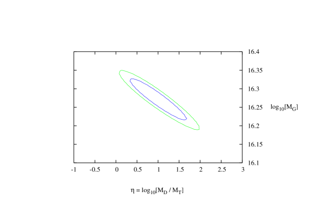
Figure 2: Plot showing 95% and 99.73% contours in the plane of $\eta$ and $M_{G}$. This clearly shows that from the viewpoint of unification a triplet lighter than a doublet is preferred.

2.5 Summary

Before ending this section, let us summarize

• We found that with MSSM particle content the gauge coupling constants unify at 99.73% confidence level.

• We have been able to identify multiplets in various GUT schemes, which if appearing within a certain range of mass scales, maintain and even improve unification. All these low dimensional good multiplets along with their preferred range of masses have been tabulated in Table 2.

• We have also been able to single out bad multiplets in different models. If they become light, these representations worsen the prediction of $\alpha_{s}$ compared to the MSSM.

• We looked carefully at the decomposition of a 27 of $\mathrm{SU}(3)^{3}$ and realized that a mass-splitting among its component representations is equivalent to a doublet-triplet splitting scenario. We found the required constraints on the mass splitting of a doublet and a triplet needed to preserve unification.

3 Constraining Trinification

In this section we discuss the trinification scheme of Grand Unification from the viewpoint established in the earlier section. We start with a short discussion of the basic idea behind trinification. Then we construct phenomenologically viable models in this scheme and check whether the constraints from unification pose any threat to these models or not.

3.1 Trinification in a nutshell

Trinification is a Grand Unified theory based on the gauge group

$$\mathrm{G}\equiv\mathrm{SU(3)_{C}\times SU(3)_{L}\times SU(3)_{R}}$$ (11)

Near the unification scale G breaks down to

$$\mathrm{G}\supset\mathrm{SU(3)_{C}\times SU(2)_{L}\times U(1)_{Y}}$$ (12)

The group G may be extended by means of a cyclic symmetry $Z_{3}$. It acts upon the three $\mathrm{SU}(3)$’s and ensures that there is only one gauge coupling constant.

The lepton, quark and the anti-quark superfields transform under G as ${\bf(1,3,\bar{3})}$, ${\bf(3,\bar{3},1)}$ and ${\bf(\bar{3},1,3)}$ respectively. Using Eq.(9) one can designate the components as

$$L^{a}\equiv(1,3,\bar{3})^{a}=\left[\begin{array}[]{ccc}l_{c}&l_{1}&l_{2}\\ e_{c}&\nu_{1}&\nu_{2}\end{array}\right]^{a};$$ (15)

$$Q^{a}\equiv(3,\bar{3},1)^{a}=\left[\begin{array}[]{cc}q&D\\ \end{array}\right]^{a};\hskip 14.22636ptQ_{c}^{a}\equiv(\bar{3},1,3)^{a}=\left[\begin{array}[]{c}u_{c}\\ d_{c_{1}}\\ d_{c_{2}}\end{array}\right]^{a}$$ (20)

where $a$ is the generation index. Let us note that every generation contains one SU(2) doublet pair and an SU(3) triplet pair in addition to the MSSM particles. This is where the small demonstration with doublet and triplet in the last section pays off. If these extra multiplets become lighter than the GUT scale, then we recover the parameter $\eta$ defined in the last section as $\log_{10}(M_{D}/M_{T})$. Only here we have three $\eta$’s, one for each generation. Combining all three of them, we redefine

$$\eta\equiv\log_{10}\big{[}M_{D^{1}}M_{D^{2}}M_{D^{3}}/M_{T^{1}}M_{T^{2}}M_{T^{3}}\big{]}$$ (21)

This parameter is going to be a useful tool in the discussion about unification in trinification. Right now we can make a very general statement that, if no other multiplets become light, present data indicates that a positive value of eta is required in order to maintain unification, as was demonstrated previously in the last section (Fig.(2)).

Usually the MSSM Higgs are obtained from a separate field $\Phi$, which has the same quantum numbers as the lepton field $L^{a}$, i.e.

$$\Phi\equiv\left[\begin{array}[]{ccc}h_{u}&h_{d_{1}}&h_{d_{2}}\\ E_{c}&N_{1}&N_{2}\end{array}\right];$$ (24)

$\Phi$ may get a nonzero vev to break the large group G. However, it alone cannot give the right breaking. One way to obtain the MSSM gauge group is to introduce another field $\Phi^{\prime}$ which transforms identically to $\Phi$ under G.

$$\langle\Phi\rangle=\langle\bar{\Phi}^{\dagger}\rangle\left[\begin{array}[]{ccc}0&0&0\\ 0&0&M\end{array}\right];\hskip 8.53581pt\langle\Phi^{\prime}\rangle=\langle\bar{\Phi^{\prime}}^{\dagger}\rangle\left[\begin{array}[]{ccc}0&0&0\\ 0&M&0\end{array}\right];\hskip 8.53581pt$$ (29)

Each vev leaves the same $\mathrm{SU}(2)_{\mathrm{L}}$ but two different $\mathrm{SU}(2)_{\mathrm{R}}$ invariant. Together they give the correct breaking. We also need to supplement the Higgs sector with its $Z_{3}$ partners.

The MSSM Yukawa couplings of leptons and quarks stem from the couplings $g_{ab}\Phi L^{a}L^{b}$ and $\lambda_{ab}\Phi Q^{a}Q_{c}^{b}$. Extra doublets and triplets get mass from the vev of $\Phi$.

$$g_{ab}\Phi L^{a}L^{b} \rightarrow g_{ab}(\langle N_{2}\rangle l_{c}^{a}l_{1}^{b}+h_{u}l_{2}^{a}\nu_{1}^{b}+h_{d_{1}}e_{c}^{a}l_{2}^{b})$$

$$\lambda_{ab}\Phi Q^{a}Q_{c}^{b} \rightarrow \lambda_{ab}(\langle N_{2}\rangle D_{c}^{a}d_{c_{2}}^{b}+h_{u}Q^{a}u_{c}^{b}+h_{d_{1}}Q^{a}d_{c_{1}}^{b})$$ (30)

There are two more parameters which show how the MSSM Higgs $H_{u}$ and $H_{d}$ are embedded in $h_{u}$ and $h_{d_{1}}$. They are determined in the potential involving $\Phi$ and $\Phi^{\prime}$. However, Eq.(30) leads to two problematic predictions irrespective of the $\Phi-\Phi^{\prime}$ potential,

$$\frac{m_{u}}{m_{d}}=\frac{m_{c}}{m_{s}}=\frac{m_{t}}{m_{b}}$$ (31)

$$\frac{M_{D^{1}}M_{D^{2}}M_{D^{3}}}{M_{T^{1}}M_{T^{2}}M_{T^{3}}}=\frac{m_{e}m_{\mu}m_{\tau}}{m_{d}m_{s}m_{b}}$$ (32)

Eq.(31) contradicts the measured quark masses and Eq.(32) does not work well with unification. Since the quarks are heavier than the charged leptons, Eq.(32) suggests that the value of $\eta$ defined in Eq.(21) is negative. But we have seen earlier that within the present data, we need a positive value of $\eta$ in order keep unification to the same order of magnitude as in the MSSM. One way to avoid these troubles might be to make both $\Phi$ and $\Phi^{\prime}$ couple to the matter superfields as well as to introduce enough mixing between $\Phi$ and $\Phi^{\prime}$ in the potential of the Higgs sector. This introduces many parameters into the calculation and prevents us from deriving an expression for $\eta$.

3.2 The Higgs Sector

$\mathrm{SU}(3)^{3}$ is broken to the MSSM gauge group in the Higgs sector. Recall that at least two multiplets $\Phi$ and $\Phi^{\prime}$ and their adjoints $\bar{\Phi}$ and $\bar{\Phi}^{\prime}$ are needed to break $\mathrm{G}\rightarrow\mathrm{SU}(3)_{\mathrm{C}}\times\mathrm{SU}(2)_{\mathrm{L}}\times\mathrm{U}(1)_{\mathrm{Y}}$. We also introduce additional singlet superfields $S$ and $S^{\prime}$. The superpotential involving S takes the form

$$W(S)=yS(\Phi\bar{\Phi}-M^{2})+hS^{2}+kS^{3}$$ (33)

It is easy to see that W(S) does have Eq.(29) as a supersymmetric vacuum with $\langle S\rangle=0$. $S^{\prime}$ has a similar potential, but it involves $\Phi^{\prime}$ instead of $\Phi$. To make this procedure $Z_{3}$ invariant we supplement $S$ with additional singlets ($S_{CL}$ and $S_{CR}$). They couple to the $Z_{3}$ counterparts of $\Phi$ ($\Phi_{CL}$ and $\Phi_{CR}$) by a potential similar to Eq.(33). Note that the superpotential of the form of Eq.(33) has another solution where only the singlet gets a nonzero vev to produce the minimum.

Construction of the rest of the Higgs potential is tricky. The MSSM Yukawa terms come from the couplings like $\Phi L^{a}L^{b}$ and $\Phi Q^{a}Q_{c}^{b}$. Hence we must find a pair of massless electroweak doublets (to be identified with the MSSM $H_{u}$ and $H_{d}$) from $\Phi$ or $\Phi^{\prime}$. All other extra multiplets should either be heavy or form complete multiplets of the GUT group if the gauge coupling unification is to be preserved.

3.2.1 First Scenario: The Minimal Model

The term minimal employed here is in the sense of minimal GUT multiplet content with interactions only at the renormalizable level. The model is built with only two Higgs multiplets which are needed to produce the right breaking.

The straightforward way is to write down all the cubic couplings involving $\Phi,\Phi^{\prime},\bar{\Phi}$ and $\bar{\Phi}^{\prime}$ (viz. $\Phi^{3},\Phi^{\prime 3}$ etc.). One can check that this results in a light doublet pair $H$ and $\bar{H}$ having the quantum numbers of $H_{d}$ and $H_{u}$ respectively. However, $\bar{H}$ resides completely inside $\bar{\Phi}$ and $\bar{\Phi}^{\prime}$, which cannot couple to $Q^{a}Q_{c}^{b}$ at the renormalizable level to produce the MSSM Yukawa couplings and fails to explain high top mass.

Clearly, not only do we need a massless electroweak doublet pair but they also need to be embedded in $\Phi$ and $\Phi^{\prime}$ to predict the correct phenomenology. This can be achieved if we forbid all cubic terms that involve $\Phi$ in the Higgs sector of the superpotential. This implies that both $h_{u}$ and $h_{d_{1}}$ inside $\Phi$ remain massless. Note that they have same quantum numbers as $H_{u}$ and $H_{d}$ respectively.

This model has been proposed earlier  [8][9] [10]. The authors have imposed a set of discrete symmetries to produce the model and shown that these symmetries can also be used to prohibit dangerous D=5 proton decay. These symmetries and their implications in trinification in detail can be found in the references.

Gauge-coupling unification in Minimal Trinification
We find that this model results in a doublet pair extra to the MSSM particle content, bad multiplets according to Eq.(9). From now on we will be referring to these extra doublets as $H_{E}$ and $\bar{H}_{E}$. Within the minimal scheme they are as light as the SUSY scale. We must find compensatory effects from extra good multiplets.

There are two sources of such effects: (a) the doublet-triplet splitting in the matter sector (i.e. $\eta$ as defined in Eq.(21)) and (b) the $Z_{3}$ partners of $\Phi$ and $\Phi^{\prime}$.

Assuming that the contributions of the light doublets $H_{E}$ and $\bar{H}_{E}$ are compensated by the doublet-triplet splitting in the matter sector, we calculated the size of the splitting ($\eta$). We find that a large positive $\eta$ ($\sim 13-14$) is necessary to produce the desired result. However, as we already have mentioned, $\eta$ is generically negative. Note that the definition of $\eta$ (Eq.(21)) involves the logarithm to the base 10. Hence large $\eta$ implies a huge mass hierarchy between the extra doublet and triplet in every generation. By suitably choosing parameters small positive $\eta$ can be generated. However, designing even $\eta\sim 4$ requires fine tuning.

Hence only if the $Z_{3}$ partners of the Higgs multiplets (i.e. $\Phi_{CL},\Phi_{CR}$) become light can unification be restored. Unlike $\Phi$, both $\Phi_{CL}$ and $\Phi_{CR}$ get masses from the singlet vev $\langle S_{CL}\rangle=\langle S_{CR}\rangle$ (equality is because of $Z_{3}$). We find that if all these multiplets ($\Phi_{CL}$, $\Phi_{CR}$, $\Phi_{CL}^{\prime}$, $\Phi_{CR}^{\prime}$) obtain masses $M_{c}\simeq(8\times 10^{13}-2\times 10^{14})\mathrm{GeV}$, the gauge couplings unify at $M_{G}\simeq 2.5\times 10^{17}\mathrm{GeV}$.

Proton decay in Minimal Trinification
The cyclic $Z_{3}$ symmetry introduces baryon number violation by operators of dimension 6. To see this, note that the full $Z_{3}$ invariant Yukawa couplings are

$$g_{ab}(\Phi L^{a}L^{b}+\Phi_{CL}Q^{a}Q^{b}+\Phi_{CR}Q^{a}_{c}Q^{b}_{c})+\lambda_{ab}(\Phi Q^{a}Q_{c}^{b}+\Phi_{CL}Q^{a}_{c}L^{b}+\Phi_{CR}L^{a}Q^{b})$$ (34)

$\Phi_{CL}$ and $\Phi_{CR}$ contain triplets (Eq.(9)) and the scalar components of these fields can mediate proton decay via D=6 operators. Note that the coupling $\Phi L^{a}L^{b}$ gives leptons their masses and $\Phi_{CL}Q^{a}Q^{b}$ produces a quark-quark-Higgs triplet vertex. Because of $Z_{3}$, these two different operators have the same coupling constant. Similarly, the strength of the lepton-quark-Higgs triplet vertex (from the operator $\Phi_{CL}Q^{a}_{c}L^{b}$) and the quark masses (from the operator $\Phi Q^{a}Q_{c}^{b}$) are related. As an example, we estimate of proton lifetime from $p\rightarrow K^{+}\bar{\nu}$

$$\Gamma(p\rightarrow K^{+}\bar{\nu})=\frac{1}{\tau_{p}}\sim\frac{g_{11}^{2}\lambda_{22}^{2}}{16\pi^{2}}\frac{m_{p}^{5}}{M_{c}^{4}}$$ (35)

$M_{c}\sim 10^{14}\mathrm{GeV}$ and the values of the coupling constants depend on the exact structure of Yukawa matrices. A naive estimation would be $\lambda_{22}\sim\frac{\surd{2}m_{c}}{v_{u}}$ and $g_{11}\sim\frac{\surd{2}m_{e}}{v_{d}}$. For $\tan\beta=10$, we find that $\tau_{p}\sim 10^{39}$ years. This estimation seems to be quite safe from recent results from Super-Kamiokande ($\tau_{p}\geq 2.3\times 10^{33}$ years)  [23]. However, a detailed study of models of Yukawa matrices reveals that proton lifetime can be far lower than $10^{39}$ years. To support this claim we give examples of few models where the lifetime may substantially be brought down.

• We oversimplified when we estimated $\lambda_{22}$ and $g_{11}$. Leptons get mass from the couplings $g_{ab}\Phi L^{a}L^{b}$ and $g^{\prime}_{ab}\Phi^{\prime}L^{a}L^{b}$. Now imagine that the MSSM Higgs $H_{d}$ is mostly contained in $\Phi^{\prime}$ but the elements in the first generation of $g$ is much bigger than that of $g^{\prime}$ so that electron mass is mostly coming from the coupling $g_{ab}\Phi L^{a}L^{b}$. In that case, $g_{11}$ can be as big as 1. Thus bringing down the proton lifetime to $10^{30}$ years.

• More subtle examples come from the understanding that flavor basis for quarks and leptons are not related in trinification. Quark and lepton masses are related to the matrices $\lambda$ and $g$ respectively. To simplify the scenario, let us assume that both of them are diagonalized in the same basis. However, they do not need to have same pattern of hierarchy in the matrix elements. In particular, if $\lambda$ and $g$ have inverted hierarchies with respect to each other, then the first generation of quarks (lightest) are related to the third generation of leptons (heaviest). In that case proton decay is accelerated and following the crude method of estimations, we used earlier, we find $\tau_{p}\sim 10^{32}$ years.

The proton lifetime in trinification is model dependent. In minimal trinification the Higgs triplets are predicted to be light. We find that there are specific models in which protons are predicted to decay with an observable lifetime. The additional pair of Higgs doublets may also produce large FCNC effects, suppressed by its mass. Turning these arguments around, we can use the experimental bounds on proton decay as well as on FCNC as model building constraints while designing the Yukawa matrices in minimal trinification.

How to avoid troublesome extra light doublets ?
We must extend the model beyond the minimal scheme. This can be achieved in two ways. In the next scenario we will keep the particle content minimal, but introduce higher dimensional operators, which make all extra multiplets heavy. Lastly, we will show another approach where new multiplets will be added to the Higgs sector.

3.2.2 Second Scenario: The Minimal Model + New Operators

In the last scenario, we found that we need to forbid the trilinear couplings ($\Phi^{3},\Phi^{2}\Phi^{\prime}$ etc.) in order to generate a high top mass. On the other hand, this results in an extra massless electroweak doublet pair.

To give masses to this doublet pair we introduce higher dimensional operators that involve $\Phi$ and $\Phi^{\prime}$. No trilinear coupling involving $\Phi$ is employed. Following is one example of such a potential.

$$W(\Phi,\Phi^{\prime}) = gS_{1}(\Phi\bar{\Phi}-M^{2})+g^{\prime}S^{\prime}_{1}(\Phi^{\prime}\bar{\Phi}^{\prime}-M^{2})+\alpha\Phi^{\prime 3}+\beta\bar{\Phi}\bar{\Phi}^{\prime 3}$$ (36)

$$+\frac{\gamma_{1}}{\Lambda}(\Phi^{\prime}\bar{\Phi}\Phi\bar{\Phi}^{\prime})+\frac{\gamma_{2}}{\Lambda}(\Phi\bar{\Phi}\Phi^{\prime}\bar{\Phi})+\frac{\gamma_{3}}{\Lambda}(\Phi^{\prime}\bar{\Phi}^{\prime}\Phi^{\prime}\bar{\Phi})$$

This potential keeps two combinations of $h_{d_{1}},h_{d_{2}}$ and $h_{d_{1}}^{\prime}$, as well as one combination of $\bar{h}_{d_{2}}$ and $\bar{h}_{d_{1}}^{\prime}$ massless along with $h_{u}$. All other doublets become heavy. We recover the MSSM Higgs as $h_{u}$ and one combination of $h_{d_{1}},h_{d_{2}}$ and $h_{d_{1}}^{\prime}$. The other two degrees of freedom are being eaten by the gauge superfields. A similar mechanism follows for the fields with quantum numbers ${\bf(1,1)_{\pm 1}}$. While $E_{c}^{\prime}$ and $\bar{E}_{c}$ get mass from the potential, $E,\bar{E}^{\prime}$ remain light and are eaten fields.

Not only are the MSSM Higgs fields obtained from $\Phi$ and $\Phi^{\prime}$, there is enough mixing to avoid Eq.(31). Relying on higher-dimensional operators, though, results in one doublet being slightly light. If the cut-off scale $\Lambda$ is assumed to be $M_{Pl}$, we end up with a doublet of mass $\sim 10^{14}$GeV. However this effect is easily compensated if we make $Z_{3}$ partners of $\Phi$ and $\Phi^{\prime}$ slightly light. Note, for $M_{C}\sim 10^{16}$ years proton becomes extremely stable.

3.2.3 Third Scenario: The Minimal Model + New Multiplets

An alternative approach is to enrich the Higgs sector by adding new multiplets. Trinification models with one extra multiplet  [10] and with several different multiplets  [7][24] have been proposed earlier. For completeness we mention here how the problem of the minimal model may be resolved by adding one extra Higgs superfield pair $\Phi^{\prime\prime}-\bar{\Phi}^{\prime\prime}$ with its $Z_{3}$ conjugates. None of the new multiplets have vevs. $\Phi^{\prime\prime},\bar{\Phi}^{\prime\prime}$ are given a mass term $M\Phi^{\prime\prime}\bar{\Phi}^{\prime\prime}$ as well as a mixing with $\bar{\Phi},\bar{\Phi}^{\prime}$ by $f\bar{\Phi}\bar{\Phi}^{\prime}\bar{\Phi}^{\prime\prime}$. This rotates the doublet ${\bf(1,2)_{+1/2}}$ from $\bar{\Phi}$ and $\bar{\Phi}^{\prime}$ to $\Phi^{\prime\prime}$. We also need additional Yukawa couplings $g_{ab}^{\prime\prime}\Phi^{\prime\prime}L^{a}L^{b}$ and $\lambda_{ab}^{\prime\prime}\Phi^{\prime\prime}Q^{a}Q_{c}^{b}$ to give masses to up-type quarks. All extra particles in the Higgs sector are at the GUT scale. Thus proton decay is delayed beyond the reach of experiments. We also have a doublet and a triplet in the matter sector in each generation that may remain light, as their masses are related to the Yukawa couplings. However, for $\eta\sim 0$ each doublet-triplet pair forms a 5 of SU(5) and do not change any low energy prediction at one loop.

4 Conclusion

$\mathrm{SU}(3)^{3}$ gives an alternative scenario of Grand Unification. There are also some indications from string theory that MSSM may be embedded in a $\mathrm{SU}(3)^{3}$ based group  [25]. Further, trinification is probably the safest GUT as far as proton decay is concerned.

We started out this paper with the issue of the effects of intermediate mass scales on gauge coupling unification. We predicted masses of different particles. We investigated trinification with these results. We constructed the minimal model and found that it produces the right phenomenology. However, the constraint of unification predicts light colored Higgs which resulted in important proton decay with an experimentally accessible lifetime. We also proposed a simple extension with minimal particle content but with higher dimensional operators. It produces the right phenomenology and keeps unification automatic with proton decay delayed beyond the reach of next generation experiments.

References

- [1] K. Tobe and J. D. Wells, Phys. Lett. B 588, 99 (2004) [arXiv:hep-ph/0312159].
- [2] J. Hisano, H. Murayama and T. Yanagida, Phys. Rev. Lett. 69, 1014 (1992).
- [3] J. Hisano, T. Moroi, K. Tobe and T. Yanagida, Mod. Phys. Lett. A 10, 2267 (1995) [arXiv:hep-ph/9411298].
- [4] J. Hisano, Y. Nomura and T. Yanagida, Prog. Theor. Phys. 98, 1385 (1997) [arXiv:hep-ph/9710279].
- [5] H. Murayama and A. Pierce, Phys. Rev. D 65, 055009 (2002) [arXiv:hep-ph/0108104].
- [6] S. L. Glashow, Print-84-0577 (BOSTON)
- [7] G. Lazarides and C. Panagiotakopoulos, Phys. Lett. B 336, 190 (1994) [arXiv:hep-ph/9403317].
- [8] G. R. Dvali and Q. Shafi, Phys. Lett. B 326, 258 (1994) [arXiv:hep-ph/9401337].
- [9] G. R. Dvali and Q. Shafi, Phys. Lett. B 339, 241 (1994) [arXiv:hep-ph/9404334].
- [10] G. R. Dvali and Q. Shafi, Prepared for ICTP Summer School in High-energy Physics and Cosmology, Trieste, Italy, 10 Jun - 26 Jul 1996
- [11] S. Willenbrock, Phys. Lett. B 561, 130 (2003) [arXiv:hep-ph/0302168].
- [12] J. E. Kim, Phys. Lett. B 591, 119 (2004) [arXiv:hep-ph/0403196].
- [13] V. D. Barger, M. S. Berger and P. Ohmann, Phys. Rev. D 47, 1093 (1993) [arXiv:hep-ph/9209232].
- [14] I. Dorsner, Phys. Rev. D 69, 056003 (2004) [arXiv:hep-ph/0310175].
- [15] S. Eidelman et al. [Particle Data Group Collaboration], Phys. Lett. B 592, 1 (2004).
- [16] J. Erler and P. Langacker, “ Electroweak model and constraints on new physics,” Phys. Lett. B 592, 1 (2004).
- [17] S. P. Martin and M. T. Vaughn, Phys. Lett. B 318, 331 (1993) [arXiv:hep-ph/9308222].
- [18] I. Antoniadis, C. Kounnas and K. Tamvakis, Phys. Lett. B 119, 377 (1982).
- [19] B. Bajc, P. F. Perez and G. Senjanovic, Phys. Rev. D 66, 075005 (2002) [arXiv:hep-ph/0204311].
- [20] B. Bajc, P. F. Perez and G. Senjanovic, arXiv:hep-ph/0210374.
- [21] W. de Boer and C. Sander, Phys. Lett. B 585, 276 (2004) [arXiv:hep-ph/0307049].
- [22] R. Slansky, Phys. Rept. 79, 1 (1981).
- [23] K.Kobayashi, Talk given at SUSY 04.
- [24] G. Lazarides and C. Panagiotakopoulos, Phys. Rev. D 51, 2486 (1995) [arXiv:hep-ph/9407286].
- [25] J. E. Kim, arXiv:hep-ph/0310158.