SATURATION SCALE FROM THE BALITSKY–KOVCHEGOV EQUATION

Abstract

Recently Munier and Peschanski presented an analysis of the Balitsky–Kovchegov (BK) equation concerning the extraction of the saturation scale, using a simpler equation. We numerically analyze the full BK equation confirming the universality of their analysis.

1 Introduction

The Balitsky–Kovchegov equation [1, 2] describes saturation [3] in gamma – nucleus deep inelastic scattering, when the structure function $F_{2}\sim\log(1/x_{B})$ for the Bjorken variable $x_{B}\to 0$. To be more precise, this behaviour appears in the region where the photon virtuality $Q^{2}<Q_{s}^{2}(x_{B})$. Here $Q_{s}^{2}$ is the saturation scale which rises with decreasing $x_{B}$. Thus the famous BFKL growth [4] in the region $Q^{2}>Q_{s}^{2}(x_{B})$, where $F_{2}\sim x_{B}^{-\lambda}$, is tamed due to saturation effects generated by the BK equation. The emergence of the saturation scale and its energy dependence is the key issue in analyses of saturation. Recently, a very elegant method of the extraction of the saturation scale was developed in [5], based on a simplified version of the BK equation. According to mathematical properties of this equation, the obtained results are universal and concern also the full BK equation. In this presentation we show numerical results which support this claim.

2 Munier–Peschanski analysis

In the space of transverse gluon momentum $k$, the BK equation reads

$$\partial_{Y}\phi=\overline{\alpha}_{s}\chi(-\partial_{L})\phi-\overline{\alpha}_{s}\phi^{2}\,,$$ (1)

where $\phi(Y,L)$ is the Fourier transform of the quark dipole–nucleon scattering amplitude [2]. Here $\chi(\gamma)=2\psi(1)-\psi(\gamma)-\psi(1-\gamma)$ is the BFKL characteristic function [4], rapidity $Y=\ln(1/x_{B})$, and $L=\ln(k^{2}/k_{0}^{2})$. The structure function $F_{2}$ at small $x_{B}$ can be computed from solutions of the BK equation .

Eq. (1) is nonlinear, with the linear part given by the BFKL function. The nonlinearity is responsible for saturation, taming the BFKL growth generated by the linear part alone. In [5] a remarkable simplification was done approximating the linear part by the Taylor expansion $\chi(\gamma)\simeq\chi_{c}+\chi_{c}^{\prime}(\gamma-\gamma_{c})+\textstyle{1\over 2}\chi_{c}^{\prime\prime}(\gamma-\gamma_{c})^{2}$, where $\gamma_{c}\simeq 0.63$ obeys the equation $\gamma_{c}\chi_{c}^{\prime}=\chi_{c}$. Then the linear change of variables from $(Y,L)$ to the new ones $(t,x)$ was performed

$$t=\textstyle{1\over 2}\,(\overline{\alpha}_{s}\gamma_{c}^{2}\,\chi_{c}^{\prime\prime})\,Y~{}~{}~{}~{}~{}~{}~{}~{}~{}~{}~{}~{}~{}x=\gamma_{c}\,L+\overline{\alpha}_{s}(\gamma_{c}^{2}\,\chi_{c}^{\prime\prime}-\chi_{c})\,Y,$$ (2)

together with the redefinition: $u(t,x)={2}/(\gamma_{c}^{2}\chi_{c}^{\prime\prime})\,\phi(Y,L)$. As a result, the Fisher-Kolmogorov-Petrovsky-Piscunov (FKPP) equation was found,

$$\partial_{t}u=\partial_{x}^{2}\,u+u(1-u).$$ (3)

Eq. (3) admits traveling wave solutions:

$$u(t\to\infty,x)\,\,\sim\,\,u(x-m_{\beta}(t)),$$ (4)

where the function $m_{\beta}(t)$ depends on the asymptotic behaviour of the initial condition $u(t_{0},x\to\infty)\sim\exp\{-\beta x\}$. For example, for $\beta>1$

$$m_{\beta}(t)=2t-\textstyle{3\over 2}\ln t+{\cal{O}}(1)\,.$$ (5)

This case is particularly important since it contains initial conditions with color transparency, $\phi\sim 1/k^{2}$ for $k\to\infty$, corresponding to $\beta=1/\gamma_{c}$. From the form (4), the function $\phi$ has the property of geometric scaling [6],

$$\phi(Y,k)=\phi(k^{2}/Q_{s}^{2}(Y)),$$ (6)

with the saturation scale given by

$$\ln Q_{s}^{2}(Y)\,=\,\frac{\overline{\alpha}_{s}\chi_{c}}{\gamma_{c}}\,Y-\frac{3}{2\gamma_{c}}\ln Y-\frac{3}{\gamma_{c}^{2}}\sqrt{\frac{2\pi}{\overline{\alpha}_{s}\chi_{c}^{\prime\prime}}}\frac{1}{\sqrt{Y}}\,+\,{\cal{O}}(1/{Y})\,,$$ (7)

where the third term was computed in [7]. The first three terms are the only universal terms since the shift $Y\to Y+Y_{0}$, which amounts to the change of an initial condition, affects the contribution ${\cal{O}}(1/Y)$.

3 Numerical analysis

The purpose of the numerical analysis is to confirm that the results (6) and (7) are also valid for the full BK equation. To this end we numerically solved eq. (1) with the help the Chebyshev polynomial method.

In Fig. 1 we show the solutions $\phi(Y,k)$ as functions of transverse gluon momentum $k$ for twenty different values of rapidity from $Y_{0}=0$ to $Y=40$. The two plots show the transition from the power-like behaviour $\phi\sim(1/k^{\alpha})$ for large $k$ (the r.h.s. plot in the log-log scale) to the logarithmic behaviour $\phi\sim\ln k$ for $k\to 0$ (the same plot in the log-lin scale on the l.h.s). This is the illustration of the transition to saturation due to the nonlinear term in eq. (1), when the power-like growth of the gluon distribution for decreasing $k$ is eventually tamed and logarithmic behaviour sets in. The initial condition (the dashed lines) contains color transparency and saturates to a constant value for $k\to 0$. The latter behaviour is immediately changed by the nonlinear evolution of the BK equation to the logarithmic dependence on $k$. The FKKP equation, however, conserves the saturation value of the initial condition producing the traveling wave moving to the right, see [4]. Thus the truncation of the BFKL kernel in the Munier–Peschanski analysis influences only the saturation region while for large $k$ the two solutions are identical.

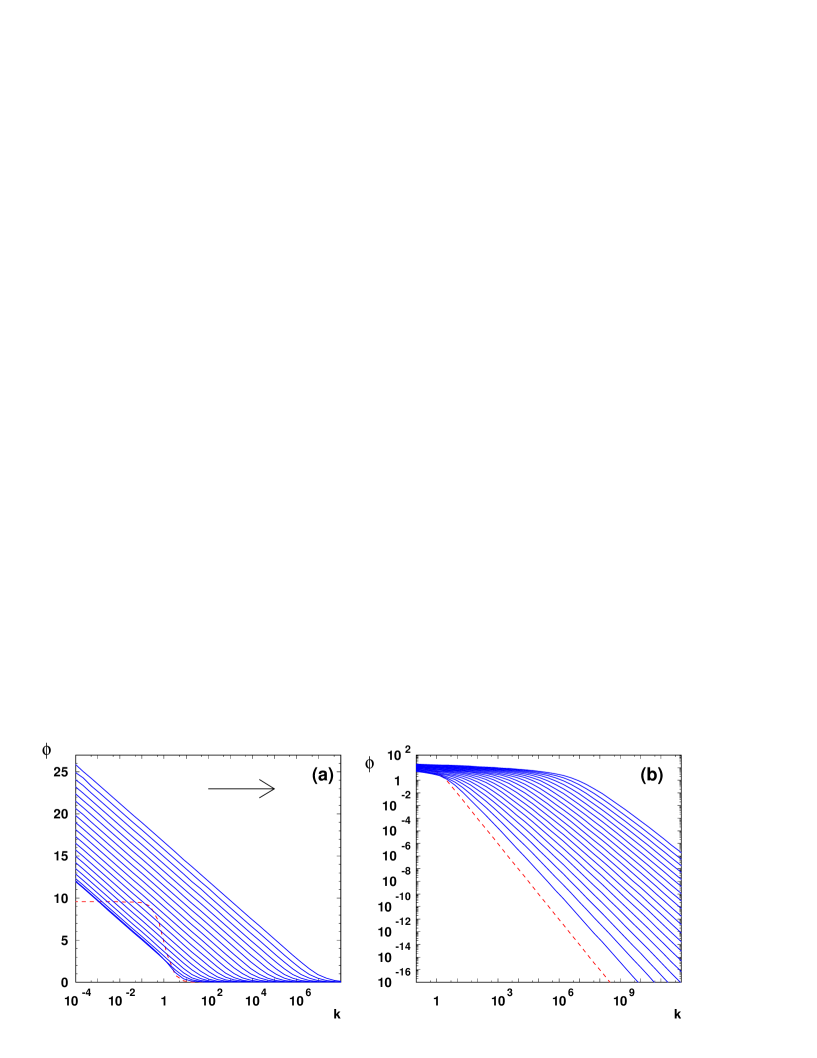
Figure 1: The solution $\phi(Y,k)$ of eq. (1) for twenty values of rapidity from $Y_{0}=0$ to $Y=40$ in the order indicated by the arrow. These are the same plots in the log-lin scale (a), and the log-log scale (b). They illustrate the transition to saturation with decreasing $k$, when the power-like behaviour (b) changes into the logarithmic one (a). The dashed lines is the initial condition with color transparency, $\phi\sim 1/k^{2}$ for large $k$.

How to extract the saturation scale from numerical solutions ? The logarithmic pattern shown in the Fig. 1(a) suggests that after an initial period of the evolution, when details of the initial condition are washed out, the following behaviour sets in

$$\phi(Y,k)=\ln(Q_{s}(Y)/k)\,.$$ (8)

This could be checked numerically if the saturation scale computed from (8), $Q_{s}(Y)=k\exp\{\phi(Y,k)\}$, is independent of $k$. For this purpose we compute $Q_{s}(Y)$ for four different values of $\log_{10}k=-2,-1,0,1$. In this range of $k$ excellent agreement was found, which is shown in Fig. 2(a) where the four saturation scales coincide. All momentum scales are in units of some arbitrary scale $k_{0}$, thus the absolute normalization of the saturation scale is not determined. In order to compare the $Y$-dependence of our saturation scale with the dependence given by eq. (7), we compute the derivative $\partial\ln Q_{s}^{2}/\partial Y$, which is independent of the absolute normalization of $Q_{s}$. The result is shown in Fig. 2(b). The solid lines correspond to the derivative computed from eq. (7) with one, two or three first terms in the asymptotic expansion. The lower dashed line is given by differentiation of the saturation scale defined by eq. (8). We see that such a numerically computed $Q_{s}$ agrees with the expansion (7) with the first two terms. The third term is still not visible at the maximal rapidity achieved in the numerical analysis. It remains to be answered whether this is a numerical effect or the agreement is achieved at higher values of rapidity.

There is another method of computation of the saturation scale, used in most of the analyses based on the linear BFKL equation, i.e. from the equation

$$\phi(Y,Q_{s}(Y))=\phi_{0}\sim 1\,.$$ (9)

This method is more appropriate for the comparison with the Munier–Peschanski analysis since it uses the solution in the wave front region. In Fig. 2(b) the upper dashed curve corresponds to the saturation scale computed from eq. (9), which agrees very well with the three term formula (7).

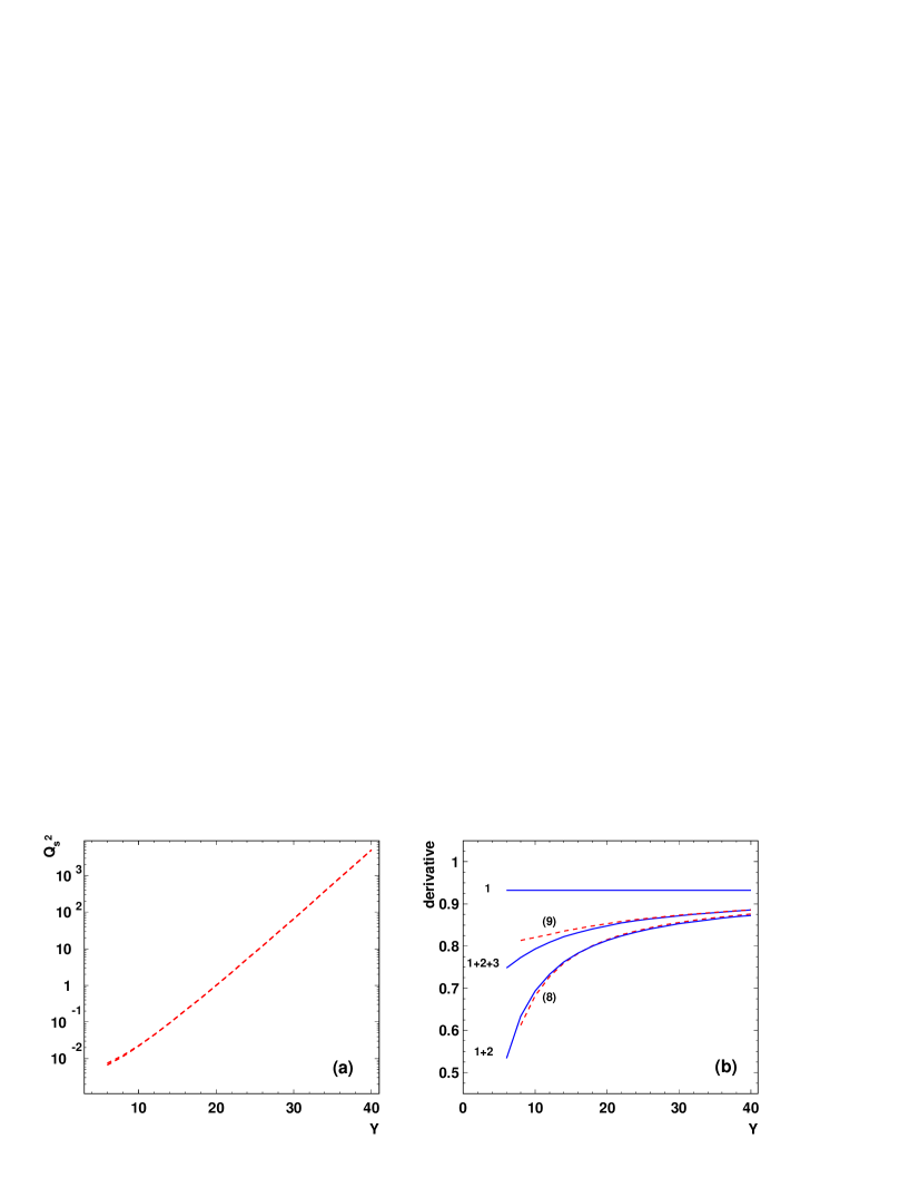
Figure 2: In figure (a) the saturation scale computed from (8) is shown for four values of $k$ given in the text with no visible difference between them. In figure (b) the derivative $\partial\ln Q_{s}^{2}/\partial Y$ is shown. The solid lines correspond to the derivative of the analytic formula (7) with (as indicated) one, two or three terms. The lower dashed line is computed from the saturation scale defined by eq. (8), while the upper dashed line is computed from formula (9).

In conclusion, the analysis of the geometric scaling and saturation scale in the FKKP equation is general and applies to the full nonlinear BK equation.

References

- [1] I. Balitsky, Nucl. Phys. B463, 99 (1996).
- [2] Y. V. Kovchegov, Phys. Rev. D60, 034008 (1999); ibid. D61, 074018 (2000).
- [3] L. V. Gribov, E. M. Levin,M. G. Ryskin, Phys. Rep. 100, 1 (1983).
- [4] L. N. Lipatov Sov. J. Nucl. Phys. 23, 338 (1976); E. Kuraev, L. N. Lipatov and V. S. Fadin JETP 45, 199 (1977); I. I. Balitsky and L. N. Lipatov Sov. J. Nucl. Phys. 28, 822 (1978).
- [5] S. Munier and R. Peschanski, Phys. Rev. Lett. 91, 232001 (2003); Phys. Rev. D69, 034008 (2004).
- [6] A. Staśto, K. Golec-Biernat and J. Kwieciński, Phys. Rev. Lett. 86, 596 (2001).
- [7] S. Munier and R. Peschanski, hep-ph/0401215.