A dynamical gluon mass solution in a coupled system of the Schwinger-Dyson equations

Abstract:

We study numerically the Schwinger-Dyson equations for the coupled system of gluon and ghost propagators in the Landau gauge and in the case of pure gauge QCD. We show that a dynamical mass for the gluon propagator arises as a solution while the ghost propagator develops an enhanced behavior in the infrared regime of QCD. Simple analytical expressions are proposed for the propagators, and the mass dependency on the $\Lambda_{QCD}$ scale and its perturbative scaling are studied. We discuss the implications of our results for the infrared behavior of the coupling constant, which, according to fits for the propagators infrared behavior, seems to indicate that $\alpha_{s}(q^{2})\rightarrow 0$ as $q^{2}\rightarrow 0$.

1 Introduction

Due to the property of asymptotic freedom Quantum Chromodynamics (QCD) has been extensively tested in the regime where high energies are transferred between quarks and gluons. On the other hand we could say that we have only a qualitative understanding of its infrared (IR) properties. Several nonperturbative techniques have been used to study the infrared region, and among these are the QCD simulations on the lattice, which are showing strong evidences that the gluon propagator is infrared finite [1] and that the coupling constant may freeze at low momenta [2].

A possible infrared finite behavior for the gluon propagator and the running coupling constant has also been determined as a solution of the coupled system of Schwinger-Dyson equations (SDE) for the gluon and ghost propagators [3, 4, 5]. Other signals for the freezing of the coupling constant can also be found in the literature [6, 7], and there is an accumulation of phenomenological evidences and possible tests for this soft infrared behavior of the gluon propagator [8] as well as for the coupling constant [9].

In principle the Schwinger-Dyson equations provide a powerful tool to study the QCD infrared behavior, because they comprehend an infinite tower of coupled integral equations that contain all the information about the theory. In practice its intricate structure only become tractable when we make some approximations and truncations. To illustrate the difficulty of this method we notice that only in the nineties, Curtis and Pennington pointed out a truncation scheme, for QED, which is gauge independent and also respect the multiplicative renormalizability [10]. At the moment there are only indications that it is possible to do the same in QCD [11], and, unfortunately, we have to go step by step changing and improving the approximations in order to unravel the actual behavior, or at least to obtain rough solutions that could be compared to other methods like QCD simulations on the lattice.

Recently we solved the SDE for the gluon propagator in the Landau gauge within the so called Mandelstam’s approximation [12]. This is an interesting example of how delicate are these equations.

The gluon propagator within this approximation was first shown to behave as $1/k^{4}$ in the infrared [13], which was appraised as a clear signal of confinement. However this result was discarded by simulations on the lattice [1]. In our previous work [12] assuming a different trilinear gluon vertex and renormalization of the final equation, as suggested by Cornwall [3], and still in agreement with the Mandelstam’s approach, we obtained an infrared finite gluon propagator. Our result showed how the approximations may change the solutions of the SDE. Of course, although the result is very instructive it is not complete because in this approximation the ghosts are neglected. In this work we will improve this approximation with the inclusion of the ghosts fields.

We will solve the coupled SDE for the gluon and ghost propagators in the Landau gauge. Fermions will not be included at this level. As in ref. [12] we follow Cornwall’s prescription to deal with the equation for the gluon propagator. We obtain a numerical solution indicating the generation of a dynamical gluon mass without the introduction of any ansatz for the solutions. The integral equation for the gluon propagator is clearly consistent with a massive gluon polarization operator and its ultraviolet behavior is also consistent with perturbative QCD. The distribution of our paper is the following: In section II we build up the system of coupled equations. In section III we discuss the angular approximation that we perform in the integral equations, which simplifies considerably the amount of numerical work to solve the equations. Section IV contains a discussion of the renormalization procedure and in section V we check the ultraviolet behavior of the equations in order to compare it with the predictions of perturbative QCD. In section VI we present our numerical results and discuss its implications for the infrared behavior of the coupling constant. Our last section contains the conclusion.

2 The coupled SDE for the gluon and ghost propagators

The SDE for the gluon propagator in pure gauge QCD is shown diagrammatically in figure (1). The gluon propagator is written in terms of itself, the full 3 and 4-point gluon vertex $\Gamma_{\mu\nu\rho}$ and $\Gamma_{\mu\nu\rho\sigma}$, and also the full ghost propagator and the gluon-ghost coupling. The ghost propagator depends on itself, on the gluon propagator and also involves the gluon-ghost coupling.

Figure 1: The complete Schwinger-Dyson equation for the gluon propagator without quarks. The spiral lines represent the gluon fields and the dashed lines the ghost fields. The black blobs indicate the full gluon propagators while the white ones represent the full vertices.

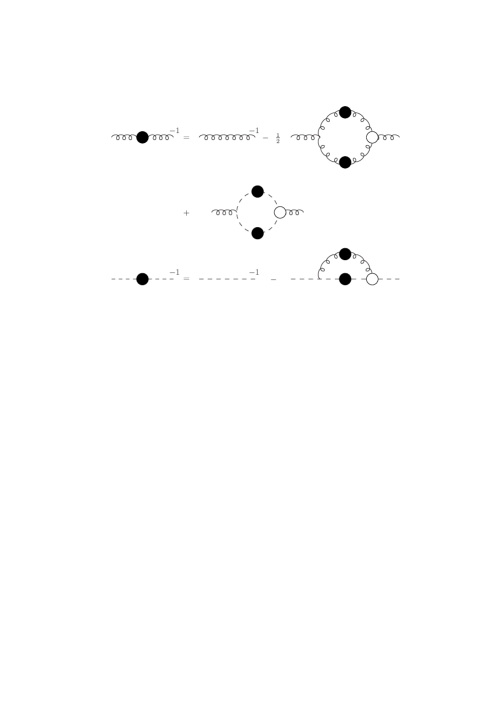
Figure 2: Diagrams for the coupled gluon-ghost system of Schwinger-Dyson equations.

The truncated renormalized SDE for the gluon propagator, in the Landau gauge and at one-loop level, are shown in figure (2) in the same approximation of ref. [4] and it can be written in the Euclidean space as

$$D_{\mu\nu}^{-1}(k)=Z_{3}D^{0}_{\mu\nu}(k) - g^{2}C_{2}\tilde{Z_{1}}\int{\frac{d^{4}q}{(2\pi)^{4}}}iq_{\mu}D_{G}(p)D_{G}(q)G_{\nu}(q,p)$$ (1)

$$+g^{2}C_{2}\frac{1}{2}Z_{1}\int\frac{d^{4}q}{(2\pi)^{4}}\Gamma^{0}_{\mu\rho\alpha}(k,-p,q)D_{\alpha\beta}(q)D_{\rho\sigma}\Gamma_{\beta\sigma\nu}(-q,p,-k),$$

where $p=k+q$, $D^{0}_{\mu\nu}(k)$ and $\Gamma^{0}_{\mu\nu\rho}(p,q,k)$ are the gluon propagator and three gluon vertex at tree level, $\Gamma_{\mu\nu\rho}(p,q,k)$ and $G_{\nu}$ are the full three gluon and gluon-ghost vertices respectively, and we use the color factor $C_{2}=3$. Note that all terms with four-gluon vertices were neglected. One of these contributions is the momentum independent tadpole which can be eliminated by one appropriate choice of the momentum projector as discussed in second paper of ref. [13].

The full gluon propagator that enters into eq.(1) is expressed by

$$D^{\mu\nu}(k)=\frac{\mathcal{Z}(k^{2})}{k^{2}}\left(\delta^{\mu\nu}-\frac{k^{\mu}k^{\nu}}{k^{2}}\right),$$ (2)

where ${\mathcal{Z}(k^{2})}$ is the dressing of the gluon propagator. When ${\mathcal{Z}(k^{2})}=1$ we recover the perturbative expression of the gluon propagator at tree level. Therefore this function measures the transition from the nonperturbative to the perturbative regimes as its value changes with the scale.

It will be useful to introduce here the function $D(k^{2})$ that can be expressed in terms of the dressing of the gluon propagator, ${\mathcal{Z}(k^{2})}$,

$$D(k^{2})=\frac{\mathcal{Z}(k^{2})}{k^{2}},$$ (3)

The full ghost propagator, $D_{G}(k)$, can be defined as

$$D_{G}(k)=-\frac{\mathcal{F}(k^{2})}{k^{2}}.$$ (4)

where ${\mathcal{F}(k^{2})}$ is the dressing of the ghost propagator.

The renormalized SDE for the ghost propagator, shown in figure (2), reads

$$D_{G}^{-1}(k)=-\tilde{Z_{3}}k^{2}+g^{2}C_{2}\tilde{Z_{1}}\int\frac{d^{4}q}{(2\pi)^{4}}ik_{\mu}D_{\mu\nu}(k-q)G_{\nu}(k,q)D_{G}(q).$$ (5)

Note that in the above equations, we have already introduced $Z_{3}$, $\tilde{Z_{3}}$, $Z_{1}$ and $\tilde{Z_{1}}$ which are respectively the renormalization constants for the gluon propagator, the ghost propagator, the three gluon and the gluon-ghost vertices, which are needed in order to render our coupled integral equation system finite. Once the full three gluon and gluon-ghost vertices are known, we have a closed coupled system for the gluon and ghost propagators that can be solved numerically.

The construction of these vertices is based on their respective Slavnov-Taylor identities and its form was discussed in ref. [4]. Apart from a group theoretical factor ($gf^{abc}$) we can express the full three-point vertex function in the following way

$$\Gamma_{\mu\nu\rho}(p,q,k)=-A_{+}(p^{2},q^{2},k^{2})\delta_{\mu\nu}i(p-q)_{\rho}-A_{-}(p^{2},q^{2},k^{2})\delta_{\mu\nu}i(p+q)_{\rho}$$

$$-2\frac{A_{-}(p^{2},q^{2},k^{2})}{p^{2}-q^{2}}(\delta_{\mu\nu}pq-p_{\nu}q_{\mu})i(p-q)_{\rho}+\mbox{c.p.},$$ (6)

where

$$A_{\pm}(p^{2},q^{2},k^{2})=\frac{{\mathcal{F}}(k^{2})}{2}\left(\frac{{\mathcal{F}}(q^{2})}{{\mathcal{F}}(p^{2}){\mathcal{Z}}(p^{2})}\pm\frac{{\mathcal{F}}(p^{2})}{{\mathcal{F}}(q^{2}){\mathcal{Z}}(q^{2})}\right).$$ (7)

The three gluon vertex at tree level can be recovered if we assume that ${\mathcal{Z}}(k^{2})={\mathcal{F}}(k^{2})=1$ and in this way we obtain $A_{-}(p^{2},q^{2},k^{2})=0$ and $A_{+}(p^{2},q^{2},k^{2})=1$.

The full gluon-ghost vertex can be written as [4]

$$G_{\mu}(p,q)=iq_{\mu}\frac{{\mathcal{F}}(k^{2})}{{\mathcal{F}}(q^{2})}+ip_{\mu}\left(\frac{{\mathcal{F}}(k^{2})}{{\mathcal{F}}(q^{2})}-1\right).$$ (8)

Introducing into the eq.(5) the eqs.(2), (4) and (8), we obtain

$$\frac{1}{{\mathcal{F}}(k^{2})}=\tilde{Z_{3}}-g^{2}C_{2}\tilde{Z_{1}}\int\frac{d^{4}q}{(2\pi)^{4}}\,\left(k\mathcal{P}(p)q\right)\,\frac{{\mathcal{Z}}(p^{2}){\mathcal{F}}(q^{2})}{k^{2}\,p^{2}\,q^{2}}\left(\frac{{\mathcal{F}}(p^{2})}{{\mathcal{F}}(q^{2})}+\frac{{\mathcal{F}}(p^{2})}{{\mathcal{F}}(k^{2})}-1\right)\;,$$ (9)

where $p=k-q$ and

$$\mathcal{P}^{\mu\nu}(p)=\delta^{\mu\nu}-\frac{p^{\mu}p^{\nu}}{p^{2}},$$ (10)

is the transversal projector.

Equations (1) and (9) are the coupled SDE equations for the gluon and ghost propagators in the approximation of ref. [4] that we want to solve, following the same steps performed in ref. [12].

3 The angular approximation

In order to solve the coupled system of SDE, compound by the eqs.(1) and (9), shown in the previous section, the first step is to perform the angular integration of the coupled system of integral equations. In our previous work [12], where we considered only the SDE for the gluon propagator and used a specific form for the three gluon vertex, it was simple to compute analytically the angular integration without any approximation. However, in the present case this is not possible anymore and we perform an angular approximation [4] as we explain in the following.

When $q^{2}<k^{2}$ we have that ${\mathcal{F}}(p^{2})={\mathcal{F}}((k-q)^{2})\rightarrow{\mathcal{F}}(k^{2})$ and ${\mathcal{Z}}(p^{2})\rightarrow{\mathcal{Z}}(k^{2})$, that preserves the correct limit when $q^{2}\rightarrow 0$ . On the other hand when we have $q^{2}>k^{2}$ we can set ${\mathcal{F}}(p^{2})\approx{\mathcal{F}}(k^{2})\rightarrow{\mathcal{F}}(q^{2})$. According to this approximation the ghost dressing can be written as

$$\frac{1}{{\mathcal{F}}(k^{2})} = \tilde{Z_{3}}-\frac{9}{4}\lambda\tilde{Z_{1}}\left[\int_{0}^{k^{2}}\frac{dq^{2}}{k^{2}}\frac{q^{2}}{k^{2}}{\mathcal{Z}}(k^{2}){\mathcal{F}}(k^{2})+\int_{k^{2}}^{\Lambda^{2}}\frac{dq^{2}}{q^{2}}{\mathcal{Z}}(q^{2}){\mathcal{F}}(q^{2})\right],$$ (11)

where $\lambda=g^{2}(\mu^{2})/16\pi^{2}$ and the momentum integration in the SDE runs from zero to infinity, and a ultraviolet cutoff $\Lambda$ is introduced to deal with the upper limit of the integrals.

The above equation lead us to

$$\frac{1}{{\mathcal{F}}(k^{2})} = \tilde{Z_{3}}-\frac{9}{4}\lambda\tilde{Z_{1}}\left[\frac{1}{2}{\mathcal{Z}}(k^{2}){\mathcal{F}}(k^{2})+\int_{k^{2}}^{\Lambda^{2}}\frac{dq^{2}}{q^{2}}{\mathcal{Z}}(q^{2}){\mathcal{F}}(q^{2})\right],$$ (12)

while the equation for the gluon propagator now reads

$$\frac{1}{{\mathcal{Z}}(k^{2})}=Z_{3}$$

$$+Z_{1}\lambda\left\{\int_{0}^{k^{2}}\frac{dq^{2}}{k^{2}}\left(\frac{7}{2}\frac{q^{4}}{k^{4}}-\frac{17}{2}\frac{q^{2}}{k^{2}}-\frac{9}{8}\right){\mathcal{Z}}(q^{2}){\mathcal{F}}(q^{2})+\int_{k^{2}}^{\Lambda^{2}}\frac{dq^{2}}{q^{2}}\left(\frac{7}{8}\frac{k^{2}}{q^{2}}-7\right){\mathcal{Z}}(q^{2}){\mathcal{F}}(q^{2})\right\}$$

$$\hskip 85.35826pt+\lambda\left\{\int_{0}^{k^{2}}\frac{dq^{2}}{k^{2}}\frac{3}{2}\frac{q^{2}}{k^{2}}{\mathcal{F}}(k^{2}){\mathcal{F}}(q^{2})-\frac{1}{3}{\mathcal{F}}^{2}(k^{2})+\frac{1}{2}\int_{k^{2}}^{\Lambda^{2}}\frac{dq^{2}}{q^{2}}{\mathcal{F}}^{2}(q^{2})\right\},$$ (13)

where we used the projector

$$\mathcal{R}^{\mu\nu}(k)=\delta^{\mu\nu}-4\frac{k^{\mu}k^{\nu}}{k^{2}},$$ (14)

It is important to mention that to obtain eq.(13), it was neglected one term from the three-gluon loop when $q^{2}<k^{2}$, as discussed at length in the second and third papers of ref.[4].

The above equations are identical to the ones obtained by the authors of ref. [4] in their first calculation of the coupled SDE, and they can be viewed as a natural extension to the gluon SDE in the Mandelstam approximation, since the only difference between the three gluon loop contribution in the previous case and the coupled system is that the gluon dressing function $\mathcal{Z}$ was replaced by the product $\mathcal{Z}G$.

Our system of equations will differ from the one obtained in ref. [4] after the renormalization procedure. One natural question that can arise is how much our solutions will depend on the angular approximation introduced in this section. Obviously, this can only be answered after improving this angular approximation, what we hope to check in the future, however we can say in advance that it is known that in the case of ref. [4] this approximation did not introduce a qualitative change of the solution, but it does produce a quantitative change, specially in the infrared fixed point value of the coupling constant [14].

As we will discuss in detail in the section V, this angular approximation was built in order to recover all the parameters - the gluon and ghost anomalous dimensions and the first order coefficient of the Callan-Symanzik $\beta(g)$ function - that describe the known perturbative behavior of the coupling constant. However we believe that this approximation, despite the fact that it is sucessful in describing the perturbative region [4], can bring some numerical uncertainty in the infrared behavior, which will be reflected in the ratio $m_{0}/\Lambda_{QCD}$, which is a parameter, to be introduced in the section VI, that measures the value of the gluon propagator at zero momentum.

4 Renormalization

As quickly mentioned in the section III, we can link the unrenormalized propagators and vertices with renormalized ones introducing the multiplicative renormalization constants in the following way

$$D_{\mu\nu}^{nr}(q^{2},\Lambda^{2}) = Z_{3}(\mu^{2},\Lambda^{2})D_{\mu\nu}(q^{2},\mu^{2}),$$

$$D_{G}^{nr}(q^{2},\Lambda^{2}) = \tilde{Z_{3}}(\mu^{2},\Lambda^{2})D_{G}(q^{2},\mu^{2}),$$

$$g_{0}^{nr}(\Lambda^{2}) = \tilde{Z_{g}}(\mu^{2},\Lambda^{2})g(\mu^{2}),$$ (15)

where the superscript $nr$ denotes the nonrenormalized quantity and $\mu$ is our renormalization scale. The renormalization constants, in the Landau gauge, are connected through the following relations

$$Z_{1}=Z_{g}Z_{3}^{3/2}\quad\,;\,\quad\tilde{Z_{1}}=Z_{g}Z_{3}^{1/2}\tilde{Z_{3}}.$$ (16)

Furthermore we have one more identity, which is satisfied only in the Landau gauge [15].

To determine the renormalization constants we will impose the following condition on the ghost dressing ${\mathcal{F}}(\mu^{2})=1$, where $\mu$ is chosen in the high energy region, i.e. $\mu>>\Lambda_{QCD}$, where $\Lambda_{QCD}$ is the QCD scale. This procedure is explained in our previous work [12] and is usual when dealing with the SDE [4].

According to this we obtain

$${\mathcal{F}}(\mu^{2})=1,\qquad\rightarrow\qquad\tilde{Z_{3}}=1-\frac{9\lambda}{4}{\mathcal{A}}_{\mathcal{F}}(\mu^{2}),$$ (17)

where ${\mathcal{A}}_{\mathcal{F}}(x)$ is given by

$${\mathcal{A}}_{\mathcal{F}}(x) = \left[\frac{1}{2}{\mathcal{Z}}(x){\mathcal{F}}(x)+\int_{x}^{\Lambda^{2}}\frac{dy}{y}{\mathcal{Z}}(y){\mathcal{F}}(y)\right],$$ (18)

where we substituted $k^{2}$ by $x$ and $q^{2}$ by $y$.

We finally obtain the renormalized expression for the ghost SDE

$${\mathcal{F}}(x)=\left[1-\frac{9}{4}\lambda\left[{\mathcal{A}}_{\mathcal{F}}(x)-{\mathcal{A}}_{\mathcal{F}}(\mu^{2})\right]\right]^{-1},$$ (19)

where ${\mathcal{F}}(x)$ in eq.(19) is now the renormalized ghost dressing.

In the case of the gluon propagator we can rewrite the renormalized eq.(13) in the following compact formula

$${\mathcal{Z}}(x)^{-1}=Z_{3}+\lambda Z_{1}{\mathcal{B}}(x)+\lambda{\mathcal{C}}(x),$$ (20)

where

$${\mathcal{B}}(x)=\int_{0}^{x}\frac{dy}{x}\left(\frac{7y^{2}}{2x^{2}}-\frac{17y}{2x}-\frac{9}{8}\right){\mathcal{Z}}(y){\mathcal{F}}(y)+\int_{x}^{{\Lambda}^{2}}\frac{dy}{y}\left(-7+\frac{7x}{8y}\right){\mathcal{Z}}(y){\mathcal{F}}(y),$$ (21)

and

$${\mathcal{C}}(x)=\int_{0}^{x}\frac{dy}{x}\left(\frac{3y}{2x}\right){\mathcal{F}}(y){\mathcal{F}}(x)+\int_{x}^{\Lambda^{2}}\frac{dy}{2y}{\mathcal{F}}^{2}(y)-\frac{1}{3}{\mathcal{F}}^{2}(x).$$ (22)

The $Z_{3}$ renormalization constant role is to eliminate the divergent terms of the gluon SDE (eq.(20)). Therefore we can add all the potentially divergent terms imposing that

$$xZ_{3}+\frac{1}{2}\lambda\int_{x}^{\Lambda^{2}}{dy}\frac{x}{y}{\mathcal{F}}^{2}(y)-7\lambda\int_{x}^{\Lambda^{2}}dyxD(y){\mathcal{F}}(y)=R+x$$ (23)

where $R$ can be determined through the gluon propagator renormalization condition

$$D^{-1}(\mu^{2})=\mu^{2}\quad\mbox{or}\quad{\mathcal{Z}}(\mu^{2})=1,$$ (24)

where, again, it is worth remembering that the scale $\mu^{2}$ is chosen in the perturbative region. It is important to stress at this point that the subtractive renormalization that we have done above is the same that has been prescribed by Cornwall many years ago [3], and has been explained in detail in ref. [12]. This renormalization allows a massive solution for the gluon propagator. Moreover, as explained in [3] and [12], this approach does not break the Slavnov-Taylor identity involving the gluon propagator and the trilinear gluon vertex as long as we add to the full triple gluon vertex massless pole terms that have been usually neglected in these equations. These terms do not modify the ESD but promote the consistency with the Slavnov-Taylor identities. Finally note that we have not discarded any term from the unrenormalized gluon SDE, but just absorbed the divergent terms in the renormalization constant $Z_{3}$, and that this constant in eq.(23) is proportional do $1$ plus a function of $\mu^{2}$ and $\Lambda^{2}$, which is compatible with the expected weak coupling expansion for this renormalization constant.

In eq.(20) besides the renormalization constant $Z_{3}$ we have some terms multiplied by the constant $Z_{1}$ that comes from the trilinear vertex. We could eliminate this constant in a rigorous way using the relations of eq.(16) such as

$$Z_{1}=\frac{Z_{3}}{\tilde{Z_{3}}}.$$ (25)

which follows from the identity $\tilde{Z_{1}}=1$. However it was shown in ref. [4] that such procedure may destroy the perturbative aspects of the solution within this approximation. As mentioned in our previous work, ref. [12], the SDE renormalization procedure is really an intricate subject and there is not a recipe to deal with these renormalization constants in the nonperturbative region. In such a situation the best that can be done is to go step by step and analyse the consequences of each choice, and we decided in this work to choose the simplest case discussed in ref. [4], $Z_{1}=1$. Using this relation to determine the constant $R$ defined in eq.(23), we obtain the following expression

$$R= - \lambda\int_{0}^{\mu^{2}}dy\left(\frac{7}{2}\frac{y^{2}}{\mu^{4}}-\frac{17}{2}\frac{y}{\mu^{2}}-\frac{9}{8}\right)yD(y){\mathcal{F}}(y)-\frac{3}{2}\lambda\int_{0}^{\mu^{2}}dy\frac{y}{\mu^{2}}{\mathcal{F}}(\mu^{2}){\mathcal{F}}(y)$$ (26)

$$- \lambda\int_{\mu^{2}}^{\Lambda^{2}}dy\frac{7}{8}\frac{\mu^{4}}{y^{2}}yD(y){\mathcal{F}}(y)+\frac{1}{3}\lambda\mu^{2}{\mathcal{F}}^{2}(\mu^{2}).$$

We finally obtain the renormalized SDE equation for the gluon propagator

$$D^{-1}(x)=R+x + \lambda\int_{0}^{x}dy\left(\frac{7}{2}\frac{y^{2}}{x^{2}}-\frac{17}{2}\frac{y}{x}-\frac{9}{8}\right)yD(y){\mathcal{F}}(y)+\frac{3}{2}\lambda\int_{0}^{x}dy\frac{y}{x}{\mathcal{F}}(x){\mathcal{F}}(y)$$ (27)

$$+ \lambda\int_{x}^{\Lambda^{2}}dy\frac{7}{8}\frac{x^{2}}{y^{2}}yD(y){\mathcal{F}}(y)-\frac{1}{3}\lambda x{\mathcal{F}}^{2}(x)$$

where we recall that $\lambda=g^{2}(\mu^{2})/16\pi^{2}$, $x=k^{2}$ and $y=q^{2}$.

It is this last equation, eq.(27), together with the one for the ghost propagator, eq.(19), that will be solved numerically. Note that in eq.(27) as $x\rightarrow 0$ the inverse propagator goes to a constant value, i.e. it shows the presence of a dynamically generated mass.

5 Ultraviolet Behavior

Before solving numerically the coupled SDE it is important to show that they reproduce the QCD perturbative behavior in the high momentum region, confirming the consistency of the renormalization procedure. In order to do so we substitute the perturbative behavior of the gluon and ghost propagators in their respective SDE and keep only the ultraviolet dominant terms in each equation. The solution that comes out are

$$D^{-1}(x)=x\left(1+\frac{\gamma_{0}^{\prime}\alpha(\mu^{2})}{4\pi}\ln\left(\frac{x}{\mu^{2}}\right)\right)\,,$$ (28)

and

$$D_{G}^{-1}(x)=x\left(1+\frac{\delta_{0}^{\prime}\alpha(\mu^{2})}{4\pi}\ln\left(\frac{x}{\mu^{2}}\right)\right).$$ (29)

where $\gamma_{0}^{\prime}=13/2$ and $\delta_{0}^{\prime}=9/4$.

As happened in the case of ref. [12] (see also the discussion of ref. [4]) the momentum behavior of the gluon and ghost propagators is the one expected from perturbative but in addition we recover, in this approximation, the correct perturbative values for the anomalous dimensions ($\gamma_{0}=13/2$ and $\delta_{0}=9/4$ ). Furthemore, we can also obtain the correct value for the first coefficient of the $\beta$ function ($\beta_{0}^{\prime}$).

Starting from the eqs.(15) and (16) we can determine the running coupling constant and $\beta_{0}^{\prime}$. The following relation is satisfied by the renormalized coupling constant

$$g(\mu^{2}) = \frac{Z_{3}^{3/2}(\mu^{2},\Lambda^{2})}{Z_{1}(\mu^{2},\Lambda^{2})}g_{0}^{nr}(\Lambda^{2})$$ (30)

$$= \frac{Z_{3}^{1/2}(\mu^{2},\Lambda^{2})\tilde{Z_{3}}(\mu^{2},\Lambda^{2})}{\tilde{Z_{1}}(\mu^{2},\Lambda^{2})}g_{0}^{nr}(\Lambda^{2}),$$

where the renormalization constants can be obtained from the gluon and ghost dressing functions

$${\mathcal{Z}}^{nr}(x,\Lambda^{2}) = Z_{3}(\mu^{2},\Lambda^{2}){\mathcal{Z}}(x,\mu^{2})$$

$${\mathcal{F}}^{nr}(x,\Lambda^{2}) = \tilde{Z_{3}}(\mu^{2},\Lambda^{2}){\mathcal{F}}(x,\mu^{2}),$$ (31)

leading to the following expression for the coupling constant

$$\alpha_{s}(x,\Lambda^{2})=\alpha_{s}(\mu^{2},\Lambda^{2}){\mathcal{Z}}(x,\mu^{2}){\mathcal{F}}^{2}(x,\mu^{2}).$$ (32)

Inverting the above definition of the coupling constant, using the perturbative definition of the renormalized gluon and ghost functions, which are giving by eqs.(28) and (29) divided by $x$; and keeping only terms $O(\alpha(\mu^{2}))$, we can obtain the following expression

$$\frac{1}{\alpha_{s}(x)}=\frac{1}{\alpha_{s}(\mu^{2})}+\frac{(\gamma_{0}^{\prime}+2\delta_{0}^{\prime})}{4\pi}\ln\left(\frac{x}{\mu^{2}}\right),$$ (33)

where $\beta_{0}^{\prime}=\gamma_{0}^{\prime}+2\delta_{0}^{\prime}=11$, which is identical to the perturbative value ($\beta_{0}=11$). Expressing the eq.(33) in a more familiar way, lead us to

$$\alpha_{s}(x)=\frac{4\pi}{\beta_{0}^{\prime}\ln\left(\frac{x}{\Lambda_{QCD}}\right)},$$ (34)

where $\Lambda_{QCD}$ is the usual QCD scale.

6 Numerical Solution

We can now turn to the numerical calculation to solve the gluon-ghost coupled-system expressed by the eqs.(19) and (27). The solution comes out when we apply an extension of the same iterative numerical method used in ref. [12]. We start defining a logarithmic grid for the $x$ and $y$ variables in order to perform the integration from the deep infrared region to the high energy momenta. This grid is split into two regions, the infrared one $[0,\mu^{2}]$, and the other corresponding to the perturbative region $[\mu^{2},\Lambda^{2}]$. This splitting is needed to impose the renormalization conditions on the dressing functions at the scale $\mu^{2}$.

We then provide initial guesses for the functions $D(x)$ and ${\mathcal{F}}(x)$ and use them to generate the coefficients of the cubic spline interpolation which will produce the values of these functions in terms of the argument $y$. These ones are used in the right hand side of the equation for computing the integral through Adaptive Richardson-Romberg extrapolation.

The initial guesses are compared with the numerical results that were obtained after the integration. The convergence criteria to stop running the numerical code is that the difference between input and output functions must be smaller than $10^{-4}$, otherwise these new numerical results will feed again the right-hand side of the SDE equations and re-start all the procedure until the convergence criteria is satisfied. Using this method we verified that our results are independent of the starting guesses for $D(x)$ and ${\mathcal{F}}(x)$. Our input data are the renormalization point, $\mu^{2}$, and the value of the coupling constant defined at this scale, $\alpha_{s}(\mu^{2})=g^{2}(\mu^{2})/4\pi$, and this will determine the value of $\Lambda_{QCD}$ through the eq.(34). We vary both parameter $\mu^{2}$ and $\alpha_{s}(\mu^{2})$ to scan how our solutions depend on the renormalization point.

We compute the gluon propagator $D(x)$ for various sets of $\mu^{2}$ and $\alpha_{s}(\mu^{2})$ within the range $[10\,\mbox{GeV}^{2},30\,\mbox{GeV}^{2}]$ and $[0.22,0.30]$ respectively as shown in figure (3). We can check through the table(1) that these values correspond to values of $\Lambda_{QCD}$ parameter from $321\,\mbox{MeV}$ to $815\,\mbox{MeV}$. The range of momenta chosen for the scale $\mu^{2}$ is consistent with a perturbative scale and is within the window of squared momenta $10^{-6}$ to $10^{6}$ GeV², which is the maximum range that our calculation can cover without loss of precision in the infrared region.

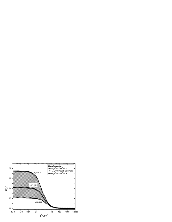
Figure 3: Gluon propagator, $D(q^{2})$, as function of momentum $q^{2}$ for different scales. The line + square curve was obtained when $\alpha_{s}(10\,\mbox{GeV}^{2})=0.25$ which corresponds to $\Lambda_{QCD}=321\,\mbox{MeV}$, while in the line + triangle curve, $\alpha_{s}(30\,\mbox{GeV}^{2})=0.30$, which leads to $\Lambda_{QCD}=815\,\mbox{MeV}$. The shadowed area delimits the curves with $\Lambda_{QCD}$ varying within the range $[321\,\mbox{MeV},815\,\mbox{MeV}]$. The central curve (line + circle) was obtained when we fix the renormalization point, $\mu^{2}$, at the bottom quark mass, $m_{b}^{2}=(4.5)^{2}\,\mbox{GeV}^{2}$ with the central value $\alpha_{s}(m_{b}^{2})=0.22$.

Independently of what is the $\Lambda_{QCD}$ value we can see that all curves in figure (3) develop the same perturbative behavior, on the other hand these curves split in the infrared region going to different values in the limit when the momentum $q^{2}$ goes to zero.

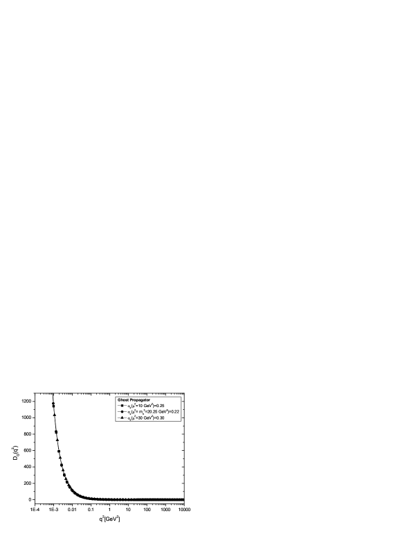
Figure 4: Ghost propagator, $D_{G}(q^{2})$, as function of momentum $q^{2}$ for the same scales shown in the figure (5). The line + square was obtained when $\alpha_{s}(10\,\mbox{GeV}^{2})=0.25$ which corresponds $\Lambda_{QCD}=321\,\mbox{MeV}$, while that in the line + triangle curve, $\alpha_{s}(30\,\mbox{GeV}^{2})=0.30$, which leads to $\Lambda_{QCD}=815\,\mbox{MeV}$. The line + circle was obtained when we fix the renormalization point, $\mu^{2}$, at bottom quark mass, $m_{b}^{2}=(4.5)^{2}\,\mbox{GeV}^{2}$ with the central value $\alpha_{s}(m_{b}^{2})=0.22$. Such curves are obtained varying the $\Lambda_{QCD}$ parameter within the range $[321\,\mbox{MeV},815\,\mbox{MeV}]$.

For the same set of parameters we have also plotted, in the figure (4), the behavior of the ghost propagator as a function of the momentum $q^{2}$. As we can see, for the ghosts, the infrared behavior has a slighter dependence on the renormalization point value than the gluon propagator. In the overall, all curves develop the same behavior from the deep infrared to the high energy region.

In the figures showing the behavior of the gluon and ghost propagators, figures (3) and (4), the most representative curve is the one where the renormalization point, $\mu^{2}$, is set at the bottom quark mass, $m_{b}^{2}=(4.5)^{2}\,\mbox{GeV}^{2}$ with $\alpha_{s}(m_{b}^{2})=0.22$. In this case we obtain a value for $\Lambda_{QCD}=335\,\mbox{MeV}$. We are going to concentrate only in this curve to analyse the perturbative and also non-perturbative regimes, however it is important to keep in mind that it does not really matter what curve we choose to study the high energy regime, since, as mentioned before, all of them have the same perturbative behavior.

For the input discussed above, we plot in figure (5) the gluon propagator, $D(q^{2})$, together with its ultraviolet behavior described by eq.(28) while, in figure (6), we compare the ghost propagator with its ultraviolet behavior expressed by eq.(29). It is interesting to note that, in this latter case, the behavior of the nonperturbative ghost propagator is not so much different from its perturbative behavior, since the major difference starts happening only for $q^{2}$ values less than $2\times 10^{-3}\,\mbox{GeV}^{2}$.

Figure 5: The behavior of the gluon propagator, $D(q^{2})$, obtained through the numerical solution of the Schwinger-Dyson equations, when ${\alpha_{s}(\mu^{2})=0.22}$ at $\mu^{2}=(m_{\mbox{b}})^{2}=(4.5)^{2}\,\mbox{GeV}^{2}$, together with its ultraviolet behavior given by eq.(28) where $\beta_{0}=11$.

Despite the fact that the ghost fields are important to warrant the gluon transversality in the perturbative region and also to recover the first order beta function coefficient and anomalous dimension of the propagators, the above result suggests that neglecting this field, as happens in the Mandelstam approximation, based on an extrapolation from its known small contribution in the perturbative region can be a reasonable approximation.

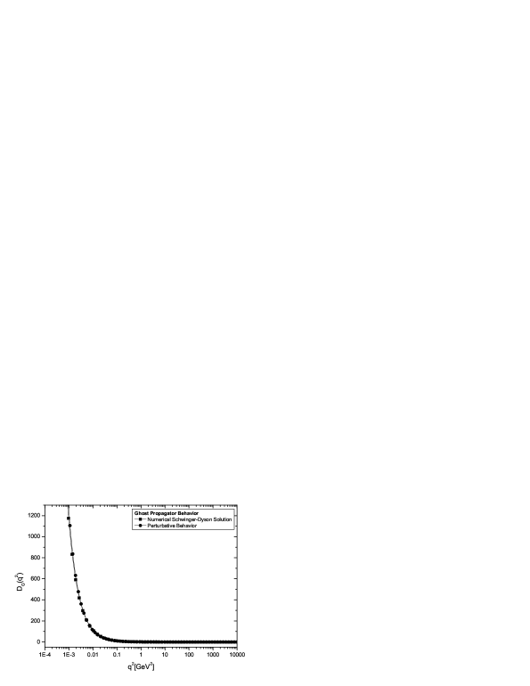
Figure 6: The behavior of the ghost propagator, $D_{G}(q^{2})$, obtained through the numerical solution of the Schwinger-Dyson equation, when ${\alpha_{s}(\mu^{2})=0.22}$ at $\mu^{2}=(m_{\mbox{b}})^{2}=(4.5)^{2}\,\mbox{GeV}^{2}$, together with its ultraviolet behavior given by eq.(29) where $\beta_{0}=11$.

In order to obtain a value for the gluon propagator near $q^{2}=0$, we propose a very simple fit for our numerical data, which in Euclidean space can be written as

$$D(q^{2})=\frac{1}{q^{2}+{\mathcal{M}}^{2}(q^{2})},$$ (35)

and where the dynamical gluon mass ${\mathcal{M}}^{2}(q^{2})$ is described by

$${\mathcal{M}}^{2}(q^{2})=\frac{m_{0}^{4}}{q^{2}+m_{0}^{2}}.$$ (36)

The reason for this fit was discussed in our previous work [12]. In figure (7) the numerical solution for the gluon propagator, determined with the renormalization point fixed at the bottom quark mass, is quite well adjusted with the above fit for $m_{0}^{2}=0.99\,\mbox{GeV}^{2}$. In table (1) the values of $m_{0}^{2}$, utilized in the eq.(36), are shown for each value of the renormalization scale and coupling constant. The value of $m_{0}^{2}$ itself is not important because it is linked to the scale $\Lambda_{QCD}$ through the running of the coupling constant. What really matters is the analysis of the ratio $m_{0}/\Lambda_{QCD}$ which ranges from $1.72$ to $2.97$ and in agreement with previous determinations for this ratio [3, 8]. It is clear that different fits will give slightly different values for the gluon mass, but other choices, as long as they respect the correct asymptotic limits, do not differ appreciably from the values we quoted above. Furthermore the ratio is also relatively stable against variations of the renormalization point.

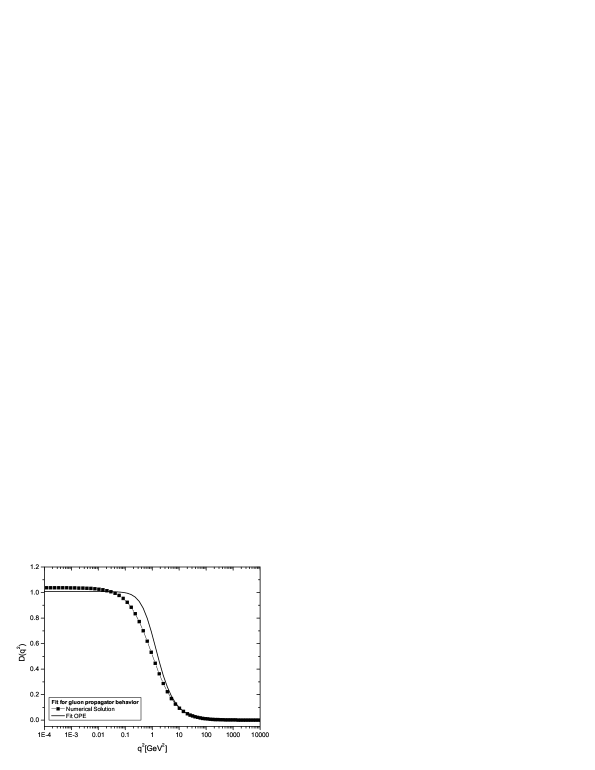
Figure 7: Numerical solution for the gluon propagator, $D(q^{2})$, versus momentum $p^{2}$ for $\alpha_{s}(m^{2}_{b})=0.22$. We compare this numerical solution with the fit given by eq.(35), where $m_{0}^{2}=0.99\,\mbox{GeV}^{2}$.

We can also discuss the behavior of the coupling constant in the infrared. In order to do so we start remembering that the running coupling constant is given by eq.(32), where the gluon and ghost dressing functions are utilized as input. Note that if we assume the fit given by eq.(35) for the gluon propagator and roughly approximate the ghost dressing function by $1$, because in the full region of momenta its behavior is almost the perturbative one as can be seen in figure (6), we clearly obtain a vanishing coupling in the deep infrared region. Since the major difference between the nonperturbative and the perturbative behavior of the ghost propagator starts happening for $q^{2}$ values less than $2\times 10^{-3}$, instead of the rough approximation ${\mathcal{F}}(x)\approx 1$ in the low momenta region we introduce the following fits: ${\mathcal{F}}(x)=(x/m_{0}^{2})^{\eta}$ for the ghost dressing function, and ${\mathcal{Z}(x)}=(x/(x+m_{0}^{2}))^{\delta}$ for the gluon dressing function, in the region delimited by $q^{2}<0.1\,\mbox{GeV}^{2}$. These exponents provide additional freedom to our fits, and we are able to fit the data with $\eta=-0.04$ and $\delta=0.98$. These figures confirm the same vanishing behavior of the coupling constant in the deep infrared region previously examined, in the context of lattice QCD simulation, by the authors of Ref.[16].

$\alpha(\mu^{2})\quad$ $\mu^{2}$ $\Lambda_{QCD}\quad$ $m_{0}^{2}$ $m_{0}/\Lambda_{QCD}$ $(\beta=11)\quad$ $0.22\quad$ $20.25\,\mbox{GeV}^{2}$ $335\,\mbox{MeV}\quad$ $0.99\,\mbox{GeV}^{2}$ $2.97\,\qquad$ $0.25\quad$ $10\,\mbox{GeV}^{2}$ $321\,\mbox{MeV}\quad$ $0.55\,\mbox{GeV}^{2}$ $2.31\,\qquad$ $0.25\quad$ $20\,\mbox{GeV}^{2}$ $455\,\mbox{MeV}\quad$ $1.10\,\mbox{GeV}^{2}$ $2.31\,\qquad$ $0.25\quad$ $30\,\mbox{GeV}^{2}$ $557\,\mbox{MeV}\quad$ $1.65\,\mbox{GeV}^{2}$ $2.31\,\qquad$ $0.30\quad$ $10\,\mbox{GeV}^{2}$ $471\,\mbox{MeV}\quad$ $0.65\,\mbox{GeV}^{2}$ $1.72\,\qquad$ $0.30\quad$ $20\,\mbox{GeV}^{2}$ $666\,\mbox{MeV}\quad$ $1.31\,\mbox{GeV}^{2}$ $1.72\,\qquad$ $0.30\quad$ $30\,\mbox{GeV}^{2}$ $815\,\mbox{MeV}\quad$ $1.96\,\mbox{GeV}^{2}$ $1.72\,\qquad$

Table 1: Values of the renormalization point, $\mu^{2}$, and coupling constant, $\alpha(\mu^{2})$, used as input data in the eqs.(19) and (27). These values fix automatically, through eq.(34), the $\Lambda_{QCD}$ scale. In the third column, we have the values of $\Lambda_{QCD}$ computed with our perturbative value of $\beta_{0}=11$. The values for the ratio $m_{0}/\Lambda_{QCD}$ are also shown in the last column where the $m_{0}^{2}$ values are defined through eq.(36).

7 Conclusions

We solved the coupled system of Schwinger-Dyson equations for the gluon and ghost propagators in the Landau gauge in the case of pure gauge QCD. The new ingredient in our approach is that we use a renormalization prescription formulated by Cornwall many years ago which allows for a dynamically generated mass. As explained in a previous work this solution is compatible with the Slavnov-Taylor identities when a new piece containing massless poles is added to the triple gluon full vertex. The renormalization constant has the form $Z_{3}=1+f(\mu^{2},\Lambda^{2})$ which is consistent with the weak coupling expansion of this constant. The ratio between the dynamical gluon mass and $\Lambda_{QCD}$ is also consistent with previous determinations.

To obtain the SDE solutions we do not need any ansatz for the asymptotic equation and we are able to solve them numerically in a quite large range of momenta. The numerical solutions are quite stable and we could, as we did in ref. [12], compute an effective potential for composite operators to show that we also obtain a reasonable value for the gluon condensate, although this calculation is a little bit redundant because the gluon propagator do not differ appreciably from the one that we obtained in the previous work. It seems that in the present case the inclusion of ghosts induces only a minor numerical modification of the previous result. We present simple fits for the gluon and ghost propagator and discuss the infrared behavior of the running coupling constant. These fits allow us to study the behavior of the running coupling in the deep infrared region, and indicate that the running coupling goes to zero when $q^{2}\rightarrow 0$.

There are many points that still must be improved in the present approach. We need to compute the equations without the angular approximation. A different approximation, other than $Z_{1}=1$ must be tested. The inclusion of fermions and the tadpole diagram are among the many other modifications that must be considered in the future.

8 Acknowledgments

We benefited from discussions with A. Cucchieri and G. Krein and we would also like to thank A. Colato for his numerical hints. This research was supported by the Conselho Nacional de Desenvolvimento Científico e Tecnológico (CNPq) (AAN) and by Fundação de Amparo à Pesquisa do Estado de São Paulo (FAPESP) (ACA).

References

- [1] P. Marenzoni, G. Martinelli, N. Stella, e M. Testa, Phys. Lett. B318 (1993) 511; C. Alexandrou, Ph. de Forcrand and E. Follana, Phys. Rev. D65 (2002) 114508; D65 (2002) 117502; F. D. R. Bonnet et al., Phys. Rev. D64 (2001) 034501; D62 (2000) 051501; D. B. Leinweber et al. (UKQCD Collaboration), Phys. Rev. D58 (1998) 031501; C. Bernard, C. Parrinello, and A. Soni, Phys. Rev. D49 (1994) 1585; see also the most recent simulation of P. O. Bowman et al., hep-lat/0402032 and the references therein.
- [2] A recent study about the freezing of the coupling constant in a SU(2) gauge theory with references to QCD simulations can be found in J. C. R. Bloch, A. Cucchieri, K. Langfeld and T. Mendes, hep-lat/0312036; Nucl. Phys. Proc. Suppl. 119 (2003) 736.
- [3] J. M. Cornwall, Phys. Rev. D26 (1982) 1453; J. M. Cornwall and J. Papavassiliou, Phys. Rev. D40 (1989) 3474; D44 (1991) 1285.
- [4] R. Alkofer and L. von Smekal, Phys. Rept. 353 (2001) 281; L. von Smekal, A. Hauck and R. Alkofer, Ann. Phys. 267 (1998) 1; A. Hauck, L. von Smekal and R. Alkofer, Comput. Phys. Commun. 112 (1998) 166; L. vonSmekal, A. Hauck and R. Alkofer, Phys. Rev. Lett. 79 (1997) 3591.
- [5] K.-I. Kondo, hep-th/0303251.
- [6] D. V. Shirkov and I. L. Solovtsov, Phys. Rev. Lett. 79 (1997) 1209; D. V. Shirkov, Eur. Phys. J. C22 (2001) 331; D.V. Shirkov, Theor. Math. Phys. 132 (2002) 1309; V. N. Gribov, Nucl. Phys. B139 (1978) 1; see also the interesting review by Y. L. Dokshitzer and D. E. Kharzeev, hep-ph/0404216 where the Gribov’s results about infrared finite gluon propagator and coupling constant are revisited.
- [7] A. C. Aguilar, A. A. Natale and P. S. Rodrigues da Silva, Phys. Rev. Lett. 90 (2003) 152001.
- [8] F. Halzen, G. Krein and A. A. Natale, Phys. Rev. D47 (1993) 295; M. B. Gay Ducati, F. Halzen and A. A. Natale, Phys. Rev. D48 (1993) 2324; A. Mihara and A. A. Natale, Phys. Lett. B482 (2000) 378; A. C. Aguilar, A. Mihara and A. A. Natale, Int. J. Mod. Phys. 19 (2004) 249.
- [9] A. C. Mattingly and P. M. Stevenson, Phys. Rev. D49 (1994) 437; Y. L. Dokshitzer, G. Marchesini and B. R. Webber, Nucl. Phys. B469 (1996) 93; Y. L. Dokshitzer, in Proc. 29th Int. Conf. on High Energy Physics (ICHEP 98), Vancouver, Canada, 1998, High energy physics, Vol.1, p. 305, hep-ph/9812252; S. J. Brodsky, hep-ph/0310289; A. C. Aguilar, A. Mihara and A. A. Natale, Phys. Rev. D65 (2002) 054011.
- [10] D. C. Curtis and M. R. Pennington, Phys. Rev. D42 (1990) 4165.
- [11] See J. C. R. Bloch, Few. Body Syst. 33 (2003) 111 and references therein.
- [12] A. C. Aguilar and A. A. Natale, hep-ph/0405024
- [13] S. Mandelstam, Phys. Rev. D20 (1979) 3223; N. Brown and M. R. Pennington, Phys. Rev. D38 (1988) 2266; Phys. Rev. D39 (1989) 2723.
- [14] D. Atkinson and J. C. R. Bloch, Mod. Phys. Lett. A13 (1998) 1055.
- [15] J. C. Taylor, Nucl. Phys. B33 (1971) 436.
- [16] P. Boucaud, J. P. Leroy, J. Micheli, O. Pene and C. Roiesnel, JHEP 10 (1998) 17; P. Boucaud et al. JHEP 201 (2002) 46; Nucl. Phys. Proc. Suppl. 106 (2002) 266.