Abstract

The mass of the Higgs boson in the Split Supersymmetric Standard Model is calculated, including all one-loop threshold effects and the renormalization group evolution of the Higgs quartic coupling through two-loops. The two-loop corrections are very small ($\ll 1\;{\rm GeV}$), while the one-loop threshold corrections generally push the Higgs mass down several ${\rm GeV}$.

1 Introduction

The gauge hierarchy problem of the standard model (SM) of particle physics has been a fruitful source of inspiration for beyond the SM physics. Most notably, a main reason for the prominence of supersymmetry was its natural solution to this problem. In recent years, additional circumstantial evidence for supersymmetry (SUSY) has arisen from gauge coupling unification and from dark matter, although these successes have been partially offset by difficulties with flavor changing neutral currents and CP violation which arise from light SUSY scalars. Thus, it may be reasonable to abandon the original motivation for SUSY and consider the implications of a theory which maintains all of the successes of the MSSM, except for the hierarchy problem, and does away with some of the difficulties. This proposal, called finely tuned, or split supersymmetry, has appeared in [1][2], and some phenomenology has been discussed [3, 4, 5, 6, 7, 8, 9]. In split supersymmetry, a single Higgs scalar is fine tuned to be light, with the understanding that the fine tuning will be resolved by some anthropic-like selection effects. This approach may have a natural realization within inflation and string theory [10], where an almost infinite landscape of vacua may contain a small percentage which have the desired fine-tuned parameters necessary for life and the properties of our universe.

The prediction for the Higgs boson mass is typically higher in Split SUSY than MSSM scenarios, and is thus a key distinguishing feature. The MSSM Higgs mass is known to two-loop accuracy [11]. The purpose of this paper is to bring the split supersymmetry Higgs mass prediction to a similar level of precision.

2 Corrections to the Higgs Mass

The starting point for our analysis is the split SUSY Lagrangian [1][2]

$${\cal L} = m^{2}H^{\dagger}H-\frac{\lambda}{2}(H^{\dagger}H)^{2}+F_{U}\hat{H}^{\dagger}Q\overline{u}+F_{D}H^{\dagger}Q\overline{d}+F_{L}H^{\dagger}L\overline{e}+{\rm h.c.}$$ (1)

$$- \frac{M_{1}}{2}\widetilde{B}\widetilde{B}-\frac{M_{2}}{2}\widetilde{W}^{I}\widetilde{W}^{I}-\frac{M_{3}}{2}\widetilde{g}^{a}\widetilde{g}^{a}-\mu\widetilde{H}^{T}_{u}\epsilon\widetilde{H}_{d}$$

$$- \frac{H^{\dagger}}{\sqrt{2}}\Big{(}\kappa_{u}\sigma^{I}\widetilde{W}^{I}+\kappa_{u}^{\prime}\widetilde{B}\Big{)}\widetilde{H}_{u}+\frac{\hat{H}^{\dagger}}{\sqrt{2}}\Big{(}-\kappa_{d}\sigma^{I}\widetilde{W}^{I}+\kappa_{d}^{\prime}\widetilde{B}\Big{)}\widetilde{H}_{d}+{\rm h.c.},$$

where $\hat{H}=-i\sigma_{2}H^{*}$, $H=(H^{+},H^{0})^{T}$, and $\epsilon=i\sigma_{2}$. The predictions for the Higgs mass will be derived from this Lagrangian using methods similar to the work of Sirlin and Zucchini on the SM Higgs boson [12] and the subsequent work of Hempfling and Kniehl on the SM top quark [13].

After electroweak symmetry breaking, the bare Higgs mass is related to the bare quartic coupling $\lambda_{0}$ and vacuum expectation value (vev) $v_{0}=\sqrt{2}\langle H^{0}\rangle$ by

$$M_{h_{0}}(\overline{\mu})=\sqrt{\lambda_{0}(\overline{\mu})}v_{0}(\overline{\mu})$$ (2)

where the dimensional regularization scale $\overline{\mu}$ is introduced into loop integrals through $\int d^{4}x\rightarrow\overline{\mu}^{-2\epsilon}\int d^{d}x$ and is elevated to the renormalization scale in $\overline{MS}$. Each of these bare quantities must be related to physical quantities in order to obtain a meaningful relation.

The pole mass is related to the bare mass by

$$M_{h}^{2}=M_{h_{0}}^{2}(\overline{\mu})+{\rm Re~{}}\Sigma_{h}(M_{h},\overline{\mu})+3\frac{T_{h}(\overline{\mu})}{v},$$ (3)

where $\Sigma_{h}$ is the Higgs self energy and $T_{h}$ is the tadpole. The bare vev is related to the renormalized vev via muon decay [14] :

$$v_{0}^{2}(\overline{\mu})=v_{F}^{2}\Bigg{(}1+\Pi_{WW}(0,\overline{\mu})+E(\overline{\mu})-2\frac{T_{h}(\overline{\mu})}{M_{H}^{2}v_{F}}\Bigg{)},$$ (4)

where $v_{F}=1/\sqrt{\sqrt{2}G_{F}}\;\approx\;246.22{\rm GeV}$, $\Pi_{WW}(0,\overline{\mu})$ is the $W^{\pm}$ boson self-energy at zero momentum, and $E$ represents vertex and box corrections to muon decay in the standard model. Finally the bare coupling is related to the $\overline{MS}$ coupling by

$$\lambda_{0}(\overline{\mu})=\lambda(\overline{\mu})+\frac{\beta_{\lambda}}{2}C_{UV},$$ (5)

where $C_{UV}=\frac{1}{\epsilon}-\gamma_{E}+\log{4\pi}$ and $\beta_{\lambda}=\frac{\partial\lambda}{\partial\log{\overline{\mu}}}$. Putting these together, one finds

$$M_{h} = \sqrt{\lambda(\overline{\mu})}v_{F}\big{(}1+\delta_{h}(\overline{\mu})\big{)}$$

$$\delta_{h}(\overline{\mu}) = {\litfont{1\over 2}}\left({{\rm Re~{}}\Sigma_{h}(M_{h},\overline{\mu})\over M_{h}^{2}}+\frac{T_{h}(\overline{\mu})}{M_{h}^{2}v_{F}}+E(\overline{\mu})+\Pi_{WW}(0,\overline{\mu})+\frac{\beta_{\lambda}}{2\lambda}C_{UV}\right).$$ (6)

This formula includes all one-loop threshold and renormalization group (RG) corrections, and can be improved to include the two-loop RG corrections to the running of $\lambda(\overline{\mu})$. The scale $\overline{\mu}$ should be chosen to minimize large logarithmic corrections, although at one-loop the $\overline{\mu}$ (and $C_{UV}$) dependence formally cancels from Eq.(2). The results for $\delta_{h}(\overline{\mu})$ in the SM were given in [12]. The split supersymmetry threshold corrections are discussed in detail in section 2.5.

2.1 The algorithm used to calculate the Higgs mass

The input parameters for the Higgs mass analysis include supersymmetry breaking scale $M_{S}$, $\tan{\beta}$ at $M_{S}$, and the soft gaugino and higgsino masses $M_{1}$, $M_{2}$, $M_{3}$, and $\mu$ (not to be confused with the RN scale $\overline{\mu}$) which are specified at the scale of gauge coupling unification $M_{G}\sim 3\times 10^{16}{\rm GeV}$ and are assumed to be universal

$$M_{1/2}\equiv M_{1}(M_{G})=M_{2}(M_{G})=M_{3}(M_{G})=\mu(M_{G}).$$ (7)

Of course, the $\mu$-term may take different values from the gaugino masses, but we have explicitly verified that the Higgs mass prediction is very insensitive to the $\mu$ initial value, so the results in Figs.(1-4) are valid for most other reasonable values of $\mu$.

First, the coupled system of differential equations [2] for $g_{1}$, $g_{2}$, $g_{3}$, $F_{U}$, $F_{D}$, $F_{L}$, $\kappa_{u}$, $\kappa_{d}$, $\kappa_{u}^{\prime}$, $\kappa_{d}^{\prime}$ are solved numerically. The gauge couplings are run at two loops, whereas the seven other couplings are run at one loop. We keep only the top, bottom, and tau Yukawa couplings and so can replace $F_{U}\rightarrow Y_{t},F_{D}\rightarrow Y_{b},F_{L}\rightarrow Y_{\tau}$ in the all of the following formulae. The boundary values of the gauge couplings $g_{1},g_{2},g_{3}$ and Yukawa couplings $Y_{b},Y_{\tau}$ are given at scale $M_{Z}$ from the latest world averages [15]. As will be discussed in section 2.3, $Y_{t}$ is given at the top pole mass $M_{t}$, including three-loop QCD corrections and one-loop threshold corrections from electro-weak and split supersymmetric interactions. The new split SUSY Yukawas are given at scale $M_{S}$ through the relations:

$$\kappa_{u}(M_{S}) = g_{2}(M_{S})\sin{\beta}$$

$$\kappa_{d}(M_{S}) = g_{2}(M_{S})\cos{\beta}$$

$$\kappa_{u}^{\prime}(M_{S}) = \sqrt{\frac{3}{5}}g_{1}(M_{S})\sin{\beta}$$

$$\kappa_{d}^{\prime}(M_{S}) = \sqrt{\frac{3}{5}}g_{1}(M_{S})\cos{\beta}.$$ (8)

Because the boundary values for the couplings are given at different scales, it is necessary to take an iterative approach to solving the differential equations. The couplings which are specified at low scales, such as $y_{t}(M_{t})$, are guessed at the high scale $M_{s}$, the differential equations are then solved, and the resulting value for $y_{t}(M_{t})$ is compared to the correct value in order to obtain a better guess, at which point the procedure is repeated. Five iterations are usually sufficient. An additional complication arises because the split SUSY corrections to $Y_{t}(M_{t})$ (detailed in section 2.3) depend on $U,V,$ and $N$, which depend on the solutions of the RGE’s for the gaugino/higgsino masses, which depend on the solutions of the RGE’s for the dimensionless couplings, which in turn depend upon $Y_{t}(M_{t})$. Thus, this entire analysis should be performed iteratively.

Armed with the RGE evolution of the dimensionless couplings, the RGE’s for the soft masses $M_{1}$, $M_{2}$, $M_{3}$, and $\mu$ are then solved and are run down to scales $M_{1}$, $M_{2}$, $M_{3}$, and $\mu$, respectively, where the physical pole masses are extracted, as detailed in section 2.2. The chargino and neutralino mixing matrices $U,V,$ and $N$ will appear in the threshold corrections.

In section 2.4 the two-loop running of the Higgs quartic coupling will be given. The solutions for $g_{1}$, $g_{2}$, $g_{3}$, $F_{U}$, $F_{D}$, $F_{L}$, $\kappa_{u}$, $\kappa_{d}$, $\kappa_{u}^{\prime}$, $\kappa_{d}^{\prime}$ yield the required inputs to solve the $\lambda$ RGE, with the gaugino and higgsino masses providing the appropriate matching scale between the Standard Model and split supersymmetric running. The boundary value of the Higgs quartic coupling in minimal split supersymmetry is

$$\lambda(M_{S})=\frac{1}{4}\Bigg{(}g_{2}^{2}(M_{S})+\frac{3}{5}g_{1}^{2}(M_{S})\Bigg{)}\cos^{2}{2\beta}.$$ (9)

Finally, all that remains is to include the finite threshold corrections in Eq.(2). These are detailed in section 2.5. Results for the Higgs mass are given in section 3.

2.2 The gaugino and higgsino mass spectrum

The formulae for the running of the gaugino and higgsino masses are given in Eqs.(57-63) of Ref.[2].

The gluino mass appears in our analysis as the threshold for the running of the strong coupling. It is straightforward to evaluate $M_{3}$ at scale $M_{3}$ and deduce the pole mass

$$M_{\widetilde{g}}=M_{3}(M_{3})\left(1+12\;\frac{g_{3}^{2}(M_{3})}{(4\pi)^{2}}\right).$$ (10)

The chargino and neutralino mass matrix diagonalization proceeds similar to the MSSM [16]. The mass matrices are given by

$$X=\Bigg{(}\matrix{M_{2}&\frac{\kappa_{u}v}{\sqrt{2}}\cr\frac{\kappa_{d}v}{\sqrt{2}}&\mu}\Bigg{)}\;\;\;\;\;\;\;\;\;\;Y=\left(\begin{array}[]{cccc}M_{1}&0&-\frac{\kappa_{d}^{\prime}v}{\sqrt{2}}&\frac{\kappa_{u}^{\prime}v}{\sqrt{2}}\\ 0&M_{2}&\frac{\kappa_{d}v}{\sqrt{2}}&-\frac{\kappa_{u}v}{\sqrt{2}}\\ -\frac{\kappa_{d}^{\prime}v}{\sqrt{2}}&\frac{\kappa_{d}v}{\sqrt{2}}&0&-\mu\\ \frac{\kappa_{u}^{\prime}v}{\sqrt{2}}&-\frac{\kappa_{u}v}{\sqrt{2}}&-\mu&0\end{array}\right)$$ (11)

These are diagonalized by matrices $U,V$ in the chargino sector ($\chi_{i}^{+}\chi_{i}^{-}$) and $N$ in the neutralino sector ($\chi_{i}^{0}$):

$$\chi_{i}^{+}=V_{ij}\psi_{j}^{+}\;\;\;\;\;\chi_{i}^{-}=U_{ij}\psi_{j}^{-}\;\;\;\;\chi_{i}^{0}=N_{ij}\psi_{j}^{0},$$ (12)

where the gauge eigenstates are

$$\psi_{j}^{+}=\Bigg{(}\matrix{\widetilde{W}^{+}\cr\widetilde{H}_{u}^{+}}\Bigg{)}\;\;\;\;\;\;\psi_{j}^{-}=\Bigg{(}\matrix{\widetilde{W}^{-}\cr\widetilde{H}_{d}^{-}}\Bigg{)}\;\;\;\;\;\;\psi_{j}^{0}=(\widetilde{B},\widetilde{W}_{3},\widetilde{H}_{d}^{0},\widetilde{H}_{u}^{0})^{T}.$$ (13)

The matrices $U,V,N$ are specified by

$$N^{*}YN^{-1}=M^{(N)} = {\rm diag}\{M^{(N)}_{1},M^{(N)}_{2},M^{(N)}_{3},M^{(N)}_{4}\}$$

$$NY^{\dagger}YN^{-1} = (M^{(N)})^{2}$$

$$U^{*}XV^{-1} = M^{(C)}={\rm diag}\{M^{(C)}_{1},M^{(C)}_{2}\}$$

$$VX^{\dagger}XV^{-1} = (M^{(C)})^{2}=U^{*}XX^{\dagger}U^{T}$$ (14)

The running mass parameters $M_{1}$, $M_{2}$, $\mu$ are evaluated at the scales $M_{1}$, $M_{2}$, $\mu$, respectively, in an iterative fashion. This minimizes the threshold corrections relating the pole masses and running masses, which are not considered in detail. In any case, the results are very insensitive to the exact scale chosen. The threshold effects due to gaugino masses are incorporated into the running of the dimensionless parameters appropriately.

2.3 The Top Quark Yukawa coupling and pole mass

Since the Higgs mass is most sensitive to the top Yukawa coupling, it is important to carefully extract this from the pole mass, which is taken from the 2005 summer average of CDF and D0 [17] to be $M_{t}=172.7\pm 2.9\;{\rm GeV}$. The leading corrections are from QCD, and were calculated to two-loops in [18] and to three-loops in [19]. The full electro-weak corrections at one-loop were considered in [13], where the authors found the following relation between the pole mass, the $\overline{MS}$ Yukawa coupling, and the vacuum-expectation-value $v_{F}$ :

$$y_{t}(\overline{\mu})=\sqrt{2}\frac{M_{t}}{v_{F}}\Big{(}1+\delta_{t}(\overline{\mu})\Big{)}.$$ (15)

The correction term is derived analogous to Eq.(2) and is given by

$$\delta_{t}(\overline{\mu})={\rm Re}{\Sigma_{t}(M_{t},\overline{\mu})}-\frac{\Pi_{WW}(0,\overline{\mu})}{2M_{W}^{2}}-\frac{E(\overline{\mu})}{2}-\frac{\beta_{y_{t}}}{2y_{t}}C_{UV}.$$ (16)

In this formula, $\Sigma_{t}$ represents the top quark self energy and $E$ is the vertex and box corrections to muon decay, neither of which receive new contributions in split SUSY at one-loop. However, the $W$ boson self energy, $\Pi_{WW}$, does receive corrections, which are calculated below. The UV divergence, $C_{UV}$, multiplying the top Yukawa beta function $\beta_{y_{t}}=\overline{\mu}\frac{\partial y_{t}}{\partial\overline{\mu}}$ comes from the relation between the bare and $\overline{MS}$ Yukawa coupling and is canceled by the divergent parts of $\Sigma_{t},\Pi_{WW},$ and $E$.

It is convenient to decompose the correction term into parts arising from QCD, electro-weak theory (EW), and split-supersymmetry (SS) :

$$\delta_{t}(\overline{\mu})=\delta_{t}^{QCD}(\overline{\mu})+\delta_{t}^{EW}(\overline{\mu})+\delta_{t}^{SS}(\overline{\mu})$$ (17)

The three-loop QCD term derived from [18][19] for the top quark at scale $\overline{\mu}=M_{t}$ is

$$\delta_{t}^{QCD}(\overline{\mu}=M_{t}) \approx -{4\over 3}\left({\alpha_{3}(M_{t})\over\pi}\right)-9.1\;\left({\alpha_{3}(M_{t})\over\pi}\right)^{2}-80\;\left({\alpha_{3}(M_{t})\over\pi}\right)^{3}$$ (18)

$$\approx -0.046-0.011-0.003\approx-0.060$$

for $\alpha_{3}(M_{Z})=0.118$. While the EW term given in Ref.[13] formally depends on $M_{h}$ and $M_{t}$, it turns out that in the range of Higgs and top masses of interest, this contribution is negligible $|\delta_{t}^{EW}|<0.001$.

Now we turn to the SS corrections, which arise only from the gaugino and higgsino contribution to the $W^{\pm}$ self-energy. The $W^{\pm}-\chi^{0}_{i}-\chi^{\pm}_{j}$ vertex is given by $ig\gamma_{\mu}(L_{ij}P_{L}+R_{ij}P_{R})$, with

$$L_{ij} = -\frac{1}{\sqrt{2}}N_{i4}V^{*}_{j2}+N_{i2}V^{*}_{j1}$$

$$R_{ij} = \frac{1}{\sqrt{2}}N^{*}_{i3}U_{j2}+N^{*}_{i2}U_{j1}.$$ (19)

This vertex is used to derive the split SUSY corrections involving charginos and neutralinos :

$$16\!\!\!\! \pi^{2} \!\!\!\!\Pi_{WW}^{(C,N)}(0,\overline{\mu})=-2M_{W}^{2}C_{UV}X_{2}(SS)$$

$$+ g^{2}\sum_{i=1}^{4}\sum_{j=1}^{2}\Bigg{(}(L_{ij}L_{ij}^{*}+R_{ij}R_{ij}^{*})\left[a^{2}\left(\log{a^{2}\over\overline{\mu}^{2}}-1/2\right)+b^{2}\left(\log{b^{2}\over\overline{\mu}^{2}}-1/2\right)+{a^{2}b^{2}\over a^{2}-b^{2}}\log{a^{2}\over b^{2}}\right]$$

$$+ 2(L_{ij}R_{ij}^{*}+R_{ij}L_{ij}^{*}){ab\over a^{2}-b^{2}}\left[-a^{2}\left(\log{a^{2}\over\overline{\mu}^{2}}-1\right)+b^{2}\left(\log{b^{2}\over\overline{\mu}^{2}}-1\right)\right]\Bigg{)},$$ (21)

where we used the shorthand $a=M^{(C)}_{j},b=M^{(N)}_{i}$ and $X_{2}(SS)$ is given in Eq.(2.4). The resulting correction term

$$\delta_{t}^{SS}(\overline{\mu})=-{\Pi_{WW}^{(C,N)}(0,\overline{\mu})\over 2M_{W}^{2}}\Bigg{|}_{C_{UV}=0}$$ (22)

depends on the soft gaugino mass terms, $\tan{\beta}$, and the scalar mass scale $M_{S}$. The scale $\overline{\mu}$ must be chosen in accordance with the decoupling scale $M_{SS}$ imposed on $y_{t}$ at the chargino/neutralino thresholds, $\overline{\mu}=M_{SS}$. The exact scale is not very important, but consistently applying the choice to both the running of $y_{t}$ and the threshold correction $\delta_{t}^{SS}$ is important. For the explicit results given in Figs.(1-4), the decoupling scale was chosen to be the mass of the lightest supersymmetric particle, which is typically a neutralino. Generically the split SUSY correction is small, $|\delta_{t}^{SS}(\overline{\mu}=M_{SS})|{\mathrel{\mathstrut\smash{\ooalign{\raise 2.5pt\hbox{$<$}\cr\lower 2.5pt\hbox{$\sim$}}}}}0.01$, but should be included since it can lead to a shift in the Higgs mass of up to $2\;{\rm GeV}$.

To summarize, we have found

$$y_{t}(M_{t})=0.945\;\left({M_{t}\over 175\;{\rm GeV}}\right)(1+\delta_{t}^{SS}(M_{SS}))$$ (23)

2.4 The 2-loop running of the Higgs Quartic Coupling

It is useful to define the following invariants involving the standard model Yukawas and the new split SUSY Yukawas :

$$Y_{2}(SM) = {\rm Tr}\Big{[}3F_{U}^{\dagger}F_{U}+3F_{D}^{\dagger}F_{D}+F_{L}^{\dagger}F_{L}\Big{]}$$

$$Y_{4}(SM) = {\rm Tr}\Big{[}3(F_{U}^{\dagger}F_{U})^{2}+3(F_{D}^{\dagger}F_{D})^{2}+(F_{L}^{\dagger}F_{L})^{2}\Big{]}$$

$$Y_{6}(SM) = {\rm Tr}\Big{[}3(F_{U}^{\dagger}F_{U})^{3}+3(F_{D}^{\dagger}F_{D})^{3}+(F_{L}^{\dagger}F_{L})^{3}\Big{]}$$

$$Y_{G}(SM) = \left(\frac{17}{20}g_{1}^{2}+\frac{9}{4}g_{2}^{2}+8g_{3}^{2}\right){\rm Tr}(F_{U}^{\dagger}F_{U})$$

$$+ \left(\frac{1}{4}g_{1}^{2}+\frac{9}{4}g_{2}^{2}+8g_{3}^{2}\right){\rm Tr}(F_{D}^{\dagger}F_{D})+\frac{3}{4}(g_{1}^{2}+g_{2}^{2}){\rm Tr}(F_{L}^{\dagger}F_{L})$$

$$X_{2}(SS) = 3(\kappa_{u}^{2}+\kappa_{d}^{2})+\kappa_{u}^{\prime 2}+\kappa_{d}^{\prime 2}$$

$$X_{4}(SS) = 5(\kappa_{u}^{4}+\kappa_{d}^{4})+2\kappa_{u}^{2}\kappa_{d}^{2}+2(\kappa_{u}\kappa_{u}^{\prime}+\kappa_{d}\kappa_{d}^{\prime})^{2}+(\kappa_{u}^{\prime 2}+\kappa_{d}^{\prime 2})^{2}.$$ (24)

The running of the quartic coupling $\lambda$ of the Higgs boson is governed by

$$\beta_{\lambda}\;{\equiv}\;\overline{\mu}\frac{\partial\lambda}{\partial\overline{\mu}}=\frac{1}{16\pi^{2}}\beta_{\lambda}^{(1)}+\frac{1}{(16\pi^{2})^{2}}\beta_{\lambda}^{(2)}+\cdots$$ (25)

The one-loop beta function is given by [2]

$$\beta_{\lambda}^{(1)} = 12\lambda^{2}-9\lambda\left(\frac{1}{5}g_{1}^{2}+g_{2}^{2}\right)+\left(\frac{27}{100}g_{1}^{4}+\frac{9}{10}g_{1}^{2}g_{2}^{2}+\frac{9}{4}g_{2}^{4}\right)$$ (26)

$$+ 4\lambda Y_{2}(SM)-4Y_{4}(SM)+2\lambda X_{2}(SS)-X_{4}(SS).$$

The 2 loop result is conveniently divided into two terms,

$$\beta_{\lambda}^{(2)}=\beta_{\lambda}^{(2)}(SM^{\prime})+\beta_{\lambda}^{(2)}(SS),$$ (27)

where $SS$ is the new split SUSY contribution and $SM^{\prime}$ denotes the standard model result modified to include gauginos and higgsinos in gauge boson self-energies. This is accomplished by replacing the number of generations in the SM result with

$$N_{g}(1)=3+3/10=33/10\;\;\;\;\;\;\;N_{g}(2)=3+3/2=9/2$$ (28)

$$\beta_{\lambda}^{(2)}(SM^{\prime}) = -78\lambda^{3}-24\lambda^{2}Y_{2}(SM)-\lambda Y_{4}(SM)-42\lambda{\rm Tr}(F_{U}^{\dagger}F_{U}F_{D}^{\dagger}F_{D})+20Y_{6}(SM)$$ (29)

$$- 12{\rm Tr}[F_{U}^{\dagger}F_{U}(F_{U}^{\dagger}F_{U}+F_{D}^{\dagger}F_{D})F_{D}^{\dagger}F_{D}]+10\lambda Y_{G}(SM)+54\lambda^{2}\left(g_{2}^{2}+{1\over 5}g_{1}^{2}\right)$$

$$- \lambda\left[\left(\frac{313}{8}-10N_{g}(2)\right)g_{2}^{4}-\left(\frac{687}{200}+2N_{g}(1)\right)g_{1}^{4}-\frac{117}{20}g_{2}^{2}g_{1}^{2}\right]$$

$$- 64g_{3}^{2}{\rm Tr}\left[(F_{U}^{\dagger}F_{U})^{2}+(F_{D}^{\dagger}F_{D})^{2}\right]-\frac{8}{5}g_{1}^{2}{\rm Tr}\left[2(F_{U}^{\dagger}F_{U})^{2}-(F_{D}^{\dagger}F_{D})^{2}+3(F_{L}^{\dagger}F_{L})^{2}\right]$$

$$- \frac{3}{2}g_{2}^{4}Y_{2}(SM)+g_{1}^{2}\Bigg{[}\left(\frac{63}{5}g_{2}^{2}-\frac{171}{50}g_{1}^{2}\right){\rm Tr}(F_{U}^{\dagger}F_{U})+\left(\frac{27}{5}g_{2}^{2}+\frac{9}{10}g_{1}^{2}\right){\rm Tr}(F_{D}^{\dagger}F_{D})$$

$$+ \left(\frac{33}{5}g_{2}^{2}-\frac{9}{2}g_{1}^{2}\right){\rm Tr}(F_{L}^{\dagger}F_{L})\Bigg{]}+\left(\frac{497}{8}-8N_{g}(2)\right)g_{2}^{6}-\left(\frac{97}{40}+\frac{8}{5}N_{g}(2)\right)g_{2}^{4}g_{1}^{2}$$

$$- \left(\frac{717}{200}+\frac{8}{5}N_{g}(1)\right)g_{2}^{2}g_{1}^{4}-\left(\frac{531}{1000}+\frac{24}{25}N_{g}(1)\right)g_{1}^{6}$$

The new split SUSY Yukawas contribute

$$\beta_{\lambda}^{(2)}(SS) = -12\lambda^{2}X_{2}(SS)-\frac{\lambda}{4}\Big{[}5(\kappa_{u}^{4}+\kappa_{d}^{4})+44\kappa_{u}^{2}\kappa_{d}^{2}+2(\kappa_{u}^{2}\kappa_{u}^{\prime 2}+\kappa_{d}^{2}\kappa_{d}^{\prime 2})+\kappa_{u}^{\prime 4}+\kappa_{d}^{\prime 4}$$ (30)

$$- 12\kappa_{u}^{\prime 2}\kappa_{d}^{\prime 2}-80\kappa_{u}\kappa_{d}\kappa_{u}^{\prime}\kappa_{d}^{\prime}\Big{]}+{47\over 2}(\kappa_{u}^{6}+\kappa_{d}^{6})+{5\over 2}(\kappa_{u}^{\prime 6}+\kappa_{d}^{\prime 6})+{7\over 2}\kappa_{u}^{2}\kappa_{d}^{2}(\kappa_{u}^{2}+\kappa_{d}^{2})$$

$$+ {11\over 2}(\kappa_{u}^{4}\kappa_{u}^{\prime 2}+\kappa_{d}^{4}\kappa_{d}^{\prime 2})+{21\over 2}\kappa_{u}^{2}\kappa_{d}^{2}(\kappa_{u}^{\prime 2}+\kappa_{d}^{\prime 2})+19\kappa_{u}\kappa_{d}\kappa_{u}^{\prime}\kappa_{d}^{\prime}(\kappa_{u}^{2}+\kappa_{d}^{2})$$

$$+ 21\kappa_{u}\kappa_{d}\kappa_{u}^{\prime}\kappa_{d}^{\prime}(\kappa_{u}^{\prime 2}+\kappa_{d}^{\prime 2})+{17\over 2}(\kappa_{u}^{2}\kappa_{u}^{\prime 4}+\kappa_{d}^{2}\kappa_{d}^{\prime 4}+\kappa_{u}^{\prime 2}\kappa_{d}^{\prime 4}+\kappa_{u}^{\prime 4}\kappa_{d}^{\prime 2})$$

$$+ {19\over 2}\kappa_{u}^{\prime 2}\kappa_{d}^{\prime 2}(\kappa_{u}^{2}+\kappa_{d}^{2})+{15\over 4}\lambda\left[(g_{2}^{2}+\frac{1}{5}g_{1}^{2})X_{2}(SS)+8g_{2}^{2}(\kappa_{u}^{2}+\kappa_{d}^{2})\right]$$

$$- 4g_{2}^{2}\left[5(\kappa_{u}^{4}+\kappa_{d}^{4})+2\kappa_{u}^{2}\kappa_{d}^{2}+(\kappa_{u}\kappa_{u}^{\prime}+\kappa_{d}\kappa_{d}^{\prime})^{2}\right]-g_{2}^{4}\left[\frac{3}{4}X_{2}(SS)+36(\kappa_{u}^{2}+\kappa_{d}^{2})\right]$$

$$+ \frac{3}{10}g_{1}^{2}g_{2}^{2}\left[21(\kappa_{u}^{2}+\kappa_{d}^{2})-(\kappa_{u}^{\prime 2}+\kappa_{d}^{\prime 2})\right]-\frac{9}{100}g_{1}^{4}X_{2}(SS).$$

In deriving these, we relied on the useful papers of Luo, Wang, and Xiao [20], which corrected some typos from the seminal works of Machacek and Vaughn [21]. Also useful is Ref.[22].

2.5 The Higgs Self Energy and Tadpole Corrections

In split supersymmetry there are corrections to $\Sigma_{h}$, $T_{h}$, and $\Pi_{WW}$, but not to $E$.

The Higgs tadpole and self-energy depend on the mass mixing matrices which appear in the Feynman rules. The interaction Lagrangian in terms of the physical mass eigenstate Dirac and Majorana fermions is given by

$${\cal L}_{int}=-\frac{h}{\sqrt{2}}\overline{\psi}_{i}^{\pm}(P_{L}L^{C}_{ij}+P_{R}R^{C}_{ij})\psi^{\pm}_{j}+\frac{h}{2}\overline{\psi}_{i}^{0}(P_{L}(R^{N}_{(ij)})^{*}+P_{R}R^{N}_{(ij)})\psi^{0}_{j},$$ (31)

where the mixing matrices are

$$R^{C}_{ij} = (L^{C}_{ji})^{*}=\kappa_{u}V_{i2}U_{j1}+\kappa_{d}V_{i1}U_{j2}$$

$$R^{N}_{ij} = (\kappa_{u}N_{i2}-\kappa_{u}^{\prime}N_{i1})N_{j4}-(\kappa_{d}N_{i2}-\kappa_{d}^{\prime}N_{i1})N_{j3}$$

$$R^{N}_{(ij)} = \frac{1}{2}(R^{N}_{ij}+R^{N}_{ji}).$$ (32)

The split-supersymmetric contribution to the Higgs tadpole $iT_{h}=i(T_{h}^{(C)}+T_{h}^{(N)})$ involves charginos and neutralinos :

$$16\pi^{2}T_{h}^{(C)}(\overline{\mu})=-2\sqrt{2}\sum_{i=1}^{2}{\rm Re~{}}\left[R^{C}_{ii}(M^{C}_{i})^{3}\left(C_{UV}-\log{\frac{(M^{C}_{i})^{2}}{\overline{\mu}^{2}}}+1\right)\right]$$ (33)

$$16\pi^{2}T_{h}^{(N)}(\overline{\mu})=2\sum_{i=1}^{4}{\rm Re~{}}\left[R^{N}_{(ii)}(M^{N}_{i})^{3}\left(C_{UV}-\log{\frac{(M^{C}_{i})^{2}}{\overline{\mu}^{2}}}+1\right)\right].$$ (34)

The Higgs self energies are easily written in terms of the canonical one-loop basis functions $A(M)$, $B_{0}(k^{2};M_{1},M_{2})$ [23]:

$$16\pi^{2}\Sigma_{h}^{(C)}(p^{2},\overline{\mu})\! = \!\sum_{i,j=1}^{2}\Bigg{[}{\litfont{1\over 2}}(|L^{C}_{ij}|^{2}+|R^{C}_{ij}|^{2})\Big{(}A(M_{i})+A(M_{j})+(M_{i}^{2}+M_{j}^{2}-p^{2})B_{0}(p^{2};M_{i},M_{j})\Big{)}$$

$$+ \!2{\rm Re~{}}M_{i}M_{j}R^{C}_{ij}(L^{C}_{ij})^{*}B_{0}(p^{2};M_{i},M_{j})\Bigg{]}$$

$$16\pi^{2}\Sigma_{h}^{(N)}(p^{2}) = \sum_{i,j=1}^{4}\Bigg{[}|R^{N}_{(ij)}|^{2}\Big{(}A(M_{i})+A(M_{j})+(M_{i}^{2}+M_{j}^{2}-p^{2})B_{0}(p^{2};M_{i},M_{j})\Big{)}$$ (35)

$$+ 2{\rm Re~{}}M_{i}M_{j}R^{N}_{(ij)}(R^{N}_{(ij)})^{*}B_{0}(p^{2};M_{i},M_{j})\Bigg{]}$$

The above results lead to the following correction term for the Higgs mass:

$$\delta_{h}^{SS}(\overline{\mu})={\litfont{1\over 2}}\left({{\rm Re~{}}{\left(\Sigma_{h}^{(C)}(M_{h},\overline{\mu})+\Sigma_{h}^{(N)}(M_{h},\overline{\mu})\right)}\over M_{h}^{2}}+\frac{T_{h}^{(C)}(\overline{\mu})+T_{h}^{(N)}(\overline{\mu})}{M_{h}^{2}v_{F}}+\Pi_{WW}^{(CN)}(0,\overline{\mu})\right)\Bigg{|}_{C_{UV}=0}.$$ (36)

As discussed below Eq.(22), the scale $\overline{\mu}$ must be chosen in accordance with the decoupling imposed on $\lambda$ at the chargino/neutralino thresholds, $\overline{\mu}=M_{SS}$. Combined with the SM results of [12], which should be evaluated at $M_{h}$, the total threshold correction is given by

$$M_{h} = \sqrt{\lambda(M_{h})}v_{F}\big{(}1+\delta_{h}(M_{h})\big{)}$$

$$\delta_{h}(M_{h}) = \delta_{h}^{SM}(M_{h})+\delta_{h}^{SS}(M_{SS}).$$ (37)

A useful check of these results is the cancelation of divergences $C_{UV}$ in Eq.(2). This involves repeated use of the definitions in Eq.(2.2), and has been explicitly verified.

3 Results for the Higgs Mass

The corrections to the Higgs mass considered in this paper are of three varieties:

• Top Yukawa Coupling. The threshold corrections to the Yukawa coupling initial value given in Eq.(17) are amplified because $y_{t}$ is raised to the fourth power in $\beta_{\lambda}^{(1)}$. The QCD corrections to $y_{t}(M_{t})$ are dominant ($\sim-6\%$) and lead to a downward shift in the Higgs mass of about $15\;{\rm GeV}$. The electro-weak corrections are negligible over the entire parameter range of interest.

  The split SUSY correction is small but not negligible. For each choice of parameters $\tan{\beta}$, $M_{s}$, and $M_{1/2}$, there will be a correction term $\delta_{t}^{SS}$ to the initial value $y_{t}(M_{t})$. However, $y_{t}(M_{t})$ is required input for solving the coupled differential equations which eventually lead to $\delta_{t}^{SS}$. Thus, in principle an iterative approach must be taken. After performing this type of analysis we found that it could be circumvented by using the output $\delta_{t}^{SS}$ along with the following simple rule of thumb : every shift in $y_{t}(M_{t})$ of $\pm 0.0045$ will shift the Higgs mass by $\pm 1\;{\rm GeV}$. The contributions of the bottom and $\tau$ Yukawa couplings turn out to be completely negligible and can be omitted from the beginning.

• Two-loop running of $\lambda$. The two-loop correction to the beta function is numerically very small, which is partially due to cancelations between the SM and split SUSY contributions in Eqs.(29,30). The shift in the Higgs mass due to including $\beta_{\lambda}^{(2)}$ is less than $300\;{\rm MeV}$ for all relevant values of $M_{s}$, $\tan{\beta}$, and $M_{1/2}$.

• Threshold corrections ($\delta_{h}$). The correction given in Eq.(2.5) typically pushes down the Higgs mass by several ${\rm GeV}$, with a larger shift occurring for small $\tan\beta$ and small $M_{s}$. Typically, the SM contributes most of this shift, with the split SUSY corrections $\mathrel{\mathstrut\smash{\ooalign{\raise 2.5pt\hbox{$<$}\cr\lower 2.5pt\hbox{$\sim$}}}}1\;{\rm GeV}$.

All of the above corrections should be considered in the context of two sources of uncertainty. First, the uncertainties in the top mass $M_{t}=172.7{\pm}2.9\;{\rm GeV}$ and $\alpha_{s}(M_{z})=0.118\pm 0.003$ translate into uncertainties in $M_{h}$ of about $\pm(3-5)\;{\rm GeV}$ and $\mp(0.3-1.2)\;{\rm GeV}$, respectively. Second, there are model specific “theory uncertainties” at the high scale [3].

Some representative plots of the Higgs mass are shown in Figs.(1,2). In Figs.(3,4), the two-loop and threshold corrections discussed above are plotted. The large QCD corrections to $M_{h}$ ($\sim-15\;{\rm GeV}$) arising from Eq.(18) are not shown explicitly in Figs.(3,4) in order to clearly illustrate the other much smaller effects.

Figure 1: The Higgs mass prediction versus $M_{s}$ for $\tan{\beta}=2$ (lower dotted lines) and $\tan{\beta}=50$ (upper solid lines). For each set of three the middle line is with $\alpha_{s}(M_{z})=0.118$, $M_{t}=172.7$; the upper line is with $\alpha_{s}(M_{z})=0.115$, $M_{t}=175.6$; and the lower line is with $\alpha_{s}(M_{z})=0.121$, $M_{t}=169.8$. These correspond to the $1\sigma$ variations of $\alpha_{s}(M_{Z})=0.118\pm 0.003$ and $M_{t}=172.7\pm 2.9\;{\rm GeV}$, with the resulting uncertainties in the Higgs mass considered additively. The gaugino and higgsino masses at $M_{G}$ are taken as universal $M_{1/2}=500\;{\rm GeV}$. The experimental lower bound [24] of $M_{h}>114.4\;{\rm GeV}$ (at 95%) is shown.

Figure 2: The Higgs mass versus $\tan{\beta}$, for $M_{s}=10^{6},10^{7},10^{8},10^{9},10^{10},10^{11}$, and $10^{12}\;{\rm GeV}$, from bottom to top. Here $\alpha_{s}(M_{z})=0.118$ and $M_{t}=172.7$.

Figure 3: The Higgs mass shift for $\tan{\beta}=2$ and $M_{1/2}=500\;{\rm GeV}$ due to four types of threshold corrections. The correction due to the two-loop running of $\lambda$ is shown in the thick dense dotted line near zero. The Standard Model (SM) correction from [12] is the dashed line. The split SUSY (SS) correction from Eq.(36) is the thick dotted line. The thin dotted line is the SS correction to the Higgs mass through the correction to the top Yukawa initial value, Eq.(22). The solid line is the total of these four corrections. Here $\alpha_{s}(M_{z})=0.118$ and $M_{t}=172.7$.

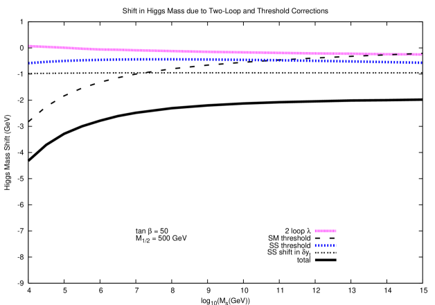
Figure 4: Same as Fig.3 except with $\tan{\beta}=50$.

References

• [1] N. Arkani-Hamed and S. Dimopoulos, JHEP 0506, 073 (2005) [arXiv:hep-th/0405159].
• [2] G. F. Giudice and A. Romanino, Nucl. Phys. B 699, 65 (2004) [Erratum-ibid. B 706, 65 (2005)] [arXiv:hep-ph/0406088].
• [3] R. Mahbubani, arXiv:hep-ph/0408096.
• [4] B. Mukhopadhyaya and S. SenGupta, Phys. Rev. D 71, 035004 (2005) [arXiv:hep-th/0407225].
• [5] A. Pierce, Phys. Rev. D 70, 075006 (2004) [arXiv:hep-ph/0406144].
• [6] A. Arvanitaki, C. Davis, P. W. Graham and J. G. Wacker, Phys. Rev. D 70, 117703 (2004) [arXiv:hep-ph/0406034].
• [7] W. Kilian, T. Plehn, P. Richardson and E. Schmidt, Eur. Phys. J. C 39, 229 (2005) [arXiv:hep-ph/0408088].
• [8] J. L. Hewett, B. Lillie, M. Masip and T. G. Rizzo, JHEP 0409, 070 (2004) [arXiv:hep-ph/0408248].
• [9] N. Arkani-Hamed, S. Dimopoulos, G. F. Giudice and A. Romanino, Nucl. Phys. B 709, 3 (2005) [arXiv:hep-ph/0409232].
• [10] L. Susskind, arXiv:hep-th/0405189.
• [11] R. Hempfling and A. H. Hoang, Phys. Lett. B 331, 99 (1994) [arXiv:hep-ph/9401219]. H. E. Haber, R. Hempfling and A. H. Hoang, Z. Phys. C 75, 539 (1997) [arXiv:hep-ph/9609331]. M. Carena, M. Quiros and C. E. M. Wagner, Nucl. Phys. B 461, 407 (1996) [arXiv:hep-ph/9508343].
• [12] A. Sirlin and R. Zucchini, Nucl. Phys. B 266, 389 (1986).
• [13] R. Hempfling and B. A. Kniehl, Phys. Rev. D 51, 1386 (1995) [arXiv:hep-ph/9408313].
• [14] A. Sirlin, Phys. Rev. D 22, 971 (1980).
• [15] S. Eidelman et al. [Particle Data Group], Phys. Lett. B 592, 1 (2004).
• [16] H. E. Haber and G. L. Kane, Phys. Rept.  117, 75 (1985).
• [17] [CDF Collaboration], arXiv:hep-ex/0507091.
• [18] N. Gray, D. J. Broadhurst, W. Grafe and K. Schilcher, Z. Phys. C 48, 673 (1990).
• [19] K. G. Chetyrkin and M. Steinhauser, Phys. Rev. Lett.  83, 4001 (1999) [arXiv:hep-ph/9907509]. Nucl. Phys. B 573, 617 (2000) [arXiv:hep-ph/9911434].
• [20] M. x. Luo and Y. Xiao, Phys. Rev. Lett.  90, 011601 (2003) [arXiv:hep-ph/0207271]. M. x. Luo, H. w. Wang and Y. Xiao, Phys. Rev. D 67, 065019 (2003) [arXiv:hep-ph/0211440].
• [21] M. E. Machacek and M. T. Vaughn, Nucl. Phys. B 222, 83 (1983). Nucl. Phys. B 236, 221 (1984). Nucl. Phys. B 249, 70 (1985).
• [22] H. Arason, D. J. Castano, B. Keszthelyi, S. Mikaelian, E. J. Piard, P. Ramond and B. D. Wright, Phys. Rev. D 46, 3945 (1992).
• [23] M. Bohm, H. Spiesberger and W. Hollik, Fortsch. Phys.  34, 687 (1986).
• [24] R. Barate et al. [LEP Working Group for Higgs boson searches], Phys. Lett. B 565, 61 (2003) [arXiv:hep-ex/0306033].