Heavy-quark production at large rapidities at hadron colliders

Abstract:

We investigate heavy-quark production as a function of the rapidity interval between two heavy quarks in hadronic collisions. We compare the results relevant to bottom production at the Tevatron and at LHC, obtained using exact leading-order and NLO pQCD production, as well as the contribution of the $4b$ channel with and without the addition of BFKL gluon radiation.

1 Introduction

One of the most important processes at high-energy hadron-hadron colliders is the production of heavy quarks. Bottom and top quark production, for example, provide not only many tests of perturbative QCD, but also some of the most important backgrounds to new physics processes. Not surprisingly, therefore, such heavy-quark production has been extensively studied in the literature (see e.g. Ref. [1] for a review) and the phenomenology at the Tevatron and the LHC has been evaluated in great detail.

In the kinematic region in which the transverse momentum of the heavy quark $Q$ is of the same order as its mass $m_{Q}$, the leading-order contribution to the inclusive heavy-quark production cross section comes from the partonic subprocesses in which a $Q\bar{Q}$ pair is produced, $gg,q\bar{q}\to Q\bar{Q}$. The next-to-leading order (NLO) corrections to these processes have been available for quite some time now [2, 3, 4, 5]. They are numerically important, particularly for $b$ quarks, where they can result in a $K$ factor as large as two.

At the parton level, these large radiative corrections to the total rates are easily identified as coming from production near threshold, $\hat{s}\sim 4m_{Q}^{2}$ ($\hat{s}$ being the partonic centre-of-mass energy squared). When folding partonic cross sections with parton distribution functions (pdfs) to get the observable rates, the threshold region is especially relevant in those cases in which the total hadronic energy $\sqrt{S}$ is of the same order as the quark mass, as for example for top production at the Tevatron, or $b$ production at fixed-target facilities. Potentially large logarithms appear in the perturbative expansion, and these need to be resummed to all orders. In practice, however, this resummation only marginally increases the NLO predictions (see e.g. Ref. [6]).

Total partonic rates can also receive large contributions from the high-energy region $\hat{s}\gg 4m_{Q}^{2}$, complementary to the threshold region. As discussed in Ref. [2], this is due to those partonic subprocesses that feature a gluon exchange in the $t$-channel; this happens for $gg\to Q\bar{Q}g$ and $qg\to Q\bar{Q}q$, and it is peculiar to the NLO computations of quark pair production, as opposed to Born-level predictions, in which only fermions are exchanged in the $t$ channel. It must be stressed that at the hadron level this enhancement is diluted by the fall-off of the pdfs at large $x$ values [7, 8].

A gluon exchange in the $t$-channel is also present at ${\cal O}(\alpha_{\scriptscriptstyle S}^{4})$ in the reaction $gg\to Q\bar{Q}Q\bar{Q}$, which is the Born-level contribution to this four-quark process. This is interesting, since the $t$-channel gluon exchange leads to properties fairly similar to those relevant to the Mueller-Navelet dijet cross section [9], which is used to study the high-energy limit of QCD in which the energy dependence of the lowest-order cross section is enhanced by BFKL-type logarithmic corrections [10, 11, 12].

The dominance of the gluon exchange in the $t$-channel implies that the $4Q$ channel is perturbatively suppressed only by a factor of $\alpha_{\scriptscriptstyle S}$ with respect to pair production at high energies. Although this still prevents us from a straightforward use of $4Q$ production to detect BFKL signals, we can, however, observe that in the high-energy regime the kinematics of the $2Q$ and $4Q$ production channels are rather different. The former is dominated by those configurations in which the $Q\bar{Q}$ pair recoils with large rapidity against a fast light parton. On the other hand, the $4Q$ system will predominantly be produced in two $Q\bar{Q}$ pairs, rapidly moving away from each other; the relative rapidity of each pair is small compared to the separation in rapidity of the two pairs. Therefore by selecting particular kinematic configurations it may be possible to relatively enhance the $4Q$ contribution and find signatures of BFKL. This is the main focus of our study.

In order to define a proper set of observables, we require for each event to tag (at least) two heavy flavours (in any possible combination: $Q\bar{Q}$, $QQ$, or $\bar{Q}\bar{Q}$), which we denote by $Q_{1}$ and $Q_{2}$, separated by a large rapidity interval, $\Delta y=|y_{Q_{1}}-y_{Q_{2}}|\gg 1$. In this way, we should cut off the configurations that dominate pair production in the high-energy regime, without losing too many events in the $4Q$ channel. We aim at studying whether this is the case or not, specifically in the regions accessible to the detectors at present and future colliders, by comparing the predictions for $2Q$ and $4Q$ production processes. We stress that our set of observables is based on a double $Q$ tagging, which in fact is already used to study $Q\bar{Q}$ correlations in heavy-quark pair production. In this paper, we shall not correct our results for tagging efficiency.

The high-energy limit of $4Q$ production can be considered as a reformulation of the standard Mueller-Navelet dijet case. What we are doing here, in effect, is replacing each Mueller-Navelet forward jet (with $p_{T}>P_{T{\rm min}}$) by a $Q\bar{Q}$ pair. In fact, by identifying the rapidity of each pair with the rapidity of the tagged quark in the pair, we have $\hat{s}=4m_{Q_{\perp}}^{2}\cosh^{2}y^{*}$, where $m_{Q_{\perp}}^{2}={p^{2}_{Q_{\perp}}+m_{Q}^{2}}$ is the squared heavy-quark transverse mass, and $y^{*}=(\Delta y)/2$. The formula above, relating the large-$\hat{s}$ to the large-$y^{*}$ region, is customary in Mueller-Navelet arguments. The differences between jet and heavy-quark production are easy to find: whereas in the dijet case it is $P_{T{\rm min}}$ that regulates the infrared singularities at $\hat{t}=0$, here it is the heavy-quark mass $m_{Q}$. The analogue of the $P_{T{\rm min}}^{2}\hat{\sigma}_{jj}\to\$constant behaviour of the leading-order dijet cross section at large dijet rapidity separation $\Delta y$ is the $m_{Q}^{2}\hat{\sigma}_{4Q}\to\$constant behaviour of the $4Q$ heavy-quark cross section. The effect of the (leading logarithm) BFKL corrections is the same in both cases: the partonic cross sections increase asymptotically as $\exp(\lambda\Delta y)$ where $\lambda=4\log{2}N_{c}\alpha_{\scriptscriptstyle S}/\pi$ and $\Delta y$ is either the rapidity separation of the dijets in the Mueller-Navelet case, or the rapidity separation of the two $Q\bar{Q}$ systems in the present context.

Another process of potential interest in the high-energy limit is $Q\bar{Q}+1$ jet production. In this case the partonic subprocesses $gg\to Q\bar{Q}g$ and $qg\to Q\bar{Q}q$, which feature a gluon exchange in the $t$-channel, are ${\cal O}(\alpha_{\scriptscriptstyle S}^{3})$ at the Born level. This can also be considered as a reformulation of the standard Mueller-Navelet analysis, where only one of the forward jets is replaced by a $Q\bar{Q}$ pair.

This paper is organized as follows. In Section 2 we compute analytically the high-energy limit of the $gg\to Q\bar{Q}Q\bar{Q}$ cross section. In Section 3, we describe how to include the resummation of BFKL logarithms, through Monte Carlo methods. In Section 4, results for $2Q$ and $4Q$ channels are compared, at the Tevatron and LHC energies. We also consider the case of $Q\bar{Q}+1$ jet production. Finally, in Section 5 we present our conclusions. The appendices collect some useful formulae.

2 The high-energy limit

In the high-energy limit, the $\Delta y$ distribution for $Q\bar{Q}$ production can be written schematically as

$$\frac{d\sigma_{Q\bar{Q}}}{\Delta y}\,\sim\,\alpha_{\scriptscriptstyle S}^{2}\sum_{j=0}^{\infty}a_{0j}\alpha_{\scriptscriptstyle S}^{j}\ +\ \alpha_{\scriptscriptstyle S}^{4}\sum_{j=0}^{\infty}a_{1j}(\alpha_{\scriptscriptstyle S}L)^{j}\ +\ \alpha_{\scriptscriptstyle S}^{4}\sum_{j=0}^{\infty}a_{2j}\alpha_{\scriptscriptstyle S}(\alpha_{\scriptscriptstyle S}L)^{j}\ +\cdots,$$ (1)

where $L=\log(\hat{s}/\mu_{\scriptscriptstyle\rm W}^{2})\simeq\Delta y$ is a large logarithm, and the quantity $\mu_{\scriptscriptstyle\rm W}^{2}$ is a mass scale squared, typically of the order of the crossed-channel momentum transfer and/or of the heavy-quark masses. The first sum in Eq. (1) is a fixed-order expansion in $\alpha_{\scriptscriptstyle S}$ starting at ${\cal O}(\alpha_{\scriptscriptstyle S}^{2})$ (the Born processes $q\bar{q},gg\to Q\bar{Q}$), which collects together the contributions that do not feature gluon exchange in the crossed channel between the heavy quarks.

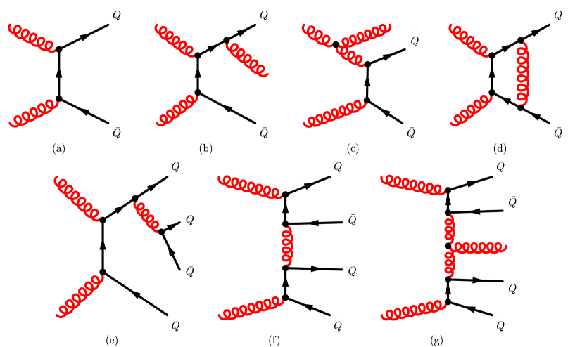
Figure 1: Amplitudes for $Q\bar{Q}$ production in $gg$ fusion. Figure (a) represents the leading-order term. Figures (b), (c) and (d) are examples of the diagrams that contribute to the NLO term. Figures (e) and (f) represent the 4 $Q$ contribution to the NNLO term; figure (e) ((f)) is an example of a diagram with quark (gluon) exchange in the $t$ channel. Figure (f) constitutes also the leading term of a BFKL gluon ladder, and figure (g) represents the first rung of it.

The $a_{00}$ coefficient is the leading-order term, which for $gg$ fusion is depicted in Fig. 1(a); the $a_{01}$ coefficient is the NLO term (specimen diagrams are given in Fig. 1(b-d)). An example of a $4Q$ contribution to the $a_{02}$ coefficient is given in Fig. 1(e). The $a_{0j}$ coefficients behave like $1/\hat{s}$, or equivalently $\exp(-\Delta y)$, modulo logarithmic corrections. In Eq. (1), the second and third sums collect the contributions which feature only gluon exchange in the crossed channel between heavy quarks, the second (third) sum resumming the BFKL (next-to-)leading logarithmic corrections. Fig. 1(f) represents the zeroth-order term, and Fig. 1(g) contributes to the first-order term, of the second sum. The $a_{1j}$ and $a_{2j}$ coefficients behave like $1/\mu_{\scriptscriptstyle\rm W}^{2}$, in contrast to the $1/\hat{s}$ behaviour of the $a_{0j}$. The ellipses of Eq. (1) refer to logarithmic corrections beyond the next-to-leading accuracy. Thus, it is clear that the second and third sums of Eq. (1) will eventually dominate over the first sum in the asymptotic energy region $\hat{s}\to\infty$. In Sections 2 and 3 we will analyse the second sum of Eq. (1) in the region $\hat{s}\gg\mu_{\scriptscriptstyle\rm W}^{2}$, by computing the $a_{1j}$ coefficients in the high-energy limit.

Details of the calculation for the production of four heavy quarks, via the sub-processes $gg\to Q\bar{Q}Q\bar{Q}$ and $q\bar{q}\to Q\bar{Q}Q\bar{Q}$, are presented in Appendix A. In the high-energy limit, we require that any two $Q$’s (no distinction between $Q$ and $\bar{Q}$ is necessary) are produced at large rapidity separation. Then the production process is dominated by the sub-processes for which the tagged $Q$’s are separated by gluon exchange in the crossed channel. Of the above two sub-processes, only $gg\to Q\bar{Q}Q\bar{Q}$ features gluon exchange in the crossed channel. With the kinematics of the high-energy limit,

$$y_{Q_{1}}\simeq y_{\bar{Q}_{2}}\gg y_{Q_{3}}\simeq y_{\bar{Q}_{4}}\,,\qquad p_{Q_{1\perp}}\simeq p_{\bar{Q}_{2\perp}}\simeq p_{Q_{3\perp}}\simeq p_{\bar{Q}_{4\perp}}\,,$$ (2)

the amplitude for $gg\to Q\bar{Q}Q\bar{Q}$ factorises as

$$|{\cal M}_{g_{a}g_{b}\to Q_{1}\bar{Q}_{2}Q_{3}\bar{Q}_{4}}|^{2}=\frac{4\hat{s}^{2}}{\hat{t}^{2}}\left[I^{Q\bar{Q}}(p_{a},p_{Q_{f}},p_{{\bar{Q}}_{f}};q)I^{Q\bar{Q}}(p_{b},p_{Q_{b}},p_{{\bar{Q}}_{b}};-q)\right]\,,$$ (3)

where $Q_{f}(\bar{Q}_{f})$ and $Q_{b}(\bar{Q}_{b})$ are the quarks (anti-quarks) produced forward and backward, respectively. In Eq. (3),

$$\hat{t}=q^{2}=(p_{a}-p_{Q_{f}}-p_{\bar{Q}_{f}})^{2}$$ (4)

is the momentum transfer. The impact factor $I^{Q\bar{Q}}$ is calculated in Appendix B, starting from the amplitude for $g\,i\to Q\bar{Q}i$ with $i=q,g$ and using high-energy factorisation. The result is given in Eq. (29), summed (averaged) over final (initial) colours and helicities. In the kinematics of (2), the exact parton momentum fractions (25) are well approximated by

$$x_{a}^{0}={m_{Q_{1\perp}}e^{y_{Q_{1}}}+m_{\bar{Q}_{2\perp}}e^{y_{\bar{Q}_{2}}}\over\sqrt{S}}\;,\qquad x_{b}^{0}={m_{Q_{3\perp}}e^{-y_{Q_{3}}}+m_{\bar{Q}_{4\perp}}e^{-y_{\bar{Q}_{4}}}\over\sqrt{S}}\,.$$ (5)

Using Eq. (3), we can write the cross section for heavy-quark production as

$${d\sigma\over\prod_{i=1}^{4}d^{2}{\bf p}_{Q_{i\perp}}dy_{Q_{i}}}$$ (6)

$$= x_{a}^{0}g_{a/A}(x_{a}^{0},\mu_{{\scriptscriptstyle F}a}^{2})\,x_{b}^{0}g_{b/B}(x_{b}^{0},\mu_{{\scriptscriptstyle F}b}^{2})\ {I^{Q\bar{Q}}(q_{a})I^{Q\bar{Q}}(q_{b})\over 2\pi^{4}(4\pi)^{4}q_{a_{\perp}}^{2}q_{b_{\perp}}^{2}}\,{\delta^{2}({\bf q}_{a_{\perp}}-{\bf q}_{b_{\perp}})\over 2}\,,$$

with momentum transfers $q_{a}=p_{a}-p_{Q_{1}}-p_{\bar{Q}_{2}}$ and $q_{b}=p_{Q_{3}}+p_{\bar{Q}_{4}}-p_{b}$, and where $g_{a/A}(x_{a}^{0},\mu_{{\scriptscriptstyle F}a}^{2})$ is the pdf for the gluon $g_{a}$, and analogously for $g_{b}$. We use the notation $\mathbf{p}_{\perp}$ to denote a transverse momentum vector.

However, in Eq. (6) energy and longitudinal momentum are not conserved. The parton momentum fractions in the high-energy limit, $x_{a}^{0}$ and $x_{b}^{0}$, underestimate the exact ones, $x_{a}$ and $x_{b}$, Eq. (25) and accordingly the values of the pdfs are overestimated. Thus for the numerical applications of Section 4 we will use the factorised form (6) of the production rate, but with $x_{a}^{0}\to x_{a}$ and $x_{b}^{0}\to x_{b}$. This modification is particularly important when BFKL evolution is considered.

The above results must be integrated over the phase space of the final-state particles in order to get physical results. In the high-energy limit, the phase space (21) can be factorised into the phase spaces for the two impact factors,

$$d{\cal P}_{4} = \left(\prod_{i=1,2}{d^{3}p_{Q_{i}}\over(2\pi)^{3}2p^{0}_{Q_{i}}}\,2\pi\,\delta(p_{a}^{+}-p_{Q_{1}}^{+}-p_{\bar{Q}_{2}}^{+})\right)\,\left(\prod_{i=3,4}{d^{3}p_{Q_{i}}\over(2\pi)^{3}2p^{0}_{Q_{i}}}\,2\pi\,\delta(p_{b}^{-}-p_{Q_{3}}^{-}-p_{\bar{Q}_{4}}^{-})\right)$$ (7)

$$\times(2\pi)^{2}\,\delta^{2}({\bf p}_{Q_{1\perp}}+{\bf p}_{\bar{Q}_{2\perp}}+{\bf p}_{Q_{3\perp}}+{\bf p}_{\bar{Q}_{4\perp}})\,,$$

where we have used light-cone coordinates $p^{\pm}=(p^{0}\pm p^{3})/\sqrt{2}$. Fixing

$$z_{a}={p_{Q_{1}}^{+}\over p^{+}_{Q_{1}}+p_{\bar{Q}_{2}}^{+}}\,,\qquad z_{b}={p_{Q_{3}}^{-}\over p^{-}_{Q_{3}}+p_{\bar{Q}_{4}}^{-}}\,,$$ (8)

the phase space (7) can be rewritten as

$$d{\cal P}_{4} = {1\over(4\pi)^{2}}{1\over 2\hat{s}}\left({dz_{a}\over z_{a}(1-z_{a})}{d^{2}{\bf p}_{Q_{1\perp}}\over(2\pi)^{2}}\right)\left({dz_{b}\over z_{b}(1-z_{b})}{d^{2}{\bf p}_{Q_{3\perp}}\over(2\pi)^{2}}\right)$$ (9)

$$\times{d^{2}{\bf q}_{a_{\perp}}\over(2\pi)^{2}}{d^{2}{\bf q}_{b_{\perp}}\over(2\pi)^{2}}(2\pi)^{2}\,\delta^{2}({\bf q}_{a_{\perp}}-{\bf q}_{b_{\perp}})\,,$$

with centre-of-mass energy $\hat{s}=2p_{a}^{+}p_{b}^{-}$. Note that Eq. (9) is written in such a way as to be immediately generalizible to the emission of a BFKL gluon ladder between the impact factors.

Using Eqs. (3) and (9) in the expression for the cross section given in (20), we obtain

$$d{\hat{\sigma}}(p_{a}p_{b}\to p_{Q_{1}},p_{\bar{Q}_{2}}p_{Q_{3}}p_{\bar{Q}_{4}})={d^{2}{\bf q}_{a_{\perp}}\over(2\pi)^{2}}{d^{2}{\bf q}_{b_{\perp}}\over(2\pi)^{2}}{{\cal I}({\bf q}_{a_{\perp}})\over q_{a_{\perp}}^{2}}{{\cal I}({\bf q}_{b_{\perp}})\over q_{b_{\perp}}^{2}}(2\pi)^{2}\,\delta^{2}({\bf q}_{a_{\perp}}-{\bf q}_{b_{\perp}})\,,$$ (10)

where the integrated impact factor is

$${\cal I}({\bf q_{\perp}})={1\over 4\pi}\int_{0}^{1}{dx\over x(1-x)}{d^{2}{\bf p_{\perp}}\over(2\pi)^{2}}I^{Q\bar{Q}}(x,{\bf p_{\perp}};{\bf q_{\perp}})\,,$$ (11)

with $I^{Q\bar{Q}}$ given in Eq. (29). The integral is explicitly performed in Section B.1, where it is expressed in terms of a function $g$, Eq. (B.1), of the dimensionless ratio $\xi=q_{\perp}^{2}/m_{Q}^{2}$. Then using Eqs. (35)-(B.1), the total integrated cross section (10) becomes

$$\sigma_{gg}=\frac{\alpha_{\scriptscriptstyle S}^{4}}{m_{Q}^{2}}\frac{N_{c}^{2}-1}{4\pi}\int_{0}^{\infty}\;\frac{d\xi_{a}}{\xi_{a}}\;\frac{d\xi_{b}}{\xi_{b}}\;g(\xi_{a})g(\xi_{b})\delta(\xi_{a}-\xi_{b})\,.$$ (12)

Note that even though according to Eq. (38) the function $g(\xi)$ grows logarithmically with $\xi$ as $\xi\to\infty$, the integral in (12) is finite and gives [13]

$$\sigma_{gg} = \frac{\alpha_{\scriptscriptstyle S}^{4}}{\pi m_{Q}^{2}}\frac{1}{N_{c}^{2}-1}\left[{23N_{c}^{2}\over 81}-{277\over 486}+\left({175\zeta(3)\over 576}-{19\over 288}\right){1\over N_{c}^{2}}\right]$$ (13)

$$\approx \frac{\alpha_{\scriptscriptstyle S}^{4}}{m_{Q}^{2}}\;0.0803\,.$$

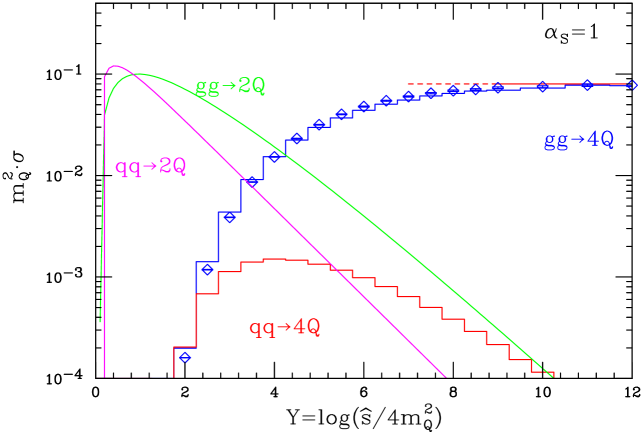
Figure 2: Partonic cross section for $Q\bar{Q}$ and $Q\bar{Q}Q\bar{Q}$ production. The histograms show the exact leading-order results, i.e., the exact matrix elements integrated over the exact phase space. The diamonds are obtained integrating the high-energy limit of the matrix element, Eq. (3), with the exact phase space. The patterned red line is Eq. (13), representing the asymptotic limit. For comparison, the Born $gg,q\bar{q}\to Q\bar{Q}$ contributions are also shown. The coupling $\alpha_{\scriptscriptstyle S}$ is set to one. Note that the kinematic limit for $b$-quark production at the Tevatron is at $Y\approx 10.6$.

The results obtained in this section are summarized in Fig. 2. The exact leading-order results for the $gg\to Q\bar{Q}Q\bar{Q}$ and $q\bar{q}\to Q\bar{Q}Q\bar{Q}$ processes, obtained with MADGRAPH/MADEVENT [14, 15], are shown (histograms) as a function of $Y=\log(\hat{s}/4m_{Q}^{2})$. The dominance of the $t$-channel gluon exchange contribution, present only in the case of $gg$ initial state, is apparent. The diamonds are obtained by integrating the high-energy limit of the matrix element, Eq. (3), with the exact phase space; the difference with the exact result is fairly small, which implies that, at the dynamical level, the high-energy limit is a good approximation. The approximation of the phase space is evidently more drastic, and results in the constant (dashed) red line, whose value is taken from Eq. (13). For comparison we also show the Born $gg,q\bar{q}\to Q\bar{Q}$ processes corresponding to the $a_{00}$ contribution in Eq. (1). As argued above, and in contrast to the $gg\to Q\bar{Q}Q\bar{Q}$ contribution, these exhibit a $\exp(-Y)$ behaviour in the high-energy (large $Y$) limit.

3 The BFKL Monte Carlo

As we have seen, in the high-energy limit (2) the cross section for the production of four heavy quarks is dominated by processes with a gluon exchange in the crossed channel. In that limit, the BFKL formalism resums the universal leading-logarithmic (LL) corrections, of ${\cal O}(\alpha_{\scriptscriptstyle S}^{n}\log^{n}(\hat{s}/|\hat{t}|))$, with $\hat{t}$ defined in Eq. (4). These are obtained in the limit of strong rapidity ordering of the emitted gluon radiation,

$$y_{Q_{1}}\simeq y_{\bar{Q}_{2}}\gg y_{1}\gg y_{2}\gg\ldots\gg y_{n-1}\gg y_{n}\gg y_{Q_{3}}\simeq y_{\bar{Q}_{4}}\,,$$ (14)

where we label by $1,\ldots,n$ the emission of $n$ gluons along the BFKL ladder. Because of the strong rapidity ordering, the contribution of the gluons to the parton momentum fractions (5) is subleading, and it is therefore neglected to LL accuracy. The BFKL-resummed cross section for the production of four heavy quarks is then given by Eq. (6), where the $\delta$ function, $\delta^{2}({\bf q}_{a_{\perp}}-{\bf q}_{b_{\perp}})/2$, is replaced by the solution of the BFKL equation,

$$f({\bf q}_{a_{\perp}},{\bf q}_{b_{\perp}},\Delta y)\,={1\over(2\pi)^{2}\sqrt{q_{a_{\perp}}^{2}q_{b_{\perp}}^{2}}}\sum_{n=-\infty}^{\infty}e^{in\phi}\,\int_{-\infty}^{\infty}d\nu\,e^{\omega(\nu,n)\Delta y}\,\left(q_{a_{\perp}}^{2}\over q_{b_{\perp}}^{2}\right)^{i\nu}\,,$$ (15)

with $\phi$ the azimuthal angle between $q_{a}$ and $q_{b}$, and $\omega(\nu,n)$ the eigenvalue of the BFKL equation with maximum at $\omega(0,0)=4\log{2}C_{A}\alpha_{\scriptscriptstyle S}/\pi$. Thus the solution of the BFKL equation resums powers of $\Delta y$, and rises with $\Delta y$ as $f({\bf q}_{a_{\perp}},{\bf q}_{b_{\perp}},\Delta y)\sim\exp(\omega(0,0)\Delta y)$.

However, in a comparison with experimental data, it must be remembered that the LL BFKL resummation makes some approximations which, even though formally subleading, can be numerically important: $a)$ the BFKL resummation is performed at fixed coupling constant, and thus any variation in the scale at which $\alpha_{\scriptscriptstyle S}$ is evaluated appears in the next-to-leading-logarithmic (NLL) terms; $b)$ because of the strong rapidity ordering any two-parton invariant mass is large. Thus there are no collinear divergences in the LL resummation in the BFKL ladder; $c)$ finally, energy and longitudinal momentum are not conserved, since the momentum fractions $x$ of the incoming partons are reconstructed from the kinematic variables of the four heavy quarks only, without including the radiation from the BFKL ladder. Therefore, the BFKL theory will severely underestimate the correct value of the $x$’s, and thus grossly overestimate the gluon luminosities. In fact, if four heavy quarks $+\ n$ gluons are produced, the correct evaluation of the $x$’s yields

$$x_{a}=\sum_{i=1}^{4}{m_{Q_{i\perp}}e^{y_{Q_{i}}}\over\sqrt{S}}+\ \sum_{j=1}^{n}{p_{j\perp}e^{y_{i}}\over\sqrt{S}}\qquad x_{b}=\sum_{i=1}^{4}{m_{Q_{i\perp}}e^{-y_{Q_{i}}}\over\sqrt{S}}+\ \sum_{j=1}^{n}{p_{j\perp}e^{-y_{i}}\over\sqrt{S}}\,,$$ (16)

where $p_{j\perp}$ are the transverse momenta of the gluons produced along the BFKL ladder.

In the standard (analytic) approach to BFKL, which leads to Eq. (15), it is not possible to take the contribution of the BFKL gluon radiation into account in Eq. (16). This is because in deriving Eq. (15) one has already integrated over the full rapidity ordered phase space for BFKL gluon radiation. To gain information on the BFKL gluon momenta we need to unfold the gluon integrations. This approach results in an explicit sum over the number of emitted BFKL gluons, where each term in the sum is an integral over the rapidity ordered BFKL gluon phase space. The solution to the BFKL equation can then be obtained (numerically) while maintaining information about each emitted gluon by evaluating these integrals in a Monte Carlo approach [16, 17]. Besides allowing energy and momentum conservation to be observed by including the BFKL gluon contribution to Eq. (16), this approach also allows subleading effects originating from the running of the coupling to be taken into account. The method has recently been generalised to solve the BFKL equation at full NLL accuracy [18, 19], although some work remains to be done before it can be applied in a phenomenological study like the one presented here.

The Monte Carlo formulation of Ref. [17] is, in its simplest form, applicable only when the transverse momentum of at least one end of the BFKL chain is kept bigger than some cut-off $|\mathbf{q}_{i}|>P_{\perp}\gg\mu$ with $i\in\{a,b\}$, and $\mu$ the resolution scale of the BFKL Monte Carlo (see Ref. [17] for further details). It was demonstrated in Ref. [17] that in the case of hadronic dijet production with a minimum $P_{\perp}=20$ GeV, the residual $\mu$-dependence is negligible for $\mu\leq 6$ GeV. Varying $\mu$ will shift contributions between different $f^{(n)}$’s describing the contribution from different numbers of resolved gluons.

However, in the current process of $4Q$ production there is no minimum transverse momentum scale at either end of the BFKL chain. To resolve the problem thus faced by the BFKL MC formulation we cut out a small region of phase space corresponding to $p_{\perp}<0.05$ GeV at one end of the chain. The contribution from this very small region of phase space is negligible, but nevertheless this cut-off is sufficient to permit the use of the unfolded BFKL formalism. In principle $\mu$ could then be chosen arbitrarily small compared to the cut-off, but this would result in very slow convergence due to the extremely large number of resolved gluons with a transverse momentum above this scale. Instead, $\mu$ is chosen according to the transverse momentum at one end of the BFKL chain in 5 steps. This keeps the average number of resolved gluons under control and thus ensures rapid convergence, while maintaining the very weak $\mu$-dependence of the overall result.

In order to demonstrate the behaviour of the BFKL ladder, we consider the production of four heavy quarks assuming that all of them are detected. We study the production rate as a function of the transverse momentum ${\bf q}_{a_{\perp}}=-{\bf p}_{Q_{1\perp}}-{\bf p}_{\bar{Q}_{2\perp}}$ exiting from the impact factor $I^{Q\bar{Q}}(q_{a})$. At leading order, the transverse momenta of the two pairs are equal, ${\bf q}_{a_{\perp}}={\bf q}_{b_{\perp}}={\bf q}_{{}_{\perp}}$. Since we know from Eqs. (38) and (B.1) that the scaling of the integrated impact factor is $g(\xi)\sim{\cal O}(\xi)$, with $\xi=q_{\perp}^{2}/m_{Q}^{2}$, power counting from Eq. (12) shows that at leading order $d\sigma/dq_{{}_{\perp}}\sim{\cal O}(q_{{}_{\perp}})$ as $q_{{}_{\perp}}\to 0$. When the BFKL gluon radiation is included, the production rate is hardened in the infrared and we obtain

$${d\sigma\over dq_{a_{\perp}}dq_{b_{\perp}}}\sim{\rm const.}\qquad{\rm as}\qquad q_{a_{\perp}}\to 0\ ,\quad q_{b_{\perp}}\to 0\,.$$ (17)

In Fig. 3 we plot the transverse momentum distribution $d\sigma/dq_{a_{\perp}}dq_{b_{\perp}}$ evaluated at $q_{a_{\perp}}=q_{b_{\perp}}=p_{\perp}$. The solid red curve is the four-quark production (6), but with the high-energy parton momentum fractions replaced by the exact ones, $x_{a}^{0}\to x_{a}$ and $x_{b}^{0}\to x_{b}$; in this case, the two impact factors have equal transverse momenta ${\bf q}_{a_{\perp}}={\bf q}_{b_{\perp}}$. The dashed blue curve corresponds to the high-energy limit of leading-order four-quark production (6) with the BFKL ladder included. In this case ${\bf q}_{a_{\perp}}$ is no longer restricted to be equal to ${\bf q}_{b_{\perp}}$, which explains why the BFKL curve is lower than the leading-order one. However, we see that the spectrum is relatively harder for $p_{\perp}\to 0$ in the BFKL case.

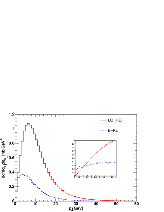
Figure 3: The transverse momentum distribution $d\sigma/dq_{a_{\perp}}dq_{b_{\perp}}$ evaluated at $dq_{b_{\perp}}\!=\!dq_{b_{\perp}}\!=\!p_{\perp}$. The solid red curve corresponds to the high-energy limit of leading-order four $b$-quark production, with $m_{b}=5$ GeV. The dashed blue curve corresponds to adding BFKL evolution to the gluon exchanged in the $t$-channel.

4 BFKL signals at the Tevatron and LHC

4.1 Inclusive heavy-quark production

In this section we compare the results for the $4Q$ channel, obtained with the BFKL MC described in the previous section, with those relevant to $Q\bar{Q}$ production, obtained with the NLO code of Ref. [5] and MC@NLO [20, 21]. We consider bottom quark production, with $m_{b}=5$ GeV, since $b$-quarks are readily identifiable at the Tevatron and LHC. In the case of pair production, we need to use a NLO computation in order to explicitly verify that, with our chosen set of cuts, large non-BFKL logarithms do not appear in the cross section, which is a necessary condition in order to study BFKL signals with the $4Q$ channel.

Figure 4 shows the integrated cross section

$$\sigma(\Delta y)=\int_{\Delta y}^{\infty}d\Delta y^{\prime}\frac{d\sigma}{d\Delta y}(\Delta y^{\prime})$$ (18)

as a function of $\Delta y$, the rapidity distance between the two tagged quarks (which, for this process, are $b$ and $\bar{b}$), at Tevatron and at LHC energies. In order to simulate a realistic detector coverage, the rapidity of both quarks is required to be less than 2.5, and therefore $\Delta y=5$ is the largest accessible rapidity separation. We also consider additional cuts on the transverse momenta of the tagged quarks, imposing $p_{{\rm T}b,\bar{b}}>5$ and 10 GeV. The two-loop running of the strong coupling $\alpha_{\scriptscriptstyle S}$, and the MRST99 package [22] of pdfs has been used, with factorisation scale set to $\mu_{\scriptscriptstyle F}^{2}=(m_{b_{\perp}}^{2}+m_{\bar{b}_{\perp}}^{2})/2$.

Figure 4: Integrated cross sections as a function of $\Delta y$, at LO (dashed histograms) and NLO (solid histograms), with no cut on the transverse momentum $p_{\rm T}$, and with $p_{\rm T}>5$ and 10 GeV, at the Tevatron (left panel) and LHC (right panel) energies. The code of Ref. [5] has been used.

¿From the figure we can see that the cuts on the transverse momenta largely reduce the impact of radiative corrections. However, this information alone is not sufficient to guarantee that non-BFKL logs do not spoil the perturbative expansion. In order to investigate this issue, we thus recomputed the cross section with MC@NLO [20, 21], which, by matching the NLO results with the HERWIG [23] parton shower, improves the fixed-order result by effectively resumming various classes of large logs. In the case in which no $p_{\rm T}$ cuts are applied, the MC@NLO results are basically coincident with the NLO ones. However, by imposing $p_{{\rm T}b,\bar{b}}>5$ GeV, the MC@NLO cross section is roughly a factor 1.7 larger than the NLO, in the whole $\Delta y$ range considered. This is due to the fact that the $p_{\rm T}$ cuts render the cross section sensitive to Sudakov effects. Although these could be reduced by imposing different $p_{\rm T}$ cuts on the two tagged $b$’s, it is quite problematic to eliminate them completely. Thus, the pure NLO result must be regarded, at least for the $p_{\rm T}$ cuts considered here, as a lower bound on the $b\bar{b}$ inclusive cross section.

In order to be definite, we require $p_{{\rm T}b,\bar{b}}>5$ GeV in what follows. In Fig. 5, we plot the integrated cross section for $b\bar{b}$ production as a function of $\Delta y$, at Tevatron and at LHC energies. For the sake of comparison, we display again here the middle NLO curves of Fig. 4. In addition, the dot-dashed red curve displays the high-energy limit contribution of the $4Q$ channel to inclusive $2Q$ production, where $Q=b$ or $\bar{b}$. The factorisation and renormalisation scales have been set to $\mu_{{\scriptscriptstyle F}a}^{2}=\mu_{{\scriptscriptstyle R}a}^{2}=(m_{b_{1\perp}}^{2}+m_{\bar{b}_{2\perp}}^{2})/2$ and $\mu_{{\scriptscriptstyle F}b}^{2}=\mu_{{\scriptscriptstyle R}b}^{2}=(m_{b_{3\perp}}^{2}+m_{\bar{b}_{4\perp}}^{2})/2$. Thus, the strong coupling $\alpha_{\scriptscriptstyle S}^{4}$ must be understood here as $\alpha_{\scriptscriptstyle S}^{2}(\mu_{{\scriptscriptstyle R}a}^{2})\,\alpha_{\scriptscriptstyle S}^{2}(\mu_{{\scriptscriptstyle R}b}^{2})$, with $\alpha_{\scriptscriptstyle S}$ evolved at two loops, in accordance with the NLO calculation. The dashed blue curve is the same as the red curve but with the addition of BFKL gluon radiation. In the BFKL gluon emission chain, the value of $\alpha_{\scriptscriptstyle S}$ is taken at the $b$ mass.

Fig. 5 is the central result of this study. It shows that within the rapidity range for heavy-quark production accessible to LHC (assumed here to correspond to $\Delta y<5$) the $4Q$ channel, even augmented by the BFKL gluon radiation, can never overcome the $2Q$ channel. Thus, it cannot readily be used as a footprint of BFKL radiation.

The situation could be improved either by imposing the additional requirement that the two tagged $b$-quarks have the same sign, i.e. $bb$ or $\bar{b}\bar{b}$, or by requiring three or more $b$-quarks to be identified. In the former case, this would reduce the “$4Q$” curves in Fig. 5 by a (combinatoric) factor of two, while almost completely removing the $2b$ contribution. A realistic assessment of how much of the BFKL signal would remain in these cases would depend on the efficiencies of multi-$b$-quark tagging and charge identification (via the sign of the lepton in semi-leptonic $B$-meson decay, for example), which goes beyond the scope of the present study. Another issue that needs to be addressed by a more realistic study is the contamination from overlapping events, see for example Ref. [24].

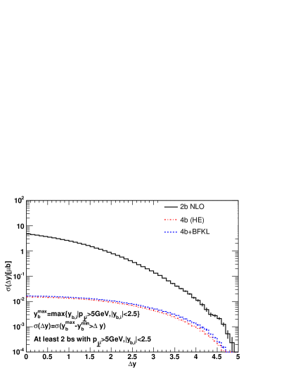
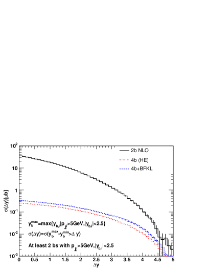
Figure 5: Integrated cross sections as a function of $\Delta y$, with $p_{\rm T}>5$ GeV, at Tevatron (left panel) and LHC (right panel) energies. The NLO curves are the same as the middle NLO curves of Fig. 4, and are displayed here for the sake of comparison. The dot-dashed red curves are the high-energy limit contributions of the $4Q$ channel to inclusive $2Q$ production; the dashed blue curves are the same as the red curves with the addition of BFKL gluon radiation.

4.2 Inclusive heavy-quark $+$ 1 jet production

As mentioned in the Introduction and in Section 2, inclusive $Q\bar{Q}+1$ jet production is also of interest in the high-energy limit, and is in a sense a hybrid of the original Mueller-Navelet 2 jet and our $4Q$ processes. In this process, a gluon is exchanged in the $t$-channel between the jet and the $Q\bar{Q}$ pair already at leading-order, which in this case is ${\cal O}(\alpha_{\scriptscriptstyle S}^{3})$. In fact, as in Eq. (1), the $\Delta y$ distribution for $Q\bar{Q}+1$ jet production in the high-energy limit can be written schematically as

$$\frac{d\sigma_{Q\bar{Q}jet}}{\Delta y}\,\sim\,\alpha_{\scriptscriptstyle S}^{3}\sum_{j=0}^{\infty}b_{0j}\alpha_{\scriptscriptstyle S}^{j}\ +\ \alpha_{\scriptscriptstyle S}^{3}\sum_{j=0}^{\infty}b_{1j}(\alpha_{\scriptscriptstyle S}L)^{j}\ +\ \alpha_{\scriptscriptstyle S}^{3}\sum_{j=0}^{\infty}b_{2j}\alpha_{\scriptscriptstyle S}(\alpha_{\scriptscriptstyle S}L)^{j}\ +\cdots,$$ (19)

where $L=\log(\hat{s}/\mu_{\scriptscriptstyle\rm W}^{2})\simeq\Delta y$ is a large logarithm, and the quantity $\mu_{\scriptscriptstyle\rm W}^{2}$ is a mass scale squared. The first sum in Eq. (19) is a fixed-order expansion in $\alpha_{\scriptscriptstyle S}$ starting at ${\cal O}(\alpha_{\scriptscriptstyle S}^{3})$, and collects the contributions which do not feature gluon exchange between the jet and the $Q\bar{Q}$ pair. The $b_{00}$ coefficient is the leading-order term (a specimen diagram is depicted in Fig. 1(b)). The second and third sums of Eq. (19) collect the contributions which feature only gluon exchange in the crossed channel between the jet and the $Q\bar{Q}$ pair, the second (third) sum resumming the BFKL (next-to-) leading logarithmic corrections. Fig. 1(c) represents the zeroth-order term of the second sum. The $b_{1j}$ and $b_{2j}$ coefficients behave like $1/\mu_{\scriptscriptstyle\rm W}^{2}$. We note, however, that in contrast to Eq. (1), the second and third sums of Eq. (19) start at the same order in $\alpha_{\scriptscriptstyle S}$ as the first sum. Thus one would expect that the onset of the dominance of the asymptotic energy region $\hat{s}\to\infty$ occurs more quickly in this case than in heavy two-quark production. We analyse this issue by computing the coefficients $b_{00}$ and $b_{1j}$.

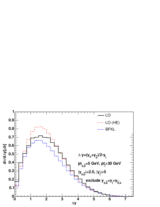
Figure 6: Inclusive heavy two-quark $+1$ jet production as a function of the rapidity separation of the jet from the average position of the heavy two-quark pair, $\Delta y=|y_{j}-(y_{b}+y_{\bar{b}})/2|$. The solid and red dot-dashed curves correspond to leading-order production, exactly and in the high-energy limit respectively. The dashed blue curve is the leading order plus BFKL resummation.

We consider inclusive heavy two-quark $+\ 1$ jet production in the high-energy limit. The heavy quarks are $b$ quarks for which, following the analysis of Section 4.1, we require that $|y_{b,\bar{b}}|<2.5$ and $p_{{\rm T}b,\bar{b}}>5$ GeV. For the jet, we require the set of cuts $|y_{j}|<5$ and $p_{{\rm T}j}>30$ GeV. The factorisation and renormalisation scales are taken as $\mu_{{\scriptscriptstyle F}a}^{2}=\mu_{{\scriptscriptstyle R}a}^{2}=(m_{b_{1\perp}}^{2}+m_{\bar{b}_{2\perp}}^{2})/2$ and $\mu_{{\scriptscriptstyle F}b}^{2}=\mu_{{\scriptscriptstyle R}b}^{2}=p_{{\rm T}j}^{2}$, since the impact factors for $b\bar{b}$ production on one side and for jet production on the other can be viewed as two almost independent scattering centres linked by a gluon exchanged in the crossed channel. Thus the strong coupling $\alpha_{\scriptscriptstyle S}^{3}$ must be understood here as $\alpha_{\scriptscriptstyle S}^{2}(\mu_{{\scriptscriptstyle R}a}^{2})\,\alpha_{\scriptscriptstyle S}(\mu_{{\scriptscriptstyle R}b}^{2})$. In Fig. 6, we show the distributions for heavy two-quark $+\ 1$ jet as a function of the rapidity separation of the jet from the average position of the heavy two-quark pair, $\Delta y=|y_{j}-(y_{b}+y_{\bar{b}})/2|$. The solid curve corresponds to leading-order production (exact matrix element); the dot-dashed red curve is the leading-order production in the high-energy limit approximation and the dashed blue curve is the leading order plus BFKL resummation, as given by the Monte Carlo generation of the ladder gluons (i.e. with energy-momentum conservation).

There is evidently a sizeable suppression from the resummation when the BFKL gluons are radiated off the ladder while conserving energy-momentum, reminiscent of what happens in the case of dijet production in the high-energy limit [25]. This is at first sight puzzling, because the kinematics of two-quark $+\ 1$ jet production in the high-energy limit resemble more closely the ones of $W+\ 2$ jet production rather than those of dijet production, and in $W+\ 2$ jet production in the high-energy limit there is no such strong suppression when enforcing energy-momentum conservation on the BFKL ladder [26]. However, that is where the similarity ends: in $W+\ 2$ jet production, the impact factor for $W+\ 1$ jet production is generated by a quark, while in the present case the impact factor for $b\bar{b}$ production is generated by a gluon, and therefore the dependence on the pdfs in the two cases is completely different.

5 Conclusions

A definitive test of BFKL physics at hadron colliders is still lacking. A number of processes have been suggested, including the standard Mueller-Navelet dijet production, and in this paper we have studied a new possibility: four heavy-quark production with a large rapidity separation between two of the heavy quarks. The common feature of all these ‘BFKL’ processes is the presence of a $t$-channel gluon in the scattering amplitude, which gives the dominant contribution in the high-energy limit.

In this work we have focused on the production of $b$ quarks at Tevatron and LHC energies. The simplest quantity to measure is the 2$b$ inclusive cross section as a function of the rapidity separation $\Delta y$. However in this case the $4b$ process has to compete with leading- and next-to-leading-order $b\bar{b}$ production. Using a set of representative cuts on rapidities and transverse momenta, we have shown that in practice the NLO $b\bar{b}$ contribution is dominant over the measurable $\Delta y$ range, although at the very highest $\Delta y$ values ($\sim 5$) at the LHC energy the $b\bar{b}$ and $4b$ contributions are of comparable magnitude.

We can conclude, therefore, that it will be very difficult to detect any BFKL signal in the $2b$ inclusive distribution. However, a characteristic feature of the $4Q$ contribution in the high-energy limit is that the two heavy quarks separated by a large rapidity distance are as likely to have the same as opposite sign. The ability to tag the sign of the $b$ quarks could therefore be used eliminate the NLO $b\bar{b}$ contribution. We note also that in the case of the $4b$ process, the bottom quantum number is conserved locally in rapidity, i.e. many of the events with two detected $b$ quarks with a large rapidity separation could have one or two additional $b$ quarks in the detector. To study these possibilities in detail would however require detailed knowledge of the detector capability, and is therefore beyond the scope of the present work.

Finally, we also considered the case of $Q\bar{Q}$ + 1 jet production, which is an extension of the original dijet case in which one of the far forward/backward jets is replaced by an heavy-quark pair. Here there is a $t$-channel gluon already at leading order and so one might expect an earlier onset of the high-energy asymptotic regime. However, because the dominant contribution involves gluons in the initial state, there is a severe suppression from the pdfs when the additional energy radiated in the BFKL ladder is properly taken into account. This means that for this process, the fixed-order perturbative contribution (i.e. LO or NLO) is likely to be a good approximation to the full cross section over the accessible kinematic range.

Appendix A Four heavy-quark production

The partonic cross section for four heavy-quark production is

$$d{\hat{\sigma}}(p_{a}p_{b}\to p_{Q_{1}}p_{\bar{Q}_{2}}p_{Q_{3}}p_{\bar{Q}_{4}})={1\over 2{\hat{s}}}d{\cal P}_{4}|{\cal M}_{p_{a}\,p_{b}\to Q_{1}\bar{Q}_{2}Q_{3}\bar{Q}_{4}}|^{2}\,,$$ (20)

with $\hat{s}=(p_{a}+p_{b})^{2}=x_{a}x_{b}S$ and $S$ the squared partonic and hadronic centre-of-mass energies respectively, and with four heavy-quark phase space

$$d{\cal P}_{4}=\prod_{i=1}^{4}{d^{3}p_{Q_{i}}\over(2\pi)^{3}2p^{0}_{Q_{i}}}\,(2\pi)^{4}\,\delta^{4}(p_{a}+p_{b}-p_{Q_{1}}-p_{\bar{Q}_{2}}-p_{Q_{3}}-p_{\bar{Q}_{4}})\,,$$ (21)

with $p^{0}_{Q_{i}}=\sqrt{{\bf p}_{Q_{i}}^{2}+m_{Q}^{2}}$. The factorisation formula is

$$d\sigma=\sum_{ab}\,dx_{a}dx_{b}\ f_{a/A}(x_{a},\mu_{F}^{2})\,f_{b/B}(x_{b},\mu_{F}^{2})\,d\hat{\sigma}\,,$$ (22)

where the sum is over the parton species, and $f_{a/A}(x_{a},\mu_{F}^{2})$ is the pdf of the parton $a$ of momentum fraction $x_{a}$ within hadron $A$, and similarly for parton $b$. Parametrizing the heavy-quark momenta in terms of the rapidities,

$$p_{Q_{i}}=(m_{Q_{i\perp}}\cosh{y_{Q_{i}}},{\bf p}_{Q_{i\perp}},m_{Q_{i\perp}}\sinh{y_{Q_{i}}})\,,$$ (23)

we can write the cross section for heavy-quark production as

$${d\sigma\over\prod_{i=1}^{4}d^{2}{\bf p}_{Q_{i\perp}}dy_{Q_{i}}}$$

$$= \sum_{ab}\,{f_{a/A}(x_{a},\mu_{F}^{2})\,f_{b/B}(x_{b},\mu_{F}^{2})\over x_{a}x_{b}}{|{\cal M}_{ij}|^{2}\over(2\pi)^{4}(4\pi)^{4}S^{2}}\,\delta^{2}({\bf p}_{Q_{1\perp}}+{\bf p}_{\bar{Q}_{2\perp}}+{\bf p}_{Q_{3\perp}}+{\bf p}_{\bar{Q}_{4\perp}})\,,$$

with momentum fractions of the incoming partons given by

$$x_{a}=\sum_{i=1}^{4}{m_{Q_{i\perp}}e^{y_{Q_{i}}}\over\sqrt{S}}\;,\qquad x_{b}=\sum_{i=1}^{4}{m_{Q_{i\perp}}e^{-y_{Q_{i}}}\over\sqrt{S}}\,.$$ (25)

Appendix B Impact factor for $gg^{*}\to Q\bar{Q}$

The impact factor, $I^{Q\bar{Q}}$, for $Q\bar{Q}$ production can be obtained by using the squared amplitude for $g\,i\to Q\bar{Q}i$ with $i=q,g$ from Refs. [13, 5]. The momenta of the incoming and outgoing partons are $g(p_{a})+i(p_{b})=Q(p_{Q})+\bar{Q}(p_{\bar{Q}})+i(p_{b^{\prime}})$. In the high-energy limit, the rapidities are strongly ordered while the transverse momenta are of similar size,

$$y_{Q}\simeq y_{\bar{Q}}\gg y_{i}\,,\qquad p_{Q\perp}\simeq p_{\bar{Q}\perp}\simeq p_{i\perp}\;.$$ (26)

The squared amplitude for $g\,i\to Q\bar{Q}i$, summed (averaged) over final (initial) colours and helicities, then reduces to

$$|{\cal M}_{g\,i\to Q\bar{Q}\,i}|^{2}=\frac{4\hat{s}^{2}}{\hat{t}^{2}}I^{Q\bar{Q}}(p_{a},p_{Q},p_{\bar{Q}};q)I^{i}(p_{b},p_{b^{\prime}})\,,\qquad i=q,g\,,$$ (27)

with $\hat{s}=(p_{a}+p_{b})^{2}$ the squared centre-of-mass energy, and $\hat{t}=(p_{b}-p_{b^{\prime}})^{2}$ the momentum transfer. The impact factor $I^{i}(p_{b},p_{b^{\prime}})$ for quark/gluon production, summed (averaged) over final (initial) helicities and colours, can be written as [26]

$$I^{g}=g^{2}\,{C_{A}\over N_{c}^{2}-1}\,\delta^{cc^{\prime}}\,,\qquad I^{q}={g^{2}\over 2N_{c}}\,\delta^{cc^{\prime}}\,,$$ (28)

where $C_{A}=N_{c}=3$, the index $c$ runs over the colours of the gluon exchanged in the crossed channel, and we have used the standard normalization of the SU($N_{c}$) matrices, ${\rm tr}(\lambda^{c}\lambda^{c^{\prime}})=\delta^{cc^{\prime}}/2$. The impact factor for $gg^{*}\to Q\bar{Q}$, summed (averaged) over final (initial) colours and helicities, is then

$$I^{Q\bar{Q}}(p_{a},p_{Q},p_{\bar{Q}};q)= \frac{g_{\scriptscriptstyle S}^{4}\;\delta^{cc^{\prime}}}{4N_{c}(N_{c}^{2}-1)\,t^{\prime}_{a\bar{Q}}\,t^{\prime}_{aQ}}\left[\hat{t}\,\left(1+2N_{c}^{2}\,\frac{t^{\prime}_{a\bar{Q}}}{s_{Q\bar{Q}}}\,x\right)\,\left(x^{2}+\tilde{x}^{2}\right)\right.$$ (29)

$$+\left.\frac{4\,m_{Q}^{2}}{t^{\prime}_{a\bar{Q}}}\;\left(N_{c}^{2}\frac{\,t^{\prime}_{aQ}}{s_{Q\bar{Q}}^{2}}\left(t^{\prime}_{a\bar{Q}}+xs_{Q\bar{Q}}\right)^{2}+\,x\left(\tilde{x}t^{\prime}_{a\bar{Q}}-xt^{\prime}_{aQ}\right)\right)\right]$$

$$+(Q\leftrightarrow\bar{Q},x\leftrightarrow\tilde{x})\,,$$

where we have defined the momentum fraction

$$x=\frac{p^{+}_{Q}}{p^{+}_{Q}+p_{\bar{Q}}^{+}}=1-\tilde{x}\,,$$ (30)

and the invariants

$$s_{Q\bar{Q}}=(p_{Q}+p_{\bar{Q}})^{2}\stackrel{{\scriptstyle{\rm h.e.}}}{{=}}\hat{t}+\frac{m_{Q\perp}^{2}}{x}+\frac{m_{\bar{Q}\perp}^{2}}{\tilde{x}}\,,$$

$$t^{\prime}_{aQ}=(p_{a}-p_{Q})^{2}-m_{Q}^{2}\stackrel{{\scriptstyle{\rm h.e.}}}{{=}}-\frac{m_{Q\perp}^{2}}{x}\,,$$ (31)

$$t^{\prime}_{a\bar{Q}}=(p_{a}-p_{\bar{Q}})^{2}-m_{Q}^{2}\stackrel{{\scriptstyle{\rm h.e.}}}{{=}}-\frac{m_{\bar{Q}\perp}^{2}}{\tilde{x}}\,.$$

In the small $q_{\perp}$ limit, the jet opposite to the impact factor for $Q\bar{Q}$ production becomes collinear, and the cross section obtained from the squared amplitude (27) yields an infrared singular real correction. Since the latter may have at most a logarithmic enhancement as $q_{\perp}\to 0$, the squared amplitude (27) cannot diverge more rapidly than $1/q_{\perp}^{2}$. This means that in the small $q_{\perp}$ limit, the impact factor must be at least quadratic in $q_{\perp}$, $I^{Q\bar{Q}}\sim{\cal O}(q_{\perp}^{2})$. Using ${\bf q}_{\perp}=-({\bf p}_{Q\perp}+{\bf p}_{\bar{Q}_{\perp}})$, we see immediately that this is the case. In addition, as $q_{\perp}\to 0$ we have an almost on-shell gluon scattering with a gluon, then ${\bf p}_{Q\perp}\to-{\bf p}_{\bar{Q}\perp}$ and averaging over the azimuthal angle of ${\bf q}_{\perp}$, Eq. (29) becomes

$$\lim_{q_{\perp}\to 0}I^{Q\bar{Q}} = \delta^{cc^{\prime}}\frac{g_{\scriptscriptstyle S}^{4}}{N_{c}(N_{c}^{2}-1)}\frac{q_{\perp}^{2}\,x\tilde{x}\,}{m_{Q\perp}^{4}}\,\frac{(N_{c}^{2}-1)-2N_{c}^{2}x\tilde{x}}{2}\left[1-2x\tilde{x}\left(1-2m_{Q}^{2}\frac{p_{Q\perp}^{2}}{m_{Q\perp}^{4}}\right)\right]$$ (32)

$$= \delta^{cc^{\prime}}\left(\frac{q_{\perp}\,x\tilde{x}}{m_{Q\perp}^{2}}\right)^{2}|{\cal M}_{g\,g\to Q\bar{Q}}|^{2}\,,$$

where for the invariants in the $g\,g\to Q\bar{Q}$ Born amplitude we have used

$$s=\frac{m_{Q}^{2}+p^{2}_{Q\perp}}{x\,\tilde{x}}\,,$$

$$t=-\frac{xm_{Q}^{2}+p^{2}_{Q\perp}}{\tilde{x}}\,,$$ (33)

$$u=2m_{Q}^{2}-t-s\,.$$

Equation (32) explicitly shows that in this limit the impact factor is positive definite, and that it factorises into the squared amplitude for $g\,g\to Q\bar{Q}$ scattering.

B.1 The integrated impact factor for $gg^{*}\to Q\bar{Q}$

Using Eq. (29) and the invariants (31), the integrated impact factor (11) becomes

$${\cal I}(\xi) = {\alpha_{\scriptscriptstyle S}^{2}\delta^{cc^{\prime}}\over 2N_{c}(N_{c}^{2}-1)}\int_{0}^{1}dx\;\int\frac{d^{2}{\rm p}}{\pi}\;$$ (35)

$$\left[(x^{2}+\tilde{x}^{2})\,{\rm k}^{2}\;\left(-\frac{1}{D_{1}D_{2}}+\frac{N_{c}^{2}x^{2}}{D_{1}D_{3}}+\frac{N_{c}^{2}\tilde{x}^{2}}{D_{2}D_{3}}\right)\right.$$

$$+4\,x\,\tilde{x}\,m_{Q}^{2}\;\left.\left(\frac{1}{D_{1}D_{2}}-\frac{N_{c}^{2}}{D_{1}D_{3}}-\frac{N_{c}^{2}}{D_{2}D_{3}}+\frac{N_{c}^{2}-1}{2D_{1}^{2}}+\frac{N_{c}^{2}-1}{2D_{2}^{2}}+\frac{N_{c}^{2}}{D_{3}^{2}}\right)\right]\,,$$

where on the left-hand side we have made explicit that the impact factor depends only on the dimensionless ratio $\xi=q_{\perp}^{2}/m_{Q}^{2}$. In Eq. (35) the propagators

$$D_{1}=m_{Q}^{2}+p^{2}_{\perp}$$

$$D_{2}=m_{Q}^{2}+({\bf p}_{\perp}+{\bf k}_{\perp})^{2}$$ (36)

$$D_{3}=m_{Q}^{2}+({\bf p}_{\perp}+x{\bf k}_{\perp})^{2}\,,$$

have been used. Introducing the Feynman parameter $\lambda$ and performing the integration over the transverse momentum gives

$${\cal I}(\xi)=\alpha_{\scriptscriptstyle S}^{2}\,\delta^{cc^{\prime}}g(\xi)$$ (37)

with

$$g(\xi)={1\over 2N_{c}(N_{c}^{2}-1)}\int_{0}^{1}dx\;\int_{0}^{1}d\lambda$$ (38)

$$\times \left[4(2N_{c}^{2}-1)\,\tilde{x}\,x+\frac{-\xi+2\,\tilde{x}\,x\,\left(2+\xi\right)}{1+(1-\lambda)\,\lambda\,\xi}+\frac{2N_{c}^{2}\,x\,\left[-4\tilde{x}+x\left({\tilde{x}}^{2}+x^{2}\right)\,\xi\right]}{1+(1-\lambda)\,x^{2}\,\lambda\,\xi}\right]\,.$$

Note that as $\xi\to 0$, $g(\xi)\sim{\cal O}(\xi)$, in accordance with Eq. (32). As $\xi\to\infty$, it grows logarithmically, $g(\xi)\sim\log(\xi)$. The integrals of Eq. (38) can be performed analytically, and we obtain

$$g(\xi)={1\over 9N_{c}(N_{c}^{2}-1)\xi}$$

$$\times \left\{-4N_{c}^{2}\left(5\xi-12\right)-3\xi+{12\left[2N_{c}^{2}(\xi-2)(\xi+4)-\xi(\xi-1)\right]\over\sqrt{\xi(\xi+4)}}\tanh^{-1}\sqrt{\xi\over\xi+4}\right\}\,.$$

References

- [1] S. Frixione, M. L. Mangano, P. Nason and G. Ridolfi, Heavy-quark production, Adv. Ser. Direct. High Energy Phys. 15 (1998) 609 [hep-ph/9702287].
- [2] P. Nason, S. Dawson and R. K. Ellis, The Total Cross-Section For The Production Of Heavy Quarks In Hadronic Collisions, Nucl. Phys. B 303 (1988) 607.
- [3] W. Beenakker, W. L. van Neerven, R. Meng, G. A. Schuler and J. Smith, QCD Corrections To Heavy Quark Production In Hadron Hadron Collisions, Nucl. Phys. B 351 (1991) 507.
- [4] P. Nason, S. Dawson and R. K. Ellis, The One Particle Inclusive Differential Cross-Section For Heavy Quark Production In Hadronic Collisions, Nucl. Phys. B 327 (1989) 49 [Erratum-ibid. Nucl. Phys. B 335 (1990) 260.
- [5] M. L. Mangano, P. Nason and G. Ridolfi, Heavy Quark Correlations In Hadron Collisions At Next-To-Leading Order, Nucl. Phys. B 373 (1992) 295.
- [6] R. Bonciani, S. Catani, M. L. Mangano and P. Nason, NLL resummation of the heavy-quark hadroproduction cross-section, Nucl. Phys. B 529 (1998) 424 [hep-ph/9801375].
- [7] V. Del Duca and C. R. Schmidt, Dijet Production At Large Rapidity Intervals, Phys. Rev. D 49 (1994) 4510 [hep-ph/9311290].
- [8] W. J. Stirling, Production of jet pairs at large relative rapidity in hadron hadron collisions as a probe of the perturbative pomeron, Nucl. Phys. B 423 (1994) 56 [hep-ph/9401266].
- [9] A. H. Mueller and H. Navelet, An Inclusive Minijet Cross-Section And The Bare Pomeron In QCD, Nucl. Phys. B 282 (1987) 727.
- [10] E. A. Kuraev, L. N. Lipatov and V. S. Fadin, Multi - Reggeon Processes In The Yang-Mills Theory, Zh. Eksp. Teor. Fiz. 71 (1976) 840 [Sov. Phys. JETP 44 (1976) 443].
- [11] E. A. Kuraev, L. N. Lipatov and V. S. Fadin, The Pomeranchuk Singularity In Nonabelian Gauge Theories, Zh. Eksp. Teor. Fiz. 72 (1977) 377 [Sov. Phys. JETP 45 (1977) 199].
- [12] I. I. Balitsky and L. N. Lipatov, The Pomeranchuk Singularity In Quantum Chromodynamics, Yad. Fiz. 28 (1978) 1597 [Sov. J. Nucl. Phys. 28 (1978) 822].
- [13] R. K. Ellis and D. A. Ross, The Coupling Of The QCD Pomeron In Various Semihard Processes, Nucl. Phys. B 345 (1990) 79.
- [14] T. Stelzer and W. F. Long, Automatic generation of tree level helicity amplitudes, Comput. Phys. Commun. 81 (1994) 357 [hep-ph/9401258].
- [15] F. Maltoni and T. Stelzer, MadEvent: Automatic event generation with MadGraph, J. High Energy Phys. 02 (2003) 027 [hep-ph/0208156].
- [16] C. R. Schmidt, A Monte Carlo solution to the BFKL equation, Phys. Rev. Lett. 78 (1997) 4531 [hep-ph/9612454].
- [17] L. H. Orr and W. J. Stirling, Dijet production at hadron hadron colliders in the BFKL approach, Phys. Rev. D 56 (1997) 5875 [hep-ph/9706529].
- [18] J. R. Andersen and A. Sabio Vera, Solving the BFKL equation in the next-to-leading approximation, Phys. Lett. B 567 (2003) 116 [hep-ph/0305236].
- [19] J. R. Andersen and A. Sabio Vera, The gluon Green’s function in the BFKL approach at next-to-leading logarithmic accuracy, Nucl. Phys. B 679 (2004) 345 [hep-ph/0309331].
- [20] S. Frixione and B. R. Webber, Matching NLO QCD computations and parton shower simulations, J. High Energy Phys. 06 (2002) 029 [hep-ph/0204244].
- [21] S. Frixione, P. Nason and B. R. Webber, Matching NLO QCD and parton showers in heavy flavour production, J. High Energy Phys. 08 (2003) 007 [hep-ph/0305252].
- [22] A. D. Martin, R. G. Roberts, W. J. Stirling and R. S. Thorne, Parton distributions and the LHC: W and Z production, Eur. Phys. J. C 14 (2000) 133 [hep-ph/9907231].
- [23] G. Corcella et al., HERWIG 6: An event generator for hadron emission reactions with interfering gluons (including supersymmetric processes), J. High Energy Phys. 01 (2001) 010 [hep-ph/0011363].
- [24] M. L. Mangano, M. Moretti, F. Piccinini, R. Pittau and A. D. Polosa, b anti-b final states in Higgs production via weak boson fusion at the LHC, Phys. Lett. B 556 (2003) 50 [hep-ph/0210261].
- [25] L. H. Orr and W. J. Stirling, The collision energy dependence of dijet cross sections as a probe of BFKL physics, Phys. Lett. B 429 (1998) 135 [hep-ph/9801304].
- [26] J. R. Andersen, V. Del Duca, F. Maltoni and W. J. Stirling, W boson production with associated jets at large rapidities, J. High Energy Phys. 05 (2001) 048 [hep-ph/0105146].