DPNU-04-14
Scalar Mesons in Radiative Decays and $\pi$-$\pi$ Scattering 

Abstract

In this write-up, I summarize the analyses on the low-lying scalar mesons I have done recently with my collaborators. I first briefly review the previous analyses on the hadronic processes related to the scalar mesons, which shows that the scalar nonet takes dominantly the $qq\bar{q}\bar{q}$ structure. Next, I summarize our analysis on the radiative decays involving the scalar mesons, which indicates that it is difficult to distinguish $qq\bar{q}\bar{q}$ picture and $q\bar{q}$ picture just from radiative decays. Finally, I summarize our recent analysis on the $\pi$-$\pi$ scattering in the large $N_{c}$ QCD, which indicates that the $\sigma$ meson is likely the $qq\bar{q}\bar{q}$ state.

I Introduction

According to recent theoretical and experimental analyses, there is a possibility that nine light scalar mesons exist below 1 GeV, and they form a scalar nonet proceedings . In addition to the well established $f_{0}(980)$ and $a_{0}(980)$ evidence of both experimental and theoretical nature for a very broad $\sigma$ ($\simeq 560$) and a very broad $\kappa$ ($\simeq 900$) has been presented.

As is stressed in Ref. Black-Fariborz-Sannino-Schechter:99 , the masses of the above low-lying scalar mesons do not obey the “ideal mixing” pattern which nicely explains the masses of mesons made from a quark and an anti-quark such as vector mesons Okubo . As is shown in Ref. Black-Fariborz-Sannino-Schechter:99 , the “ideal mixing” pattern qualitatively explains the mass hierarchy of the scalar nonet when the members of the nonet have a $qq\bar{q}\bar{q}$ quark structure proposed in Ref. Jaffe . In this 4-quark picture, two quarks are combined to make a diquark which together with an anti-diquark forms a scalar meson. The resultant scalar mesons have the same quantum numbers as the ordinary scalar mesons made from the quark and anti-quark (2-quark picture). It is difficult to clarify the quark structure of the low-lying scalar mesons just from their quantum numbers. The patterns of the interactions of the scalar mesons to other mesons made from $q\bar{q}$, on the other hand, depend on the quark structure of the scalar mesons. I expect that the analysis on the interactions of the scalar mesons will shed some lights on the quark structure of the scalar nonet. Actually, in Refs. Black-Fariborz-Sannino-Schechter:99 ; Fariborz-Schechter , several hadronic processes related to the scalar mesons are studied. They concluded that the scalar nonet takes dominantly the $qq\bar{q}\bar{q}$ structure.

Recently, for getting more informations on the structure of the low-lying scalar mesons, we studied the radiative decays involving scalar mesons BHS and the $\pi$-$\pi$ scattering in the large $N_{c}$ QCD Harada-Sannino-Schechter:04 . In this write-up I will summarize these analyses, especially focusing on the quark structure of the low-lying scalar nonet, and show how these processes give a clue for understanding the structure of the scalar mesons.

This write-up is organized as follows: In section II, following Refs. Black-Fariborz-Sannino-Schechter:99 ; Fariborz-Schechter , I will briefly review the analyses on the hadronic processes related to the scalar mesons. Next, in section III, I will briefly summarize the analysis on the radiative decays involving the scalar mesons based on the 4-quark picture BHS . I also present a new result on the analysis on the decay processes based on the 2-quark picture BHS:prep . In section IV, I will summarize our analysis on the $\pi$-$\pi$ scattering in the large $N_{c}$ QCD Harada-Sannino-Schechter:04 . Finally, in section V, I will give a brief summary.

II Effective Lagrangian for Scalar Mesons

In this section I briefly review previous analyses Black-Fariborz-Sannino-Schechter:99 ; Fariborz-Schechter on the masses of scalar mesons and hadronic processes related to the scalar mesons.

In Ref. Black-Fariborz-Sannino-Schechter:99 , the scalar meson nonet is embedded into the $3\times 3$ matrix field $N$ as

$$N=\left(\begin{array}[]{ccc}\displaystyle\left(N_{T}+a_{0}^{0}\right)/\sqrt{2}&\displaystyle a_{0}^{+}&\displaystyle\kappa^{+}\\ \displaystyle a_{0}^{-}&\displaystyle\left(N_{T}-a_{0}^{0}\right)/\sqrt{2}&\displaystyle\kappa^{0}\\ \displaystyle\kappa^{-}&\displaystyle\bar{\kappa}^{0}&\displaystyle N_{S}\\ \end{array}\right)\ ,$$ (1)

where $N_{T}$ and $N_{S}$ represents the “ideally mixed” fields. The physical $\sigma(560)$ and $f_{0}(980)$ fields are expressed by the linear combinations of these $N_{T}$ and $N_{S}$ as

$$\left(\begin{array}[]{c}\displaystyle\sigma\\ \displaystyle f_{0}\\ \end{array}\right)=\left(\begin{array}[]{cc}\displaystyle\cos\theta_{S}&\displaystyle-\sin\theta_{S}\\ \displaystyle\sin\theta_{S}&\displaystyle\cos\theta_{S}\\ \end{array}\right)\,\left(\begin{array}[]{c}\displaystyle N_{S}\\ \displaystyle N_{T}\\ \end{array}\right)\ ,$$ (2)

where $\theta_{S}$ is the scalar mixing angle.

The scalar mixing angle $\theta_{S}$ can parameterize the quark contents of the scalar nonet field: When $\theta_{S}=\pm 90^{\circ}$, the $\sigma$ and $f_{0}$ fields are embedded into the nonet field as

$$N=\left(\begin{array}[]{ccc}\displaystyle\left(\sigma+a_{0}^{0}\right)/\sqrt{2}&\displaystyle a_{0}^{+}&\displaystyle\kappa^{+}\\ \displaystyle a_{0}^{-}&\displaystyle\left(\sigma-a_{0}^{0}\right)/\sqrt{2}&\displaystyle\kappa^{0}\\ \displaystyle\kappa^{-}&\displaystyle\bar{\kappa}^{0}&\displaystyle f_{0}\\ \end{array}\right)\ .$$ (3)

This is a natural assignment of scalar meson nonet based on the $q\bar{q}$ picture:

$$\sim\ \left(\begin{array}[]{ccc}\displaystyle\bar{u}u&\displaystyle\bar{d}u&\displaystyle\bar{s}u\\ \displaystyle\bar{u}d&\displaystyle\bar{d}d&\displaystyle\bar{s}d\\ \displaystyle\bar{u}s&\displaystyle\bar{u}s&\displaystyle\bar{s}s\\ \end{array}\right)\ .$$ (4)

On the other hand, when $\theta_{S}=0^{\circ}$ or $180^{\circ}$, the scalar nonet field $N$ becomes

$$N=\left(\begin{array}[]{ccc}\displaystyle\left(f_{0}+a_{0}^{0}\right)/\sqrt{2}&\displaystyle a_{0}^{+}&\displaystyle\kappa^{+}\\ \displaystyle a_{0}^{-}&\displaystyle\left(f_{0}-a_{0}^{0}\right)/\sqrt{2}&\displaystyle\kappa^{0}\\ \displaystyle\kappa^{-}&\displaystyle\bar{\kappa}^{0}&\displaystyle\sigma\\ \end{array}\right)\ ,$$ (5)

which is a natural assignment of scalar meson nonet based on the $qq\bar{q}\bar{q}$ picture:

$$\sim\ \left(\begin{array}[]{ccc}\displaystyle\bar{s}\bar{d}ds&\displaystyle\bar{s}\bar{d}us&\displaystyle\bar{s}\bar{d}ud\\ \displaystyle\bar{s}\bar{u}ds&\displaystyle\bar{s}\bar{u}us&\displaystyle\bar{s}\bar{u}ud\\ \displaystyle\bar{u}\bar{d}ds&\displaystyle\bar{u}\bar{d}us&\displaystyle\bar{u}\bar{d}ud\\ \end{array}\right)\ .$$ (6)

Then, the present treatment of nonet field with the scalar mixing angle can express both pictures for quark contents.

By using the scalar nonet field introduced above, the effective Lagrangian for the scalar meson masses are expressed as Black-Fariborz-Sannino-Schechter:99

$${\mathcal{L}}_{\rm mass} = -a\,\mbox{tr}\left[NN\right]-b\,\mbox{tr}\left[{\mathcal{M}}NN\right]-c\,\mbox{tr}\left[N\right]\,\mbox{tr}\left[N\right]$$ (7)

$${}-d\,\mbox{tr}\left[{\mathcal{M}}N\right]\,\mbox{tr}\left[N\right]\ ,$$

where $a$, $b$, $c$ and $d$ are real constants, and ${\mathcal{M}}$ is the “spurion matrix” expressing the explicit chiral symmetry breaking due to the current quark masses. This ${\mathcal{M}}$ is defined by ${\mathcal{M}}=\mbox{diag}(1,1,x)$, where $x$ is the ratio of strange to non-strange quark masses with the isospin invariance assumed. Note that the scalar mixing angle is expressed by a combination of the parameters $a$, $b$, $c$ and $d$.

Here I use the following values of the masses of the scalar nonet as inputs:

$$M_{a_{0}}\simeq 980\,\mbox{MeV}\ ,\quad M_{f_{0}}\simeq 980\,\mbox{MeV}\ ,$$ (8)

listed in Particle Data Group (PDG) table PDG00 ; PDG ,

$$M_{\sigma}\simeq 560\,\mbox{MeV}\ ,$$ (9)

determined from the $\pi$-$\pi$ scattering Harada-Sannino-Schechter:96 , and

$$M_{\kappa}\simeq 900\,\mbox{MeV}\ ,$$ (10)

determined from the $\pi$-$K$ scattering BFSS-piK . The above choice yields the two possible solutions for the scalar mixing angle Black-Fariborz-Sannino-Schechter:99

$$\theta_{S}\sim-20^{\circ}\ ,$$ (11)

$$\theta_{S}\sim-90^{\circ}\ .$$ (12)

Solution in Eq. (11) corresponds to the case where the scalar nonet is dominantly made from $qq\bar{q}\bar{q}$, while solution in Eq. (12) to the case where it is from $q\bar{q}$.

For determining the scalar mixing angle, the authors of Ref. Black-Fariborz-Sannino-Schechter:99 considered the tri-linear scalar-pseudoscalar-pseudoscalar interaction. There the pseudoscalar mesons are embedded into the nonet field as

$$P=\left(\begin{array}[]{ccc}\displaystyle\left(\eta_{T}+\pi^{0}\right)/\sqrt{2}&\displaystyle\pi^{+}&\displaystyle K^{+}\\ \displaystyle\pi^{-}&\displaystyle\left(\eta_{T}-\pi^{0}\right)/\sqrt{2}&\displaystyle K^{0}\\ \displaystyle K^{-}&\displaystyle\bar{K}^{0}&\displaystyle\eta_{S}\end{array}\right)\ ,$$ (13)

where $\eta_{T}$ and $\eta_{S}$ denote the ideally mixed fields. Based on the two-mixing-angle scheme introduced in Ref. SSW the physical $\eta$ and $\eta^{\prime}$ fields are expressed by the linear combinations of $\eta_{T}$ and $\eta_{S}$.

By using the scalar meson nonet field $N$ defined in Eq. (1) together with the above pseudoscalar nonet field $P$, the general SU(3) flavor invariant scalar-pseudoscalar-pseudoscalar interaction is written as Black-Fariborz-Sannino-Schechter:99

$$-{\mathcal{L}}_{NPP}=A\epsilon^{abc}\epsilon_{def}\,N_{a}^{d}\,\partial_{\mu}P_{b}^{e}\,\partial^{\mu}P_{c}^{f}$$ (14)

$${}+B\,\mbox{tr}[N]\,\mbox{tr}[\partial_{\mu}P\partial^{\mu}P]+C\mbox{tr}[N\partial_{\mu}P]\,\mbox{tr}[\partial^{\mu}P]$$

$${}+D\mbox{tr}[N]\,\mbox{tr}[\partial_{\mu}P]\,\mbox{tr}[\partial^{\mu}P]\ ,$$

where $A$, $B$, $C$ and $D$ are four real constants, and $a,b,c=1,2,3$ denote flavor indices. The derivatives of the pseudoscalars were introduced in order that Eq. (14) properly follows from a chiral invariant Lagrangian in which the field $P$ transforms non-linearly under chiral transformation.

In Refs. Black-Fariborz-Sannino-Schechter:99 ; Fariborz-Schechter , four parameters $A$, $B$, $C$, $D$ and the scalar mixing angle are determined by fitting them to the experimental data of the $\pi$-$K$ scattering and the $\eta^{\prime}\rightarrow\eta\pi\pi$ decay together with the $\pi$-$\pi$ scattering. The resultant best fitted values for $A$, $B$, $C$ and $D$ are

$$A\simeq 2.5\,\mbox{GeV}^{-1}\ ,\quad B\simeq-2.0\,\mbox{GeV}^{-1}\ ,$$

$$C\simeq-2.3\,\mbox{GeV}^{-1}\ ,\quad D\simeq-2.3\,\mbox{GeV}^{-1}\ .$$ (15)

The best fitted value of the scalar mixing angle is

$$\theta_{S}\simeq-20^{\circ}\ ,$$ (16)

which implies that the scalar meson takes dominantly the $qq\bar{q}\bar{q}$ structure. It should be noticed that the coupling constant of the $f_{0}$-$\pi$-$\pi$ interaction determined from the $\pi$-$\pi$ scattering Harada-Sannino-Schechter:96 plays an important role to constrain the value of the mixing angle.

III Radiative Decays Involving Scalar Mesons

In the previous section, I briefly reviewed the analyses done in Refs. Black-Fariborz-Sannino-Schechter:99 ; Fariborz-Schechter , which shows that the experimental data of the hadronic decay processes involving scalar mesons give $\theta_{S}\simeq-20^{\circ}$, i.e., the scalar meson is dominantly made from $qq\bar{q}\bar{q}$. In this section, I show our analysis on the radiative decays involving the scalar mesons done in Ref. BHS .

In Ref. BHS , the trilinear scalar-vector-vector terms were included into the effective Lagrangian as

$${\cal L}_{SVV}=\beta_{A}\,\epsilon_{abc}\epsilon^{a^{\prime}b^{\prime}c^{\prime}}\left[F_{\mu\nu}(\rho)\right]_{a^{\prime}}^{a}\left[F_{\mu\nu}(\rho)\right]_{b^{\prime}}^{b}N_{c^{\prime}}^{c}$$

$$\quad{}+\beta_{B}\,\mbox{tr}\left[N\right]\mbox{tr}\left[F_{\mu\nu}(\rho)F_{\mu\nu}(\rho)\right]$$

$$\quad{}+\beta_{C}\,\mbox{tr}\left[NF_{\mu\nu}(\rho)\right]\mbox{tr}\left[F_{\mu\nu}(\rho)\right]$$

$$\quad{}+\beta_{D}\,\mbox{tr}\left[N\right]\mbox{tr}\left[F_{\mu\nu}(\rho)\right]\mbox{tr}\left[F_{\mu\nu}(\rho)\right]\ .$$ (17)

where $N$ is the scalar nonet field defined in Eq. (1). $F_{\mu\nu}(\rho)$ is the field strength of the vector meson fields defined as

$$F_{\mu\nu}(\rho)=\partial_{\mu}\rho_{\nu}-\partial_{\nu}\rho_{\mu}-i\tilde{g}\left[\rho_{\mu}\,,\,\rho_{\nu}\right]\ ,$$ (18)

where $\tilde{g}\simeq 4.04$ Harada-Schechter is the coupling constant. (A term $\sim\mbox{tr}(FFN)$ is linearly dependent on the four shown). In Ref. BHS , the vector meson dominance is assumed to be satisfied in the radiative decays involving the scalar mesons. Then, the above Lagrangian (17) determines all the relevant interactions. Actually, the $\beta_{D}$ term will not contribute so there are only three relevant parameters $\beta_{A}$, $\beta_{B}$ and $\beta_{C}$. Equation (17) is analogous to the $PVV$ interaction  which was originally introduced as a $\pi\rho\omega$ coupling a long time ago GSW . One can now compute the amplitudes for $S\rightarrow\gamma\gamma$ and $V\rightarrow S\gamma$ according to the diagrams of Fig. 1.

Figure 1: Feynman diagrams for (a) $S\rightarrow\gamma\gamma$ and (b) $V\rightarrow S\gamma$.

The decay matrix element for $S\rightarrow\gamma\gamma$ is written as $(e^{2}/\tilde{g}^{2})X_{S}\times\bigl{(}k_{1}\cdot k_{2}\,\epsilon_{1}\cdot\epsilon_{2}-k_{1}\cdot\epsilon_{2}\,k_{2}\cdot\epsilon_{1}\bigr{)}$ where $\epsilon_{\mu}$ stands for the photon polarization vector. It is related to the width by

$$\Gamma\left(S\rightarrow\gamma\gamma\right)=\alpha^{2}\frac{\pi}{4}m_{S}^{3}\left|\frac{X_{S}}{\tilde{g}^{2}}\right|^{2}\ ,$$ (19)

where $X_{S}$ takes on the specific forms:

$$X_{\sigma} = \frac{4}{9}\beta_{A}\left(\sqrt{2}s-4c\right){}+\frac{8}{3}\beta_{B}\left(c-\sqrt{2}s\right)\ ,$$

$$X_{f_{0}} = -\frac{4}{9}\beta_{A}\left(\sqrt{2}c+4s\right){}+\frac{8}{3}\beta_{B}\left(\sqrt{2}c+s\right)\ ,$$

$$X_{a_{0}} = \frac{4\sqrt{2}}{3}\beta_{A}\ .$$ (20)

In the above expressions $\alpha=e^{2}/(4\pi)$, $s=\sin\theta_{S}$ and $c=\cos\theta_{S}$ where the scalar mixing angle, $\theta_{S}$ is defined in Eq. (2). Furthermore, ideal mixing for the vector mesons, with $\rho^{0}=(\rho_{1}^{1}-\rho_{2}^{2})/\sqrt{2}$, $\omega=(\rho_{1}^{1}+\rho_{2}^{2})/\sqrt{2}$, $\phi=\rho_{3}^{3}$, was assumed for simplicity.

Similarly to the one for $S\rightarrow\gamma\gamma$, the decay matrix element for $V\rightarrow S\gamma$ is written as $(e/\tilde{g})C_{V}^{S}\times\left[p\cdot k\epsilon_{V}\cdot\epsilon-p\cdot\epsilon k\cdot\epsilon_{V}\right]$. It is related to the width by

$$\Gamma(V\rightarrow S\gamma)=\frac{\alpha}{3}\left|k_{V}^{S}\right|^{3}\left|\frac{C_{V}^{S}}{\tilde{g}}\right|^{2}\ ,$$ (21)

where $k_{V}^{S}=(m_{V}^{2}-m_{S}^{2})/(2m_{V})$ is the photon momentum in the $V$ rest frame. For the energetically allowed $V\rightarrow S\gamma$ processes we have

$$C_{\phi}^{f_{0}} = \frac{2\sqrt{2}}{3}\beta_{A}c-\frac{4}{3}\beta_{B}\left(\sqrt{2}c+s\right)$$

$$\quad+\frac{\sqrt{2}}{3}\beta_{C}\left(c-\sqrt{2}s\right)\ ,$$

$$C_{\phi}^{\sigma} = -\frac{2\sqrt{2}}{3}\beta_{A}s-\frac{4}{3}\beta_{B}\left(c-\sqrt{2}s\right)$$

$$\quad-\frac{2}{3}\beta_{C}\left(c+\frac{1}{\sqrt{2}}s\right)\ ,$$

$$C_{\phi}^{a_{0}} = \sqrt{2}\left(\beta_{C}-2\beta_{A}\right)\ ,$$

$$C_{\omega}^{\sigma} = \frac{2\sqrt{2}}{3}\beta_{A}\left(c+\sqrt{2}s\right)+\frac{2\sqrt{2}}{3}\beta_{B}\left(c-\sqrt{2}s\right)$$

$$\quad-\frac{2}{3}\beta_{C}\left(\sqrt{2}c+s\right),$$

$$C_{\rho^{0}}^{\sigma} = -2\sqrt{2}\beta_{A}c+2\sqrt{2}\beta_{B}\left(c-\sqrt{2}s\right).$$ (22)

In addition, the same model predicts amplitudes for the energetically allowed $S\rightarrow V\gamma$ processes: $f_{0}\rightarrow\omega\gamma$, $f_{0}\rightarrow\rho^{0}\gamma$, $a_{0}^{0}\rightarrow\omega\gamma$, $a_{0}^{0}\rightarrow\rho^{0}\gamma$ and, if $\kappa^{0}$ is sufficiently heavy $\kappa^{0}\rightarrow K^{\ast 0}\gamma$. The corresponding width is

$$\Gamma(S\rightarrow V\gamma)=\alpha\left|k_{S}^{V}\right|^{3}\left|\frac{D_{S}^{V}}{\tilde{g}}\right|^{2}\ ,$$ (23)

where $k_{S}^{V}=(m_{S}^{2}-m_{V}^{2})/(2m_{S})$ and

$$D_{f_{0}}^{\omega} = \frac{2}{3}\beta_{A}\left(-2c+\sqrt{2}s\right)+\frac{2}{3}\beta_{B}\left(2c+\sqrt{2}s\right)$$

$$\quad+\frac{2}{3}\beta_{C}\left(c-\sqrt{2}s\right)\ ,$$

$$D_{f_{0}}^{\rho^{0}} = -2\sqrt{2}\beta_{A}s+2\beta_{B}\left(2c+\sqrt{2}s\right)\ ,$$

$$D_{a_{0}}^{\omega} = 2\beta_{C}\ ,$$

$$D_{a_{0}}^{\rho^{0}} = \frac{4}{3}\beta_{A}\ ,$$

$$D_{\kappa^{0}}^{K^{\ast 0}} = -\frac{8}{3}\beta_{A}\ .$$ (24)

Let me show the results obtained in Ref. BHS together with new results from a recent analysis BHS:prep . I should stress again that all the different decay amplitudes are described by only three parameters $\beta_{A}$, $\beta_{B}$ and $\beta_{C}$.

In Ref. BHS , the value of $\beta_{A}$ was determined from the $a_{0}\rightarrow\gamma\gamma$ process. Substituting $\Gamma_{\rm exp}(a_{0}\rightarrow\gamma\gamma)=(0.28\pm 0.09)\,\mbox{keV}$ (obtained using PDG $B(a_{0}\rightarrow K\bar{K})/B(a_{0}\rightarrow\eta\pi)=0.177\pm 0.024$) into Eqs. (19) and (20) yields

$$\beta_{A}=(0.72\pm 0.12)\,\mbox{GeV}\ ,$$ (25)

where positive in sign was assumed. By using this value, the value of $\beta_{C}$ is determined from $\Gamma_{\rm exp}(\phi\rightarrow a_{0}\gamma)=(0.47\pm 0.07)\,\mbox{keV}$ (obtained by assuming $\phi\rightarrow\eta\pi^{0}\gamma$ is dominated by $\phi\rightarrow a_{0}\gamma$) and Eq. (22) as

$$\beta_{C}=(7.7\pm 0.5\,,\,-4.8\pm 0.5)\,\mbox{GeV}^{-1}\ .$$ (26)

It should be stressed that the values of $\beta_{A}$ and $\beta_{C}$ obtained above are independent of the mixing angle $\theta_{S}$, and that $|\beta_{A}|$ is almost an order of magnitude smaller than $|\beta_{C}|$. As one can see from Eq. (24), the amplitude $D_{a_{0}}^{\omega}$ is given by $\beta_{C}$ while $D_{a_{0}}^{\rho^{0}}$ is given by only $\beta_{A}$. Then, the large hierarchy between $\beta_{C}$ and $\beta_{A}$ implies that there is a large hierarchy between $\Gamma(a_{0}\rightarrow\omega\gamma)$ and $\Gamma(a_{0}\rightarrow\rho\gamma)$. Actually, by using the values of $\beta_{A}$ and $\beta_{C}$ given in Eqs. (25) and (26), they are estimated as

$$\Gamma(a_{0}\rightarrow\omega\gamma)=\left(641\pm 87\,,\,251\pm 54\right)\,\mbox{keV}\ ,$$

$$\Gamma(a_{0}\rightarrow\rho\gamma)=3.0\pm 1.0\,\mbox{keV}\ .$$ (27)

This implies that there is a large hierarchy between $\Gamma(a_{0}\rightarrow\omega\gamma)$ and $\Gamma(a_{0}\rightarrow\rho\gamma)$ which is caused by an order of magnitude difference between $|\beta_{C}|$ and $|\beta_{A}|$.

I next show how to determine the value of $\beta_{B}$ from the $f_{0}\rightarrow\gamma\gamma$ process. $X_{f_{0}}$ in Eq. (20) depends on $\beta_{B}$ as well as on $\beta_{A}$ and the scalar mixing angle $\theta_{S}$. Here the scalar mixing angle $\theta_{S}$ is taken as

$$\theta_{S}\simeq-20^{\circ}\ ,$$ (28)

which is characteristic of $qq{\bar{q}}{\bar{q}}$ type scalars Black-Fariborz-Sannino-Schechter:99 . By using this and the value of $\beta_{A}$ in Eq. (25), $\Gamma_{\rm exp}(f_{0}\rightarrow\gamma\gamma)=0.39\pm 0.13\,\mbox{keV}$ yields

$$\beta_{B}=(0.61\pm 0.10\,,\,-0.62\pm 0.10)\,\mbox{GeV}^{-1}\ .$$ (29)

This implies that $|\beta_{B}|$ is on the order of $|\beta_{A}|$, and almost an order of magnitude smaller than $|\beta_{C}|$. Equation (24) shows that $D_{f_{0}}^{\omega}$ includes $\beta_{C}$ while $D_{f_{0}}^{\rho}$ does not. Thus, there is a large hierarchy between decay widths of $f_{0}\rightarrow\omega\gamma$ and $f_{0}\rightarrow\rho\gamma$: The typical predictions are given by

$$\Gamma(f_{0}\rightarrow\omega\gamma)=(88\pm 17)\,\mbox{keV}\ ,$$

$$\Gamma(f_{0}\rightarrow\rho\gamma)=(3.3\pm 2.0)\,\mbox{keV}\ .$$ (30)

This implies that there is a large hierarchy between $\Gamma(f_{0}\rightarrow\omega\gamma)$ and $\Gamma(f_{0}\rightarrow\rho\gamma)$ which is caused by the fact that $|\beta_{C}|$ is an order of magnitude larger than $|\beta_{A}|$ and $|\beta_{B}|$. I summarize the fitted values $\beta_{A}$, $\beta_{B}$ and $\beta_{C}$ together with several predicted values of the decay widths of $V\rightarrow S+\gamma$ and $S\rightarrow V+\gamma$ in Table 1.

$\beta_{A}$	$0.72\pm 0.12$	$0.72\pm 0.12$
$\beta_{B}$	$0.61\pm 0.10$	$-0.62\pm 0.10$
$\beta_{C}$	$7.7\pm 0.52$	$7.7\pm 0.52$
$\Gamma(\sigma\rightarrow\gamma\gamma)$	$0.024\pm 0.023$	$0.38\pm 0.09$
$\Gamma(\phi\rightarrow\sigma\gamma)$	$137\pm 19$	$33\pm 9$
$\Gamma(\omega\rightarrow\sigma\gamma)$	$16\pm 3$	$33\pm 4$
$\Gamma(\rho\rightarrow\sigma\gamma)$	$0.23\pm 0.47$	$17\pm 4$
$\Gamma(f_{0}\rightarrow\omega\gamma)$	$126\pm 20$	$88\pm 17$
$\Gamma(f_{0}\rightarrow\rho\gamma)$	$19\pm 5$	$3.3\pm 2.0$
$\Gamma(a_{0}\rightarrow\omega\gamma)$	$641\pm 87$	$641\pm 87$
$\Gamma(a_{0}\rightarrow\rho\gamma)$	$3.0\pm 1.0$	$3.0\pm 1.0$

Table 1: Fitted values of $\beta_{A}$, $\beta_{B}$ and $\beta_{C}$ together with the predicted values of the decay widths of $V\rightarrow S+\gamma$ and $S\rightarrow V+\gamma$ for $\theta_{S}\simeq-20^{\circ}$. Only two out of four sets of $(\beta_{A},\beta_{B},\beta_{C})$ are listed here. Units of $\beta_{A}$, $\beta_{B}$ and $\beta_{C}$ are $\mbox{GeV}^{-1}$ and those of the decay widths are keV.

Let me make an analysis when the scalar mixing angle is taken as $\theta_{S}\simeq-90^{\circ}$.  As I stressed above, the values of $\beta_{A}$ and $\beta_{C}$ are independent of the scalar mixing angle $\theta_{S}$. The value of $\beta_{B}$ determined from $\Gamma(f_{0}\rightarrow\gamma\gamma)$ becomes

$$\beta_{B}=(1.1\pm 0.1\,,\,0.12\pm 0.13)\,\mbox{GeV}^{-1}\ .$$ (31)

Then the typical predictions for $\Gamma(f_{0}\rightarrow\omega\gamma)$ and $\Gamma(f_{0}\rightarrow\rho\gamma)$ are given by

$$\Gamma(f_{0}\rightarrow\omega\gamma)=(86\pm 16)\,\mbox{keV}\ ,$$

$$\Gamma(f_{0}\rightarrow\rho\gamma)=(3.4\pm 3.2)\,\mbox{keV}\ .$$ (32)

These predictions are very close to the ones in Eq. (30). This can be understood by the following consideration: From the expression of $D_{f_{0}}^{\omega}$ in Eq. (24), one can see that it is dominated by the term including $\beta_{C}$ which is proportional to $(\cos\theta_{S}-\sqrt{2}\sin\theta_{S})$. Then, the approximate relation

$$\cos(-20^{\circ})-\sqrt{2}\,\sin(-20^{\circ})$$

$$\qquad\simeq\cos(-90^{\circ})-\sqrt{2}\,\sin(-90^{\circ})\simeq 1.4$$ (33)

implies that the value of $D_{f_{0}}^{\omega}$ for $\theta_{S}=-90^{\circ}$ is close to that for $\theta_{S}=-20^{\circ}$, and thus $\Gamma(f_{0}\rightarrow\omega\gamma)$ for $\theta_{S}=-90^{\circ}$ to that for $\theta_{S}=-20^{\circ}$. As for $\Gamma(f_{0}\rightarrow\rho\gamma)$ I should note that the following relation is satisfied for $X_{f_{0}}$ in Eq. (20) and $D_{f_{0}}^{\rho^{0}}$ in Eq. (24):

$$3X_{f_{0}}-2\sqrt{2}D_{f_{0}}^{\rho^{0}}=-\frac{4}{3}\sqrt{2}\beta_{A}(c-\sqrt{2}s)\ .$$ (34)

Since the experimental value of $\Gamma(f_{0}\rightarrow\gamma\gamma)$, i.e., $X_{f_{0}}$ is used as an input, this relation implies that the predicted value of $\Gamma(f_{0}\rightarrow\rho\gamma)$ for $\theta_{S}=-90^{\circ}$ is roughly equal to that for $\theta_{S}=-20^{\circ}$. Similarly, the predicted values of other radiative decay widths for $\theta_{S}\simeq-90^{\circ}$ are also very close to those for $\theta_{S}\simeq-20^{\circ}$ as I list in Table 2.

$\beta_{A}$	$0.72\pm 0.12$	$0.72\pm 0.12$
$\beta_{B}$	$-0.12\pm 0.13$	$1.1\pm 0.1$
$\beta_{C}$	$7.7\pm 0.52$	$7.7\pm 0.52$
$\Gamma(\sigma\rightarrow\gamma\gamma)$	$0.023\pm 0.024$	$0.37\pm 0.10$
$\Gamma(\phi\rightarrow\sigma\gamma)$	$140\pm 22$	$35\pm 11$
$\Gamma(\omega\rightarrow\sigma\gamma)$	$17\pm 4$	$33\pm 5$
$\Gamma(\rho\rightarrow\sigma\gamma)$	$0.20\pm 0.43$	$17\pm 4$
$\Gamma(f_{0}\rightarrow\omega\gamma)$	$125\pm 19$	$86\pm 16$
$\Gamma(f_{0}\rightarrow\rho\gamma)$	$18\pm 8$	$3.4\pm 3.2$
$\Gamma(a_{0}\rightarrow\omega\gamma)$	$641\pm 87$	$641\pm 87$
$\Gamma(a_{0}\rightarrow\rho\gamma)$	$3.0\pm 1.0$	$3.0\pm 1.0$

Table 2: Fitted values of $\beta_{A}$, $\beta_{B}$ and $\beta_{C}$ together with the predicted values of the decay widths of $V\rightarrow S+\gamma$ and $S\rightarrow V+\gamma$ for $\theta_{S}\simeq-90^{\circ}$. Only two out of four sets of $(\beta_{A},\beta_{B},\beta_{C})$ are listed here. Units of $\beta_{A}$, $\beta_{B}$ and $\beta_{C}$ are $\mbox{GeV}^{-1}$ and those of the decay widths are keV.

The result here indicates that it is difficult to distinguish two pictures just from radiative decays. Of course, other radiative decays should be studied to get more informations on the structure of the scalar mesons. Furthermore, inclusion of the loop corrections may be important radiative . However, there are still large uncertainties in the experimental data which make the analysis harder. So instead of the analysis which can be compared with experiment, some theoretical analyses give a clue to get more informations on the structure of the scalar mesons.

IV $\pi$-$\pi$ Scattering in Large $N_{c}$ QCD

In this section, I briefly review our recent analysis Harada-Sannino-Schechter:04 on the $\pi$-$\pi$ scattering in QCD with large $N_{c}$, where $N_{c}$ is the number of colors.

First, let me briefly review the analyses done in Refs. Sannino-Schechter:95 ; Harada-Sannino-Schechter:96 which stressed that the scalar meson $\sigma$ is needed for satisfying the unitarity in the isospin $I=0$, $S$-wave $\pi$-$\pi$ scattering amplitude in real-life QCD with $N_{c}=3$. First contribution included in the $\pi\pi$ scattering amplitude is the one from the pion self interaction given by the current algebra, or equivalently, expressed by the leading order chiral Lagrangian:

$$A_{\rm ca}(s,t,u)=\frac{s-m_{\pi}^{2}}{F_{\pi}^{2}}\ ,$$ (35)

where $F_{\pi}=92.42\,\mbox{MeV}$ is the pion decay constant. The contribution from this to the real part of the $I=0$, $S$-wave $\pi\pi$ scattering amplitude is shown by the dashed line in Fig. 2.

Figure 2: Predicted curves for $R_{0}^{0}$ Harada-Sannino-Schechter:96 . The horizontal axis shows the energy, and the vertical axis shows the magnitude of the real part of the amplitude. The dashed line shows the contribution from the pion self interaction given by the current algebra. The solid line shows the result with $\rho$-exchange contribution included in addition.

Since the amplitude greater than $0.5$ implies that the unitarity is violated, this amplitude breaks the unitarity in the energy region around $500$ MeV. The solid line in Fig. 2 shows the curve when the following $\rho$-exchange contribution is inclded in addition:

$$A_{\rho}(s,t,u)=\frac{g_{\rho\pi\pi}^{2}}{2m^{2}_{\rho}}(4m_{\pi}^{2}-3s)$$ (36)

$${}-\frac{g_{\rho\pi\pi}^{2}}{2}\left[\frac{u-s}{(m^{2}_{\rho}-t)-im_{\rho}{\Gamma}_{\rho}\theta(t-4m_{\pi}^{2})}\right.$$

$${}+\left.\frac{t-s}{(m^{2}_{\rho}-u)-im_{\rho}{\Gamma}_{\rho}\theta(u-4m_{\pi}^{2})}\right]\ .$$

Note that the appearance of the first term is required by the chiral symmetry. From Fig. 2, we can easily see that a large cancellation occurs between the contribution from the pion self-interaction and that from the $\rho$-meson exchange. However, the unitarity is still violated around $550$ MeV.

To recover unitarity, we need negative contribution to the real part above the point where the solid line in Fig. 2 violate the unitarity. While below the point a positive contribution is preferred by the experiment. Such property matches with the real part of a resonance contribution: The resonance contribution is positive in the energy region below its mass, while it is negative in the energy region above its mass. In other words, the unitarity requires the existence of the resonance in this energy region. Then we have included a low mass broad scalar state, $\sigma$. The contribution of the $\sigma$ to the real part of the amplitude is given by

$$\mbox{Re}A_{\sigma}(s,t,u)=\frac{\gamma_{\sigma\pi\pi}^{2}}{2}\frac{(s-2m_{\pi}^{2})^{2}}{M^{3}_{\sigma}}\frac{(M_{\sigma}^{2}-s)}{(s-M_{\sigma}^{2})^{2}+M_{\sigma}^{2}{G^{\prime}}^{2}}\ ,$$ (37)

where $G^{\prime}$ is a parameter corresponding to the width and $\gamma_{\sigma\pi\pi}$ is the $\sigma$-$\pi$-$\pi$ coupling constant. This $\gamma_{\sigma\pi\pi}$ is related to the parameters $A$ and $B$ in the scalar-pseudoscalar-pseudoscalar interaction Lagrangian given in Eq. (14) as Black-Fariborz-Sannino-Schechter:99

$$\gamma_{\sigma\pi\pi}=2B\sin\theta_{s}-2\sqrt{2}(B-A)\cos\theta_{s}\ .$$ (38)

In Ref. Harada-Sannino-Schechter:96 , a best overall fit was obtained with the parameter choices:

$$M_{\sigma}=559\,\mbox{MeV}\ ,\quad G^{\prime}=370\,\mbox{MeV}\,\quad\gamma_{\sigma\pi\pi}=7.8\,\mbox{GeV}^{-1}\ .$$ (39)

The result for the real part $R_{0}^{0}$ due to the inclusion of the $\sigma$ contribution along with $\pi$ and $\rho$ contributions is shown in Fig. 3.

Figure 3: Predicted curves for $R_{0}^{0}$ with the (current algebra) $+\rho+\sigma$ contribution included Harada-Sannino-Schechter:96 .

It is seen that the unitarity bound is satisfied and there is a reasonable agreement with the experimental points up to about $800$ MeV.

The above analysis on the $\pi$-$\pi$ scattering in real-life QCD tells an important lesson: The mass of $\sigma$ meson is determined by the point where the amplitude constructed from $\pi+\rho$ contribution violates the unitarity.

Now, let me show the results in Ref. Harada-Sannino-Schechter:04 , where the $\pi$-$\pi$ scattering in the large $N_{c}$ QCD was analyzed.

First one to be included in the amplitude is the current algebra contribution given in Eq. (35). Note that the pion decay constant $F_{\pi}$ depends to leading order on $N_{c}$ as $F_{\pi}(N_{c})/F_{\pi}(N_{c}=3)=\sqrt{N_{c}/3}$, while the pion mass $m_{\pi}$ is independent of $N_{c}$ to leading order. In Fig. 4, I show the plot Harada-Sannino-Schechter:04 of the current algebra contribution to the real part of the $I=0$ $S$-wave amplitude, $R^{0}_{0}$ for increasing values of $N_{c}$. We observe that the unitarity is violated at $s=s^{\ast}_{ca}$ which increases linearly with $N_{c}$.

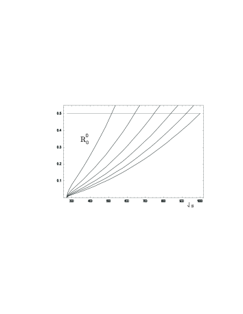
Figure 4: Real part of the $I=0$ $S$-wave amplitude due to the current algebra term plotted for the following increasing values of $N_{c}$ (from left to right), $3$, $5$, $7$, $9$, $11$, $13$. Harada-Sannino-Schechter:04

Next, I show that this result is strongly modified by the presence of the well established $q\bar{q}$ companion of the pion – the $\rho$ meson. The amplitude is obtained by adding to the current algebra contribution the $\rho$ meson contribution given in Eq. (36). In Fig. 5, I show the plot of $R^{0}_{0}$ due to current algebra plus the $\rho$ contribution for increasing values of $N_{c}$.

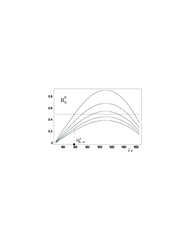
Figure 5: Real part of the $I=0$ $S$-wave amplitude due to the current algebra $+\rho$ terms, plotted for the following increasing values of $N_{c}$ (from up to down), $3$, $4$, $5$, $6$, $7$. The curve with largest violation of the unitarity corresponds to $N_{c}=3$ while the ones within the unitarity bound are for $N_{c}=6,7$. Harada-Sannino-Schechter:04

Here the scaling property of the $\rho$-$\pi$-$\pi$ coupling is taken as $g_{\rho\pi\pi}(N_{c})/g_{\rho\pi\pi}(N_{c}=3)=\sqrt{3/N_{c}}$ with $m_{\rho}$ kept fixed. This figure shows that the unitarity (i.e., $|R_{0}^{0}|\leq 1/2$) is satisfied for $N_{c}\geq 6$ till well beyond the 1 GeV region. However unitarity is still a problem for $3$, $4$ and $5$ colors.

As I showed in Fig. 3, the violation of the unitarity in the real-life QCD is recovered by the existence of the $\sigma$ pole. The $\sigma$ pole structure is such that the real part of its amplitude is positive for $s<M^{2}_{\sigma}$ and negative for $s>M^{2}_{\sigma}$. Identifying the squared sigma mass roughly with $s^{\ast}$, at which $R_{0}^{0}$ without $\sigma$ contribution violates unitarity, will then give a negative contribution where the real part of the amplitude exceeds $+0.5$. In the case when only the current algebra term is included we get

$$M^{2}_{\sigma}\approx s^{\ast}_{ca}=4\pi\,F^{2}_{\pi}\ .$$ (40)

This shows that the squared mass of the $\sigma$ meson needed to restore unitarity for $N_{c}=3,4,5$ increases roughly linearly with $N_{c}$. This estimate gets modified a bit when we include the vector meson (see Fig. 6), yielding $M^{2}_{\sigma}\approx s^{\ast}_{ca+\rho}$, where $s^{\ast}_{ca+\rho}$ is to be obtained from Fig. 5.

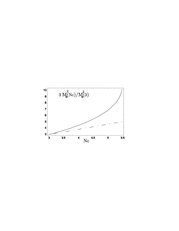
Figure 6: The value $M^{2}(N_{c})$ as a function of $N_{c}$ and normalized to $M^{2}(3)/3$. Harada-Sannino-Schechter:04 The dashed line corresponds to the pure current algebra contribution while the solid line to current algebra $+\rho$ contribution.

This clearly shows that the mass of $\sigma$ becomes larger for larger $N_{c}$, and when $N_{c}\geq 6$, the $\sigma$ is not needed in the energy region below 2 GeV. From this we concluded Harada-Sannino-Schechter:04 that the $\sigma$ meson is unlikely the 2-quark state and likely the 4-quark state. This is similar to the conclusion obtained in Ref. largeNc:pipi .

V Summary

In this write-up, focusing on the structure of the low-lying scalar nonet, I summarized the analyses in two works BHS ; Harada-Sannino-Schechter:04 which I have done recently.

In section II, following Refs. Black-Fariborz-Sannino-Schechter:99 ; Fariborz-Schechter , I first briefly reviewed what the hadronic processes involving the scalar nonet tell about the quark structure of the low-lying scalar mesons. The analysis on the pattern of the hadronic processes implies that the scalar nonet takes dominantly the $qq\bar{q}\bar{q}$ structure (or the diquark–anti-diquark structure). Next, in section III, I summarized the work in Ref. BHS , in which we analyzed the radiative decays involving the scalar nonet based on the $qq\bar{q}\bar{q}$ picture. I also presented a new result BHS:prep on the radiative decays based on the $q\bar{q}$ picture. Our result indicates that it is difficult to distinguish two pictures just from radiative decays. Finally, in section IV, I summarized the work in Ref. Harada-Sannino-Schechter:04 , in which we studied the $\pi$-$\pi$ scattering in large $N_{c}$ QCD. Our analysis shows that the mass of the $\sigma$ meson becomes larger for larger $N_{c}$, and when $N_{c}\geq 6$, the $\pi$-$\pi$ scattering amplitude satisfies the unitarity without the $\sigma$ meson. From this we concluded that the $\sigma$ meson is unlikely the $q\bar{q}$ state and likely the $qq\bar{q}\bar{q}$ state.

References

- (1) See, e.g., the conference proceedings, S. Ishida et al, “Possible existence of the sigma moson and its implication to hadron physics”, KEK Proceedings 2004, Soryushiron Kenkyu 102, No. 5, 2001; D. Amelin and A.M. Zaitsev, “Hadron spectroscopy”, Ninth international conference on hadron spectroscopy, Protvino, Russia (2001); S. Ishida, S. Y. Tsai, T. Komada, K. Takamatsu, T. Tsuru and M. Ishida, “Hadron Spectroscopy, Chiral Symmetry And Relativistic Description Of Bound Systems”, Proceedings, International Symposium, Tokyo, Japan, February 24-26, (2003); A. H. Fariborz, High Energy Physics Workshop “Scalar Mesons: An Interesting Puzzle for QCD”, AIP Conference Proceedings 688 (2003).
- (2) D. Black, A. H. Fariborz, F. Sannino and J. Schechter, Phys. Rev. D 59, 074026 (1999) [arXiv:hep-ph/9808415].
- (3) S. Okubo, Phys. Lett. 5, 165 (1963).
- (4) R. L. Jaffe, Phys. Rev. D 15, 267 (1977).
- (5) A. H. Fariborz and J. Schechter, Phys. Rev. D 60, 034002 (1999) [arXiv:hep-ph/9902238].
- (6) D. Black, M. Harada and J. Schechter, Phys. Rev. Lett. 88, 181603 (2002) [arXiv:hep-ph/0202069]; Prepared for 5th International Conference on Quark Confinement and the Hadron Spectrum, Gargnano, Brescia, Italy, 10-14 Sep 2002; Nucl. Phys. Proc. Suppl. 121, 95 (2003); arXiv:hep-ph/0303223; arXiv:hep-ph/0306065.
- (7) M. Harada, F. Sannino and J. Schechter, Phys. Rev. D 69, 034005 (2004) [arXiv:hep-ph/0309206].
- (8) D. Black, M. Harada and J. Schechter, in preparation.
- (9) D. E. Groom et al. [Particle Data Group Collaboration], Eur. Phys. J. C 15, 1 (2000)
- (10) K. Hagiwara et al. [Particle Data Group Collaboration], Phys. Rev. D 66, 010001 (2002).
- (11) M. Harada, F. Sannino and J. Schechter, Phys. Rev. D 54, 1991 (1996). [hep-ph/9511335].
- (12) D. Black, A. H. Fariborz, F. Sannino and J. Schechter, Phys. Rev. D 58, 054012 (1998) [arXiv:hep-ph/9804273].
- (13) J. Schechter, A. Subbaraman and H. Weigel, Phys. Rev. D 48, 339 (1993) [arXiv:hep-ph/9211239].
- (14) M. Harada and J. Schechter, Phys. Rev. D 54, 3394 (1996) [arXiv:hep-ph/9506473].
- (15) See, e.g., M. Bando, T. Kugo and K. Yamawaki, Phys. Rept. 164, 217 (1988); M. Harada and K. Yamawaki, Phys. Rept. 381, 1 (2003) [arXiv:hep-ph/0302103].
- (16) M. Gell-Mann, D. Sharp and W. G. Wagner, Phys. Rev. Lett. 8, 261 (1962). A general formulation of the interaction in a gauge invariant manner was given in: T. Fujiwara, T. Kugo, H. Terao, S. Uehara and K. Yamawaki, Prog. Theor. Phys. 73, 926 (1985); O. Kaymakcalan, S. Rajeev and J. Schechter, Phys. Rev. D 30, 594 (1984); O. Kaymakcalan and J. Schechter, Phys. Rev. D 31, 1109 (1985); P. Jain, R. Johnson, U. G. Meissner, N. W. Park and J. Schechter, Phys. Rev. D 37, 3252 (1988).
- (17) N. N. Achasov and V. N. Ivanchenko, Nucl. Phys. B 315, 465 (1989); F. E. Close, N. Isgur and S. Kumano, Nucl. Phys. B 389, 513 (1993) [arXiv:hep-ph/9301253]; N. N. Achasov and V. V. Gubin, Phys. Rev. D 56, 4084 (1997) [arXiv:hep-ph/9703367]; Phys. Rev. D 57, 1987 (1998) [arXiv:hep-ph/9706363]; N. N. Achasov, V. V. Gubin and V. I. Shevchenko, Phys. Rev. D 56, 203 (1997) [arXiv:hep-ph/9605245]; J. L. Lucio Martinez and M. Napsuciale, Phys. Lett. B 454, 365 (1999) [arXiv:hep-ph/9903234]; arXiv:hep-ph/0001136; A. Bramon, R. Escribano, J. L. Lucio M., M. Napsuciale and G. Pancheri, Phys. Lett. B 494, 221 (2000) [arXiv:hep-ph/0008188].
- (18) F. Sannino and J. Schechter, Phys. Rev. D 52, 96 (1995) [arXiv:hep-ph/9501417].
- (19) J. R. Pelaez, AIP Conf. Proc. 687, 74 (2003) [arXiv:hep-ph/0306063]. AIP Conf. Proc. 688, 45 (2004) [arXiv:hep-ph/0307018]; Phys. Rev. Lett. 92, 102001 (2004) [arXiv:hep-ph/0309292]; arXiv:hep-ph/0310237: M. Uehara, arXiv:hep-ph/0308241; arXiv:hep-ph/0401037; arXiv:hep-ph/0404221.