1 Introduction

An important unresolved question in the theoretical analysis of charmless non-leptonic $B$ decays is the quantitative understanding of the non-perturbative dynamics responsible for non-factorizable contributions to decay amplitudes.

In the heavy quark limit, $m_{b}\to\infty$ , a factorization theorem [1] states that $B\to PP$ decay amplitudes (where $P$ stands for a light pseudoscalar meson) factorize into perturbatively calculable coefficient functions $T_{\rm I,II}$ and universal hadronic quantities, namely $B\to P$ transition form factors $F^{B\to P}(m_{P}^{2})$ and light-cone wave functions for heavy and light mesons ($\phi_{B}$ and $\phi_{\pi}$). Schematically, one has

$$\langle PP|H_{\rm eff}|B\rangle = F^{B\to P}\cdot T_{\rm I}\otimes\phi_{P}+T_{\rm II}\otimes\phi_{B}\otimes\phi_{P}\otimes\phi_{P}$$ (1)

$${}+\mbox{terms suppressed by $1/m_{b}$}$$

where the symbol $\otimes$ represents convolution with respect to the light-cone momentum fractions of light quarks inside the mesons. Without taking into account radiative corrections, $T_{\rm I}$ depends on kinematic factors only, and $T_{\rm II}$ vanishes. This approximation corresponds to the “naive” factorization assumption. At first order of the strong coupling constant the factorization formula (1) has been shown to hold by the explicit calculation of the $\alpha_{s}$ corrections to naive factorization [1, 2]. In the following we refer to (1) in the heavy-quark limit as “QCD factorization”. Arguments towards an all-order proof have been given in an effective theory framework in [3] (see also [4] for a recent discussion). Here, the relevant momentum modes for $B\to PP$ decays are determined by the momentum scaling of the external particles and their possible interactions. The QCD factorization formula follows from identifying $T_{\rm I,II}$ as coefficient functions of operators in the soft-collinear effective theory (SCET), where the constituents from different hadrons appear to be decoupled. An all-order proof, which considers the subtle effects of endpoint divergences (see Section 2 in [5] for a toy example, and also [6]), has not been worked out to the last detail. It should follow a similar line of reasoning as for the somewhat simpler cases of $B\to\gamma$ and $B\to\pi$ form factors [7, 8, 5, 6].

A major complication for phenomenology arises due to the fact that at least some of the power corrections to (1) appear to be enhanced by large numerical coefficients (these are proportional to the quark condensate in QCD, for this reason these terms are referred to as “chirally enhanced”). In the diagrammatic analysis, non-factorizable contributions are identified from convolution integrals that suffer from endpoint-divergences when one of the parton energies vanishes. The authors of [1] parametrize the chirally enhanced contributions of this type by an arbitrary complex number. The modulus of this number is estimated from regularizing the endpoint divergences with a finite energy cut-off. We emphasize that this is a model-dependent procedure that aims to get a quantitative handle on terms that are beyond the QCD factorization approach. We will refer to this approximation and its phenomenological implications as the “BBNS approach”.

Another well-known framework is to use approximate flavour symmetries (isospin or $SU(3)_{F}$) to relate different decay amplitudes and reduce the number of unknown hadronic parameters [9, 10]. This procedure is often combined with so-called “plausible dynamical assumptions” about the importance of certain flavour topologies that can be identified in the factorization approximation only. In particular, from a recent study in [11] along these lines, it has been concluded that (a) non-factorizable effects in $B\to\pi\pi$ are large, (b) certain $B\to\pi K$ observables point to possible new physics effects in electroweak penguin contributions.

A comprehensive analysis of presently available $B\to PP$ data leads to a somewhat milder conclusion [12]. It is found that, within the statistical uncertainties, the “anomalies” in $B\to\pi K$ decays may still be considered as being consistent with the SM. Furthermore, the non-factorizable effects in $B\to\pi\pi$ can be more or less accounted for by fitting the hadronic input parameters in the BBNS approach to experimental data. Of course, in this procedure, most of the predictive power of the QCD factorization approach is lost. Still, the model-dependent parametrization of non-factorizable effects in the BBNS framework turns out to result in significant constraints when used as the basis for a CKM fit.

The purpose of this article is to carefully examine different (model-dependent) approaches to quantify non-factorizable hadronic effects in charmless non-leptonic $B$ decays. In view of the ultimate goal, namely to extract independent information on CKM parameters from non-leptonic $B$ decays, we think that it is important to make sure that certain assumptions about the size of flavour symmetry breaking, the origin of strong phases etc. are clearly identified in order not to induce an uncontrolled theoretical bias.

Our paper is organized as follows. In the next section we will use the $B\to\pi\pi$ decays as a guideline, and decompose the independent isospin amplitudes into factorizable and non-factorizable parts. The factorizable contributions are estimated within the QCD factorization approach to first order in the strong coupling constant, and using default values for hadronic input parameters. The non-factorizable contributions are considered as unknown parameters, the size of which has to be taken from experimental data on branching fractions and CP asymmetries. We will discuss the origin/interpretation of different sources for non-factorizable effects within the BBNS approach, SCET, and phenomenological studies assuming large long-distance penguin contributions. From this we develop a handful of constrained scenarios that implement different generic features of such approaches. Constraining the parameters for these scenarios using $B\to\pi\pi$ data, one may obtain quite different results on the size of individual isospin amplitudes. In particular, we find that in scenarios with large non-factorizable penguin or annihilation contributions, one may not exclude sizeable corrections to isospin-violating observables which arise from long-distance QED effects, and may be relevant to explain the $B\to\pi K$ puzzles mentioned above. A detailed numerical analysis of $B\to\pi K$ modes is postponed until new experimental data become available.

2 Factorizable and non-factorizable contributions

2.1 Isospin decomposition of decay amplitudes

The CKM elements entering the effective weak hamiltonian for $b$-quark decays in the Standard Model are defined as

$$\lambda_{i}^{(q)} = V_{ib}V_{iq}^{*}\ .$$ (2)

In particular, for $b\to d$ transitions we have

$$\frac{\lambda_{u}^{(d)}}{\lambda_{c}^{(d)}}=-R_{u}\,e^{-i\gamma}\ ,$$ (3)

and for $b\to s$ transitions we have

$$\frac{\lambda_{u}^{(s)}}{\lambda_{c}^{(s)}}=\tan^{2}\theta_{C}\,R_{u}\,e^{-i\gamma}\equiv\epsilon_{KM}\,e^{-i\gamma}$$ (4)

with $\sin\theta_{C}\simeq 0.2266$ being the Cabbibo angle, and $R_{u}=\sqrt{\tilde{\rho}^{2}+\tilde{\eta}^{2}}\simeq 0.405$ and $\gamma\simeq 62^{\circ}$ related to one side and one angle of the CKM-triangle (all numbers from [12], $R_{u}$ is sometimes denoted as $R_{b}$). In the case of $b\to d$ decays, all CKM factors are of the same order, whereas for $b\to s$ decays, $\epsilon_{KM}$ is suppressed by two powers of the Cabbibo angle.

Assuming isospin conservation in hadronic matrix elements the $B\to\pi\pi$ decay amplitudes can be decomposed into

$$\sqrt{2}\,\langle\pi^{-}\pi^{0}|H_{\rm eff}|B^{-}\rangle \simeq \lambda_{u}^{(d)}\left[3A_{u}(2,3/2)\right]+\lambda_{c}^{(d)}\left[3A_{c}(2,3/2)\right]\ ,$$ (5)

$$\langle\pi^{+}\pi^{-}|H_{\rm eff}|\bar{B}^{0}\rangle \simeq \lambda_{u}^{(d)}\left[-A_{u}(0,1/2)+A_{u}(2,3/2)\right]\ ,$$ (7)

$$+\lambda_{c}^{(d)}\left[-A_{c}(0,1/2)+A_{c}(2,3/2)\right]$$

$$\sqrt{2}\,\langle\pi^{0}\pi^{0}|H_{\rm eff}|\bar{B}^{0}\rangle \simeq \lambda_{u}^{(d)}\left[A_{u}(0,1/2)+2A_{u}(2,3/2)\right]$$ (9)

$$+\lambda_{c}^{(d)}\left[A_{c}(0,1/2)+2A_{c}(2,3/2)\right]\ ,$$

where the first argument denotes the total isospin $I$ of the final state, and the second argument denotes the isospin $\Delta I$ of the operators in the weak effective hamiltonian. For the charge-conjugated modes one has to replace $\lambda_{i}^{(d)}$ by $\lambda_{i}^{(d)*}$. Thus, the physical $B\to\pi\pi$ amplitudes fulfill the well-known isospin relation

$$A[B^{-}\to\pi^{-}\pi^{0}]-A[\bar{B}^{0}\to\pi^{0}\pi^{0}]-A[\bar{B}^{0}\to\pi^{+}\pi^{-}]/\sqrt{2} = 0\ .$$ (10)

The latter is violated by small quark mass effects and electromagnetic corrections which we discard in the following.

Notice that only electroweak penguin operators contribute to the amplitude $A_{c}(2,3/2)$. These operators have very small Wilson coefficients compared to those in $A_{u}(2,3/2)$. Actually, neglecting the tiny Wilson coefficients $C_{7}$ and $C_{8}$, one can use Fierz identities to relate the matrix elements of ${\cal O}_{9,10}$ with those of ${\cal O}_{1,2}$ and thus obtains

$$\frac{A_{c}(2,3/2)}{A_{u}(2,3/2)} \simeq \frac{3}{2}\,\frac{C_{9}+C_{10}}{C_{1}+C_{2}}={\cal O}(1\%)\ .$$ (11)

The contribution from $A_{c}(2,3/2)$ can therefore be neglected in $B\to\pi\pi$ decays to a very good approximation. This result is based on the structure of the effective electroweak hamiltonian and on the general isospin analysis only [17, 18].

Using this simplification one sometimes introduces an intuitive parametrization, which refers to the flavour topology (“penguin”, “tree” or “colour-suppressed”) of amplitudes that one would obtain in the factorization approximation,

$$\tilde{P} = \lambda_{c}^{(d)*}\,A_{c}(0,1/2)\ ,$$ (12)

$$\tilde{T}\,e^{i\gamma} = \lambda_{u}^{(d)*}\left(A_{u}(0,1/2)-A_{u}(2,3/2)\right)\ ,$$ (13)

$$\tilde{C}\,e^{i\gamma} = -\lambda_{u}^{(d)*}\left(A_{u}(0,1/2)+2A_{u}(2,3/2)\right)\ .$$ (14)

The ratios between these amplitudes can be parametrized in terms of two moduli and two strong phases as

$$d\,e^{i\theta}\equiv-\frac{\tilde{P}}{\tilde{T}}\,e^{i\gamma} = -\frac{1}{R_{u}}\,\frac{A_{c}(0,1/2)}{A_{u}(2,3/2)-A_{u}(0,1/2)}$$ (15)

as a measure for the “penguin-to-tree ratio”, and

$$x\,e^{i\Delta}\equiv\frac{\tilde{C}}{\tilde{T}} = \frac{A_{u}(0,1/2)+2\,A_{u}(2,3/2)}{A_{u}(2,3/2)-A_{u}(0,1/2)}$$ (16)

as a measure for the ratio of “colour-suppressed” to “colour-allowed” tree amplitudes. Beyond the factorization approximation the notion of flavour topologies might be somewhat misleading, whereas the classification in terms of isospin amplitudes is more general.

The isospin amplitudes $A_{i}(I,\Delta I)$ contain contributions from short-distance dynamics (modes with large virtualities in the heavy quark limit) and long-distance dynamics (modes with virtualities of order $\Lambda_{\rm QCD}^{2}$). The short-distance effects can be treated in perturbative QCD, making use of the heavy-quark expansion. The long-distance effects represent hadronic uncertainties. We therefore decompose every isospin amplitude as

$$A_{i}(I,\Delta I) = A_{i}^{F}(I,\Delta I)+A_{i}^{NF}(I,\Delta I)\ .$$ (17)

In “naive” factorization, the amplitudes $A_{i}^{F}$ can be expressed in terms of electroweak Wilson coefficients and hadronic decay constants and form factors. An example for a naively factorizing diagram is shown in Fig. 1, where we also indicate the momentum scaling of external and internal lines [5]: Here and in the following, “s” stands for soft momenta, “c” and “$\bar{\rm c}$” stand for collinear momenta (virtuality $~{}\Lambda^{2}$) in one or the other direction, “hc” and $\overline{\rm hc}$” for hard-collinear momenta (virtuality $~{}\Lambda m_{b}$) in one or the other direction, and “h” for hard modes.

Figure 1: Example for a naively factorizing contribution to $B\to PP$. The labels indicate the scaling of the momentum modes.

In the heavy-quark limit, we can use QCD factorization (1) to improve the quantitative description of the factorizable part $A_{i}^{F}$. The contributions to the first term in (1) come from vertex corrections and penguin contractions as shown in Fig. 2, and from hard spectator scattering as shown in Fig. 3(a). Non-factorizable effects arise from power corrections in the $\Lambda_{\rm QCD}/m_{b}$ expansion. They include the annihilation topologies (see Fig. 4), and cannot be calculated in a reliable way at present.

(a)           (b)

Figure 2: Examples for (a) vertex and (b) penguin corrections to naive factorization in $B\to PP$. The labels indicate the scaling of the momentum modes.

2.2 Factorizable contributions

In [1] the contributions related to $T_{\rm I}$ and $T_{\rm II}$ in (1) are expressed in terms of parameters $a_{i}=a_{i,\rm I}+a_{i,\rm II}$ ($a_{i,\rm II}$ will be restricted to the heavy-quark limit, whereas in $a_{i,\rm I}$ the terms proportional to $r_{\chi}^{\pi}=m_{\pi}^{2}/m_{q}m_{b}$ are kept). The factorizable amplitudes $A_{i}^{F}$ read

$$A_{u}^{F}(0,1/2) = \frac{A_{\pi\pi}}{6}\left(4a_{1}-2a_{2}+6a_{4}^{u}+3a_{7}-3a_{9}+3a_{10}^{u}+r_{\chi}^{\pi}\,(6a_{6}^{u}+3a_{8}^{u})\right)$$ (18)

$$= \left(0.626^{+0.027}_{-0.022}+i\,0.007^{+0.018}_{-0.010}\right)\,A_{\pi\pi}\$$

$$-\ 0.037\left[\frac{0.28}{F_{0}^{B\to\pi}}\,\frac{350~{}{\rm MeV}}{\lambda_{B}}\left(\frac{\langle\bar{u}^{-1}\rangle_{\pi}}{3.3}\right)^{2}\right]\,A_{\pi\pi}\ ,$$

$$A_{u}^{F}(2,3/2) = -\frac{A_{\pi\pi}}{6}\left(2a_{1}+2a_{2}-3a_{7}+3a_{9}+3a_{10}^{u}+3r_{\chi}^{\pi}\,a_{8}^{u}\right)$$ (20)

$$= -\left(0.350^{+0.007}_{-0.008}-i\,0.021^{+0.003}_{-0.004}\right)\,A_{\pi\pi}\$$

$$-\ 0.023\left[\frac{0.28}{F_{0}^{B\to\pi}}\,\frac{350~{}{\rm MeV}}{\lambda_{B}}\left(\frac{\langle\bar{u}^{-1}\rangle_{\pi}}{3.3}\right)^{2}\right]\,A_{\pi\pi}\ ,$$

$$A_{c}^{F}(0,1/2) = \frac{A_{\pi\pi}}{2}\left(2a_{4}^{c}+a_{7}-a_{9}+a_{10}^{c}+r_{\chi}^{\pi}\,(2a_{6}^{c}+a_{8}^{c})\right)$$ (22)

$$= -\left(0.086^{+0.004}_{-0.004}+i\,0.013^{+0.001}_{-0.000}\right)\,A_{\pi\pi}\$$

$$+\ 0.001\left[\frac{0.28}{F_{0}^{B\to\pi}}\,\frac{350~{}{\rm MeV}}{\lambda_{B}}\left(\frac{\langle\bar{u}^{-1}\rangle_{\pi}}{3.3}\right)^{2}\right]\,A_{\pi\pi}\ ,$$

$$A_{c}^{F}(2,3/2) = -\frac{A_{\pi\pi}}{2}\left(-a_{7}+a_{9}+a_{10}^{c}+r_{\chi}^{\pi}\,a_{8}^{c}\right)\simeq 0.004\,A_{\pi\pi}\ ,$$ (24)

where we introduced

$$A_{\pi\pi}=\frac{iG_{F}}{\sqrt{2}}\,(m_{B}^{2}-m_{\pi}^{2})\,F_{0}^{B\to\pi}(m_{\pi}^{2})\,f_{\pi}\ ,$$

which determines the overall normalization of the factorizable amplitudes, and $F_{0}^{B\to\pi}(q^{2})$ is the scalar $B\to\pi$ transition form factor.

(a)           (b)

Figure 3: Hard-scattering contributions to $B\to PP$. (a) Example for one-gluon exchange included in the BBNS analysis. (b) Example for (power-suppressed) higher-order diagram. The labels indicate the scaling of the momentum modes.

(a)           (b)

Figure 4: Annihilation contributions to $B\to PP$. (a) Example for one-gluon exchange included in the BBNS analysis. (b) Example for higher Fock-state-contribution.

The error in the first term of (24) refers to the variation of the factorization scale $\mu$ between $m_{b}/2$ and $2m_{b}$ in the vertex and penguin graphs. The second term denotes the central value for the hard-scattering contribution which has a large uncertainty related to the first inverse moment $\lambda_{B}^{-1}$ of the light-cone distribution amplitude of the $B$ meson. (There are more sources of parametric uncertainties, in particular the scale-dependence of the hard-scattering term, see the numerical discussion in [1]. Notice that for the hard-scattering terms, we considered the electroweak Wilson coefficients at the scale $\mu=m_{b}$.)

In the following numerical discussion we will refer to the central values of the $A_{i}^{F}$ only. Of course, a significant change in the numerical values of $A_{i}^{F}$ would also influence our conclusions about the size of $A_{i}^{NF}$. In particular, one has to keep in mind that quantities like the “colour-suppressed” amplitude $C$ defined in (14) involve large cancellations in naive factorization, and therefore are particularly sensitive to the precise value of hard-scattering and non-factorizable corrections. The question whether the variation of all possible input parameters in the BBNS approach within “reasonable” ranges could reproduce the experimental data has already been studied in [12]. Here we take the point of view that the default values in [1] give a reliable prediction for the factorizable contributions, whereas the BBNS analysis of non-factorizable terms (including the variation of hadronic input parameters) is considered as one option among different alternatives.

The power-corrections to the hard-scattering parameters $a_{i,\rm II}$, and the annihilation parameters $b_{i}$ are considered as part of the unknown functions $A_{i}^{NF}$, which we parametrize as

$$A_{i}^{NF}(I,\Delta I) := r_{i}(I,\Delta I)\,e^{i\phi_{i}(I,\Delta I)}\,A_{\pi\pi}$$ (25)

with $r_{i}>0$ and an arbitrary phase $\phi_{i}$. (As explained above, one can safely set $A_{c}^{NF}(2,3/2)=0$: Even if we allow for an order-of-magnitude enhancement with respect to its factorizable counterpart in (24), we would only get an ${\cal O}(1\%)$ correction to $A_{u}(2,3/2)$.)

2.3 Non-factorizable effects from $B\to\pi\pi$ data

Our general parametrization of non-factorizable effects introduces seven adjustable parameters $r_{u}(0,1/2)$, $\phi_{u}(0,1/2)$, $r_{u}(2,3/2)$, $\phi_{u}(2,3/2)$, $r_{c}(0,1/2)$, $\phi_{c}(0,1/2)$, and $F_{0}^{B\to\pi}$. On the other hand, if we neglect the tiny contribution from $A_{c}(2,3/2)$, on general grounds, we have only five relevant parameters to describe three complex isospin amplitudes for $B\to\pi\pi$ (one overall phase is not observable). Consequently, our parametrization contains some redundancy, which we will keep for the moment. Later we will consider different constrained scenarios, where the number of parameters is less than 5.

Observable	BaBar	Belle	CLEO	Average
${\cal B}[B^{0}\to\pi^{+}\pi^{-}]$	$4.7\pm 0.6\pm 0.2$	$4.4\pm 0.6\pm 0.3$	$4.5^{+1.4+0.5}_{-1.2-0.4}$	$4.55\pm 0.44$
${\cal B}[B^{+}\to\pi^{+}\pi^{0}]$	$5.5^{+1.0}_{-0.9}\pm 0.6$	$5.0\pm 1.2\pm 0.5$	$4.6^{+1.8+0.6}_{-1.6-0.7}$	$5.18^{+0.77}_{-0.76}$
${\cal B}[B^{0}\to\pi^{0}\pi^{0}]$	$2.1\pm 0.6\pm 0.3$	$1.7\pm 0.6\pm 0.2$	$<4.4$	$1.90\pm 0.47$
$C_{\pi\pi}^{+-}$	$-0.19\pm 0.19\pm 0.05$	$-0.58\pm 0.15\pm 0.07$	–	$-0.46\pm 0.13$
$S_{\pi\pi}^{+-}$	$-0.40\pm 0.22\pm 0.03$	$-1.00\pm 0.21\pm 0.07$	–	$-0.73\pm 0.16$
${\cal A}_{\rm CP}[\pi^{+}\pi^{0}]$	$-0.03^{+0.18}_{-0.17}\pm 0.02$	$-0.14\pm 0.24^{+0.05}_{-0.04}$	–	$-0.07\pm 0.14$

Table 1: Experimental results on $B\to\pi\pi$ observables [12]. All branching ratios are CP-averaged and quoted in units of $10^{-6}$. The sign convention for CP-asymmetries is defined in the text.

Our strategy to infer information on the non-factorizable parameters from experimental data is to produce sets of random parameter values, and calculate the corresponding $\chi^{2}$-value by comparing the theoretical branching ratios and CP asymmetries with the experimental measurements in Table 1 . We follow the sign convention of [12],

$$A_{\rm CP}[\pi^{+}\pi^{0}] = \frac{\Gamma[\bar{B}^{-}\to\pi^{-}\pi^{0}]-\Gamma[\bar{B}^{+}\to\pi^{+}\pi^{0}]}{\Gamma[\bar{B}^{-}\to\pi^{-}\pi^{0}]+\Gamma[\bar{B}^{+}\to\pi^{+}\pi^{0}]}\ ,$$ (26)

and

$$S_{\pi\pi}^{+-}=\frac{2{\rm Im}\lambda_{\pi\pi}}{1+|\lambda_{\pi\pi}|^{2}}\ ,\qquad C_{\pi\pi}^{+-}=\frac{1-|\lambda_{\pi\pi}|^{2}}{1+|\lambda_{\pi\pi}|^{2}}\ ,$$ (27)

$$\lambda_{\pi\pi}=\frac{q}{p}\,\frac{{\cal A}[\bar{B}^{0}\to\pi^{+}\pi^{-}]}{{\cal A}[B^{0}\to\pi^{+}\pi^{-}]}\simeq e^{-2i\beta}\,\frac{{\cal A}[\bar{B}^{0}\to\pi^{+}\pi^{-}]}{{\cal A}[B^{0}\to\pi^{+}\pi^{-}]}$$ (28)

The so-obtained $\chi^{2}$ distributions enable us to investigate the generic size and importance of non-factorizable parameters. To generate the sample, we assume uniform distributions of parameter values in the following ranges

$$0.23\leq F_{0}^{B\to\pi}(m_{\pi}^{2})\leq 0.33\ ,$$

$$0\leq r_{u,c}(I,\Delta I)\leq 1.0\ ,$$

$$0^{\circ}\leq\phi_{u,c}(I,\Delta I)\leq 360^{\circ}\ ,$$ (29)

The bound on the scalar form factor is the main theoretical bias. We used a rather conservative estimate of the theoretical uncertainties, which contains the central value $0.28$ used in [1] as well as a recent update $0.26$ for this quantity in the framework of QCD sum rules [19]. The upper bound on $r_{u,c}(I,\Delta I)$ will turn out to be sufficiently large not to induce an additional bias.

Already for the unconstrained scenario we find some interesting patterns, see Fig. 5, where we have plotted the $\chi^{2}$ value against each of the free parameters for a sample of 500 points with $\chi^{2}<10$:

• The value of the scalar $B\to\pi$ form factor is not constrained by the data

• The distribution of the parameter $r_{u}(0,1/2)$ is rather broad, with a slight preference for $r_{u}(0,1/2)=0.5\pm 0.5$. The corresponding phase take values in the range $120^{\circ}<\phi_{u}(0,1/2)<240^{\circ}$. (Notice that for values of $\phi_{u}(0,1/2)$ around $180^{\circ}$ the non-factorizable contributions reduce the value of the “colour-allowed” tree amplitude, which accomodates the experimental fact that the parameter $x$ in (16) is large.)

• We further find $r_{c}(0,1/2)<0.35$, and $r_{u}(2,3/2)<0.8$. The corresponding phases $\phi_{c}(0,1/2)$ and $\phi_{u}(2,1/2)$ show no pronounced preference.

Of course, there are correlations between the different parameters. For instance, there is no solution with small $\chi^{2}$, where all parameters $r_{i}(I,\Delta I)$ are small (relative to the factorizable terms), in other words the default scenario in the BBNS approach is disfavoured by the data (in accordance with similar conclusions in [11, 12, 20]). For illustration we marked solutions which simultaneously fulfill

$$r_{u}(0,1/2)<0.5\ ,\qquad r_{u}(2,3/2)<0.2\ ,\qquad\mbox{and}\qquad r_{c}(0,1/2)<0.1\ ,$$ (30)

and which, in view of the large parametric uncertainties related to hard-scattering and annihilation contributions (see below) may still be viewed as more or less compatible with the BBNS approach (in the spirit of [12]). This still yields values of $\chi^{2}\simeq 3$.

$F_{0}^{B\to\pi}$
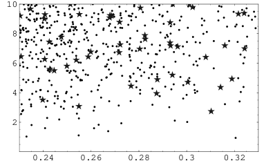
$r_{u}(0,1/2)$	$\phi_{u}(0,1/2)$
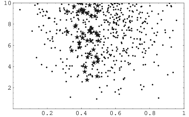
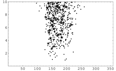
$r_{c}(0,1/2)$	$\phi_{c}(0,1/2)$
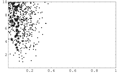
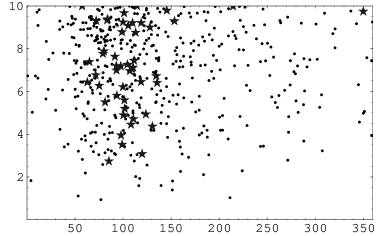
$r_{u}(2,3/2)$	$\phi_{u}(2,3/2)$

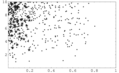
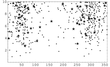
Figure 5: Comparison of $\chi^{2}$ values for a random sample of non-factorizable parameters: Dots for unconstrained scenario, stars for combinations that fulfill (30).

2.4 Non-factorizable effects from “BBNS”

In the BBNS approach non-factorizable effects arise through chirally enhanced power-corrections which are identified from endpoint-divergent convolution integrals, appearing in the diagrammatic approach.

2.4.1 Hard-scattering contributions

One source of non-factorizable power-corrections are so-called hard spectator-scattering diagrams, where a gluon connects the spectator quark to the short-distance decay process. Fig. 3(a) (together with an analogous diagram where the gluon is attached to the other collinear quark) has been considered in [1]. On the other hand, Fig. 3(b) represents an example of a higher-order diagram (which is not included in the BBNS approach), which involves a multi-particle Fock state in the $B$ meson and which is power-suppressed (see below).

Apart from a factorizable part that determines the heavy quark limit, explicit calculation shows that the diagram in Fig. 3(a) gives rise to chirally-enhanced power-suppressed endpoint divergences. At the considered order in the diagrammatic expansion, these endpoint divergences enter through the quantity

$$X_{H}^{\pi} \equiv \int_{0}^{1-\Lambda_{h}/m_{B}}\,\frac{u}{1-u}\,\phi_{p}^{\pi}(u)\ ,$$ (31)

where $\phi_{p}^{\pi}(u)\simeq 1$ is a twist-3 light-cone distribution amplitude of the pion. We regularized the integral by means of an ad-hoc cut-off, because the integral does not converge for $u\to 1$. Since the twist-3 distribution amplitudes are normalized to a term proportional to the quark condensate (i.e. the ratio of Goldstone boson and quark masses, $m_{M}^{2}/m_{q}$), their contributions are numerically large (“chirally enhanced”). To study the phenomenological impact of these terms, the authors of [1] propose to parametrize the quantity on the left-hand side in terms of

$$X_{H}^{\pi} = (1+\rho_{H}\,e^{i\varphi_{H}})\,\ln\frac{m_{B}}{\Lambda_{H}}\ ,\qquad\rho_{H}\sim{\cal O}(1)$$ (32)

with $\varphi_{H}$ being an arbitrary phase, whereas $\Lambda_{H}\approx 0.5$ GeV.

Inserting the default values for the hadronic parameters in the BBNS analysis, we obtain

$$A_{u}^{\rm NF}[0,1/2]|_{\rm hs} \simeq -0.030\,A_{\pi\pi}\,(1+\rho_{H}\,e^{i\varphi_{H}})\left[\frac{0.28}{F_{0}^{B\to\pi}}\,\frac{350~{}{\rm MeV}}{\lambda_{B}}\,\frac{\langle\bar{u}^{-1}\rangle_{\pi}}{3.3}\right]\ ,$$ (33)

$$A_{u}^{\rm NF}[2,3/2]|_{\rm hs} \simeq -0.018\,A_{\pi\pi}\,(1+\rho_{H}\,e^{i\varphi_{H}})\left[\frac{0.28}{F_{0}^{B\to\pi}}\,\frac{350~{}{\rm MeV}}{\lambda_{B}}\,\frac{\langle\bar{u}^{-1}\rangle_{\pi}}{3.3}\right]\ ,$$ (34)

$$A_{c}^{\rm NF}[0,1/2]|_{\rm hs} \simeq 0.001\,A_{\pi\pi}\,(1+\rho_{H}\,e^{i\varphi_{H}})\left[\frac{0.28}{F_{0}^{B\to\pi}}\,\frac{350~{}{\rm MeV}}{\lambda_{B}}\,\frac{\langle\bar{u}^{-1}\rangle_{\pi}}{3.3}\right]\ ,$$ (35)

$$A_{c}^{\rm NF}[2,3/2]|_{\rm hs} \simeq 0\ .$$ (36)

Comparing with the general parametrization (25), we deduce that in the BBNS approach $r_{u}(I,\Delta I)$ are expected to receive contributions of the order 5% (up to 10% for the “large $a_{2}$ scenario”) from hard spectator-scattering, whereas the corresponding effect for $r_{c}(I,\Delta I)$ seems to be negligible.

In any case the above procedure is understood to only give a rough idea about the typical size of non-factorizable contributions for individual decay amplitudes. The origin and size of strong re-scattering phases remains unclear. In particular, treating $\rho_{H}$ and $\varphi_{H}$ as universal parameters, one induces model-dependent correlations between non-factorizable effects in different isospin amplitudes. Substantially different strong interaction phases for, say, $I=0$ and $I=2$ final states can arise from more complicated diagrams with additional quark lines (i.e. higher Fock states). In the diagrammatic approach along the lines of BBNS, these effects can only show up at higher orders in the diagrammatic expansion. Notice that in the case of non-factorizable endpoint configurations, “higher-order” diagrams are not necessarily suppressed by powers of the strong coupling constant. The universality of strong phases arising from hard-spectator scattering is therefore not a generic feature of QCD factorization, but represents an additional phenomenological assumption in the BBNS approach. The analysis [12] uses universal BBNS parameters for all isospin amplitudes. Different phases in different isospin amplitudes can still be generated by combining the non-factorizing pieces from hard scattering ($X_{H}$) and from annihilation ($X_{A}$ see below) which are treated as independent complex parameters. Nevertheless, a model-dependent correlation between non-factorizable contributions to different $B\to\pi\pi$ and $B\to\pi K$ amplitudes remains. The implications of that analysis should therefore be interpreted with some care.

2.4.2 Scenario 1: Dominance of hard spectator scattering

If we assume that non-factorizable effects from power-suppressed contributions to hard spectator scattering (or alternatively, significant changes of hadronic input parameters in the factorizable pieces) are the main source for $A^{\rm NF}(I,\Delta I)$, we may define a phenomenological approximation, where we put $r_{c}(0,1/2)=0$. In addition, we might either fix the form factor value, $F_{0}=0.26$ (Scenario 1a), or assume that the phases $\varphi_{H}$ are universal such that $\phi_{u}(0,1/2)=\phi_{u}(2,1/2)$ (Scenario 1b).

Repeating the analysis of the $B\to\pi\pi$ data with these additional constraints, we obtain the situation illustrated in Figs. 6 and 7. Scenario 1a still gives a more or less reasonable description with $\chi^{2}\geq 4$ for six experimental observables and four adjustable parameters. The situation in Scenario 1b is similar, but somewhat worse. In both cases we need rather large non-factorizable amplitudes with either $r_{u}(0,1/2)>0.5$ or $r_{u}(2,3/2)>0.3$. $\phi_{u}(0,1/2)$ is rather constrained in both cases.

$r_{u}(0,1/2)$	$\phi_{u}(0,1/2)$
$r_{u}(2,3/2)$	$\phi_{u}(2,3/2)$

Figure 6: Comparison of $\chi^{2}$ values for a random sample of non-factorizable parameter combinations, using $r_{c}(0,1/2)=0$ and $F_{0}^{B\to\pi}=0.26$ (Scenario 1a).

$r_{u}(0,1/2)$	$\phi_{u}(0,1/2)$
$r_{u}(2,3/2)$	$F_{0}^{B\to\pi}$

Figure 7: Comparison of $\chi^{2}$ values for a random sample of non-factorizable parameter combinations, using $r_{c}(0,1/2)=0$ and $\phi_{u}(2,3/2)=\phi_{u}(0,1/2)$ (Scenario 1b).

2.4.3 Annihilation topologies

Another source of non-factorizable, power-suppressed contributions to $B\to PP$ are annihilation topologies, see Fig. 4. They receive the same chiral enhancement as the non-factorizable hard-scattering pieces.

In the BBNS approach, the flavour-changing sub-process for annihilation topologies is $bq\to q\bar{q}$, and consequently, it can only contribute to $I=0$ (for $B\to\pi\pi$) or $I=1/2$ (for $B\to\pi K$) decay amplitudes (again this statement is only true as long as we do not consider higher Fock states). The order of magnitude for annihilation effects is estimated in a similar way as for the hard-scattering terms in the previous section, introducing the quantity

$$X_{A}^{\pi} = (1+\rho_{A}\,e^{i\varphi_{A}})\,\ln\frac{m_{B}}{\Lambda_{H}}\ ,\qquad\rho_{A}\sim{\cal O}(1)\ .$$ (37)

The corresponding contributions to the non-factorizable $B\to\pi\pi$ amplitudes read

$$A_{u}(0,1/2)|_{\rm ann} \simeq 0.01\,(1+1.0\rho_{A}e^{i\varphi_{A}}-0.7\rho_{A}^{2}e^{2i\varphi_{A}})\,A_{\pi\pi}\ ,$$ (38)

$$A_{c}(0,1/2)|_{\rm ann} \simeq -0.01\,(1+2.0\rho_{A}e^{i\varphi_{A}}+0.9\rho_{A}^{2}e^{2i\varphi_{A}})\,A_{\pi\pi}\ .$$ (39)

Comparing with the general parametrization (25), we deduce that in the BBNS approach $r_{u,c}[0,1/2]$ may receive contributions of the order of several percent from annihilation. Notice that the annihilation topologies in BBNS lead to $1/m_{b}^{2}$ corrections that are doubly chirally enhanced (giving rise to the $\rho_{A}^{2}$ terms above).

2.4.4 Scenario 2: Dominance of annihilation topologies

In another approximation, we assume that the non-factorizable part of the $\Delta I=3/2$ amplitude is sub-dominant and can be neglected, $r_{u}(2,3/2)=0$. In addition we again fix the form factor, $F_{0}^{B\to\pi}=0.26$.

From the theoretical point of view, the situation corresponds to the case where the annihilation graphs in the BBNS approximation are assumed to be the dominant source of non-factorizable effect. Alternatively, it can also be viewed as representing the case where higher-order contributions from penguin corrections (“charm” and “GIM” penguins [21, 22]; for a recent phenomenological fit along these lines, see [23]) are the main source of non-factorizing effects (again, such effects do not contribute to the amplitudes with $\Delta I=3/2$).

From the plots in Fig. 8 we observe that a very good description of the data is possible in such a scenario. Again, rather large non-factorizable effects (i.e. of the same order as the factorizable ones) are needed in $A_{u}(0,1/2)$ and/or $A_{c}(0,1/2)$. The data also show a clear prefererence for $A_{c}^{\rm NF}(0,1/2)<A_{u}^{\rm NF}(0,1/2)$ in this scenario.

$r_{u}(0,1/2)$	$\phi_{u}(0,1/2)$
$r_{c}(0,1/2)$	$\phi_{c}(0,1/2)$

Figure 8: Comparison of $\chi^{2}$ values for a random sample of non-factorizable parameter combinations, using $A_{u}^{\rm NF}(2,3/2)=0$ and $F_{0}^{B\to\pi}=0.26$ (Scenario 2 – dominance of annihilation/penguins).

2.5 Non-factorizable contributions in SCET

Soft-collinear effective theory has been developped as a systematic tool to study the factorization of different short- and long-distance modes contributing to inclusive and exclusive $B$ decays [24, 25, 26]. In case of exclusive decays, two kinds of short-distance modes are successively integrated out: hard modes (with virtualities of order $m_{b}^{2}$) and hard-collinear modes (with energies of order $m_{b}$ and virtualities of order $m_{b}\Lambda_{\rm QCD}$) [27, 28, 5]. The first matching step leads from QCD to the so-called SCET_I. The second matching step leads from SCET_I to SCET_II. The effective theory SCET_II only contains long-distance modes with virtualities of the order of the QCD scale. In the $B$ meson rest frame these are denoted as “soft” (all momentum components of order $\Lambda_{\rm QCD}$), and “collinear” (one momentum component scales as $m_{b}$). Fields and operators in the effective theory have a definite power-counting in terms of the expansion parameter $\lambda^{2}=\Lambda_{\rm QCD}/m_{b}$. In this paragraph we will discuss some generic examples for effective-theory operators that may give rise to factorizable and/or non-factorizable effects in $B\to\pi\pi$.

Let us follow the strategy of [5] (which has been used in the context of a factorization proof for the $B\to\pi\ell\nu$ decay) and identify the possible field content of effective operators in SCET_I that are relevant for $B\to\pi\pi$. (We will consider light-cone gauge for the collinear modes, and will drop soft Wilson lines for simplicity. We also do not explicitely note Dirac or Lorentz indices.). The two hard-collinear directions defined by the final-state hadron are denoted as “hc” and “$\overline{\rm hc}$”, respectively. It is understood that for all operators that we will list below, one has a corresponding term with ${\rm hc}\leftrightarrow\overline{\rm hc}$ interchanged. It should also be clear that the different possible flavour structures of the operators in SCET are obtained from matching the corresponding operators in the weak effective hamiltonian by integrating out hard QCD modes (we will comment on flavor-dependent QED effects below).

In the second matching step, one has to generate the minimal field content

$$[\bar{q}_{s}\ldots h_{v}]\,[\bar{\xi}_{c}\ldots\xi_{c}]\,[\bar{\xi}_{\bar{c}}\ldots\xi_{\bar{c}}]$$

that is necessary to build up the initial and final state quantum numbers (the dots stand for additional $q\bar{q}$ pairs or gluon fields of the same kind; we do not consider decays into flavor-singlet mesons here). The generation of soft and collinear fields from hard-collinear ones costs a certain power of the small expansion parameter $\lambda$, which can be read off the corresponding interaction terms in the SCET_I Lagrangian. Examples are [5]

$$\xi_{\rm hc} \stackrel{{\scriptstyle\lambda}}{{\rightarrow}} \xi_{c}\ ,$$ (40)

$$\xi_{\rm hc} \stackrel{{\scriptstyle\lambda^{2}}}{{\rightarrow}} \xi_{c}\,A^{\perp}_{\rm hc}\ ,$$ (41)

$$A^{\perp}_{\rm hc} \stackrel{{\scriptstyle\lambda}}{{\rightarrow}} \bar{q}_{s}\xi_{\rm hc}\ ,$$ (42)

$$A^{\perp}_{\rm hc} \stackrel{{\scriptstyle\lambda^{2}}}{{\rightarrow}} \bar{q}_{s}\xi_{c}\ .$$ (43)

2.5.1 3-body operators

The minimal possible field content for a SCET_I operator, that contributes to $B\to\pi\pi$, is

$$[\bar{\xi}_{\rm hc}\,A_{\overline{\rm hc}}^{\perp}\,h_{v}]\sim\lambda^{5}\ ,$$ (44)

where on the right-hand side we indicated the power-counting for this operator, following from the SCET_I Lagrangian. Performing the explicit matching calculation, one finds that at tree-level the first non-trivial operator is just a copy of the chromomagnetic term $O_{8}^{g}$ in the weak hamiltonian, restricted to the particular kinematical situation,

$$-C_{8}^{\rm eff}\,\frac{g_{s}m_{b}}{8\pi^{2}}\,\bar{\xi}_{\rm hc}\,\sigma_{\mu\nu}(1+\gamma_{5})\,G^{\mu\nu}_{\rm\overline{hc}}\,h_{v}+({\rm hc}\to\overline{\rm hc})\ .$$ (45)

Here $C_{8}^{\rm eff}$ contains the short-distance contribution from loop contractions with 4-quark penguin operators.

Starting from the operator in (45), in order to generate the necessary final-state partons, we need at least two collinear quark fields $\xi_{c}$ and $\bar{\xi}_{c}$ which have to be generated from the hard-collinear field $\bar{\xi}_{\rm hc}$, and two collinear quark fields $\xi_{\bar{c}}$ and $\bar{\xi}_{\bar{c}}$ which should descend from $A^{\perp}_{\overline{\rm hc}}$. The first case costs at least a factor $\lambda^{4}$, for instance through the chain

$$\bar{\xi}_{\rm hc}\stackrel{{\scriptstyle\lambda^{2}}}{{\rightarrow}}\bar{\xi}_{c}A_{\rm hc}^{\perp}\stackrel{{\scriptstyle\lambda^{2}}}{{\rightarrow}}\bar{\xi}_{c}[\bar{q}_{s}\xi_{c}]\ .$$ (46)

In the second case, we cannot directly produce two collinear quark fields from the hard-collinear gluon field, because they would be in a flavor-singlet configuration (the case of flavor-singlet mesons has been discussed in the context of QCD factorization in [29]). Therefore we need at least two additional quark fields that do not end up in the corresponding pion (and therefore have to come from the initial $B$ meson which provides soft modes). A possible branching

$$A_{\rm\bar{h}c}^{\perp}\stackrel{{\scriptstyle\lambda}}{{\rightarrow}}\bar{q}_{s}\xi_{\overline{\rm hc}}\stackrel{{\scriptstyle\lambda^{4}}}{{\rightarrow}}[\bar{q}_{s}\xi_{\bar{c}}][\bar{\xi}_{\bar{c}}q_{s}]$$ (47)

costs a factor $\lambda^{5}$ such that the power-counting for currents in SCET_II that descend from three-body operators in SCET_I is $\lambda^{14}$. Together with the power-counting for the hadronic states the contribution to the $B\to\pi\pi$ amplitude is $\lambda^{7}$, which has to be compared with the result in naive factorization $\sim f_{\pi}F_{0}^{B\to\pi}\sim\lambda^{5}$. Therefore, contributions from three-body operators are $1/m_{b}$ suppressed (and therefore do not contribute to the factorization theorem in the heavy-quark limit). To obtain a non-vanishing contribution of a 3-body SCET_I operator to a $B\to\pi\pi$ matrix element in the diagrammatic expansion of the BBNS approach, we thus need at least three gluons, see Fig. 3(b). Such diagrams are not considered in the analysis of power-corrections in [1], which has been restricted to one-gluon exchange diagrams. Up to now, we do not know whether this operator gives factorizable contributions in the first non-vanishing order in SCET_II (i.e. $1/m_{b}$ with respect to the leading contributions from naive factorization). In any case, from the structure of the factorization proof for $B\to\pi\ell\nu$ decays in [5] and similar arguments in [33], we expect that, in general, factorization of soft and collinear modes in SCET_II does not hold for power-corrections obtained in the matching of SCET_I to SCET_II. Therefore, at least on the level of $1/m_{b}^{2}$ power-corrections, the operator in (45) provides a new source of non-factorizable corrections. Similarly as for the annihilation diagrams considered in BBNS, see (37), contributions from such power-suppressed 8-quark operators in SCET_II could be doubly chirally enhanced. In this case, numerically they may be as important as the non-factorizable terms included in the BBNS analysis.

2.5.2 4-body operators

The leading-power contributions to the function $T_{\rm I}$ in (1) involve four-quark operators in SCET_I of the type

$$[\bar{\xi}_{\rm\overline{\rm hc}}\xi_{\rm hc}][\bar{\xi}_{\rm hc}h_{v}]\sim\lambda^{6}\ .$$ (48)

The conversion of the hard-collinear quark pair to a collinear one costs twice a power of $\lambda$, and the conversion of $\bar{\xi}_{\rm\overline{\rm hc}}$ via (46) costs a factor of $\lambda^{4}$. Therefore, these four-quark operators match onto 6-quark operators in SCET_II which scale as $\lambda^{12}$ and, according to the discussion in the previous paragraph, are leading power.

Another 4-quark operator that is allowed in SCET_I by momentum conservation is of the form

$$[\bar{q}_{s}h_{v}][\bar{\xi}_{\rm\overline{\rm hc}}\xi_{\rm hc}]\sim\lambda^{8}\ .$$ (49)

The conversion of hard-collinear quark fields into at least two collinear fields via (46) costs each a factor of $\lambda^{4}$. Therefore, these operators match onto 8-quark operators in SCET_II which scale at least as $\lambda^{16}$ and are thus $1/m_{b}^{2}$ suppressed. This corresponds to an annihilation topology which involves a higher Fock state $(b\bar{q})(q^{\prime}\bar{q}^{\prime})$ in the $B$ meson. Notice that, again, the suppression by $1/m_{b}^{2}$ can be numerically compensated by two chiral enhancement factors coming from the wave functions of the two final-state mesons.

We may also consider 4-body operators that involve additional gluons, like

$$[A^{\perp}_{\rm\overline{\rm hc}}][\bar{\xi}_{\rm hc}A^{\perp}_{\rm hc}h_{v}]\sim\lambda^{6}\quad\stackrel{{\scriptstyle{\rm SCET}_{\rm II}}}{{\rightarrow}}\quad\int\ldots[\bar{q}_{s}\xi_{\bar{c}}][\bar{\xi}_{\bar{c}}q_{s}][\bar{q}_{s}\xi_{c}][\bar{\xi}_{c}h_{v}]\sim\lambda^{14}\ ,$$ (50)

or

$$[A^{\perp}_{s}A^{\perp}_{\rm hc}][\bar{\xi}_{\overline{\rm hc}}h_{v}]\sim\lambda^{7}\quad\stackrel{{\scriptstyle{\rm SCET}_{\rm II}}}{{\rightarrow}}\quad\int\ldots A^{\perp}_{s}[\bar{q}_{s}\xi_{\bar{c}}][\bar{\xi}_{\bar{c}}q_{s}][\bar{q}_{s}\xi_{c}][\bar{\xi}_{c}h_{v}]\sim\lambda^{16}\ ,$$ (51)

where again we have to use (47) to obtain flavour non-singlet collinear quark configurations from a single hard-collinear gluon field.

2.5.3 Remark on the treatment of charm quarks

One may also worry about 4-quark operators involving charm quarks. In the BBNS approach, the charm quarks are treated as hard modes (i.e. $m_{c}={\cal O}(m_{b})$), and therefore they are integrated out in the first matching step and do not appear as degrees of freedom in SCET_I. Alternatively, one may take the point of view that $m_{c}^{2}\sim\Lambda m_{b}$, i.e. $m_{c}\ll m_{b}$ in the heavy quark limit. Still, since charm quarks do not appear as external partonic degrees of freedom in charmless non-leptonic $B$ decays, they cannot induce endpoint singularities, and can, in any case, be treated perturbatively. The effect of the alternative power-counting scheme merely amounts to expanding the hard coefficient functions in terms of $m_{c}/m_{b}$, which corresponds to integrating out the charm quarks in the second matching step SCET_I $\to$ SCET_II. Via the renormalization group running within SCET_I one would also resum logarithms $\ln m_{c}/m_{b}$. Numerically, the effect onto factorizable amplitudes should be marginal. In the non-factorizable contributions, on the other hand, the crucial effects come from the endpoint divergences and chiral enhancement related to light quarks, and not from charm quarks, if $m_{c}\gg\Lambda_{\rm QCD}$.

In [4] it has been argued that one should also consider the possibility of non-relativistic charm and gluon modes in SCET_I. This would correspond to operators of the type

$$[\bar{\xi}_{\overline{\rm hc}}h_{v}][\bar{c}c]_{\rm NR}\ ,$$

where the invariant mass of the $c\bar{c}$ pair happens to be close to $4m_{c}^{2}$ which corresponds to a light-cone momentum fraction for the quark field $\bar{\xi}_{\overline{\rm hc}}$ of the order $u=1-4m_{c}^{2}/m_{b}^{2}\simeq 0.6$. However, since charm modes do not appear as external degrees of freedom, hadronic matrix elements of the above operator in SCET${}_{\rm I}\times$ NRQCD would vanish. One may ask the question, where the effect of charm resonances (i.e. non-relativistic $c\bar{c}$ bound states, $J/\psi,\psi^{\prime},\ldots$) would show up in the effective theory framework. As explained above, as charm quarks do not appear as external states, they can be formally integrated out, resulting in a quark determinant with charm quarks in the background of soft and collinear gluon fields. The treatment of charm quarks is thus fully inclusive, and the appearance of charm resonances resembles the well-known cases of $e^{+}e^{-}\to\mbox{hadrons}$ or $B\to X_{s}\ell^{+}\ell^{-}$: When integrating the invariant-mass spectrum over a large enough region, the effect of charm resonances provides power-corrections to the inclusive rate.

In our case, the pion distribution amplitude serves as the “detector” with a “sensitivity” $\phi_{\pi}(u=1-q^{2}/m_{b}^{2})$. Integrating over all momentum fractions $u$, the effect of charm resonances translates into power-corrections, which should be attributed to the matching coefficients of sub-leading operators in SCET_I. One can even perform a numerical estimate of such charm-resonance effects by using the same phenomenological treatment as for $b\to s\ell^{+}\ell^{-}$ [30, 31]. We find that the standard pion distribution amplitude is sufficiently broad to wash out the effect of exclusive charm resonances. Therefore it is not clear to us in what sense the inclusion of non-relativistic modes in SCET_I should lead to an enhancement of charm penguin contributions in non-leptonic $B$ decays, as has been argued in [4]. Also in a recent analysis within QCD sum rules [32], an unnatural enhancement of charm-penguin contributions to non-leptonic $B$ decays is not observed, and the perturbative treatment of charm quarks seems to be justified.

2.5.4 5-body operators

Two examples of 4-quark operators with an additional hard-collinear gluon are

$$[\bar{\xi}_{\rm hc}\xi_{\overline{\rm hc}}][\bar{\xi}_{\overline{\rm hc}}A_{\rm hc}^{\perp}h_{v}] \sim \lambda^{7}\ ,$$ (52)

$$[\bar{\xi}_{\rm hc}A_{\rm hc}^{\perp}\xi_{\rm hc}][\bar{\xi}_{\overline{\rm hc}}h_{v}] \sim \lambda^{7}\ .$$ (53)

With similar arguments as above, the first term matches onto a leading-power 6-quark operator in SCET_II, which corresponds to the factorizable hard-spectator diagrams in the QCD factorization approach. The second term gives a $1/m_{b}$ power-suppressed contribution, which serves as one of the candidates to compensate the endpoint divergences parametrized by $X_{H}$. There are a number of further 5-body structures, which we are not going to discuss in detail here.

2.5.5 6-body operators

The simplest 6-quark operator in SCET_I has the form

$$[\bar{\xi}_{\rm hc}\xi_{\overline{\rm hc}}][\bar{\xi}_{\overline{\rm hc}}\xi_{\rm hc}][\bar{q}_{s}h_{v}]\sim\lambda^{10}$$ (54)

The leading-power matching onto SCET_II gives a 6-quark operator of the order $\lambda^{14}$ which corresponds to the $1/m_{b}$-suppressed annihilation graphs in the BBNS approach.

Another possibility is a 4-quark operator with two additional transverse gluons, e.g.

$$[\bar{\xi}_{\rm hc}\xi_{\overline{\rm hc}}][\bar{q}_{s}h_{v}]A_{\rm hc}^{\perp}A_{\overline{\rm hc}}^{\perp}\sim\lambda^{10}$$ (55)

which amounts to annihilation with additional radiation of hard-collinear gluons. After matching onto SCET_II, the minimal quark content refers to an 8-quark operator which scales as $\lambda^{16}$, and is therefore $1/m_{b}^{2}$ suppressed with respect to the leading-power contributions, and should be related to the terms of order $X_{A}^{2}$ in (37).

2.5.6 Summary: Factorizable and non-factorizable SCET operators

We summarize the examples for SCET_I and SCET_II operators in Table 2. The identification of the power-corrections as non-factorizable is tentative (without a more detailed analysis, which is beyond the scope of this work, we cannot exclude that some of the operators identified as non-factorizable at a certain sub-leading power in $1/m_{b}$ are actually free of endpoint divergences in SCET_II). The factorization of the two structures contributing at leading power (as indicated by $\surd$), can be understood by applying the same rules as in the $B\to\pi\ell\nu$ case [5] (this point has also been realized in [4]).

Notice that another set of possible operators is obtained by changing one gluon field into a photon field. The contributions of such operators are suppressed by the ratio of electromagnetic and strong coupling constants, $\alpha_{\rm em}/\alpha_{s}$. They may be important in isospin-breaking observables for $B\to\pi K$ decays, if they enter with large Wilson coefficients and large CKM elements, and if the $1/m_{b}$ suppression is compensated by large numerical factors.

SCETI	power	$A^{\rm F}$	$A^{\rm NF}$	SCETII	BBNS
$[\bar{\xi}_{\rm hc}\,A^{\perp}_{\overline{\rm hc}}\,h_{v}]$	$\lambda^{5}$	–	$1/m_{b}$	$[\bar{q}_{s}\bar{q}_{s}..q_{s}h_{v}][\bar{\xi}_{\bar{c}}..\xi_{\bar{c}}][\bar{\xi}_{c}..\xi_{c}]$
$[\bar{\xi}_{\rm\overline{\rm hc}}\xi_{\rm hc}][\bar{\xi}_{\rm hc}h_{v}]$	$\lambda^{6}$	$\surd$	$1/m_{b}$	$[\bar{q}_{s}..h_{v}][\bar{\xi}_{\bar{c}}..\xi_{\bar{c}}][\bar{\xi}_{c}..\xi_{c}]$	in $T_{\rm I}$
$[A^{\perp}_{\rm\overline{\rm hc}}][\bar{\xi}_{\rm hc}A^{\perp}_{\rm hc}h_{v}]$	$\lambda^{6}$	–	$1/m_{b}$	$[\bar{q}_{s}\bar{q}_{s}..q_{s}h_{v}][\bar{\xi}_{\bar{c}}..\xi_{\bar{c}}][\bar{\xi}_{c}..\xi_{c}]$
$[\bar{\xi}_{\rm hc}\xi_{\overline{\rm hc}}][\bar{\xi}_{\overline{\rm hc}}A_{\rm hc}^{\perp}h_{v}]$	$\lambda^{7}$	$\surd$	$1/m_{b}$	$[\bar{q}_{s}..h_{v}][\bar{\xi}_{\bar{c}}..\xi_{\bar{c}}][\bar{\xi}_{c}..\xi_{c}]$	in $T_{\rm II}$, $X_{H}$
$[\bar{\xi}_{\rm hc}A_{\rm hc}^{\perp}\xi_{\rm hc}][\bar{\xi}_{\overline{\rm hc}}h_{v}]$	$\lambda^{7}$	–	$1/m_{b}$	$[\bar{q}_{s}..h_{v}][\bar{\xi}_{\bar{c}}..\xi_{\bar{c}}][\bar{\xi}_{c}..A_{c}^{\perp}\xi_{c}]$
$[A^{\perp}_{s}A^{\perp}_{\rm hc}][\bar{\xi}_{\overline{\rm hc}}h_{v}]$	$\lambda^{7}$	–	$1/m_{b}^{2}$	$[\bar{q}_{s}\bar{q}_{s}..A_{s}^{\perp}q_{s}h_{v}][\bar{\xi}_{\bar{c}}..\xi_{\bar{c}}][\bar{\xi}_{c}..\xi_{c}]$
$[\bar{q}_{s}h_{v}][\bar{\xi}_{\rm\overline{\rm hc}}\xi_{\rm hc}]$	$\lambda^{8}$	–	$1/m_{b}^{2}$	$[\bar{q}_{s}\bar{q}_{s}..q_{s}h_{v}][\bar{\xi}_{\bar{c}}..\xi_{\bar{c}}][\bar{\xi}_{c}..\xi_{c}]$
$[\bar{\xi}_{\rm hc}\xi_{\overline{\rm hc}}][\bar{\xi}_{\overline{\rm hc}}\xi_{\rm hc}][\bar{q}_{s}h_{v}]$	$\lambda^{10}$	–	$1/m_{b}$	$[\bar{q}_{s}..h_{v}][\bar{\xi}_{\bar{c}}..\xi_{\bar{c}}][\bar{\xi}_{c}..\xi_{c}]$	in $X_{A}$
$[\bar{\xi}_{\rm hc}\xi_{\overline{\rm hc}}][\bar{q}_{s}h_{v}]A_{\rm hc}^{\perp}A_{\overline{\rm hc}}^{\perp}$	$\lambda^{10}$	–	$1/m_{b}^{2}$	$[\bar{q}_{s}\bar{q}_{s}..q_{s}h_{v}][\bar{\xi}_{\bar{c}}..\xi_{\bar{c}}][\bar{\xi}_{c}..\xi_{c}]$
…	…	…	…	…	…

Table 2: An incomplete list of the field content of SCET_I operators, contributing to non-leptonic $B$ decays into light hadrons. See text for details.

2.6 Non-factorizable effects from long-distance penguins

(a)           (b)         

Figure 9: Examples for (a) short- and (b) long-distance penguin contributions to a 4-body Greens function in SCET_I via hard, hard-collinear or soft quark loop.

It is often argued that a main source of non-factorizable effects in $B\to PP$ decays should be attributed to long-distance penguin topologies [21, 22], where two quarks of one of the four-quark operators ${\cal O}_{1-6}$ in the electroweak hamiltonian are contracted to a loop which radiates one or more gluons. As explained above, in the effective theory approach, long-distance modes in SCET_I are hard-collinear and soft quark and gluon fields, i.e. the effect of $b$ (and usually also $c$) quarks is already absorbed into matching coefficients, see Fig. 9(a). Examples for long-distance penguin diagrams in SCET_I are shown in Fig. 9(b). They reflect contributions to one of the 4-body operators (49) discussed above, which gives power-suppressed contributions to the decay amplitudes. Remember that above, we identified this type of operator as the source for annihilation contributions. Actually, in the non-perturbative region the diagrammatic language in terms of soft quark and gluon propagators is not appropriate anymore, and the distinction between annihilation and penguin contractions is not clear cut. On the other hand, in SCET one has an additional correlation between flavour quantum numbers and the type of fields (hard-collinear or soft). For the above example, the operators

$$[\bar{q}_{s}h_{v}][\bar{\xi}_{\overline{\rm hc}}\xi_{\rm hc}]_{I=0}\qquad\mbox{and}\qquad[\bar{q}_{s}h_{v}][\bar{\xi}_{\overline{\rm hc}}\xi_{\rm hc}]_{I=1}\ ,$$ (56)

where the total isospin of the two hard-collinear fields is different, can be distinguished. Notice however that, in general, interactions between soft and hard-collinear quarks can lead to mixing of the two operators in SCET_I. Notice that by momentum conservation both hard-collinear fields are in an endpoint configuration

$$p_{\rm hc}^{\mu} = En_{-}^{\mu}+\Delta p^{\mu},\qquad|\Delta p^{\mu}|\sim\Lambda$$ (57)

$$p_{\overline{\rm hc}}^{\mu} = En_{+}^{\mu}+\Delta\bar{p}^{\mu},\qquad|\Delta\bar{p}^{\mu}|\sim\Lambda\ ,$$ (58)

where $E\simeq m_{b}/2$ denotes the pion energy in the $B$ meson rest frame, and $n_{-}$ and $n_{+}$ are light-cone vectors which satisfy $n_{-}^{2}=n_{+}^{2}=0$, $n_{-}n_{+}=2$. The invariant mass of the gluon pair is of order $\sqrt{\Lambda m_{b}}$, and therefore the light-quark thresholds in the loop give rise to an imaginary part in the soft loop. We emphasize that for this configuration the factors of $\alpha_{s}$ belonging to the soft gluon and to the endpoint-gluon do not count as perturbative. Therefore the latter reflects a mechanism to generate non-perturbative strong phases. On the other hand, as already mentioned, this contribution is power-suppressed by at least $1/m_{b}^{2}$, in accordance with the general arguments in [34] and [1], and, in principle, the endpoint-configuration should be suppressed by Sudakov form factors. On the other hand, we could have a sizeable numerical enhancement from chiral factors, but this cannot be quantified in a satisfactory way at the moment.

2.6.1 Scenario 3: Dominance of strong phases in $A_{c}(0,1/2)$

Sometimes the main source of non-factorizable effects in $B\to\pi\pi$ decays is attributed to matrix elements of the operators ${\cal O}_{1,2}^{c}\sim[\bar{d}b][\bar{c}c]$ in the electroweak hamiltonian (see e.g. [21, 22] for the general argument, and [35] for a recent hadronic model). This would correspond to long-distance penguin topologies with charm quarks in the loop. In the effective theory approach this would require to treat $4m_{c}^{2}\leq\Lambda m_{b}$. Also, the line-of-reasoning in [4] (see the discussion about non-relativistic charm modes, above) has lead the authors to conclude that charm penguins are the primary source of strong rescattering phases.

In a more general setup, such a situation can be simulated by setting the phases $\phi_{u}(0,1/2),\phi_{u}(2,3/2)=180^{\circ}$. Furthermore, we require moderate values for the non-factorizable parameters, $r_{u}(0,1/2)<0.5$ and $r_{u}(2,3/2)<0.2$. Notice that, in general, one cannot decide whether the remaining contributions to $A_{c}^{\rm NF}(0,1/2)$ are to be identified as long-distance penguin or annihilation topologies (and therefore also the phenomenological discussion in [36] is covered). The result of this scenario (where the value of the form factor is again fixed as $0.26$) is shown in Fig. 10. We observe that the scenario is very restrictive, leading to $r_{c}(0,1/2)\simeq 0.15$, and $\phi_{c}(0,1/2)\simeq 100^{\circ}$. This implies that, based on phenomenological assumptions, the theoretical predictivity compared to the more general case in scenario 2 is improved. However, these constraints, used in a CKM analysis, probably represent a large theoretical bias.

We should mention that the phenomenological scenario constructed in [4] differs from the one discussed here in two points: (i) In [4] the remaining contributions to $r_{u}(I,\Delta I)$ are attributed to factorizable hard-scattering contributions, where the relative weight for different isospin amplitudes is fixed but the absolute normalization is kept arbitrary. (ii) The form factor value is left as a free parameter. In this case the authors found a very small value $F_{0}^{B\to\pi}\simeq 0.17$ which seems to contradict the findings from QCD sum rules and would point to large hard-scattering corrections relative to the naively factorizing terms. We understand this as an indication that the neglect of other non-factorizable corrections in [4] is questionable. Since the transition form factor itself and the factorizable corrections actually represent one part of the calculation where we have some theoretical control on the parametric errors, we believe that one should stick to the present theoretical estimates, unless a more direct experimental determination of these terms (from $B\to\pi\ell\nu$ and $B\to\gamma\ell\nu$) gives more reliable numbers.

What remains true is that the assumption about the dominance of strong rescattering phases in the amplitude $A_{c}(0,1/2)$ cannot be excluded with present data. In view of the already mentioned QCD sum rules result [32] and the general arguments in Section 2.5.3, it does not seem very plausible that these effects are due to charm penguins alone.

$r_{u}(0,1/2)$	$r_{u}(2,3/2)$
$r_{c}(0,1/2)$	$\phi_{c}(0,1/2)$

Figure 10: Comparison of $\chi^{2}$ values for a random sample of non-factorizable parameter combinations, using $\phi_{u}(0,1/2)=\phi_{u}(2,3/2)=180^{\circ}$, $F_{0}^{B\to\pi}=0.26$, $r_{u}(0,1/2)<0.5$, $r_{u}(2,3/2)<0.2$ (Scenario 3 – dominance of strong phases from $A_{c}(0,1/2)$).

2.6.2 Scenario 4: Equal strong phases in $A_{u}(0,1/2)$ and $A_{c}(0,1/2)$

As explained above, in the standard framework, long-distance penguins would only involve light quarks. Imaginary parts are related to the soft momentum regions in these light-quark loops. If this was the leading mechanism to generate strong phases, one may indeed expect that the corresponding contributions to $A_{u}(0,1/2)$ and $A_{c}(0,1/2)$ differ in moduli, due to different Wilson coefficients, and short-distance coefficient functions in SCET, but yield the same strong phases $\phi_{u}(0,1/2)=\phi_{c}(0,1/2)$. (More precisely, this situation is always realized if the non-factorizable contributions are dominated by only one operator in the $\Delta I=1/2$ SCET_I hamiltonian, e.g. the operator in (49). Strong phases can be induced either by soft quark loops in penguin diagrams, or by soft gluon rescattering in annihilation diagrams. As already mentioned, to disentangle the two possibilities does not make sense for non-factorizable operators.) The corresponding 4-quark operators with the largest Wilson coefficients are ${\cal O}_{1,2}^{u}$, and therefore it is also conceivable that $r_{u}(0,1/2)>r_{c}(0,1/2)$. As one can see from the general set-up in scenario 2 (see Fig. 8), both these assumptions seem to be in line with experiment.

We therefore define another scenario 4 with four constraints, and thus only three free parameters, $A_{u}^{\rm NF}(2,3/2)=0$, $\phi_{c}(0,1/2)=\phi_{u}(0,1/2)$, and $F_{0}^{B\to\pi}=0.26$. The comparison with the experimental data is shown in Fig. 11. Not surprisingly, the largest restriction concerns the value of $\phi_{u}(0,1/2)=\phi_{c}(0,1/2)$ which is tuned to values around $150^{\circ}$. But the values of $r_{u}(0,1/2)$ and $r_{c}(0,1/2)$ which lead to a good description of the data are still rather generic, $r_{u}(0,1/2)\simeq 0.4-0.8$ and $r_{c}(0,1/2)<0.2$.

$r_{u}(0,1/2)$

$r_{c}(0,1/2)$

$\phi_{u}(0,1/2)$

Figure 11: Comparison of $\chi^{2}$ values for a random sample of non-factorizable parameter combinations, using $F_{0}^{B\to\pi}=0.26$, $\phi_{u}(0,1/2)=\phi_{c}(0,1/2)$ and $r_{u}(2,3/2)=0$ (Scenario 4 – equal phases for $A_{u}^{\rm NF}(0,1/2)$, and $A_{c}^{\rm NF}(0,1/2)$).

2.7 Lessons from $B\to\pi\pi$

We conclude:

• The present data on $B\to\pi\pi$ decays require non-vanishing non-factorizable corrections which should be related to $1/m_{b}$ corrections in the factorization formula (1). (Here we assume that the CKM elements are given by their SM fit values.)

• The dynamical origin of these corrections remains a theoretical challenge, and different phenomenological assumptions can accomodate the data. This includes scenarios in the spirit of BBNS, where non-factorizable corrections can still be moderate for certain hadronic input parameters. On the other hand, the central values of experimental data seem to point to rather large non-factorizable contributions, in particular for the isospin amplitude $A_{u}(0,1/2)$, which can only be reached by pushing the hadronic parameters in the BBNS approach to the limits.

• Different assumptions about the dominance of certain decay topologies are consistent with the data. However, the additional assumptions and constraints may lead to a strong theoretical bias when used in CKM fits. Whereas it seems safe to neglect the non-factorizable contributions to the isospin amplitude $A_{u}(2,3/2)$, in general, both large contributions to $A_{u}(0,1/2)$ and $A_{c}(0,1/2)$ should be taken into consideration. They may be related to either long-distance penguin or annihilation topologies which correspond to matrix elements of power-suppressed operators in soft-collinear effective theory.

• The picture of large non-factorizable penguin contributions still appears to be attractive from the phenomenological point of view. Although they formally appear on the level of power-corrections, their numerical impact remains a matter of debate. We have given some arguments that in the effective theory framework, one would need to consider more complicated diagrams than those taken into account in [1] or [4], in order to cover such effects. We also saw that the distinction between annihilation and penguin topologies is not clear cut for non-factorizable contributions. We also find it unlikely that large non-factorizable effects to $A_{c}(0,1/2)$ are coming from charm-quark loops.

• In the extreme case, we may assume that the non-factorizable effects required by experimental data are dominated by one non-factorizable operator in the $\Delta I=1/2$ SCET_I Lagrangian, leading to equal strong phases for $A_{u}^{\rm NF}(0,1/2)$ and $A_{c}^{\rm NF}(0,1/2)$. Comparison with experimental data shows that these long-distance contributions to the decay amplitudes, are about an order of magnitude larger than the factorizable penguin contributions contained in (1). We note that in the BBNS approach this scenario can be simulated by allowing for significantly larger non-factorizable annihilation contributions $X_{A}$.

3 Some Remarks on $B\rightarrow K\pi$ Decays

In the future, we expect new and/or more accurate data within the whole class of $B\to PP$ decays from the $B$ factories and hadron machines. This is crucial for a better understanding of the strong dynamics in charmless non-leptonic $B$ decays. In this work, we limit our analysis to some general remarks. We plan to give a comprehensive analysis of $B\rightarrow K\pi$ decays in a forthcoming paper.

3.1 Isospin decomposition for $B\to\pi K$

The isospin decomposition of $B\to\pi K$ amplitudes reads

$$\langle\pi^{-}\bar{K}^{0}|H_{\rm eff}|B^{-}\rangle \simeq \lambda_{u}^{(s)}\left[A_{u}(1/2,0)+A_{u}(1/2,1)+A_{u}(3/2,1)\right]+$$ (60)

$$\lambda_{c}^{(s)}\left[A_{c}(1/2,0)+A_{c}(1/2,1)+A_{c}(3/2,1)\right]\ ,$$

$$\sqrt{2}\,\langle\pi^{0}K^{-}|H_{\rm eff}|B^{-}\rangle \simeq \lambda_{u}^{(s)}\left[-A_{u}(1/2,0)-A_{u}(1/2,1)+2A_{u}(3/2,1)\right]+$$ (62)

$$\lambda_{c}^{(s)}\left[-A_{c}(1/2,0)-A_{c}(1/2,1)+2A_{c}(3/2,1)\right]\ ,$$

$$\langle\pi^{+}K^{-}|H_{\rm eff}|\bar{B}^{0}\rangle \simeq \lambda_{u}^{(s)}\left[-A_{u}(1/2,0)+A_{u}(1/2,1)+A_{u}(3/2,1)\right]+$$ (64)

$$\lambda_{c}^{(s)}\left[-A_{c}(1/2,0)+A_{c}(1/2,1)+A_{c}(3/2,1)\right]\ ,$$

$$\sqrt{2}\,\langle\pi^{0}\bar{K}^{0}|H_{\rm eff}|\bar{B}^{0}\rangle \simeq \lambda_{u}^{(s)}\left[A_{u}(1/2,0)-A_{u}(1/2,1)+2A_{u}(3/2,1)\right]+$$ (66)

$$\lambda_{c}^{(s)}\left[A_{c}(1/2,0)-A_{c}(1/2,1)+2A_{c}(3/2,1)\right]\ ,$$

reflecting the isospin relation

$$\langle\pi^{-}\bar{K}^{0}|H_{\rm eff}|B^{-}\rangle+\sqrt{2}\,\langle\pi^{0}K^{-}|H_{\rm eff}|B^{-}\rangle-\langle\pi^{+}K^{-}|H_{\rm eff}|\bar{B}^{0}\rangle-\sqrt{2}\,\langle\pi^{0}\bar{K}^{0}|H_{\rm eff}|\bar{B}^{0}\rangle = 0\ .$$ (67)

For comparison, we also quote the connection with the parametrization used in [1]

$$P = \lambda_{c}^{(s)}\left(A_{c}(1/2,0)+A_{c}(1/2,1)+A_{c}(3/2,1)\right)\ ,$$ (69)

$$\epsilon_{a}e^{i\phi_{a}} = \epsilon_{KM}\,\frac{A_{u}(1/2,0)+A_{u}(1/2,1)+A_{u}(3/2,1)}{A_{c}(1/2,0)+A_{c}(1/2,1)+A_{c}(3/2,1)}\ ,$$ (70)

$$\epsilon_{3/2}e^{i\phi} = \epsilon_{KM}\,\frac{3\,A_{u}(3/2,1)}{A_{c}(1/2,0)+A_{c}(1/2,1)+A_{c}(3/2,1)}\ ,$$ (71)

$$\epsilon_{T}e^{i\phi_{T}} = \epsilon_{KM}\,\frac{2A_{u}(1/2,1)+2A_{u}(3/2,1)}{A_{c}(1/2,0)+A_{c}(1/2,1)+A_{c}(3/2,1)}\ ,$$ (72)

$$qe^{i\omega} = -\frac{1}{\epsilon_{KM}}\,\frac{A_{c}(3/2,1)}{A_{u}(3/2,1)}\ ,$$ (73)

$$q_{C}e^{i\omega_{C}} = -\frac{1}{\epsilon_{KM}}\,\frac{A_{c}[1/2,1]+A_{c}[3/2,1]}{A_{u}[1/2,1]+A_{u}[3/2,1]}$$ (74)

Thus, there are eleven independent isospin parameters for the $K\pi$ mode. At the moment, there is not enough data available to fix them all independently.

The factorizable part of the isopin amplitudes in the QCD factorization approach can be expressed using the corresponding parameters $a_{i,\rm I}$ and $a_{i,\rm II}$ (the latter coefficients are restricted again to the heavy quark limit) as given in [1].

$$A_{c}^{F}(3/2,1) = \frac{A_{\pi K}}{2}\left(-r_{\chi}^{K}\,a_{8}^{c}-a_{10}^{c}\right)+\frac{A_{K\pi}}{2}\left(-a_{7}+a_{9}\right)\ ,$$ (75)

$$A_{u}^{F}(3/2,1) = \frac{A_{\pi K}}{6}\left(2a_{1}-3r_{\chi}^{K}\,a_{8}^{u}-3a_{10}^{u}\right)+\frac{A_{K\pi}}{6}\left(-2a_{2}+3a_{7}-3a_{9}\right)\ ,$$ (76)

$$A_{c}^{F}(1/2,1) = \frac{A_{\pi K}}{2}\left(-r_{\chi}^{K}\,a_{8}^{c}-a_{10}^{c}\right)+\frac{A_{K\pi}}{2}\left(a_{7}-a_{9}\right)\ ,$$ (77)

$$A_{u}^{F}(1/2,1) = \frac{A_{\pi K}}{12}\left(-2a_{1}-3r_{\chi}^{K}\,a_{8}^{u}-3a_{10}^{u}\right)+\frac{A_{K\pi}}{6}\left(-2a_{2}-3a_{7}+3a_{9}\right)\ ,$$ (78)

$$A_{c}^{F}(1/2,0) = \frac{A_{\pi K}}{4}\left(4a_{4}^{c}+a_{10}^{c}+4r_{\chi}^{K}\,a_{6}^{c}+r_{\chi}^{K}\,a_{8}^{c}\right)\ ,$$ (79)

$$A_{u}^{F}(1/2,0) = \frac{A_{\pi K}}{4}\left(2a_{1}+4a_{4}^{u}+a_{10}^{u}+4r_{\chi}^{K}\,a_{6}^{u}+r_{\chi}^{K}\,a_{8}^{u}\right)\ .$$ (80)

3.2 $SU(3)_{F}$ connection between $B\to\pi\pi$ and $B\to\pi K$

A well-defined procedure to reduce the number of independent hadronic amplitudes in the analysis of non-leptonic $B$ decays is to use the limit of $SU(3)_{F}$ flavour symmetry. For a comprehensive summary see Appendix A of [37]. Together with the structure of the effective hamiltonian, $SU(3)_{F}$ symmetry results in the following relation between the isospin amplitudes for $B\to\pi\pi$ and $B\to\pi K$ decays

$$A_{p}(2,3/2) = A_{p}(3/2,1)\ ,\qquad p=u,c\ .$$ (81)

These equations represent in principle four additional relations between the real parameters entering the definition of the isospin amplitudes, namely two phase relations and two ones connecting the moduli. Using the parametrization (14,16) and the approximate relation (11) for $B\rightarrow\pi\pi$ amplitudes together with the parametrization for $B\rightarrow K\pi$ amplitudes quoted above, Eqs. (81) translate into

$$q\,e^{i\omega} \simeq \delta_{\rm EW}=-\frac{3}{2\epsilon_{KM}}\,\frac{C_{9}+C_{10}}{C_{1}+C_{2}}\simeq 0.69\ ,$$ (82)

and

$$\frac{|\epsilon_{3/2}\,P|}{|\lambda_{u}^{(s)}|} = \frac{|(1+x\,e^{i\Delta})\,\tilde{T}|}{|\lambda_{u}^{(d)}|}\ .$$ (83)

The first equality states that in the $SU(3)_{F}$ limit the parameter $q\,e^{i\omega}$ is a pure short-distance quantity, i.e. a real number that can be calculated in terms of Wilson coefficients and CKM factors. This is a well-known result where only the structure of the electroweak effective hamiltonian enters [17, 18]. The second relation connects the overall normalization, i.e. the dominant amplitudes $\tilde{T}$ for $B\to\pi\pi$, and $P$ for $B\to\pi K$ in the naive factorization approach. These are known to receive sizeable $SU(3)_{F}$ breaking corrections, already in naive factorization through the ratio

$$\frac{A_{\pi K}}{A_{\pi\pi}}=\frac{F^{B\to\pi}(m_{K}^{2})f_{K}}{F^{B\to\pi}(m_{\pi}^{2})f_{\pi}}\simeq\frac{A_{K\pi}}{A_{\pi\pi}}=\frac{F^{B\to K}(m_{\pi}^{2})}{F^{B\to\pi}(m_{\pi}^{2})} \simeq 1.2-1.3\ .$$ (84)

There is no further exact $SU(3)_{F}$ connection between $B\rightarrow\pi\pi$ and $B\rightarrow K\pi$ decays, because the $SU(3)_{F}$ multiplets involve also other decays, namely $B\rightarrow KK$ and $B_{s}\rightarrow K\pi$ decays for $\Delta S=0$ and $B_{s}\rightarrow KK$ and $B_{s}\rightarrow\pi\pi$ decays for $\Delta S=1$. However, using additional information by anticipating some experimental data, one can derive further $SU(3)_{F}$ relations between the $B\to\pi\pi$ and $B\to K\pi$ modes.

If one assumes that $A[B^{0}\to K^{+}K^{-}]\to 0$ (which in the $SU(3)_{F}$ limit corresponds to $A[B^{0}_{s}\to\pi^{+}\pi^{-}]\to 0$) $SU(3)_{F}$ symmetry implies the following additional relations between isospin amplitudes

$$A_{p}(0,1/2) = A_{p}(1/2,0)-A_{p}(1/2,1)\ ,\qquad p=u,c$$ (85)

In the factorization approach this corresponds to neglecting exchange/annihilation topologies. It can be easily translated into four additional relations conecting two phases and two moduli in the $\pi\pi$ and in the $K\pi$ mode.

Often some further empirical assumptions are used within the $SU(3)_{F}$ analysis, namely ${\cal A}_{\rm dir}[B^{\pm}\to\pi^{\pm}K^{0}]=0$ or $BR[B^{\pm}\to K^{+}K^{0}]=0$. This allows to eliminate two more parameters within the $SU(3)_{F}$ analysis, namely (see (74))

$$\epsilon_{a}\,e^{i\phi_{a}}=0\,.$$ (86)

Clearly, a complete analysis of the systematic error of such a procedure has to take into account an estimate of possible $SU(3)_{F}$ breaking effects, and of the uncertainties related to the phenomenological/empirical assumptions. The simplest approach to estimate flavour-symmetry violating effects, is to restrict oneselves to factorizable amplitudes as in (84). However, in case of large non-factorizable QCD effects, which appear to be necessary to explain the $B\to\pi\pi$ data, one consequently has to take into account the possibility of sizeable flavour-symmetry violating effects for such contributions, too. Naively factorizable $SU(3)_{F}$ breaking effects thus can only provide an order-of-magnitude estimate of flavour-symmetry breaking in general.

In the BBNS approach, apart from different decay constants and form factors for pions and kaons, $SU(3)_{F}$ breaking enters through the different (moments of) light-cone distribution amplitudes. As we already pointed out in Section 2, the universal treatment of non-factorizable parameters $X_{H}$ and $X_{A}$ in all $B\to PP$ isospin amplitudes is questionable, because, on physical grounds, we expect the related low-energy dynamics to depend on the light quark masses in an essential way. In this context we note that already in the framework of the BBNS approach, there are additional sources of $SU(3)_{F}$ breaking. According to [38], one has to consider strange-quark mass corrections to the twist-3 amplitude $\phi_{P}^{K}$ (which in the BBNS approach parametrizes the endpoint behaviour of the non-factorizable diagrams). We have (neglecting again all other terms that vanish in the asymptotic limit)

$$\phi_{p}^{\pi,K}(u) = 1+\rho_{\pi,K}^{2}\left(-\frac{5}{2}\,C_{2}^{1/2}(2u-1)-\frac{27}{20}\,C_{4}^{1/2}(2u-1)\right)\ ,$$ (87)

where $C_{n}^{m}(\xi)$ are Gegenbauer polynomials, and

$$\rho_{K}^{2} = \frac{m_{s}^{2}}{m_{K}^{2}}={\cal O}(m_{s}/\Lambda)\simeq 5-10\%\,\qquad\rho_{\pi}^{2}\simeq 0\ .$$ (88)

In particular, at the endpoint, $u\to 1$ we obtain

$$1-\frac{\phi_{p}^{K}(1)}{\phi_{p}^{\pi}(1)} \simeq 15-35\%$$ (89)

which is the typical size of flavor symmetry breaking usually assumed in other phenomenological analyses. Notice that the above considerations point to smaller non-factorizable effects for kaons than for pions, which is different from the behavior of the factorizable terms, where $f_{K}>f_{\pi}$ and $F^{B\to K}>F^{B\to\pi}$. As this estimate does not include any dynamics related to the actual strong rescattering, we cannot exclude that the true effect might be even larger.

Finally, we note the parameter $q_{c}e^{i\omega_{c}}$ in (74) is neglected in many $SU(3)_{F}$ analyses (see for example [11]), using the fact that in the limit of naive factorization, this parameter is colour-suppressed. However, also the parameter $x$ within the $B\rightarrow\pi\pi$ is small in naive factorization due to this argument, but nevertheless that parameter is found to be large when compared to experimental data (see section 2).

Thus, we conclude that in view of large strong phases and large contributions from colour-suppressed topologies observed in experiment, any other prediction, following from the factorization approximation, should be critically re-analysed.

3.3 $R_{n}$-puzzle

The present data on the $K\pi$ branching ratios can be expressed in terms of three ratios [12, 41, 42]:

$$R = \frac{\tau_{B^{+}}}{\tau_{B^{0}}}\,\frac{{\rm BR}[B_{d}^{0}\to\pi^{-}K^{+}]+{\rm BR}[\bar{B}_{d}^{0}\to\pi^{+}K^{-}]}{{\rm BR}[B_{d}^{+}\to\pi^{+}K^{0}]+{\rm BR}[B_{d}^{-}\to\pi^{-}\bar{K}^{0}]}\;=\;0.91^{\,+0.08}_{\,-0.07}\ ,$$ (90)

$$R_{n} = \frac{1}{2}\,\frac{{\rm BR}[B_{d}^{0}\to\pi^{-}K^{+}]+{\rm BR}[\bar{B}_{d}^{0}\to\pi^{+}K^{-}]}{{\rm BR}[B_{d}^{0}\to\pi^{0}K^{0}]+{\rm BR}[\bar{B}_{d}^{0}\to\pi^{0}\bar{K}^{0}]}\;=\;0.78^{\,+0.11}_{\,-0.09}\ ,$$ (91)

$$R_{c} = 2\,\frac{{\rm BR}[B_{d}^{+}\to\pi^{0}K^{+}]+{\rm BR}[B_{d}^{-}\to\pi^{0}K^{-}]}{{\rm BR}[B_{d}^{+}\to\pi^{+}K^{0}]+{\rm BR}[B_{d}^{-}\to\pi^{-}\bar{K}^{0}]}\;=\;1.16^{\,+0.13}_{\,-0.11}\ .$$ (92)

This result appears somewhat anomalous, when compared, for example, with the approximate sum rule proposed in [48, 47, 49] which leads to the prediction $R_{c}=R_{n}$, or from the comparison with the $\pi\pi$ data using the $SU(3)_{F}$ symmetry approach. In particular, the ratio $R_{n}$ appears to be smaller by about two standard deviations than one would expect. It is important to note that the deviation of $R_{n}$ and $R_{c}$ from unity is solely due to isospin-breaking effects [49]. The amount of short-distance isospin breaking in the Standard Model is too small to explain the experimental number. Whereas the authors of [11] argue that this may point to an interesting avenue towards new physics in electroweak penguin operators, the collaboration in [12] considers this deviation as a statistical fluctuation, which is consistent with the Standard Model – even when the generalized $SU(3)_{F}$ constraints, (81) and (85), are enforced. Not surprisingly, the $B\to K\pi$ data has triggered several new-physics analyses (for the very recent literature see [11, 43, 44, 45, 46]).

Apart from the theoretical questions about the interpretation of the data, there are also two experimental issues which have to be clarified:

• Radiative corrections to decays with charged particles in the final states may not have been taken into account properly in the experimental analysis, an effect which is expected to lead to an increased branching ratio of these modes [12] and which could bring $R_{n}$ closer to unity.

• It has also been argued in [50] that the present pattern could result from underestimating the $\pi^{0}$ detection efficiency which implies an overestimate for any branching ratio involving a $\pi^{0}$. The authors of [50] propose therefore to consider the ratio $(R_{n}R_{c})^{1/2}$ in which the $\pi^{0}$ detection efficiency cancels out. Again, the experimental value for this quantity is closer to unity.

But even when the experimental situation is clarified and the experimental accuracy will be significantly improved, one has to critically analyse whether the data on $B\to\pi\pi$ and $B\to\pi K$ decays point to new physics (for example to isospin breaking via new degrees of freedom as discussed in [51, 52]), or whether they can be explained by non-factorizable $SU(3)_{F}$- or isospin-violating QCD and QED effects within the SM. Obviously, the inclusion of more hadronic parameters to include such effects can only improve the phenomenological situation, compared to the analyses based on flavour-symmetry or the constrained BBNS scenario. On the other hand, the order-of-magnitude of flavour-symmetry breaking effects should be consistent with the theoretical and experimental estimates of the non-factorizable contributions in the $B\to\pi\pi$ sector.

In order to illustrate this point, we discuss a toy model which is inspired by the result of the previous section. We start with the assumption that all nonfactorizable contributions are saturated by long-distance QCD and QED penguin contributions. To estimate the possible numerical effect, we multiply the factorizable QCD and QED penguin by a common enhancement factor $(1-\Delta P_{\rm NF})$, where $\Delta P_{\rm NF}$ is a complex parameter. Within the BBNS approach (see (24) and (75)) the QCD penguin function $P^{QCD}_{p}$ appears in the combination $a_{4}^{p}+a_{6}^{p}\,r_{\chi}$, while the penguin function $P^{EW}_{p}$ occurs in the combination $a_{10}^{p}+a_{8}^{p}\,r_{\chi}$. The two $SU(3)_{F}$ constraints, (81) and (85), are both compatible with this procedure by construction. From the $B\to\pi\pi$ decays, we find that the long-distance QCD penguins require an enhancement by about an order of magnitude (long-distance QED penguins are negligible in $B\to\pi\pi$). Consequently, the long-distance QED effects in $B\to\pi K$ are enhanced by the same amount, which leads to significant changes in the isospin-violating parameters $qe^{i\omega}$ and $q_{C}e^{i\omega_{C}}$. We find typical values in the range $0.3<q<0.8$, $-30^{\circ}<\omega<30^{\circ}$, $0.05<q_{C}<0.3$, and $-150^{\circ}<\omega_{C}<150^{\circ}$.

More generally, in our framework the expansion parameter that suppresses long-distance isospin-violating effects in $B\to\pi K$ is given by

$$r_{c}(0,1/2)\,\cdot\,\frac{\alpha_{\rm em}}{\epsilon_{KM}}\ \simeq\ 5-10\%\ ,$$

where the latter number refers to typical numbers for $r_{c}(0,1/2)=0.1-0.2$ observed in $B\to\pi\pi$. This seems to be in the right ball park to at least partly explain the deviation of $R_{n}$ from unity.

If realized in nature, the latter scenario should also have some impact for other “puzzling” $B$ decays: In $B\to\phi K_{S}$ the apparent hierarchy $r_{u}(0,1/2)>r_{c}(0,1/2)$ in $B\to\pi\pi$ decays may translate into a moderate enhancement of the CKM-suppressed penguin amplitude. This may lead to some deviation of the extracted value of $\sin 2\beta_{\rm eff}$ from the value found in $B\to J/\psi K_{S}$, but is probably not sufficient to explain the present BELLE measurement [53] for this quantity. Non-factorizable penguin contributions can be even more important in $B\to\eta^{\prime}K$ decays, because for decays into singlet mesons some non-factorizable operators appear at lower order in the $1/m_{b}$ expansion than for the octet ones (see the discussion in Section 2.5). According to [29] this mainly implies that the theoretical uncertainties in such decays presently are too large to extract information on short-distance quantities in a reliable way.

Our main conclusion is a conservative one, namely that the unsatisfactory theoretical understanding of non-factorizable power-suppressed effects in charmless non-leptonic $B$ decays prevent us from identifying new-physics effects in these observables, at least on the level of present experimental significance of certain “puzzles”. On the other hand, the comparison of different possible approximation schemes, used to reduce the number of unknown hadronic parameters, gives a handle to estimate model-dependent systematic effects in CKM studies. It may also shed some light on the dynamical origin of non-factorizable effects, which may stimulate further studies with non-perturbative methods. In particular, a systematic classification of power-suppressed matrix elements from non-factorizable SCET operators should give an alternative scheme compared to the traditional classification in terms of flavour topologies.

References

- [1] M. Beneke, G. Buchalla, M. Neubert and C. T. Sachrajda, Phys. Rev. Lett. 83 (1999) 1914 [hep-ph/9905312]; Nucl. Phys. B 606 (2001) 245 [hep-ph/0104110].
- [2] M. Beneke and M. Neubert, Nucl. Phys. B 675 (2003) 333 [hep-ph/0308039].
- [3] J. G. Chay and C. Kim, Phys. Rev. D 68 (2003) 071502 [hep-ph/0301055]; Nucl. Phys. B 680 (2004) 302 [hep-ph/0301262].
- [4] C. W. Bauer, D. Pirjol, I. Z. Rothstein and I. W. Stewart, hep-ph/0401188 v2.
- [5] M. Beneke and T. Feldmann, Nucl. Phys. B 685 (2004) 249 [hep-ph/0311335].
- [6] B. O. Lange and M. Neubert, Nucl. Phys. B 690 (2004) 249 [hep-ph/0311345].
- [7] E. Lunghi, D. Pirjol and D. Wyler, Nucl. Phys. B 649 (2003) 349 [hep-ph/0210091].
- [8] S. W. Bosch, R. J. Hill, B. O. Lange and M. Neubert, Phys. Rev. D 67 (2003) 094014 [hep-ph/0301123].
- [9] M. Gronau and D. London, Phys. Rev. Lett. 65 (1990) 3381.
- [10] Y. Nir and H. R. Quinn, Phys. Rev. Lett. 67 (1991) 541.
- [11] A. J. Buras, R. Fleischer, S. Recksiegel and F. Schwab, Phys. Rev. Lett. 92 (2004) 101804 [hep-ph/0312259]; hep-ph/0402112.
- [12] J. Charles et al. [CKMfitter Group Collaboration], hep-ph/0406184.
- [13] K. Abe [the Belle Collaboration], hep-ex/0408101.
- [14] Y. Chao and P. Chang [the Belle Collaboration], hep-ex/0407025.
- [15] B. Aubert et al. [BABAR Collaboration], hep-ex/0408089.
- [16] B. Aubert et al. [BABAR Collaboration], hep-ex/0408081.
- [17] R. Fleischer, Phys. Lett. B 365 (1996) 399 [hep-ph/9509204].
- [18] M. Neubert and J. L. Rosner, Phys. Lett. B 441 (1998) 403 [hep-ph/9808493].
- [19] P. Ball and R. Zwicky, hep-ph/0406232.
- [20] A. Ali, E. Lunghi and A. Y. Parkhomenko, hep-ph/0403275.
- [21] M. Ciuchini, R. Contino, E. Franco, G. Martinelli and L. Silvestrini, Nucl. Phys. B 512 (1998) 3 [Erratum-ibid. B 531 (1998) 656] [hep-ph/9708222].
- [22] A. J. Buras and L. Silvestrini, Nucl. Phys. B 569 (2000) 3 [hep-ph/9812392].
- [23] M. Ciuchini, E. Franco, G. Martinelli, A. Masiero, M. Pierini and L. Silvestrini, hep-ph/0407073.
- [24] C. W. Bauer, S. Fleming, D. Pirjol and I. W. Stewart, Phys. Rev. D 63 (2001) 114020 [hep-ph/0011336].
- [25] M. Beneke, A. P. Chapovsky, M. Diehl and T. Feldmann, Nucl. Phys. B 643 (2002) 431 [hep-ph/0206152].
- [26] C. W. Bauer, D. Pirjol and I. W. Stewart, Phys. Rev. D 65 (2002) 054022 [hep-ph/0109045].
- [27] R. J. Hill and M. Neubert, Nucl. Phys. B 657 (2003) 229 [hep-ph/0211018].
- [28] C. W. Bauer, D. Pirjol and I. W. Stewart, Phys. Rev. D 67 (2003) 071502 [hep-ph/0211069].
- [29] M. Beneke and M. Neubert, Nucl. Phys. B 651 (2003) 225 [hep-ph/0210085].
- [30] A. Ali, T. Mannel and T. Morozumi, Phys. Lett. B 273 (1991) 505.
- [31] F. Kruger and L. M. Sehgal, Phys. Lett. B 380 (1996) 199 [hep-ph/9603237].
- [32] A. Khodjamirian, T. Mannel and B. Melic, Phys. Lett. B 571 (2003) 75 [Phys. Lett. B 572 (2003) 171] [hep-ph/0304179].
- [33] T. Becher, R. J. Hill and M. Neubert, Phys. Rev. D 69 (2004) 054017 [hep-ph/0308122].
- [34] J. F. Donoghue, E. Golowich, A. A. Petrov and J. M. Soares, Phys. Rev. Lett. 77 (1996) 2178 [hep-ph/9604283].
- [35] S. Barshay, L. M. Sehgal and J. van Leusen, Phys. Lett. B 591 (2004) 97 [hep-ph/0403049].
- [36] T. N. Pham and G. h. Zhu, hep-ph/0403213.
- [37] G. Paz, hep-ph/0206312.
- [38] P. Ball, JHEP 9901 (1999) 010 [hep-ph/9812375].
- [39] A. Khodjamirian, T. Mannel and M. Melcher, Phys. Rev. D 68 (2003) 114007 [hep-ph/0308297].
- [40] N. G. Deshpande and X. G. He, Phys. Rev. Lett. 74 (1995) 26 [Erratum-ibid. 74 (1995) 4099] [hep-ph/9408404].
- [41] Y. Chao et al. [Belle Collaboration], Phys. Rev. D 69 (2004) 111102 [hep-ex/0311061].
- [42] B. Aubert et al. [BABAR Collaboration], Phys. Rev. Lett. 92 (2004) 201802 [hep-ex/0312055].
- [43] S. Nandi and A. Kundu, hep-ph/0407061.
- [44] Z. Xiao and W. Zou, hep-ph/0407205.
- [45] S. Khalil and E. Kou, hep-ph/0407284.
- [46] S. Mishima and T. Yoshikawa, hep-ph/0408090.
- [47] M. Gronau and J. L. Rosner, Phys. Rev. D 59 (1999) 113002 [hep-ph/9809384].
- [48] H. J. Lipkin, Phys. Lett. B 445 (1999) 403 [hep-ph/9810351].
- [49] J. Matias, Phys. Lett. B 520 (2001) 131 [hep-ph/0105103].
- [50] M. Gronau and J. L. Rosner, Phys. Lett. B 572 (2003) 43 [hep-ph/0307095].
- [51] R. Fleischer and T. Mannel, hep-ph/9706261.
- [52] Y. Grossman, M. Neubert and A. L. Kagan, JHEP 9910, 029 (1999) [hep-ph/9909297].
- [53] K. Abe et al. [Belle Collaboration], Phys. Rev. Lett. 91 (2003) 261602 [hep-ex/0308035].