Lectures on Astroparticle Physics

Abstract

These are extended notes of a series of lectures given at the XIth Brazilian School of Cosmology and Gravitation. They provide a selection of topics at the intersection of particle and astrophysics. The first part gives a short introduction to the theory of electroweak interactions, with specific emphasize on neutrinos. In the second part we apply this framework to selected topics in astrophysics and cosmology, namely neutrino oscillations, neutrino hot dark dark matter, and big bang nucleosynthesis. The last part is devoted to ultra high energy cosmic rays and neutrinos where again particle physics aspects are emphasized. The often complementary role of laboratory experiments is also discussed in several examples.

1 Introduction and Reminder: Fermi Theory of Weak Interactions

Good introductory texts on particle physics are contained in Ref. perkins (more phenomenologically and experimentally oriented) and in Refs. weinberg1 ; weinberg2 ; weinberg3 . Here we will only recall the most essential facts.

We will usually use natural units in which $\hbar=c=k=1$, unless these constants are explicitly given.

Neutrinos only have weak interactions. Historically, experiments with neutrinos obtained from decaying pions and kaons have shown that charged and neutral leptons appear in three doublets:

Table 1: The lepton doublets

q	$L_{e}=1$	$L_{\mu}=1$	$L_{\tau}=1$
$\matrix{0\cr-1}$	$\left(\matrix{\nu_{e}\cr e^{-}}\right)$	$\left(\matrix{\nu_{\mu}\cr\mu^{-}}\right)$	$\left(\matrix{\nu_{\tau}\cr\tau^{-}}\right)$

Charge $q$ and lepton numbers $L_{e}$, $L_{\mu}$, and $L_{\tau}$ are conserved separately. There are corresponding doublets of anti-leptons with opposite charge and lepton numbers, denoted by $\bar{\nu}_{i}$ for the anti-neutrinos and by the respective positively charged anti-leptons.

Therefore, allowed reactions include $n\to pe^{-}\bar{\nu}_{e}$ (nuclear $\beta$-decay), $\bar{\nu}_{e}p\to ne^{+}$ (inverse neutron decay) $\pi^{+}\to\mu^{+}\nu_{\mu}$, $\nu_{\mu}n\to p\mu^{-}$, but exclude $\nu_{\mu}p\to n\mu^{+}$, $\mu^{+}\to e^{+}\gamma$.

The “neutrino” is thus defined as the neutral particle emitted together with positrons in $\beta^{+}$-decay or following K-capture of electrons. The “anti-neutrino” accompanies negative electrons in $\beta^{-}$-decay.

Lifetimes for weak decays are long compared to lifetimes associated with electromagnetic ($\sim 10^{-19}\,$s) and strong ($\sim 10^{-23}\,$s) interactions. A weak interaction cross section at $\sim 1\,$GeV interaction energy is typically $\sim 10^{12}$ times smaller than a strong interaction cross section.

Weak interactions are classified into leptonic, semi-leptonic, and non-leptonic interactions.

Fermi’s golden rule yields for the rate $\Gamma$ of a reaction from an initial state $i$ to a final state $f$ the expression

$$\Gamma=\frac{2\pi}{\hbar}|M_{if}|^{2}\frac{dN}{dE_{f}}\,,$$ (1)

where $M_{if}\equiv\left\langle f|H_{\rm int}\right\rangle$ is the matrix element between initial and final states $i$ and $f$ with $H_{\rm int}$ the interaction energy, and $dN/dE_{f}$ is the final state number density evaluated at the conserved total energy of the final states.

As an example, we compute the rate $\Gamma$ for inverse $\beta$-decay

$$\bar{\nu}_{e}+p\to n+e^{+}\,.$$ (2)

We use the historical Fermi theory after which such interactions are described by point-like couplings of four fermions, symbolically $H_{\rm int}=G_{\rm F}\int d^{3}{\rm x}\psi^{4}$, with Fermi’s coupling constant $G_{\rm F}$. This yields

$$\Gamma=\frac{2\pi}{\hbar}G_{\rm F}^{2}|M|^{2}\frac{dN}{dE_{f}}\,,$$ (3)

where symbolically $M=\int d^{3}{\bf x}\psi^{4}$ which incorporates the detailed structure of the interaction. If we normalize the volume $V$ to one, $M$ is dimensionless and of order unity, otherwise $M$ scales as $V^{-1}$. In fact, it is roughly the spin multiplicity factor, such that $|M|^{2}\simeq 1$ if the total leptonic angular momentum is 0, thus involving no change of spin in the nuclei (”Fermi transitions”), whereas $|M|^{2}\simeq 3$ if the total leptonic angular momentum is 1, thus involving a change of spin in the nuclei (”Gamow-Teller transitions”). The final state density of a free particle is

$$\frac{Vd^{3}{\bf p}}{(2\pi\hbar)^{3}}\,.$$ (4)

Therefore, taking into account energy-momentum conservation, we get in the center of mass (CM) frame the phase space factor for the two body final state

$$\frac{dN}{dE_{f}}=\int\frac{Vd^{3}{\bf p}_{e}}{(2\pi\hbar)^{3}}\frac{Vd^{3}{\bf p}_{n}}{(2\pi\hbar)^{3}}\frac{(2\pi)^{3}\delta^{3}({\bf p}_{e}+{\bf p}_{n})}{V}\delta(E_{e}+E_{n}-E_{0})\,,$$ (5)

where ${\bf p}_{e}$, ${\bf p}_{n}$, $E_{e}$, $E_{n}$, are momenta and kinetic energies of the electron and the final state nucleus, respectively, and $E_{0}$ is the total initial energy. Integrating out one of the momenta gives $p_{f}\equiv p_{e}=p_{n}$ so that energy conservation $E_{0}=(p_{f}^{2}+m_{e}^{2})^{1/2}+(p_{f}^{2}+m_{n}^{2})^{1/2}$ gives the factor $dp_{f}/dE_{0}=(p_{f}/E_{e}+p_{f}/E_{n})^{-1}=v_{f}^{-1}$ with $v_{f}$ being the relative velocity of the two final state particles. This yields

$$\frac{dN}{dE_{f}}=\frac{1}{2\pi^{2}}\frac{p_{f}^{2}}{v_{f}}\,.$$ (6)

We are now interested in the cross section $\sigma$ of the two-body reaction Eq. (2) defined by

$$\Gamma=\sigma n_{i}v_{i}\,,$$ (7)

where $n_{i}=V^{-1}$ and $v_{i}$ are density and velocity, respectively, of one of the incoming particles in the frame where the other one is at rest. Putting this together with Eqs. (3) and (6) finally yields

$$\sigma(\bar{\nu}_{e}p\to ne^{+})=\frac{G_{\rm F}^{2}}{\pi}|M_{if}|^{2}\frac{p_{f}^{2}}{v_{i}v_{f}}\,.$$ (8)

For $p_{f}\simeq 1\,$MeV this cross section is $\sim 10^{-43}\,{\rm cm}^{2}$. In a target of proton density $n_{p}$ this gives a mean free path defined by $l_{\nu}n_{p}\sigma(\bar{\nu}_{e}p\to ne^{+})\sim 1$. For water this turns out to be $\sim 30\,$pc which demonstrates the experimental challenge associated with detection of neutrinos.

The first detections of this reaction was made by Reines and Cowan in 1959. The source were neutron rich fission products undergoing $\beta$-decay $n\to pe^{-}\bar{\nu}_{e}$. A 1000 MW reactor gives a flux of $\sim 10^{13}\,{\rm cm}^{-2}\,{\rm s}^{-1}$ $\bar{\nu}_{e}$s which they observed with a target of CdCl₂ and water. Observed are fast electrons Compton scattered by annihilation photons from the positrons within $\sim 10^{-9}\,$s of the reaction (”prompt pulse”) $\gamma-$rays from the neutrons captured by the cadmium about $10^{-6}\,$s after the reaction (”delayed pulse”).

2 Dirac Fermions and the V–A Interaction

Given the experimentally established fact that electroweak interactions only involve left-handed neutrinos we now want to work out the detailed structure of these interactions. In order to do that we first have to introduce the Dirac fermion.

2.1 Dirac Fermions as Representations of Space-Time Symmetries

The Poincaré group is the symmetry group of special relativity and consists of all transformations leaving invariant the metric

$$ds^{2}=-(dx^{0})^{2}+(dx^{1})^{2}+(dx^{2})^{2}+(dx^{3})^{2}\,,$$ (9)

where $x^{0}$ is a time coordinate and $x^{1}$, $x^{2}$, and $x^{3}$ are Cartesian space coordinates. These transformations are of the form

$$x^{\prime\mu}=\Lambda^{\mu}_{\nu}x^{\nu}+a^{\mu}\,,$$ (10)

where $a^{\mu}$ defines arbitrary space-time translations, and the constant matrix $\Lambda^{\mu}_{\nu}$ satisfies

$$\eta_{\mu\nu}\Lambda^{\mu}_{\rho}\Lambda^{\nu}_{\sigma}=\eta_{\rho\sigma}\,,$$ (11)

where $\eta_{\mu\nu}={\rm diag}(-1,1,1,1)$. The unitary transformations on fields and physical states $\psi$ induced by Eq. (10) satisfy the composition rule

$$U(\Lambda_{2},a_{2})U(\Lambda_{1},a_{1})=U(\Lambda_{2}\Lambda_{1},\Lambda_{2}a_{1}+a_{2})\,.$$ (12)

Important subgroups are defined by all elements with $\Lambda=1$ (the commutative group of translations), and by all elements with $a^{\mu}=0$ [the homogeneous Lorentz group $SO(3,1)$ of matrices $\Lambda^{\mu}_{\nu}$ satisfying Eq. (11)]. The latter contains the subgroup $SO(3)$ of all rotations for which $\Lambda^{0}_{0}=1$, $\Lambda^{\mu}_{0}=\Lambda^{0}_{\mu}=0$ for $\mu=1,2,3$.

The general infinitesimal transformations of this type are characterized by an anti-symmetric tensor $\omega^{\mu}_{\nu}$ and a vector $\epsilon^{\mu}$,

$$\Lambda^{\mu}_{\nu}=\delta^{\mu}_{\nu}+\omega^{\mu}_{\nu}\,\quad a^{\mu}=\epsilon^{\mu}\,.$$ (13)

Any element $U(1+\omega,\epsilon)$ of the Poincaré group which is infinitesimally close to the unit operator can then be expanded into the corresponding hermitian generators $J^{\mu\nu}$ and $P^{\mu}$,

$$U(1+\omega,\epsilon)=1+\frac{1}{2}i\omega_{\mu\nu}J^{\mu\nu}-i\epsilon_{\mu}P^{\mu}\,.$$ (14)

It can be shown that these generators satisfy the commutation relations

$$i\left[J^{\mu\nu},J^{\rho\sigma}\right] = \eta^{\nu\rho}J^{\mu\sigma}-\eta^{\mu\rho}J^{\nu\sigma}-\eta^{\sigma\mu}J^{\rho\nu}+\eta^{\sigma\nu}J^{\rho\mu}$$

$$i\left[P^{\mu},J^{\rho\sigma}\right] = \eta^{\mu\rho}P^{\sigma}-\eta^{\mu\sigma}P^{\rho}$$ (15)

$$\left[P^{\mu},P^{\nu}\right] = 0\,.$$

The $P^{\mu}$ represent the energy-momentum vector, and since the Hamiltonian $H\equiv P^{0}$ commutes with the spatial pseudo-three-vector ${\bf J}\equiv(J^{23},J^{31},J^{12})$, the latter represents the angular-momentum which generates the group of rotations $SO(3)$.

The homogeneous Lorentz group implies that the dispersion relation of free particles is of the form

$$E^{2}(p)={\bf p}^{2}+M^{2}\,.$$ (16)

for a particle of mass $M$, momentum ${\bf p}$, and energy $E$. If one now expands a free charged quantum field $\psi(x)$ into its energy-momentum eigenfunctions and interprets the coefficients $a({\bf p})$ of the positive energy solutions as annihilator of a particle in mode ${\bf p}$, then the coefficients $b^{\dagger}({\bf p})$ of the negative energy contributions have to be interpreted as creators of anti-particles of opposite charge,

$$\psi(x)=\sum_{{\bf p},E(p)>0}a({\bf p})u({\bf p})e^{-iE(k)t+i{\bf p}\cdot{\bf x}}+\sum_{{\bf p},E(p)<0}b^{\dagger}({\bf p})v({\bf p})e^{iE(p)t-i{\bf p}\cdot{\bf x}}\,.$$ (17)

Canonical quantization, shows that the creators and annihilators indeed satisfy the relations,

$$\left[a_{i}({\bf p}),a^{\dagger}_{i^{\prime}}({\bf p^{\prime}})\right]_{\pm}=\left[b_{i}({\bf p}),b^{\dagger}_{i^{\prime}}({\bf p^{\prime}})\right]_{\pm}=\delta_{ii^{\prime}}\delta({\bf p}-{\bf p^{\prime}})\,,$$ (18)

where $i,i^{\prime}$ now denote internal degrees of freedom such as spin, and $[.,.]_{\pm}$ denotes the commutator for bosons, and the anti-commutator for fermions, respectively.

Fields and physical states can thus be characterized by their energy-momentum and spin, which characterize their transformation properties under the group of translations and under the rotation group, respectively. Let us first focus on fields and states with non-vanishing mass. In this case one can perform a Lorentz boost into the rest frame where $P^{\mu}=(M,0,0,0)$ with $M$ the mass of the state. $P^{\mu}$ is then invariant under the rotation group $SO(3)$. The irreducible unitary representations of this group are characterized by a integer- or half-integer valued spin $j$ such that the $2j+1$ states are characterized by the eigenvalues of $J_{i}$ which run over $-j,-j+1,\cdots,j-1,j$. Note that an eigenstate with eigenvalue $\sigma$ of $J_{i}$ is multiplied by a phase factor $e^{2\pi i\sigma}$ under a rotation around the $i-$axis by $2\pi$, and a half-integer spin state thus changes sign. Given the fact that a rotation by $2\pi$ is the identity this may at first seem surprising. Note, however, that normalized states in quantum mechanics are only defined up to phase factors and thus a general unitary projective representation of a symmetry group on the Hilbert space of states can in general include phase factors in the composition rules such as Eq. (12). This is indeed the case for the rotation group $SO(3)$ which is isomorphic to $S_{3}/Z_{2}$, the three-dimensional sphere in Euclidean four-dimensional space with opposite points identified, and is thus doubly connected. This means that closed curves winding $n$ times over a closed path are continuously contractible to a point if $n$ is even, but are not otherwise. Half-integer spins then correspond to representations for which $U(\Lambda_{1})U(\Lambda_{2})=(-)^{n}U(\Lambda_{1}\Lambda_{2})$, where $n$ is the winding number along the path from $1$ to $\Lambda_{1}$, to $\Lambda_{1}\Lambda_{2}$ and back to $1$, whereas integer spins do not produce a phase factor.

With respect to homogeneous Lorentz transformations, there are then two groups of representations. The first one is formed by the tensor representations which transform just as products of vectors,

$$W^{\prime\mu\cdots}_{\nu\cdots}=\Lambda^{\mu}_{\rho}\Lambda_{\nu}^{\sigma}\cdots W^{\rho\cdots}_{\sigma\cdots}\,.$$ (19)

These represent bosonic degrees of freedom with maximal integer spin $j$ given by the number of indices. The simplest case is a complex spin-zero scalar $\phi$ of mass $m$ whose standard free Lagrangian

$${\cal L}_{\phi}=-\frac{1}{2}\left(\partial_{\mu}\phi^{\dagger}\partial^{\mu}\phi-m^{2}\phi^{\dagger}\phi\right)\,,$$ (20)

leads to an equation of motion known as Klein-Gordon equation,

$$\left(\partial_{\mu}\partial^{\mu}-m^{2}\right)\phi=0\,.$$ (21)

In the static case $p^{0}=0$ this leads to an interaction potential

$$V(r)=g_{1}g_{2}\frac{e^{-mr}}{r}\,,$$ (22)

between two “charges” $g_{1}$ and $g_{2}$ which correspond to sources on the right hand side of Eq. (21). The potential for the exchange of bosons of non-zero spin involve some additional factors for the tensor structure. Note that the range of the potential is given by $\simeq m^{-1}$. In the general case $p^{0}\neq 0$ the Fourier transform of Eq. (21) with a delta-function source term on the right hand side is $\propto-i/(p^{2}+m^{2})$. A four-fermion point-like interaction of the form $G_{\rm F}\psi^{4}$ can thus be interpreted as the low-energy limit $p^{2}\ll m^{2}$ of the exchange of a boson of mass $m$. Later we will realize that the modern theory of electroweak interactions is indeed based on the exchange of heavy charged and neutral ”gauge bosons”. In the absence of sources, Eq. (21) gives the usual dispersion relation $E^{2}=p^{2}+m^{2}$ for a free particle.

The second type of representation of the homogeneous Lorentz group can be constructed from any set of Dirac matrices $\gamma^{\mu}$ satisfying the anti-commutation relations

$$\left\{\gamma^{\mu},\gamma^{\nu}\right\}=2\eta^{\mu\nu}\,,$$ (23)

also known as Clifford algebra. One can then show that the matrices

$$J^{\mu\nu}\equiv-\frac{i}{4}\left[\gamma^{\mu},\gamma^{\nu}\right]$$ (24)

indeed obey the commutation relations in Eq. (15). The objects on which these matrices act are called Dirac spinors and have spin $1/2$. In 3+1 dimensions, the smallest representation has four complex components, and thus the $\gamma^{\mu}$ are $4\times 4$ matrices. A possible representation of Eq. (23) is

$$\gamma_{i}=\left(\matrix{0&-i\sigma_{i}\cr i\sigma_{i}&0}\right)\,,\quad i=1,2,3\,,\quad\gamma_{0}=i\left(\matrix{1&0\cr 0&-1}\right)\,,$$ (25)

where $\sigma_{i}$ are the Pauli matrices.

The standard free Lagrangian for a spin-$1/2$ Dirac spinor $\psi$ of mass $m$,

$${\cal L}_{\psi}=-\bar{\psi}(\gamma^{\mu}\partial_{\mu}+m)\psi\,,$$ (26)

where $\bar{\psi}\equiv\psi^{\dagger}i\gamma^{0}$, leads to an equation of motion known as Dirac equation,

$$\left(\gamma^{\mu}\partial_{\mu}+m\right)\psi=0\,.$$ (27)

Its free solutions also satisfy the Klein-Gordon equation Eq. (21) and are of the form Eq. (17) where, up to a normalization factor $N$,

$$u({\bf p})=N\left({\matrix{\tilde{u}\cr\frac{{\hbox{\boldmath$\sigma$}}\cdot{\bf p}}{E+m}\tilde{u}}}\right)\,,\quad v({\bf p})=N\left({\matrix{\frac{{\hbox{\boldmath$\sigma$}}\cdot{\bf p}}{E+m}\tilde{v}\cr\tilde{v}}}\right)\,.$$ (28)

Here, $u$ and $v$ are 4-spinors, whereas $\tilde{u}$ and $\tilde{v}$ are two-spinors.

It is easy to see that the matrix

$$\gamma_{5}\equiv-i\gamma^{0}\gamma^{1}\gamma^{2}\gamma^{3}=-\left(\matrix{0&1\cr 1&0}\right)$$ (29)

is a pseudo-scalar because the spatial $\gamma^{i}$ change sign under parity transformation, and satisfies

$$\gamma_{5}^{2}=1\,\quad\{\gamma^{\mu},\gamma_{5}\}=0\,\quad[J^{\mu\nu},\gamma_{5}]=0\,.$$ (30)

A four-component Dirac spinor $\psi$ can then be split into two inequivalent Weyl representations $\psi_{L}$ and $\psi_{R}$ which are called left-chiral and right-chiral,

$$\psi=\psi_{L}+\psi_{R}\equiv\frac{1+\gamma_{5}}{2}\psi+\frac{1-\gamma_{5}}{2}\psi\,.$$ (31)

Note that according to Eqs. (30) and (31) the mass term in the Lagrangian Eq. (26) flips chirality, whereas the kinetic term conserves chirality.

The general irreducible representations of the homogeneous Lorentz group are then given by arbitrary direct products of spinors and tensors. We note that massless states form representations of the group $SO(2)$ leaving invariant $P^{\mu}$, instead of of $SO(3)$. The group $SO(2)$ has only one generator which can be identified with helicity, the projection of spin onto three-momentum. For fermions this is the chirality defined by $\gamma_{5}$ above.

In the presence of mass the relation between chirality and helicity $H\equiv{\hbox{\boldmath$\sigma$}}\cdot{\bf p}/p$ is more complicated:

$$\frac{1\pm\gamma_{5}}{2}u({\bf p}) = \frac{N}{2}\left(1\mp\frac{{\hbox{\boldmath$\sigma$}}\cdot{\bf p}}{E+m}\right)\left(\matrix{\tilde{u}\cr\mp\tilde{u}}\right)$$

$$= \frac{N}{2}\left[\left(1\mp\frac{p}{E+m}\right)\frac{1+H}{2}+\left(1\pm\frac{p}{E+m}\right)\frac{1-H}{2}\right]\left(\matrix{\tilde{u}\cr\mp\tilde{u}}\right)$$

$$\frac{1\pm\gamma_{5}}{2}v({\bf p}) = \mp\frac{N}{2}\left[\left(1\mp\frac{p}{E+m}\right)\frac{1+H}{2}+\left(1\pm\frac{p}{E+m}\right)\frac{1-H}{2}\right]\left(\matrix{\tilde{v}\cr\mp\tilde{v}}\right)\,.$$

From this follows that in a chiral state $u_{L,R}$ the helicity polarization is given by

$$P_{L,R}=\frac{I_{+}^{L,R}-I_{-}^{L,R}}{I_{+}^{L,R}+I_{-}^{L,R}}=\mp\frac{p}{E}\,,$$ (33)

where $I_{\pm}^{L,R}$ are the intensities in the $H=\pm 1$ states for given chirality $L$ or $R$. Note that due to Eq. (17) the physical momentum of anti-particles described by the $v$ spinor is $-{\bf p}$ in this convention, and therefore the helicity polarization for anti-particles in pure chiral states are opposite from Eq. (33): Left chiral particles are predominantly left-handed and left-chiral anti-particles are predominantly right-handed in the relativistic limit. Furthermore, helicity and chirality commute exactly only in the limit $p\gg m$, $v\to 1$. The experimental fact that observed electron and neutrino helicities are $\mp v$ for particles and anti-particles, respectively, where $v$ is the particle velocity, now implies that both electrons and neutrinos and their anti-particles are fully left-chiral.

2.2 The $V$–$A$ Coupling

Since Dirac spinors have 4 independent components, there are 16 independent bilinears listed in Tab. 2. Using the equality

$$\gamma_{\mu}^{\dagger}=\gamma_{0}\gamma_{\mu}\gamma_{0}\,,$$ (34)

which can easily be derived from Eq. (25), one sees that the phase factors of the bilinears in Tab. 2 are chosen such that their hermitian conjugate is the same with $\psi_{1}\leftrightarrow\psi_{2}$.

Table 2: The Dirac bilinears. For $\psi_{1}=\psi_{2}$ these are real.

$\bar{\psi}_{1}\psi_{2}$	scalar	$S$
$i\bar{\psi}_{1}\gamma_{\mu}\psi_{2}$	4-vector	$V$
$i\bar{\psi}_{1}\gamma_{\mu}\gamma_{\nu}\psi_{2}$	tensor	$T$
$i\bar{\psi}_{1}\gamma_{\mu}\gamma_{5}\psi_{2}$	axial 4-vector	$A$
$i\bar{\psi}_{1}\gamma_{5}\psi_{2}$	pseudo-scalar	$P$

Lorentz invariance implies that the matrix element of a general $\beta$-interaction is of the form

$$M=G_{\rm F}\sum_{i=S,V,T,A,P}C_{i}(\bar{\psi}_{1}{\cal O}_{i}\psi_{2})(\bar{\psi}_{3}{\cal O}_{i}\psi_{4})\,,$$ (35)

such that only the same types of operators ${\cal O}_{i}$ from Tab. 2 couple and common Lorentz indices are contracted over.

Eq. (35) is a Lorentz scalar. However, we know that electroweak interactions violate parity and thus we have to add pseudo-scalar quantities to Eq. (35). Equivalently, we can substitute any lepton spinor $\psi$ in Eq. (35) by $\frac{1}{2}(1+\gamma_{5})\psi$. This is correct at least for the interactions with charge exchange, the so called charged current interactions, for which we know experimentally that both neutrinos and charged leptons are fully left-chiral. Using Eq. (30), this leads to terms of the form

$$\overline{l_{i,L}^{-}}{\cal O}\nu_{i,L}=\overline{l_{i}^{-}}(1-\gamma_{5}){\cal O}(1+\gamma_{5})\nu_{i}\,,\quad l=e,\mu,\tau\,,$$ (36)

which implies that only the $V$ and $A$ type interactions from Tab. 2 can contribute. The general form of charged current interactions involving neutrinos is therefore usually written as

$$M_{\rm cc}^{\nu}=\frac{G_{\rm F}}{\sqrt{2}}\left[\bar{\psi}_{1}\gamma^{\mu}(C_{V}+C_{A}\gamma_{5})\psi_{2}\right]\left[\overline{l_{i}^{-}}\gamma_{\mu}(1+\gamma_{5})\nu_{i}\right]\,,$$ (37)

3 Divergences in the Weak Interactions and Renormalizability

A incoming plane wave $\psi_{i}\equiv e^{ikz}$ of momentum $k$ in the $z$-direction can be expanded into incoming and outgoing radial modes $e^{-ikr}$ and $e^{ikr}$, respectively, in the following way

$$e^{ikz}=\frac{i}{2kr}\sum_{l}(2l+1)\left[(-1)^{l}e^{-ikr}-e^{ikr}\right]P_{l}(\cos\theta)\,,$$ (38)

where $P_{l}(x)$ are the Legendre polynomials and $\cos\theta=z/r$. Scattering modifies the outgoing modes by multiplying them with a phase $e^{2i\delta_{l}}$ and an amplitude $\eta_{l}$ with $0\leq\eta_{l}\leq 1$. The scattered outgoing wave thus has the form

$$\psi_{\rm scatt}=\frac{e^{ikr}}{kr}\sum_{l}(2l+1)\frac{\eta_{l}e^{2i\delta_{l}}-1}{2i}\,P_{l}(\cos\theta)\equiv\frac{e^{ikr}}{r}\,F(\theta)\,,$$ (39)

where $F(\theta)$ is called the scattering amplitude.

Let us now imagine elastic scattering in the CM frame, where momentum $p_{*}$ and velocity $v$ are equal before and after scattering. The incoming flux is then $v|\psi_{i}|^{2}=v$ and the outgoing flux through a solid angle $d\Omega$ is $v|\psi_{\rm scatt}|^{2}r^{2}d\Omega=v|F(\theta)|^{2}d\Omega$. The definition Eq. (7) of the scattering cross section then yields

$$\left(\frac{d\sigma}{d\Omega}\right)_{\rm el}=|F(\theta)|^{2}\,.$$ (40)

Using orthogonality of the Legendre polynomials, $\int d\Omega P_{l}(\Omega)P_{l^{\prime}}(\Omega)=4\pi\delta_{ll^{\prime}}/(2l+1)$, in Eq. (39), we obtain for the total elastic scattering cross section

$$\sigma_{\rm el}=\frac{4\pi}{p_{*}^{2}}\sum_{l}(2l+1)\left|\frac{\eta_{l}e^{2i\delta_{l}}-1}{2i}\right|^{2}\,.$$ (41)

For scattering of waves of angular momentum $l$ this results in the upper limit

$$\sigma_{{\rm el},l}\leq\frac{4\pi}{p_{*}^{2}}(2l+1)\,,$$ (42)

which is called partial wave unitarity.

On the other hand, in Fermi theory typical cross sections grow with $p_{*}$ as in Eq. (8) and violate Eq. (42) for s-waves ($l=0$) for

$$\frac{4G_{\rm F}^{2}p_{*}^{2}}{\pi}\mathrel{\mathchoice{\lower 3.6pt\vbox{\halign{$\mathsurround=0pt\displaystyle\hfil#\hfil$\cr>\crcr\sim\crcr}}}{\lower 3.6pt\vbox{\halign{$\mathsurround=0pt\textstyle\hfil#\hfil$\cr>\crcr\sim\crcr}}}{\lower 3.6pt\vbox{\halign{$\mathsurround=0pt\scriptstyle\hfil#\hfil$\cr>\crcr\sim\crcr}}}{\lower 3.6pt\vbox{\halign{$\mathsurround=0pt\scriptscriptstyle\hfil#\hfil$\cr>\crcr\sim\crcr}}}}\frac{4\pi}{p_{*}^{2}}\,,$$ (43)

where we used $\sum|M_{if}|^{2}\simeq 4$ for the sum over polarizations. This occurs for $p_{*}\mathrel{\mathchoice{\lower 3.6pt\vbox{\halign{$\mathsurround=0pt\displaystyle\hfil#\hfil$\cr>\crcr\sim\crcr}}}{\lower 3.6pt\vbox{\halign{$\mathsurround=0pt\textstyle\hfil#\hfil$\cr>\crcr\sim\crcr}}}{\lower 3.6pt\vbox{\halign{$\mathsurround=0pt\scriptstyle\hfil#\hfil$\cr>\crcr\sim\crcr}}}{\lower 3.6pt\vbox{\halign{$\mathsurround=0pt\scriptscriptstyle\hfil#\hfil$\cr>\crcr\sim\crcr}}}}(\pi/G_{\rm F})^{1/2}\simeq 500\,$GeV. Such energies are nowadays routinely achieved at accelerators such as in the Tevatron at Fermilab. As will be seen in the next section, this is ultimately due to the fact that the coupling constant $G_{\rm F}$ has negative energy dimension and corresponds to a non-renormalizable interaction. This will be cured by spreading the contact interaction with the propagator of a gauge boson of mass $M\simeq G_{\rm F}^{-1/2}\sim 300\,$GeV. This corresponds to multiplying the l.h.s. of Eq. (43) with the square of the propagator, $\simeq(1+p_{*}^{2}/M^{2})^{-2}$, which thus becomes $4/(\pi p_{*}^{2})$ for $p_{*}\to\infty$. This scaling with $p_{*}$ is of course a simple consequence of dimensional analysis. As a result, partial wave unitarity is not violated any more at high energies, at least within this rough order of magnitude argument. The gauge theory of electroweak interactions discussed below is renormalizable.

Theories which contain only coupling terms of non-negative mass dimension lead to only a finite number of graphs diverging at large energies. It turns out that these divergences can be absorbed into the finite number of parameters of the theory which is why they are called renormalizable.

Good examples of non-renormalizable interaction terms are given by

$$\frac{ie}{2M}\bar{\psi}[\gamma_{\mu},\gamma_{\nu}]\psi F^{\mu\nu}\,,\quad\frac{e}{2M}\bar{\psi}\gamma_{5}[\gamma_{\mu},\gamma_{\nu}]\psi F^{\mu\nu}\,,$$ (44)

where $M$ is some large mass scale presumably related to grand unification and $e$ is the (positive) electric charge unit. The gauge invariant field strength tensor $F_{\mu\nu}=\partial_{\mu}A_{\nu}-\partial_{n}uA_{\mu}$ in terms of the gauge potential Eq. (57) below represents the electric field strength $E^{i}=-\partial_{0}A^{i}-\partial_{i}A^{0}=F^{0i}$ and magnetic field strength $B^{i}=\epsilon^{ijk}\partial_{j}A_{k}=\epsilon^{ijk}F_{jk}$ where Latin indices represent spatial indices and $\epsilon^{ijk}$ is totally anti-symmetric with $\epsilon^{123}=1$. As a consequence, in the non-relativistic limit, Eq. (44) reduce to a magnetic and electric dipole moment of the $\psi$ field, respectively, of size $4e/M$. Note that these are even and odd, respectively, under parity and time reversal.

Other non-renormalizable terms may arise from Lorentz symmetry violation by physics close to the grand unification scale $M$. In Sect. 9.5 we will see how high energy astrophysics can constrain such terms and thus physics beyond the Standard Model to precisions greater than laboratory experiments.

4 Gauge Symmetries and Interactions

4.1 Symmetries of the Action

Lorentz invariance suggests that the action should be the space-time integral of a scalar function of the fields $\psi_{i}({\bf x},t)$ and their space-time derivatives $\partial_{\mu}\psi_{i}({\bf x},t)$, and thus that the Lagrangian should be the space-integral of a scalar called the Lagrangian density ${\cal L}$,

$$S[\psi]=\int d^{4}x{\cal L}[\psi_{i}(x),\partial_{\mu}\psi_{i}(x)]\,,$$ (45)

where $x\equiv({\bf x},t)$ from now on. In this case, the equations of motion read

$$\partial_{\mu}\frac{\partial{\cal L}}{\partial(\partial_{\mu}\psi_{i})}=\frac{\partial{\cal L}}{\partial\psi_{i}}\,,$$ (46)

which are called Euler-Lagrange equations and are obviously Lorentz invariant if ${\cal L}$ is a scalar.

Symmetries can be treated in a very transparent way in the Lagrangian formalism. Assume that the action is invariant, $\delta S=0$, independent of whether $\psi_{i}(x)$ satisfy the field equations or not, under a global symmetry transformation,

$$\delta\psi_{i}(x)=i\epsilon{\cal F}_{i}[\psi_{j}(x),\partial_{\mu}\psi_{j}(x)]\,,$$ (47)

for which $\epsilon$ is independent of $x$. Here and in the following explicit factors of $i$ denote the imaginary unit, and not an index. Then, for a space-time dependent $\epsilon(x)$, the variation must be of the form

$$\delta S=-\int d^{4}xJ^{\mu}[x,\psi_{j}(x),\partial_{\mu}\psi_{j}(x)]\partial_{\mu}\epsilon(x)\,.$$ (48)

But if the fields satisfy their equations of motion, $\delta S=0$, and thus

$$\partial_{\mu}J^{\mu}[x,\psi_{j}(x),\partial_{\mu}\psi_{j}(x)]=0\,,$$ (49)

which implies Noethers theorem, the existence of one conserved current $J^{\mu}$ for each continuous global symmetry. If Eq. (47) leaves the Lagrangian density itself invariant, an explicit formula for $J^{\mu}$ follows immediately,

$$J^{\mu}=-i\frac{\partial{\cal L}}{\partial(\partial_{\mu}\psi_{i})}{\cal F}_{i}\,,$$ (50)

where we drop the field arguments from now on.

As opposed to a global symmetry, Eq. (47), which leaves a theory invariant under a transformation that is the same at all space-time points, a gauge symmetry is more powerful as it leaves invariant a theory, i.e. $\delta{\cal L}=\delta S=0$, under transformations that can be chosen independently at each space-time point. Gauge symmetries are usually also linear in the (fermionic) matter fields which we represent here by one big spinor $\psi(x)$ that in general contains Lorentz spinor indices as well as some internal group indices on which the gauge transformations act. For real infinitesimal $\epsilon^{\alpha}(x)$ we write

$$\delta\psi(x)=i\epsilon^{\alpha}(x)t_{\alpha}\psi(x)\,,$$ (51)

where $\alpha$ labels the different independent generators $t_{\alpha}$ of the gauge group. A finite gauge transformation would be written as $\psi(x)\to\exp(i\Lambda^{\alpha}(x)t_{\alpha})\psi(x)$ and reduces to Eq. (51) in the limit $\Lambda^{\alpha}(x)=\epsilon^{\alpha}(x)\to 0$. The hermitian matrices $t_{\alpha}$ form a Lie algebra with commutation relations

$$[t_{\alpha},t_{\beta}]=iC^{\gamma}_{\alpha\beta}t_{\gamma}\,,$$ (52)

where the real constants $C^{\gamma}_{\alpha\beta}$ are called structure constants of the Lie algebra, and are anti-symmetric in $\alpha\beta$.

4.2 Gauge Symmetry of Matter Fields

If the Lagrangian contained no field derivatives, but only terms of the form $\psi(x)^{\dagger}\cdots\psi(x)$, there would be no difference between global and local gauge invariance. However, dynamical theories contain space-time derivatives $\partial_{\mu}\psi$ which transform differently under Eq. (51) than $\psi$, and thus would spoil local gauge invariance. One can cure this by introducing new vector gauge fields $A^{\alpha}_{\mu}(x)$ and defining covariant derivatives by

$$D_{\mu}\psi(x)\equiv\partial_{\mu}\psi(x)-iA^{\alpha}_{\mu}(x)t_{\alpha}\psi(x)\,.$$ (53)

The gauge variation of this from the variation of $\psi$ alone (i.e. assuming $A^{\alpha}_{\mu}$ constant for the moment) reads

$$\delta_{\psi}D_{\mu}\psi(x)=i\epsilon^{\alpha}(x)t_{\alpha}D_{\mu}\psi(x)+i\left[\partial_{\mu}\epsilon^{\alpha}(x)+C^{\alpha}_{\beta\gamma}A^{\beta}_{\mu}(x)\epsilon^{\gamma}(x)\right]t_{\alpha}\psi(x)\,,$$ (54)

where we have used Eq. (52). The new term proportional to the structure constants $C^{\alpha}_{\beta\gamma}$ results from moving the gauge variation of $\psi$ in Eq. (53) to the left of the matrix gauge field $A^{\alpha}_{\mu}(x)t_{\alpha}$ and is only present in non-abelian gauge theories for which the $t_{\alpha}$ do not all commute. The variation $\delta_{\psi}S_{\rm m}$ of the matter action $S_{\rm m}$ can then be obtained from Eq. (48), generalized to several $\epsilon^{\alpha}$, and with $\partial_{\mu}\epsilon^{\alpha}(x)$ substituted by the corresponding first factor of the second term in Eq. (54),

$$\delta_{\psi}S_{\rm m}=-\int d^{4}xJ^{\mu}_{\alpha}(x)\left[\partial_{\mu}\epsilon^{\alpha}(x)+C^{\alpha}_{\beta\gamma}A^{\beta}_{\mu}(x)\epsilon^{\gamma}(x)\right]\,,$$ (55)

where the gauge currents Eq. (50) now read [compare Eqs. (47) and (51)]

$$J^{\mu}_{\alpha}=-i\frac{\partial{\cal L}_{\rm m}}{\partial(\partial_{\mu}\psi)}t_{\alpha}\psi$$ (56)

in terms of the matter Lagrangian ${\cal L}_{\rm m}$. Realizing now that $[\partial S_{\rm m}/\partial A^{\alpha}_{\mu}(x)]=[\partial{\cal L}_{\rm m}/\partial(\partial_{\mu}\psi)](-it_{\alpha}\psi)=J^{\mu}_{\alpha}$, we see that $\delta S_{\rm m}=\delta_{\psi}S_{\rm m}+[\partial S_{\rm m}/\partial A^{\alpha}_{\mu}(x)]\delta A^{\alpha}_{\mu}(x)$ vanishes identically if we adopt the gauge transformation

$$\delta A^{\alpha}_{\mu}(x)=\partial_{\mu}\epsilon^{\alpha}(x)+C^{\alpha}_{\beta\gamma}A^{\beta}_{\mu}(x)\epsilon^{\gamma}(x)\,,$$ (57)

for the gauge field $A^{\alpha}_{\mu}(x)$.

The standard gauge-invariant term for fermions is then given by the matter Lagrange density

$${\cal L}_{\rm m}=-\bar{\psi}(\gamma^{\mu}D_{\mu}+m)\psi=-\bar{\psi}(\gamma^{\mu}\partial_{\mu}+m)\psi+A^{\alpha}_{\mu}J^{\mu}_{\alpha}\,,$$ (58)

where $m$ is the fermion mass matrix. The second equality shows how the matter Lagrangian splits into the free part quadratic in the fields, Eq. (26), and the fundamental coupling of the gauge field to the gauge current Eq. (56). Since ${\cal L}_{\rm m}$ is real and the gauge current is hermitian, $J_{\mu\alpha}=J^{\dagger}_{\mu\alpha}$, the gauge fields $A^{\alpha}_{\mu}$ are also real.

4.3 Gauge Theory of the Electroweak Interaction

In the electroweak Standard Model the elementary fermions are arranged into three families or generations which here are labeled with the index $i$. Each family consists of a left-chiral doublet of leptons, $\left(\matrix{\nu_{i}\cr l^{-}_{i}}\right)_{L}$, a left-chiral doublet of quarks, $\left(\matrix{u_{i}\cr d_{i}}\right)_{L}$, and the corresponding right-chiral singlets $l^{-}_{iR}$, $u_{iR}$, and $d_{iR}$. Here, left- and right-chiral is understood as in Eq. (31), and each quark species comes in three colors corresponding to the three-dimensional representations of the strong interaction gauge group $SU(3)$ whose index is suppressed here. The three known leptons are the electron, muon, and tau with their corresponding neutrinos. The three up-type quarks are called up, charm-, and top-quark, and the down-type quarks are the down-, strange-, and bottom-quarks. The fermion masses rise steeply with generation from about 1 MeV for the first generation to up to $\simeq 175\,$GeV for the top-quark whose direct discovery occurred as late as 1995 at Fermilab in the USA.

Note that no right-handed neutrino appears and thus neutrino mass terms of the form $\overline{\nu_{L}}\nu_{R}+$h.c. (h.c. denotes hermitian conjugate here and in the following) are absent in the Standard Model. Implications of recent experimental evidence for neutrino masses for modifications of the Standard Model will not be discussed here. To simplify the notation we assemble all fields into lepton and quark doublets, $l_{i}\equiv\left(\matrix{\nu_{i}\cr l^{-}_{i}}\right)$, and $q_{i}\equiv\left(\matrix{u_{i}\cr d_{i}}\right)$, including the right-handed components. We will also use the Pauli matrices

$$(\tau_{0},\mbox{\boldmath$\tau$}) = (\tau_{0},\tau_{1},\tau_{2},\tau_{3})$$

$$\equiv \left\{\left(\matrix{1&0\cr 0&1}\right),\left(\matrix{0&1/2\cr 1/2&0}\right)\,,\left(\matrix{0&-i/2\cr i/2&0}\right)\,,\left(\matrix{1/2&0\cr 0&-1/2}\right)\right\}\,.$$

The electroweak gauge group is given by

$$G=SU(2)_{L}\times U(1)_{Y}\,,$$ (60)

where the first factor only acts on the left-handed doublets. Denoting the dimensionless coupling constants corresponding to these two factors with $g$ and $g^{\prime}$, we write the four generators in the leptonic and quark sector as

$${\bf t}_{l}={\bf t}_{q} \equiv (t_{1},t_{2},t_{3})\equiv g\frac{1+\gamma_{5}}{2}\,\mbox{\boldmath$\tau$}$$

$$t_{Yl} = g^{\prime}\left[\frac{1+\gamma_{5}}{2}\frac{\tau_{0}}{2}+\frac{1-\gamma_{5}}{2}\tau_{0}\right]$$ (61)

$$t_{Yq} = g^{\prime}\left[-\frac{1+\gamma_{5}}{2}\frac{\tau_{0}}{6}-\frac{1-\gamma_{5}}{2}\left(\frac{\tau_{0}}{6}+\tau_{3}\right)\right]\,.$$

These correspond to the generators $t_{\alpha}$ from the previous section, and we denote the corresponding gauge fields by ${\bf A}_{\mu}$ and $B_{\mu}$. It is easy to see that the electric charge operator is then given by the combination

$$q=\frac{e}{g}\,t_{3}-\frac{e}{g^{\prime}}\,t_{Y}\,,$$ (62)

where $e$ is the (positive) electric charge unit.

We are here only interested in the part of the Lagrangian involving matter fields. This is then given by Eq. (58) where $\psi$ now represents all lepton and quark multiplets $l_{i}$ and $q_{i}$. Using Eq. (53), where, from comparing Eq. (61) with Eq. (52), $C^{\alpha}_{\beta\gamma}=g\epsilon_{\alpha\beta\gamma}$ for $SU(2)_{L}$, and zero for $U(1)$, we can write the matter part of the electroweak Lagrangian as

$${\cal L}_{\rm ew,m} = -\sum_{i=1}^{3}\bar{l}_{i}\gamma^{\mu}\left(\partial_{\mu}-i{\bf A}_{\mu}\cdot{\bf t}-iB_{\mu}t_{Yl}\right)l_{i}$$

$$-\sum_{i=1}^{3}\bar{q}_{i}\gamma^{\mu}\left(\partial_{\mu}-i{\bf A}_{\mu}\cdot{\bf t}-iB_{\mu}t_{Yq}\right)q_{i}\,.$$

It will be more convenient to use charge eigenstates as basis of the electroweak gauge bosons and to identify the photon $A_{\mu}$ as carrier of the electromagnetic interactions. There is then one other neutral gauge boson $Z_{\mu}$ and two gauge bosons $W^{\pm}$ of charge $\pm e$. They are defined by

$$A^{1}_{\mu} = \frac{1}{\sqrt{2}}\left(W^{-}_{\mu}+W^{+}_{\mu}\right)$$

$$A^{2}_{\mu} = \frac{1}{\sqrt{2}}\left(W_{\mu}^{-}-W^{+}_{\mu}\right)$$ (64)

$$A^{3}_{\mu} = \cos\theta_{\rm ew}Z_{\mu}-\sin\theta_{\rm ew}A_{\mu}$$

$$B_{\mu} = \sin\theta_{\rm ew}Z_{\mu}+\cos\theta_{\rm ew}A_{\mu}\,,$$

where the electroweak angle $\theta_{\rm ew}$ is defined by

$$g=\frac{e}{\sin\theta_{\rm ew}}\,,\quad g^{\prime}=\frac{e}{\cos\theta_{\rm ew}}\,.$$ (66)

The interaction terms in Eq. (4.3) can then be written as

$${\bf A}_{\mu}\cdot{\bf t}+B_{\mu}t_{Y} = \frac{g}{\sqrt{2}}\frac{1+\gamma_{5}}{2}\left(W^{+}_{\mu}\tau^{+}+W^{-}_{\mu}\tau^{-}\right)$$

$$-\frac{g}{2\cos\theta_{\rm ew}}Z_{\mu}\left(\frac{1+\gamma_{5}}{2}\tau_{3}-q\sin^{2}\theta_{\rm ew}\right)+A_{\mu}q\,,$$

where $\tau^{\pm}\equiv\tau_{1}\pm i\tau_{2}$ are the weak isospin raising and lowering operators, respectively.

Up to this point all fields are massless. Mass terms for gauge bosons and for fermions, whether Dirac or Majorana (see below), are inconsistent with gauge invariance. The standard way to introduce them is by spontaneously broken gauge symmetries. Without going into any detail here, we just mention that this is done by introducing a scalar Higgs field coupling to gauge boson and fermion bilinears in a gauge-invariant way and making it adopt a vacuum expectation value due to a suitably chosen potential.

Let us now consider processes involving the exchange of a $W^{\pm}$ or $Z$ boson with energy-momentum transfer $q$ much smaller than the gauge boson mass, $|q^{2}|\ll m^{2}_{W,Z}$, such that the boson propagator can be approximated by $-i\eta_{\mu\nu}/m^{2}_{W,Z}$. In this case the second order terms in the perturbation series give rise to effective interactions of the form

$$\frac{1}{m^{2}_{W}}J^{\mu}_{\rm cc}J^{\dagger}_{\mu{\rm cc}}+\frac{1}{m^{2}_{Z}}J^{\mu}_{\rm nc}J_{\mu{\rm nc}}\,.$$ (68)

Here, the charged current and neutral current are gauge currents given by comparing Eq. (58) with Eq. (4.3), and using Eq. (4.3),

$$J^{\mu}_{\rm cc} = i\frac{g}{\sqrt{2}}\sum_{i=1}^{3}\left[\bar{l}_{i}\gamma^{\mu}\frac{1+\gamma_{5}}{2}\tau^{+}l_{i}+\bar{q}_{i}\gamma^{\mu}\frac{1+\gamma_{5}}{2}\tau^{+}q_{i}\right]$$ (69)

$$J^{\mu}_{\rm nc} = -i\frac{g}{2\cos\theta_{\rm ew}}\sum_{i=1}^{3}\biggl{[}\bar{l}_{i}\gamma^{\mu}\left(\frac{1+\gamma_{5}}{2}\tau_{3}-q\sin^{2}\theta_{\rm ew}\right)l_{i}$$

$$\hskip 73.97733pt+\bar{q}_{i}\gamma^{\mu}\left(\frac{1+\gamma_{5}}{2}\tau_{3}-q\sin^{2}\theta_{\rm ew}\right)q_{i}\biggr{]}\,.$$

Eqs. (68) and (69) provide an effective description of all low energy weak processes. This is an instructive example of how a more fundamental renormalizable description of interactions at high energies, in this case electroweak gauge theory, can reduce to an effective non-renormalizable description of interactions at low energies which are suppressed by a large mass scale, in this case $m_{W}$ or $m_{Z}$. In fact, the latter is identical in form with the historical “V–A” theory Eq. (37) which, for example, for the muon decay $\mu^{-}\to e^{-}\bar{\nu}_{e}\nu_{\mu}$ reads

$$\frac{G_{\rm F}}{\sqrt{2}}\left[\overline{e^{-}}\gamma^{\mu}(1+\gamma_{5})\nu_{e}\right]\left[\bar{\nu}_{\mu}\gamma_{\mu}(1+\gamma_{5})\mu^{-}\right]+\mbox{h.c.}\,,$$ (70)

where the Fermi constant $G_{\rm F}$ by comparison with Eqs. (68) and (69) is given by

$$G_{\rm F}=\frac{g^{2}}{4\sqrt{2}m^{2}_{W}}=1.16637(1)\times 10^{-5}\,{\rm GeV}^{-2}\,.$$ (71)

Radioactive $\beta-$decay processes are described by the terms in Eq. (68) containing $\overline{e^{-}}\gamma_{\mu}(1+\gamma_{5})\nu_{e}$ or its hermitian conjugate for one of the charged currents $J_{\mu\rm cc}$ or $J^{\dagger}_{\mu\rm cc}$, and a quark term for the other current. For example, neutron decay, $n\to pe^{-}\bar{\nu}_{e}$ is due to the contribution $\bar{u}\gamma^{\mu}(1+\gamma_{5})d$ to $J^{\mu}_{\rm cc}$, which causes one of the d-quarks in the neutron to transform into a u-quark under emission of a $W^{-}$ boson which in turn decays into $e^{-}\bar{\nu}_{e}$, $(udd)\to(uud)e^{-}\bar{\nu}_{e}$.

Inverting Eq. (64) to $Z_{\mu}=\cos\theta_{\rm ew}A_{\mu}^{3}+\sin\theta_{\rm ew}B_{\mu}$ and writing out the mass term of the neutral gauge boson sector $\frac{1}{2}m_{Z}^{2}Z_{\mu}Z^{\mu}$ implies

$$m_{W}=m_{Z}\cos\theta_{\rm ew}\,,$$ (72)

because the mass term of $A_{\mu}^{3}$ has to be identical to the one for $W_{\mu}^{\pm}$. From this it follows immediately that the neutral current part of Eqs. (68), (69) involving neutrinos can be written as

$$\frac{G_{\rm F}}{\sqrt{2}}\left[\bar{\nu}_{i}\gamma^{\mu}(1+\gamma_{5})\nu_{i}\right]\left[\bar{\psi}\gamma_{\mu}\left(g_{L}(1+\gamma_{5})+g_{R}(1-\gamma_{5})\right)\psi\right]\,,$$ (73)

where $\psi$ stands for quarks and leptons and

$$g_{L} = \tau_{3}-q\sin^{2}\theta_{\rm ew}$$

$$g_{R} = -q\sin^{2}\theta_{\rm ew}\,.$$ (74)

5 Neutrino Scattering

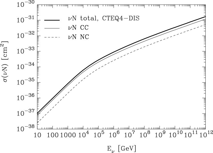
Figure 1: From Ref. Gandhi:1998ri . Cross sections for $\nu_{\ell}N$ interactions at high energies, according to the CTEQ4–DIS parton distributions: dashed line, $\sigma(\nu_{\ell}N\rightarrow\nu_{\ell}+\hbox{anything})$; thin line, $\sigma(\nu_{\ell}N\rightarrow\ell^{-}+\hbox{anything})$; thick line, total (charged-current plus neutral-current) cross section.

Imagine a neutrino of energy $E_{\nu}$ scattering on a parton $i$ carrying a fraction $x$ of the 4-momentum $P$ of a state $X$ of mass $M$. Denoting the fractional recoil energy of $X$ by $y\equiv E_{X}^{\prime}/E_{\nu}$ and the distribution of parton type $i$ by $f_{i}(x,Q)$, in the relativistic limit $E_{\nu}\gg m_{X}$ the contribution to the $\nu X$ cross section turns out to be

$$\frac{d\sigma^{\nu X}}{dxdy}=\frac{2G_{\rm F}^{2}ME_{\nu}x}{\pi}\left(\frac{M_{W,Z}^{2}}{2ME_{\nu}xy+M_{W,Z}^{2}}\right)^{2}\sum_{i}f_{i}(x,Q)\left[g_{i,L}^{2}+g_{i,R}^{2}(1-y)^{2}\right]\,.$$ (75)

Here, $g_{i,L}$ and $g_{i,R}$ are the left- and right-chiral couplings of parton $i$, respectively, given by Eq. (74). Eq. (75) applies to both charged and neutral currents, as well as to the case where $X$ represents an elementary particle such as the electron, in which case $f_{i}(x,Q)=\delta(x-1)$.

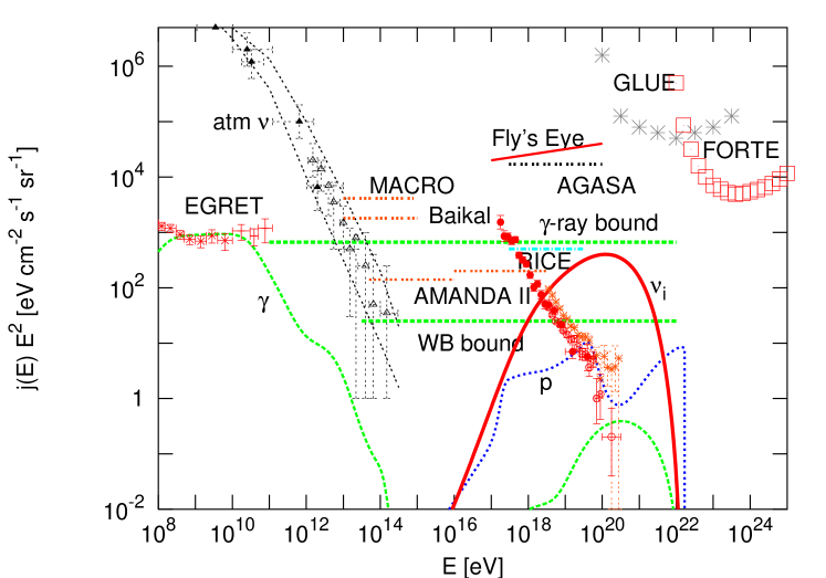
Figure 2: A scenario from Ref. ss ; dima where neutrinos are produced as secondaries of UHE cosmic rays (data with error bars above $10^{15}\,$eV) by interactions with the cosmic microwave background (CMB). Theoretical fluxes of protons, $\gamma-$rays, and neutrinos (per flavor) are as indicated. Also shown are the atmospheric neutrino flux atm-nu , as well as existing upper limits on the diffuse neutrino fluxes from MACRO MACRO , AMANDA II amandaII , BAIKAL baikal_limit , AGASA agasa_nu , the Fly’s Eye baltrusaitis and RICE rice_new experiments, and the limits obtained with the Goldstone radio telescope (GLUE) glue and the FORTE satellite forte , as indicated. The cosmic ray data are from the AGASA agasa and HiRes hires experiments To the left the newest estimate of the diffuse GeV $\gamma-$ray background from EGRET data is shown egret_new . Since most of the electromagnetic energy ends up in this energy range and since pion production produces comparable amounts of $\gamma-$rays and neutrinos, predicted neutrino fluxes cannot considerably overshoot the horizontal line on the level of the EGRET estimate marked $\gamma-$ray bound. If the sources are transparent to produced cosmic rays, the more restrictive but less general “Waxman-Bahcall bound” wb-bound , marked “WB bound”, results. This will be discussed in more detail in Sect. 9.2.

As usual, if the four-momentum transfer $Q$ becomes comparable to the electroweak scale, $Q^{2}\gg m_{W,Z}^{2}$, the weak gauge boson propagator effects, represented by the factor $M_{W,Z}^{2}/(Q^{2}+M_{W,Z}^{2})$ in Eq. (75), become important. We have used that in the limit $|Q^{2}|\gg M^{2}$ one has $0\simeq-M^{2}=(xP+Q)^{2}\simeq Q^{2}+2P\cdot Qx$ with $P\cdot Q\simeq-ME_{X}^{\prime}=-ME_{\nu}y$ evaluated in the laboratory frame, i.e. the rest frame of $X$ before the interaction. $Q^{2}\simeq 2ME_{\nu}xy$ is also called the virtuality because it is a measure for how far the exchanged gauge boson is form the mass shell $Q^{2}=-M^{2}$.

We will not derive Eq. (75) in detail, but it is easy to understand its structure: First, the overall normalization is analogous to Eq. (8), using the fact that for $E_{\nu}\gg M$ the CM momentum $p_{*}\simeq ME_{\nu}/2$. Second, if the helicities of the parton and the neutrino are equal, the total spin is zero and the scattering is spherically symmetric in the CM frame. In contrast, if the parton is right-handed, the total spin is 1 which introduces an angular dependence: After a rotation by the scattering angle $\theta_{*}$ in the CM frame the particle helicities are unchanged for the outgoing final state particle and one has to project back onto the original helicities in order to conserve spin. If a left-handed particle originally propagated along the positive z-axis, its left-handed component after scattering by $\theta_{*}$ in the $x-z$ plane is

$$\frac{1}{2}\left(1-\frac{{\hbox{\boldmath$\sigma$}}\cdot{\bf p}}{p}\right)\left(\matrix{0\cr 1}\right)=\frac{1}{2}\left(\matrix{-\sin\theta_{*}\cr 1+\cos\theta_{*}}\right)\,,$$ (76)

giving a projection $[(1+\cos\theta_{*})/2]^{2}$. Now, Lorentz transformation from the CM frame to the lab frame gives $E_{\nu}^{\prime}/E_{\nu}=(1+v_{X}\cos\theta_{*})/2\simeq(1+\cos\theta_{*})/2$ in the relativistic limit and thus the projection factor equals $(E_{\nu}^{\prime}/E_{\nu})^{2}=(1-E_{X}^{\prime}/E_{\nu})^{2}=(1-y)^{2}$, as in Eq. (75) for the right-handed parton contribution. Integrated over $0\leq y\leq 1$ this gives $1/3$, corresponding to the fact that only one of the three projections of the $J=1$ state contributes.

5.1 Neutrino-Nucleon Scattering and Applications

We now briefly consider neutrino-nucleon interaction. From Eq. (75) it is obvious that at ultra-high energies $2E_{\nu}M\gg M_{W,Z}^{2}$, the dominant contribution comes from partons with

$$x\sim\frac{M_{W,Z}^{2}}{2E_{\nu}M}\,.$$ (77)

Since, very roughly, $xf_{i}(x,Q)\propto x^{-0.3}$ for $x\ll 1$, it follows that the neutrino-nucleon cross section grows roughly $\propto E_{\nu}^{0.3}$. This is confirmed by a more detailed evaluation of Eq. (75) shown in Fig. 1.

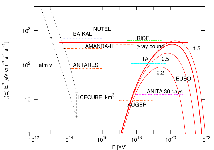
Figure 3: From Ref. ss . Similar to Fig. 2, but showing expected sensitivities of the currently being constructed Pierre Auger project to tau-neutrinos auger_nu , the planned projects Telescope Array (TA) ta_nu , the fluorescence/Čerenkov detector NUTEL mount , the space based EUSO euso_nu , the water-based Baikal baikal_limit and ANTARES antares (the NESTOR sensitivity for 1 tower would be similar to AMANDA-II and for 7 towers similar to ANTARES nestor ), the ice-based AMANDA-II amandaII and ICECUBE icecube (similar to the intended Mediterranean km³ project katz ), and the radio detectors RICE rice and ANITA anita , as indicated. All sensitivities except for ANITA and RICE refer to one year running time. For comparison, the $\gamma-$ray bound derived from the EGRET GeV $\gamma-$ray flux egret_new is also shown.

Let us use this to do a very rough estimate of event rates expected for extraterrestrial ultra-high energy (UHE) neutrinos in neutrino telescopes. Such neutrinos are usually produced via pion production by accelerated UHE protons interacting within their source or with the cosmic microwave background (CMB) during propagation to Earth. The threshold for the reaction $N\gamma\to N\pi$, for a head-on collision of a nucleon $N$ of energy $E$ with a photon of energy $\varepsilon$ is given by the condition $s=(E+\varepsilon)^{2}-\left[(E^{2}-m_{N}^{2})^{1/2}-\varepsilon\right]^{2}\geq(m_{N}+m_{\pi})^{2}$, or

$$E\geq\frac{m_{\pi}(m_{N}+m_{\pi}/2)}{2\varepsilon}\simeq 3.4\times 10^{19}\left(\frac{\varepsilon}{10^{-3}\,{\rm eV}}\right)^{-1}\,{\rm eV}\,,$$ (78)

where $\varepsilon\sim 10^{-3}\,$eV represents the energy of a typical CMB photon. At these energies, the secondary neutrino flux should therefore be very roughly comparable with the primary UHE cosmic ray flux, within large margins. Fig. 2 shows a scenario where neutrinos are produced by the primary cosmic ray interactions with the CMB. Using that the neutrino-nucleon cross section from Fig. 1 roughly scales as $\sigma_{\nu N}\propto E_{\nu}^{0.363}$ for $10^{16}\,{\rm eV}\mathrel{\mathchoice{\lower 3.6pt\vbox{\halign{$\mathsurround=0pt\displaystyle\hfil#\hfil$\cr<\crcr\sim\crcr}}}{\lower 3.6pt\vbox{\halign{$\mathsurround=0pt\textstyle\hfil#\hfil$\cr<\crcr\sim\crcr}}}{\lower 3.6pt\vbox{\halign{$\mathsurround=0pt\scriptstyle\hfil#\hfil$\cr<\crcr\sim\crcr}}}{\lower 3.6pt\vbox{\halign{$\mathsurround=0pt\scriptscriptstyle\hfil#\hfil$\cr<\crcr\sim\crcr}}}}E_{\nu}\mathrel{\mathchoice{\lower 3.6pt\vbox{\halign{$\mathsurround=0pt\displaystyle\hfil#\hfil$\cr<\crcr\sim\crcr}}}{\lower 3.6pt\vbox{\halign{$\mathsurround=0pt\textstyle\hfil#\hfil$\cr<\crcr\sim\crcr}}}{\lower 3.6pt\vbox{\halign{$\mathsurround=0pt\scriptstyle\hfil#\hfil$\cr<\crcr\sim\crcr}}}{\lower 3.6pt\vbox{\halign{$\mathsurround=0pt\scriptscriptstyle\hfil#\hfil$\cr<\crcr\sim\crcr}}}}10^{21}\,$eV, and assuming water or ice as detector medium, we obtain the rate

$$\Gamma_{\nu} \sim \sigma_{\nu N}(E_{\nu})2\pi E_{\nu}j(E_{\nu})n_{N}V_{\rm eff}$$ (79)

$$\sim 0.03\left(\frac{E_{\nu}}{10^{19}\,{\rm eV}}\right)^{-0.637}\left(\frac{E_{\nu}^{2}j(E_{\nu})}{10^{2}\,{\rm eV}{\rm cm}^{-2}{\rm sr}^{-1}{\rm s}^{-1}}\right)\left(\frac{V_{\rm eff}}{{\rm km}^{3}}\right)\,{\rm yr}^{-1}\,,$$

where $n_{N}\simeq 6\times 10^{23}\,{\rm cm}^{-3}$ is the nucleon density in water/ice, $V_{\rm eff}$ the effective detection volume, and $j(E_{\nu})$ is the differential neutrino flux in units of ${\rm cm}^{-2}{\rm eV}^{-1}{\rm sr}^{-1}{\rm s}^{-1}$.

Eq. (79) indicates that at $E_{\nu}\mathrel{\mathchoice{\lower 3.6pt\vbox{\halign{$\mathsurround=0pt\displaystyle\hfil#\hfil$\cr>\crcr\sim\crcr}}}{\lower 3.6pt\vbox{\halign{$\mathsurround=0pt\textstyle\hfil#\hfil$\cr>\crcr\sim\crcr}}}{\lower 3.6pt\vbox{\halign{$\mathsurround=0pt\scriptstyle\hfil#\hfil$\cr>\crcr\sim\crcr}}}{\lower 3.6pt\vbox{\halign{$\mathsurround=0pt\scriptscriptstyle\hfil#\hfil$\cr>\crcr\sim\crcr}}}}10^{18}\,$eV, effective volumes $\mathrel{\mathchoice{\lower 3.6pt\vbox{\halign{$\mathsurround=0pt\displaystyle\hfil#\hfil$\cr>\crcr\sim\crcr}}}{\lower 3.6pt\vbox{\halign{$\mathsurround=0pt\textstyle\hfil#\hfil$\cr>\crcr\sim\crcr}}}{\lower 3.6pt\vbox{\halign{$\mathsurround=0pt\scriptstyle\hfil#\hfil$\cr>\crcr\sim\crcr}}}{\lower 3.6pt\vbox{\halign{$\mathsurround=0pt\scriptscriptstyle\hfil#\hfil$\cr>\crcr\sim\crcr}}}}100\,{\rm km}^{3}$ are necessary. Although impractical for conventional neutrino telescopes, big air shower arrays such as the Pierre Auger experiment can achieve this. In contrast, if there are sources such as active galactic nuclei emitting at $E_{\nu}\sim 10^{16}\,$eV at a level $E_{\nu}^{2}j(E_{\nu})\sim 10^{2}\,{\rm eV}{\rm cm}^{-2}{\rm sr}^{-1}{\rm s}^{-1}$, km-scale neutrino telescopes should detect something. Such fluxes are consistent with general considerations, see Fig. 2.

Finally, Fig. 3 shows more detailed neutrino flux sensitivities expected from future experiments.

6 Dirac and Majorana Neutrinos

Up to now we have assumed that neutrinos and anti-neutrinos are separate entities. This is true if lepton number is conserved, see Tab. 1, and corresponds to pure ”Dirac neutrinos”. However, lepton number may be violated in the neutrino sector and neutrinos may be indistinguishable from anti-neutrinos. In order to elucidate this, let us first study some symmetries of the Dirac equation (27). From Eqs. (23), (25) one can easily show that

$$\gamma_{\mu}^{*}=\gamma_{2}\gamma_{\mu}\gamma_{2}\,.$$ (80)

Complex conjugating the Dirac equation (27) and multiplying it with $\xi^{*}\gamma_{2}$ from the left, it then follows that it is invariant under the ”charge conjugation transformation”

$$C\psi(x)C^{-1}\equiv\psi^{c}\equiv\xi^{*}\gamma_{2}\psi^{*}\,,$$ (81)

where $\xi$ is an arbitrary complex number with $|\xi|=1$. This transformation exchanges particles and anti-particles and satisfies $(\psi^{c})^{c}=\psi$. Note that $\gamma_{2}$ appears because according to Eq. (80) it is the only real Dirac matrix in this convention.

A Majorana neutrino satisfies the reality condition

$$\phi(x)=\gamma_{2}\phi^{*}(x)\,,\quad\mbox{or}\quad\phi^{c}=\xi^{*}\phi\,.$$ (82)

These spinors are of the form

$$\phi=\left(\matrix{-i\sigma_{2}\chi^{*}\cr\chi}\right)\,,$$ (83)

where $\chi$ is a two-spinor. This implies that for any Dirac spinor $\psi$ one can construct a Majorana spinor by

$$\phi\equiv\psi+\xi\psi^{c}\,.$$ (84)

Note that this spinor is not an eigenstate of lepton number because under a phase transformation $\psi\to\psi e^{i\alpha}$ one has $\psi^{c}\to\psi^{c}e^{-i\alpha}$. Defining

$$\psi^{c}_{L,R}\equiv(\psi^{c})_{L,R}=\frac{1\pm\gamma_{5}}{2}\psi^{c}=\left(\frac{1\mp\gamma_{5}}{2}\psi\right)^{c}\,,$$ (85)

one can define left- and right-handed Majorana fields

$$\phi_{\pm}\equiv\psi_{L,R}+(\psi_{L,R})^{c}=\psi_{L,R}+\psi_{R,L}^{c}\,.$$ (86)

Note that both these fields now contain both left and right-handed fields. What before experimentally was called neutrino and anti-neutrino now is called left- and right-handed neutrino, respectively. We can now introduce Majorana mass terms of the form

$${\cal L}_{\rm M} = -\frac{1}{2}\left(m_{L}\overline{\phi_{+}}\phi_{+}+m_{R}\overline{\phi_{-}}\phi_{-}\right)$$

$$= -\frac{1}{2}m_{L}\left(\overline{\psi_{L}}\psi_{R}^{c}+\overline{\psi_{R}^{c}}\psi_{L}\right)-\frac{1}{2}m_{R}\left(\overline{\psi_{R}}\psi_{L}^{c}+\overline{\psi_{L}^{c}}\psi_{R}\right)\,,$$

where $m_{L}$ and $m_{R}$ are real. Together with the Dirac mass term this can be written as

$${\cal L}_{\rm M}+{\cal L}_{\rm D}=-\frac{1}{2}\left(\overline{\psi_{L}},\overline{\psi_{L}^{c}}\right)\left(\matrix{m_{L}&m_{\rm D}\cr m_{\rm D}&m_{R}}\right)\left(\matrix{\psi_{R}^{c}\cr\psi_{R}}\right)+{\rm h.c.}\,,$$ (88)

where we have used $(\overline{\psi_{1}}\psi_{2})^{\dagger}=\overline{\psi_{2}}\psi_{1}$, see around Tab. 2 and (using $\gamma_{2}^{\dagger}=\gamma_{2}$ and the fact that $\psi$ anti-commutes)

$$\overline{\psi_{L}^{c}}\psi_{R}^{c} = \left[(\psi_{R})^{c}\right]^{\dagger}i\gamma^{0}\frac{1-\gamma_{5}}{2}\xi^{*}\gamma_{2}\psi^{*}=\psi_{R}^{T}\gamma_{2}^{\dagger}i\gamma^{0}\frac{1-\gamma_{5}}{2}\gamma_{2}\psi^{*}$$

$$= -i\psi_{R}^{T}\frac{1-\gamma_{5}}{2}\gamma^{0}\psi^{*}=i\left[\psi_{R}^{T}\frac{1-\gamma_{5}}{2}\gamma^{0}\psi^{*}\right]^{T}=\overline{\psi_{L}}\psi_{R}$$

for any Dirac spinors $\psi_{1,2}$ and $\psi$. Note that under $\psi\to\psi e^{i\alpha}$ Dirac terms are invariant, whereas Majorana terms pick up the phase $e^{\pm 2i\alpha}$, according to lepton number conservation and non-conservation, respectively. Furthermore, we see that for $m_{R}\gg m_{\rm D}$, $m_{L}\simeq 0$, the two mass eigenvalues in Eq. (88) are $\simeq m_{R}$ and $m_{\rm D}^{2}/m_{R}$. The latter are very small and thus may explain the sub-eV masses involved in left-chiral neutrino oscillations. This is called the see-saw mechanism which would imply that the mass eigenstates are Majorana in nature. The existence of one heavy right-handed Majorana neutrino per lepton generation is motivated by Grand Unification extensions of the electroweak gauge group to $SO(10)$ which has 16-dimensional representations that could fit 15 Standard Model lepton and quark states plus one new state, see, e.g., Ref. mohapatra .

Finally, in the exactly massless case, Dirac and Majorana particles are exactly equivalent, since the two fields Eq. (86) completely decouple, see Eq. (88). We also mention that in supersymmetric extensions of the Standard Model, the fermionic super-partners of the gauge bosons are Majorana fermions. As a consequence, they can self-annihilate which plays an important role to their being candidates for cold dark matter.

For $n>1$ neutrino flavors, mass eigenstates $\left|\nu_{i}\right>$ of mass $m_{i}$ and interaction eigenstates $\left|\nu_{\alpha}\right>$ in general are not identical, but related by a unitary $n\times n$ matrix $U$:

$$\left|\nu_{\alpha}\right>=\sum_{i}U_{\alpha i}\left|\nu_{i}\right>\,,$$ (89)

where for anti-neutrinos $U$ has to be replaced by $U^{*}$. Such a matrix in general has $n^{2}$ real parameters. Subtracting $2n-1$ relative phases of the $n$ neutrinos in the two bases, one ends up with $(n-1)^{2}$ physically independent real parameters. Of these, $n(n-1)/2$ are mixing angles, and the remaining $(n-1)(n-2)/2$ are ”$CP$-violating phases”. In order to have $CP$-violation in the Dirac neutrino sector thus requires $n\geq 3$. Once the relative phases of the different flavors have been fixed, for non-vanishing Majorana masses there will in general be $n-1$ Majorana phases that can not be projected out by $\psi\to\psi e^{i\alpha}$ in Eq. (6). Thus, the number of independent real parameters is larger, namely $n(n-1)$, in this case. Note that the corresponding Cabibbo Kobayashi Maskawa (CKM) matrix in the quark sector is pure Dirac because Majorana terms would violate electric charge conservation in the quark sector.

If at time $t=0$ a flavor eigenstate $\left|\nu_{\alpha}\right>=\sum_{i}U_{\alpha i}\left|\nu_{i}\right>$ is produced in an interaction, in vacuum the time development will thus be

$$\left|\nu(t)\right>=\sum_{i}U_{\alpha i}e^{-iE_{i}t}\left|\nu_{i}\right>=\sum_{i,\beta}U_{\alpha i}U_{\beta i}^{*}e^{-iE_{i}t}\left|\nu_{\beta}\right>\,.$$ (90)

Since masses and energies of anti-particles are equal according to the $CPT$ theorem, from this we obtain the following transition probabilities

$$P(\nu_{\alpha}\to\nu_{\beta}) = \left|\sum_{i}U_{\alpha i}U^{*}_{\beta i}\exp(-iE_{i}t)\right|^{2}$$

$$P(\bar{\nu}_{\alpha}\to\bar{\nu}_{\beta}) = \left|\sum_{i}U^{*}_{\alpha i}U_{\beta i}\exp(-iE_{i}t)\right|^{2}\,.$$ (91)

From this follows immediately

$$P(\nu_{\alpha}\to\nu_{\beta})=P(\bar{\nu}_{\beta}\to\bar{\nu}_{\alpha})\,,$$ (92)

which is due to the $CPT$ theorem. Furthermore, if the mixing matrix satisfies a reality condition of the form

$$U_{\alpha i}=U^{*}_{\alpha i}\eta_{i}\,,$$ (93)

with $\eta_{i}$ phases, corresponding to $CP$-conservation, one also has

$$P(\nu_{\alpha}\to\nu_{\beta})=P(\bar{\nu}_{\alpha}\to\bar{\nu}_{\beta})\,.$$ (94)

We mention two other important differences between Dirac and Majorana neutrinos:

• Neutrino-less double beta-decay is only possible in the presence of Majorana masses because the final state $e^{-}e^{-}$ violates lepton number. In this case the rate is proportional to the square of

  $$m_{ee}=\left|\sum_{i}|U_{ei}|^{2}m_{i}e^{i\alpha_{i}}\right|\,,$$ (95)

  see Eq. (88), where only one of the Majorana phases $\alpha_{i}$ can be projected out. Apart from these phases, this equation results from Eq. (90) for $\alpha=\beta=e$. There is even evidence claimed for this kind of decay, and thus for an electron neutrino Majorana mass around 0.4 eV, see Ref. klapdor . The issue is expected to be settled by next generation experiments such as CUORE cuore .

  In contrast, in $\beta-$decay with neutrinos, the electron spectra are influenced by the individual eigenstates of real mass $m_{i}$, and not by any phases. The current best experimental upper limit is given by the Mainz experiment based on tritium $\beta-$decay ${}^{3}{\rm H}\to^{3}{\rm He}e^{-}\bar{\nu}_{e}$ mainz ,

  $$m_{\nu_{e}}=\sqrt{\sum_{i}|U_{ei}|^{2}m^{2}_{i}}\mathrel{\mathchoice{\lower 3.6pt\vbox{\halign{$\mathsurround=0pt\displaystyle\hfil#\hfil$\cr<\crcr\sim\crcr}}}{\lower 3.6pt\vbox{\halign{$\mathsurround=0pt\textstyle\hfil#\hfil$\cr<\crcr\sim\crcr}}}{\lower 3.6pt\vbox{\halign{$\mathsurround=0pt\scriptstyle\hfil#\hfil$\cr<\crcr\sim\crcr}}}{\lower 3.6pt\vbox{\halign{$\mathsurround=0pt\scriptscriptstyle\hfil#\hfil$\cr<\crcr\sim\crcr}}}}2.2\,{\rm eV}$$ (96)

  at 95% confidence level (CL). The KATRIN experiment katrin aims at a sensitivity down to $0.2\,$eV within the next few years.

• Majorana neutrinos cannot have magnetic dipole moments between equal neutrino flavors, as seen from the following identity using Eqs. (82), (80), (34), and the reality of the spinors in Tab. 2:

  $$i\overline{\psi_{1}}[\gamma_{\mu},\gamma_{\nu}]\psi_{2}=-\psi_{1}^{T}\gamma_{2}\gamma^{0}[\gamma_{\mu},\gamma_{\nu}]\gamma_{2}\psi_{2}^{*}=-\psi_{1}^{T}\left(\gamma^{0}[\gamma_{\mu},\gamma_{\nu}]\right)^{*}\psi_{2}^{*}=$$

  $$=-\left(\psi_{1}^{\dagger}\gamma^{0}[\gamma_{\mu},\gamma_{\nu}]\psi_{2}\right)^{*}=\left(\psi_{1}^{\dagger}\gamma^{0}[\gamma_{\mu},\gamma_{\nu}]\psi_{2}\right)^{\dagger}=-i\overline{\psi_{2}}[\gamma_{\mu},\gamma_{\nu}]\psi_{1}\,,$$

  where in the second-last identity we have used that transposition changes the order of the fermionic fields, thus picking up a minus sign. As a consequence, only transition magnetic moments between different flavors are possible for Majorana neutrinos.

7 Neutrino Oscillations

Let us now restrict to two-neutrino oscillations, $n=2$, between $\left|\nu_{e}\right>$ and $\left|\nu_{\mu}\right>$, say, and write

$$U=\left(\matrix{\cos\theta_{0}&\sin\theta_{0}\cr-\sin\theta_{0}&\cos\theta_{0}}\right)$$ (97)

for the mixing matrix in Eq. (89) which is characterized by one real vacuum mixing angle $\theta_{0}$. Since $id\left|\nu_{i}\right>/dt=E_{i}\left|\nu_{i}\right>$ for $i=1,2$ in the mass basis, and since $E_{i}=(m_{i}^{2}+p^{2})^{1/2}\simeq p+m_{i}^{2}/(2p)\simeq E+m_{i}^{2}/(2E)$ in the relativistic limit $p\gg m_{i}$, using the trigonometric identities $\cos^{2}\theta_{0}-\sin^{2}\theta_{0}=\cos 2\theta_{0}$, $2\cos\theta_{0}\sin\theta_{0}=\sin 2\theta_{0}$, it follows from Eqs. (89), (97) that

$$i\frac{d}{dt}\left(\matrix{\nu_{e}\cr\nu_{\mu}}\right)_{E}=\left[\left(E+\frac{m_{1}^{2}+m_{2}^{2}}{4E}\right)+\frac{\Delta m^{2}}{4E}\left(\matrix{\cos 2\theta_{0}&-\sin 2\theta_{0}\cr-\sin 2\theta_{0}&-\cos 2\theta_{0}}\right)\right]\left(\matrix{\nu_{e}\cr\nu_{\mu}}\right)_{E}\,,$$ (98)

where we consider a given momentum mode ${\bf p}$, and $\Delta m^{2}\equiv m_{1}^{2}-m_{2}^{2}$. From now on we will consider the relativistic limit with $p\simeq E$. The first term in Eq. (98) is a common phase factor and can be ignored.

The integrated version of this is Eq. (90). Then applying Eq. (91), one can show that this has the solution

$$P(\nu_{\alpha}\to\nu_{\beta})=\frac{1}{2}\sin^{2}2\theta_{0}\left(1-\cos\Delta m^{2}\frac{L}{2E}\right)\,\quad\mbox{for}\quad\alpha\neq\beta\,,$$ (99)

for oscillations over a length $L$. The oscillation length in vacuum is thus

$$L_{0}=4\pi\frac{E}{|\Delta m^{2}|}\simeq 2.48\,\left(\frac{E}{{\rm MeV}}\right)\left(\frac{|\Delta m^{2}|}{{\rm eV}^{2}}\right)^{-1}\,{\rm m}\,.$$ (100)

Neutrino oscillations are modified by forward scattering amplitudes in matter. Since neutral currents are by definition flavor-neutral, they only contribute to the common phase factor which in the following will be ignored. The charged current interaction is diagonal in flavor space and, according to Eqs. (68), (69), and (71), the low-energy limit of its forward scattering part for $\nu_{e}({\bf p})$ has the form

$$2\sqrt{2}G_{\rm F}\sum_{{\bf p}^{\prime}}\left[e({\bf p}^{\prime})^{\dagger}\gamma^{0}\gamma^{\mu}\frac{1+\gamma_{5}}{2}\nu_{e}({\bf p})\right]\left[\nu_{e}({\bf p})^{\dagger}\gamma^{0}\gamma_{\mu}\frac{1+\gamma_{5}}{2}e({\bf p}^{\prime})\right]\,,$$ (101)

where we have used $\bar{\psi}=\psi^{\dagger}i\gamma^{0}$. We need to express this in terms of Dirac bilinears of the form Tab. 2 for electrons and neutrinos separately. In order to do that we use the fact that every $4\times 4$ matrix ${\cal O}$ can be expanded according to

$${\cal O}=\sum_{i}\frac{{\rm tr}({\cal O}{\cal O}_{i})}{{\rm tr}({\cal O}_{i}^{2})}{\cal O}_{i}\,,$$ (102)

where ${\cal O}_{i}$ are the 16 matrices appearing in Tab. 2 which satisfy ${\rm tr}({\cal O}_{i}{\cal O}_{j})=0$ for $i\neq j$. Using this one can show that

$$\left(\gamma^{0}\gamma^{\mu}\frac{1+\gamma_{5}}{2}\right)_{\alpha\beta}\left(\gamma^{0}\gamma_{\mu}\frac{1+\gamma_{5}}{2}\right)_{\gamma\delta}=$$

$$\left(\frac{1+\gamma_{5}}{2}\right)_{\gamma\beta}\left(\frac{1+\gamma_{5}}{2}\right)_{\alpha\delta}+\frac{1}{8}\left(\left[\gamma^{\lambda},\gamma^{\kappa}\right]\frac{1+\gamma_{5}}{2}\right)_{\gamma\beta}\left(\left[\gamma_{\lambda},\gamma_{\kappa}\right]\right)_{\alpha\delta}\,.$$ (103)

Applying this to Eq. (101) and noting that the last term in Eq. (103) does not contribute in the rest frame of the electron plasma, one obtains

$$-2\sqrt{2}G_{\rm F}\left[\nu_{e}({\bf p})^{\dagger}\frac{1+\gamma_{5}}{2}\nu_{e}({\bf p})\right]\sum_{{\bf p}^{\prime}}\left[e({\bf p}^{\prime})^{\dagger}\frac{1+\gamma_{5}}{2}e({\bf p}^{\prime})\right]\,,$$ (104)

where we have picked up an extra minus from the anti-commutation of fermionic fields. The electron and neutrino fields have the form Eq. (17). The matter-dependent part of the sum in Eq. (104) thus takes the form $\sum_{\bf p}(a_{e,L}^{\dagger}({\bf p})a_{e,L}({\bf p})-b_{e,L}^{\dagger}({\bf p})b_{e,L}({\bf p})$. When tracing out the charged lepton density matrix, this reduces to the density of left-chiral electrons minus the density of left-chiral positrons. Thus, for an unpolarized plasma, the contribution to the $\left|\nu_{e}\right>$ self-energy finally is $-\sqrt{2}G_{\rm F}N_{e}$, where $N_{e}$ is the electron-number density, i.e. the electron minus the positron density, and analogously for the other active flavors. The non-trivial part of Eq. (98) is thus modified to

$$i\frac{d}{dt}\left(\matrix{\nu_{e}\cr\nu_{\mu}}\right)_{E}=\left(\matrix{\frac{\Delta m^{2}\cos 2\theta_{0}}{4E}-\sqrt{2}G_{\rm F}N_{e}&-\frac{\Delta m^{2}\sin 2\theta_{0}}{4E}\cr-\frac{\Delta m^{2}\sin 2\theta_{0}}{4E}&-\frac{\Delta m^{2}\cos 2\theta_{0}}{4E}-\sqrt{2}G_{\rm F}N_{\mu}}\right)\left(\matrix{\nu_{e}\cr\nu_{\mu}}\right)_{E}\,.$$ (105)

It is illustrative to write this in terms of the hermitian density matrix $\rho_{\bf p}(t)\equiv\left.|\nu_{\bf p}(t)\right\rangle\left\langle\nu_{\bf p}(t)\right.|$. If we expand this into an occupation number $n_{\bf p}$ and polarization ${\bf P_{p}}$, $\rho_{\bf p}=\frac{1}{2}\left(n_{\bf p}+{\bf P_{p}}\cdot{\hbox{\boldmath$\sigma$}}\right)$, one can easily show that Eq. (105) is equivalent to

$$\dot{\bf P}_{\bf p}={\bf B_{p}}\times{\bf P_{p}}\,,$$ (106)

where the precession vector ${\bf B_{p}}\equiv{\bf B}({\bf p})$

$$B_{1}({\bf p}) = \frac{\Delta m^{2}}{2E}\sin 2\theta_{0}\,,$$

$$B_{3}({\bf p}) = \frac{\Delta m^{2}}{2E}\cos 2\theta_{0}-\sqrt{2}G_{\rm F}N\,,$$ (107)

where $N=N_{e}-N_{\mu,\tau}$ for $\nu_{e}-\nu_{\mu,\tau}$ mixing and $N=N_{e,\mu,\tau}-N_{n}$ for active-sterile mixing, with $N_{n}$ a combination of nucleon densities. Thus, neutrino oscillations are mathematically equivalent to the precession of a magnetic moment in a variable external magnetic field.

Eq. 107) shows immediately that at the resonance density

$$N_{r}\equiv\frac{\Delta m^{2}\cos 2\theta_{0}}{2\sqrt{2}G_{\rm F}E}$$ (108)

the two diagonal entries in Eq. (105) become equal or, equivalently, $B_{3}({\bf p})=0$. More generally, Eqs. (105), (106), (107) are diagonalized by a mixing matrix Eq. (97) where $\theta_{0}$ is replaced by the mixing angle in matter $\theta_{E}$ given by

$$\tan 2\theta_{E}=\frac{\tan 2\theta_{0}}{1-N/N_{r}}\,.$$ (109)

Maximum mixing, $\theta_{E}=\pi/4$, thus occurs at the so-called Michaev-Smirnow-Wolfenstein (MSW) resonance at $N=N_{r}$. For $N\ll N_{r}$ one thus has vacuum mixing, $\theta_{E}\simeq\theta_{0}$, whereas for $N\gg N_{r}$ one has $\theta_{E}\ll\theta_{0}$. Eq. (106) now shows that propagation from $N\gg N_{r}$ to $N\ll N_{r}$ can lead to an efficient transition from one flavor to another, as long as $|\dot{\bf B}_{\bf p}|\mathrel{\mathchoice{\lower 3.6pt\vbox{\halign{$\mathsurround=0pt\displaystyle\hfil#\hfil$\cr<\crcr\sim\crcr}}}{\lower 3.6pt\vbox{\halign{$\mathsurround=0pt\textstyle\hfil#\hfil$\cr<\crcr\sim\crcr}}}{\lower 3.6pt\vbox{\halign{$\mathsurround=0pt\scriptstyle\hfil#\hfil$\cr<\crcr\sim\crcr}}}{\lower 3.6pt\vbox{\halign{$\mathsurround=0pt\scriptscriptstyle\hfil#\hfil$\cr<\crcr\sim\crcr}}}}|{\bf B_{p}}|^{2}$. Such transitions are called adiabatic. Note that since masses of anti-particles and particles are equal, whereas the lepton numbers $N_{e,\mu,\tau}$ change sign under charge conjugation, resonances in matter occur either for neutrinos or for anti-neutrinos.

In subsequent sections we will apply this to various observational evidence for neutrino oscillations.

8 Selected Applications in Astrophysics and Cosmology

8.1 Stellar Burning and Solar Neutrino Oscillations

Weak interactions are crucial in cosmology and stellar physics. In main sequence stars the first stage of hydrogen fusion into helium is the weak interaction

$$p+p\to\mbox{${}^{2}$H}+e^{+}+\nu_{e}\,.$$ (110)

The subsequent reactions ²H$+p\to^{3}$He$+\gamma$ and ³He$+^{3}$He$\to^{4}$He$+p+p$ lead to the net reaction

$$4p\to\mbox{${}^{4}$He}+2e^{+}+2\nu_{e}+26.73\,{\rm MeV}\,.$$ (111)

For many more details see Ref. raffelt .

When normalized to the solar energy flux arriving at Earth, one can calculate the expected neutrino fluxes within the so-called Standard Solar Model. The resulting fluxes in this “pp” channel as well as in other reaction channels are shown in Fig. 4

Figure 4: The predicted solar neutrino energy spectrum from Ref. bp04 . For continuum sources, the neutrino fluxes are given in number per ${\rm cm^{-2}sec^{-1}MeV^{-1}}$ at the Earth’s surface. For line sources, the units are number per ${\rm cm^{-2}sec^{-1}}$. The total theoretical uncertainties are shown. The CNO neutrino fluxes are not shown.

However, less than half of the expected solar electron-neutrino flux at a few MeV has been observed. On the other hand, neutral current experiments with the Sudbury Neutrino Observatory (SNO) sno have shown that the sum of the electron, muon- and tau neutrino flux coincides with the expected electron neutrino flux. This can be explained by an MSW transition of $\nu_{e}$ into $\nu_{\mu}$ and $\nu_{\tau}$ within the Sun with a $\Delta m^{2}_{\rm solar}\sim 10^{-5}\,{\rm eV}^{2}$. Note that this corresponds to a vacuum oscillation length Eq. (100) of a few hundred kilometers. Recently this has been confirmed independently by the KamLAND experiment kamland which measured the disappearance of the $\bar{\nu}_{e}$ neutrinos produced by nuclear reactors a few hundred kilometers from the detector. The best fit parameters for the parameters of mixing of two neutrinos in vacuum from all solar and reactor data are bahcall

$$\Delta m^{2}_{\rm solar}\simeq 8.2^{+0.3}_{-0.3}(^{+1.0}_{-0.8})\times 10^{-5}\,{\rm eV}^{2}\,;\quad\tan^{2}\theta_{\rm solar}\simeq 0.39^{+0.05}_{-0.04}(^{+0.19}_{-0.11})\,,$$ (112)

where $1\sigma$ and $3\sigma$ errors are given. The relevant contour plots are shown in Fig. 5. It is interesting to note that maximal mixing is strongly excluded, $\tan\theta_{\rm solar}\leq 1.0$ at $5.8\sigma$.

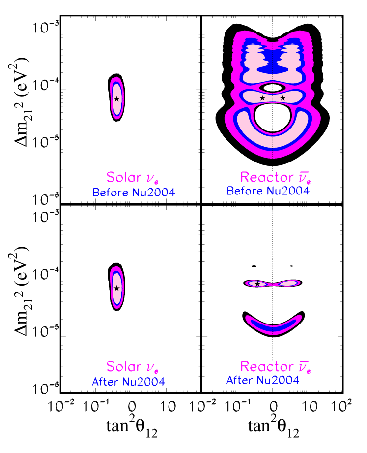
Figure 5: From Ref. bahcall . Allowed oscillation parameters: Solar vs KamLAND. The two left panels show the 90%, 95%, 99%, and 3$\sigma$ allowed regions for oscillation parameters that are obtained by a global fit of all the available solar data. The two right panels show the 90%, 95%, 99%, and 3$\sigma$ allowed regions for oscillation parameters that are obtained by a global fit of all the reactor data from KamLAND and CHOOZ. The two upper (lower) panels correspond to the analysis of all data available before (after) the Neutrino 2004 conference, June 14-19, 2004 (Paris). The new KamLAND data are sufficiently precise that matter effects discernibly break the degeneracy between the two mirror vacuum solutions in the lower right panel.

Finally, since solar and reactor neutrino experiments deal with $\nu_{e}$ and $\bar{\nu}_{e}$, respectively, comparison of the two corresponding oscillations parameters allows to set limits on $CPT$-violation in the neutrino sector.

8.2 Atmospheric Neutrinos

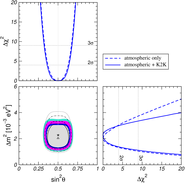
Figure 6: From Ref. maltoni . Allowed ($\sin^{2}\theta_{\rm atmos}$, $\Delta m^{2}_{\rm atmos}$) regions at 90%, 95%, 99%, and 3$\sigma$ CL for two degrees of freedom. The regions delimited by the lines correspond to atmospheric data only, while for the colored regions also K2K data are added. The best fit point of atmospheric (atmospheric + K2K) data is marked by a triangle (star). Also shown is the $\Delta\chi^{2}$ as a function of $\sin^{2}\theta_{\rm atmos}$ and $\Delta m^{2}_{\rm atmos}$, minimized with respect to the undisplayed parameter.

Cosmic rays interact in the atmosphere and produce, among other particles, pions and kaons whose decay products contain neutrinos. The observed ratio of upcoming to down-going atmospheric muon neutrinos is about 0.5 in the GeV range. Since upcoming neutrinos travel several thousand kilometers, this can be interpreted as vacuum oscillations between muon and tau-neutrinos. The best fit parameters are

$$\Delta m^{2}_{\rm atmos}\simeq 2.1\times 10^{-3}\,{\rm eV}^{2}\,;\quad\sin^{2}\theta_{\rm atmos}\simeq 0.5\,,$$ (113)

consistent with maximal mixing. The corresponding contours resulting from atmospheric and long baseline neutrino oscillation data from K2K k2k are shown in Fig. 6. Recently, the $L/E$ dependence, see Eq. (99), characteristic for neutrino oscillations has been confirmed by the Superkamiokande experiment superk , thereby strongly constraining alternative explanations of muon neutrino disappearance such as neutrino decay ashie . In addition, oscillations into sterile neutrinos are strongly disfavored over oscillations into tau-neutrinos via the following discriminating effects: Neutral currents would be non-diagonal for oscillations into sterile states, thus modifying oscillation amplitudes and total scattering rates, and charged current interactions of tau-neutrinos imply $\tau$ appearance.

In 3-neutrino oscillation schemes $\theta_{\rm solar}$ and $\theta_{\rm atmos}$ are usually identified with $\theta_{12}$ and $\theta_{23}$, respectively (we here assume the “normal mass hierarchy” $m_{1},m_{2}\ll m_{3}$ which seems the most natural for neutrino mass modeling in Grand Unification scenarios altarelli ). According to the discussion around Eq. (89), there is one more mixing angle $\theta_{13}$ and at least one Dirac $CP$-violating phase called $\delta$. Note that solar and atmospheric neutrinos only decouple exactly for $\theta_{13}=0$ in which case $CP$ would also be conserved. Whereas there are at most weak indications for leptonic $CP$-violations yet klinkhamer , the third mixing angle is constrained at 3$\sigma$ CL by Ref. maltoni

$$\sin^{2}\theta_{13}\leq 0.061\,.$$ (114)

We finally stress that neutrino oscillations are sensitive only to differences of squared masses, not to absolute mass scales. To probe the latter requires laboratory experiments discussed earlier such as $\beta-$decay, the study of cosmological effects such as the influence of neutrino mass on the power spectrum, see Sect. 8.4, or measuring time delays of astrophysical neutrino bursts from $\gamma-$ray bursts and supernovae relative to the speed of light.

8.3 Big Bang Nucleosynthesis (BBN)

For more detailed introductions to the following three topics we refer the reader to standard text books kt ; mohapatra .

The early universe consisted of a mixture of protons, neutrons, electrons, positrons, photons and neutrinos. Their relative abundances were determined by thermodynamic equilibrium until the weak interactions ”froze out” once the temperature of the expanding universe dropped below $T_{f}\sim 1\,$MeV where their rates became smaller than the expansion rate. For example, according to Eqs. (7) and (8) the interaction rates of nucleons $\overline{\nu}_{e}p\leftrightarrow ne^{+}$ and $e^{-}p\leftrightarrow n\nu_{e}$ are

$$\Gamma\sim n\sigma\propto G_{\rm F}^{2}T^{5}$$ (115)

at temperatures $100\,{\rm GeV}\mathrel{\mathchoice{\lower 3.6pt\vbox{\halign{$\mathsurround=0pt\displaystyle\hfil#\hfil$\cr>\crcr\sim\crcr}}}{\lower 3.6pt\vbox{\halign{$\mathsurround=0pt\textstyle\hfil#\hfil$\cr>\crcr\sim\crcr}}}{\lower 3.6pt\vbox{\halign{$\mathsurround=0pt\scriptstyle\hfil#\hfil$\cr>\crcr\sim\crcr}}}{\lower 3.6pt\vbox{\halign{$\mathsurround=0pt\scriptscriptstyle\hfil#\hfil$\cr>\crcr\sim\crcr}}}}T\mathrel{\mathchoice{\lower 3.6pt\vbox{\halign{$\mathsurround=0pt\displaystyle\hfil#\hfil$\cr>\crcr\sim\crcr}}}{\lower 3.6pt\vbox{\halign{$\mathsurround=0pt\textstyle\hfil#\hfil$\cr>\crcr\sim\crcr}}}{\lower 3.6pt\vbox{\halign{$\mathsurround=0pt\scriptstyle\hfil#\hfil$\cr>\crcr\sim\crcr}}}{\lower 3.6pt\vbox{\halign{$\mathsurround=0pt\scriptscriptstyle\hfil#\hfil$\cr>\crcr\sim\crcr}}}}1\,$MeV where the neutron-proton mass difference $m_{n}-m_{p}=1.293\,$MeV and the electron mass are negligible and the $e^{\pm}$ and electron neutrino densities $n\sim T^{3}$. This becomes indeed comparable to the expansion rate

$$H\sim\rho^{1/2}/m_{\rm P}\sim g_{*}^{1/2}T^{2}/m_{\rm P}\,,$$ (116)

where $\rho$ is the total energy density and $g_{*}$ the number of relativistic degrees of freedom, once $T$ approaches $T_{f}\simeq 1\,$MeV. The equilibrium neutron to proton ratio at that temperature is given by thermodynamics as

$$\frac{n_{n}}{n_{p}}=\exp\left[-(m_{n}-m_{p})/T_{f}\right]$$ (117)

At that time, the free neutrons were quickly bound into helium which could not be broken up any more by the cooling thermal radiation. The helium abundance was thus determined by the freeze out of electroweak interactions. Since equating Eq. (115) with Eq. (116) yields $T_{f}\propto g_{*}^{1/6}$ we also see that the helium abundance should increase with $g_{*}$. Since the number $N_{\nu}$ of stable neutrino species with mass below $\sim 1\,$MeV contributes to $g_{*}$, this number is constrained by the observed helium abundance. More generally, in the absence of a significant asymmetry between neutrinos and anti-neutrinos, elemental abundances depend only on the effective number of relativistic neutrinos $N_{\nu}$ and the baryon to photon ratio

$$\eta_{10}\equiv 10^{10}\frac{n_{B}}{n_{\gamma}}\,.$$ (118)

Predictions for standard big bang nucleosynthesis (SBBN) with $N_{\nu}=3$, the number of active neutrinos consistent with the $Z$ boson width, are shown in Fig. 7. A detailed comparison of measured and predicted abundances shown in Fig. 7 with $\eta_{10}$ and $N_{\nu}$ free parameters yields the following: The universal density of baryons $\eta_{10}$ inferred from SBBN and the measured deuterium abundance, $\eta_{10}({\rm SBBN})=6.10^{+0.67}_{-0.52}$, is in excellent agreement with the baryon density derived largely from CMB data spergel , $\eta_{10}({\rm CMB})=6.14\pm 0.25$. However, there is a $\simeq 2\sigma$ tension between the ⁴He abundance predicted by SBBN with this concordance $\eta_{10}$ and the observed one. This tension can be mitigated if $N_{\nu}$ is allowed to be smaller than the canonical $N_{\nu}=3$. If both the baryon density $\eta_{10}$ and $N_{\nu}$, or equivalently, the expansion rate, are allowed to be free parameters, BBN (D, ³He, and ⁴He) and the CMB (WMAP) agree at 95% CL for $5.5\leq\eta_{10}\leq 6.8$ ($0.020\leq\Omega_{\rm B}h^{2}\leq 0.025$ for the baryon density in terms of the critical density) and $1.65\leq$ N${}_{\nu}\leq 3.03$ steigman . Are these hints for new physics ?

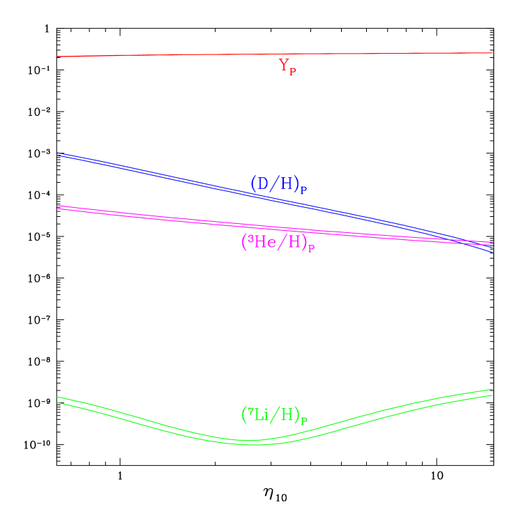
Figure 7: From Ref. steigman . The SBBN-predicted primordial abundances of D, ³He, and ⁷Li by number with respect to hydrogen, and the ⁴He mass fraction Y_P, as a function of the nucleon (baryon) abundance parameter $\eta_{10}$. The bands reflect the theoretical uncertainties ($\pm 1\sigma$) in the BBN predictions.

8.4 Neutrino Hot Dark Matter

Finally, massive neutrinos in the eV range contribute to the density of non-relativistic matter in today’s universe,

$$\Omega_{\nu}h^{2}=\frac{\sum m_{\nu}}{92.5\,{\rm eV}}$$ (119)

in terms of the critical (closure) density for $m_{\nu}\gg 10^{-4}\,$eV, today’s temperature. Eq. (119) results from the fact that neutrinos have been relativistic at decoupling at $T\sim 1\,$MeV, thus constituting hot dark matter, and their number density is simply determined by the redshifted number density at freeze-out, in analogy to Sect. 8.3.

Since neutrinos are freely streaming on scales of many Mpc, the matter power spectrum is reduced by a relative amount $\Delta P_{m}/P_{m}=-8\Omega_{\nu}/\Omega_{m}$, where $\Omega_{m}$ is the total matter density. A combination of data on the large scale structure and the CMB then leads to the limit hannestad

$$\sum m_{\nu}\mathrel{\mathchoice{\lower 3.6pt\vbox{\halign{$\mathsurround=0pt\displaystyle\hfil#\hfil$\cr<\crcr\sim\crcr}}}{\lower 3.6pt\vbox{\halign{$\mathsurround=0pt\textstyle\hfil#\hfil$\cr<\crcr\sim\crcr}}}{\lower 3.6pt\vbox{\halign{$\mathsurround=0pt\scriptstyle\hfil#\hfil$\cr<\crcr\sim\crcr}}}{\lower 3.6pt\vbox{\halign{$\mathsurround=0pt\scriptscriptstyle\hfil#\hfil$\cr<\crcr\sim\crcr}}}}1.0\,{\rm eV}\,.$$ (120)

There was even a claim for a positive detection with allen

$$\sum m_{\nu}\simeq 0.56\,{\rm eV}\,,$$ (121)

but newest analyses suggest upper bounds even slightly below this lya .

It is intriguing that direct experimental bounds Eq. (96) and cosmological bounds Eq. (120) have reached comparable sensitivities. In addition, both a combination of future CMB data from the Planck satellite with large scale structure surveys hannestad and next generation laboratory experiments such as KATRIN will probe the 0.1 eV regime.

Assuming three active neutrino oscillations with the parameters discussed in Sects. 8.1 and 8.2 has an interesting cosmological consequence: Flavor equilibrium is reached before the BBN epoch and the asymmetry parameter $\xi_{\nu}=\mu_{\nu}/T$, where $\mu_{\nu}$ is the common neutrino chemical potential, is constrained by dhpprs

$$\left|\xi_{\nu}\right|\mathrel{\mathchoice{\lower 3.6pt\vbox{\halign{$\mathsurround=0pt\displaystyle\hfil#\hfil$\cr<\crcr\sim\crcr}}}{\lower 3.6pt\vbox{\halign{$\mathsurround=0pt\textstyle\hfil#\hfil$\cr<\crcr\sim\crcr}}}{\lower 3.6pt\vbox{\halign{$\mathsurround=0pt\scriptstyle\hfil#\hfil$\cr<\crcr\sim\crcr}}}{\lower 3.6pt\vbox{\halign{$\mathsurround=0pt\scriptscriptstyle\hfil#\hfil$\cr<\crcr\sim\crcr}}}}0.07\,.$$ (122)

As a consequence, neutrino degeneracy is unobservable in the large scale structure and the CMB.

8.5 Leptogenesis and Baryogenesis

Neutrino masses may also play a key role in explaining the fact that we live in a universe dominated by matter rather than anti-matter. The heavy right-handed Majorana neutrinos involved in the seesaw mechanism discussed in Sect. 6 could have been produced in the early Universe and their out-of-equilibrium decays could give rise to a non-vanishing net lepton number $L$. Non-perturbative quantum effects related to the non-abelian character of the electroweak interactions can translate this into a net baryon number $B$ while conserving $B-L$. The amount of baryon number $n_{B}$ created in this scenario is related to the low-energy leptonic $CP$-violation phase $\delta$ buchmueller . Its compatibility with the observed value for the baryon per photon number $n_{B}/n_{\gamma}\simeq 6\times 10^{-10}$ implies a lower bound $m_{R}\mathrel{\mathchoice{\lower 3.6pt\vbox{\halign{$\mathsurround=0pt\displaystyle\hfil#\hfil$\cr>\crcr\sim\crcr}}}{\lower 3.6pt\vbox{\halign{$\mathsurround=0pt\textstyle\hfil#\hfil$\cr>\crcr\sim\crcr}}}{\lower 3.6pt\vbox{\halign{$\mathsurround=0pt\scriptstyle\hfil#\hfil$\cr>\crcr\sim\crcr}}}{\lower 3.6pt\vbox{\halign{$\mathsurround=0pt\scriptscriptstyle\hfil#\hfil$\cr>\crcr\sim\crcr}}}}{\rm few}\,10^{10}\,$GeV. Via the see-saw relation $m_{\nu}\simeq m_{D}^{2}/m_{R}$ for the light neutrino mass, this corresponds to an optimal range $10^{-3}\,{\rm eV}\mathrel{\mathchoice{\lower 3.6pt\vbox{\halign{$\mathsurround=0pt\displaystyle\hfil#\hfil$\cr<\crcr\sim\crcr}}}{\lower 3.6pt\vbox{\halign{$\mathsurround=0pt\textstyle\hfil#\hfil$\cr<\crcr\sim\crcr}}}{\lower 3.6pt\vbox{\halign{$\mathsurround=0pt\scriptstyle\hfil#\hfil$\cr<\crcr\sim\crcr}}}{\lower 3.6pt\vbox{\halign{$\mathsurround=0pt\scriptscriptstyle\hfil#\hfil$\cr<\crcr\sim\crcr}}}}m_{\nu}\mathrel{\mathchoice{\lower 3.6pt\vbox{\halign{$\mathsurround=0pt\displaystyle\hfil#\hfil$\cr<\crcr\sim\crcr}}}{\lower 3.6pt\vbox{\halign{$\mathsurround=0pt\textstyle\hfil#\hfil$\cr<\crcr\sim\crcr}}}{\lower 3.6pt\vbox{\halign{$\mathsurround=0pt\scriptstyle\hfil#\hfil$\cr<\crcr\sim\crcr}}}{\lower 3.6pt\vbox{\halign{$\mathsurround=0pt\scriptscriptstyle\hfil#\hfil$\cr<\crcr\sim\crcr}}}}0.1\,$eV, in remarkable agreement with the observed atmospheric and solar neutrino mass scales buchmueller . In general baryogenesis requires violation of baryon number $B$, charge conjugation $C$, combined charge and parity conjugation $CP$, and a departure from thermal equilibrium, usually caused by the expansion of the Universe. These conditions are known as the Sakharov conditions sakharov . For more details see Refs. mohapatra and kt .

9 Ultra-High Energy Cosmic Radiation

In the final part we discuss some current theoretical issues around ultra-high energy cosmic rays, $\gamma-$rays and neutrinos. We will see how some of the topics discussed in the previous two parts play an important role in this subject.

9.1 Introduction

High energy cosmic ray (CR) particles are shielded by Earth’s atmosphere and reveal their existence on the ground only by indirect effects such as ionization and showers of secondary charged particles covering areas up to many km² for the highest energy particles. In fact, in 1912 Victor Hess discovered CRs by measuring ionization from a balloon hess , and in 1938 Pierre Auger proved the existence of extensive air showers (EAS) caused by primary particles with energies above $10^{15}\,$eV by simultaneously observing the arrival of secondary particles in Geiger counters many meters apart auger_disc .

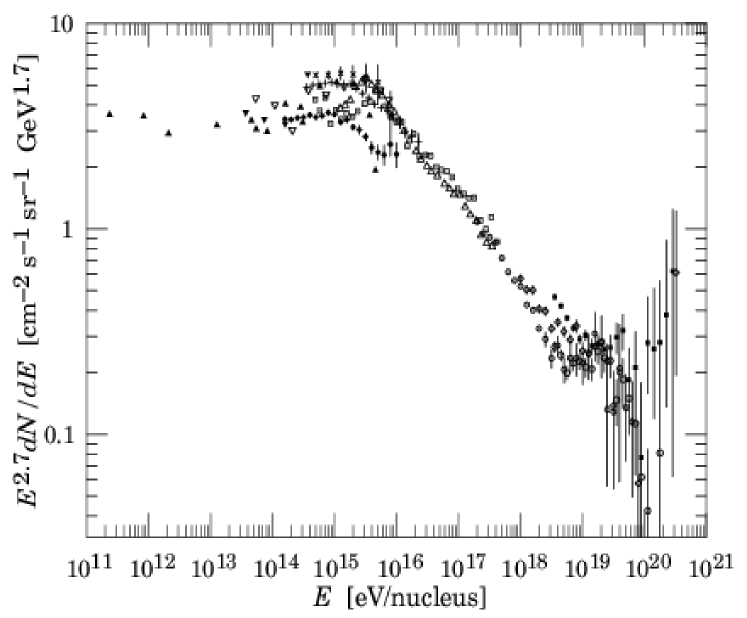
Figure 8: From Ref. rpp . The cosmic ray all particle spectrum.

After almost 90 years of research, the origin of cosmic rays is still an open question, with a degree of uncertainty increasing with energy crbook : Only below 100 MeV kinetic energy, where the solar wind shields protons coming from outside the solar system, the sun must give rise to the observed proton flux. Above that energy the CR spectrum exhibits little structure and is approximated by broken power laws $\propto E^{-\gamma}$: At the energy $E\simeq 4\times 10^{15}\,$eV called the “knee”, the flux of particles per area, time, solid angle, and energy steepens from a power law index $\gamma\simeq 2.7$ to one of index $\simeq 3.0$. The bulk of the CRs up to at least that energy is believed to originate within the Milky Way Galaxy, typically by shock acceleration in supernova remnants. The spectrum continues with a further steepening to $\gamma\simeq 3.3$ at $E\simeq 4\times 10^{17}\,$eV, sometimes called the “second knee”. There are experimental indications that the chemical composition changes from light, mostly protons, at the knee to domination by iron and even heavier nuclei at the second knee kascade . This is in fact expected in any scenario where acceleration and propagation is due to magnetic fields whose effects only depend on rigidity, the ratio of charge to rest mass, $Z/A$. This is true as long as energy losses and interaction effects, which in general depend on $Z$ and $A$ separately, are small, as is the case in the Galaxy, in contrast to extra-galactic cosmic ray propagation at ultra-high energy. Above the so called “ankle” or “dip” at $E\simeq 5\times 10^{18}\,$eV, the spectrum flattens again to a power law of index $\gamma\simeq 2.8$. This latter feature is often interpreted as a cross over from a steeper Galactic component, which above the ankle cannot be confined by the Galactic magnetic field, to a harder component of extragalactic origin. The dip at $E\simeq 5\times 10^{18}\,$eV could also be partially due to pair production by extra-galactic protons, especially if the extra-galactic component already starts to dominate below the ankle, for example, around the second-knee bgh . This latter possibility appears, however, less likely in light of a rather heavy composition up to the ankle suggested by several experiments kascade . In any case, an eventual cross over to an extra-galactic component is also in line with experimental indications for a chemical composition becoming again lighter above the ankle, although a significant heavy component is not excluded and the inferred chemical composition above $\sim 10^{18}\,$eV is sensitive to the model of air shower interactions and consequently uncertain presently watson . In the following we will restrict our discussion on ultra-high energy cosmic rays (UHECRs) above the ankle where the spectrum seems to continue up to several hundred EeV (1 EeV$\equiv 10^{18}\,$eV) agasa ; hires , corresponding to about 50 Joules. The all-particle spectrum is shown in Fig. 8.

We note that until the 1950s the energies achieved with experiments at accelerators were lagging behind observed CR energies which explains why many elementary particles such as the positron, the muon, and the pion were first discovered in CRs battiston . Today, where the center of mass (CM) energies observed in collisions with atmospheric nuclei reach up to a PeV, we have again a similar situation. In addition, CR interactions in the atmosphere predominantly occur in the extreme forward direction which allows to probe non-perturbative effects of the strong interaction. This is complementary to collider experiments where the detectors can only see interactions with significant transverse momentum transfer.

Although statistically meaningful information about the UHECR energy spectrum and arrival direction distribution has been accumulated, no conclusive picture for the nature and distribution of the sources emerges naturally from the data. There is on the one hand the approximate isotropic arrival direction distribution bm which indicates that we are observing a large number of weak or distant sources. On the other hand, there are also indications which point more towards a small number of local and therefore bright sources, especially at the highest energies: First, the AGASA ground array claims statistically significant multi-plets of events from the same directions within a few degrees teshima1 ; bm , although this is controversial fw and has not been seen so far by the fluorescence experiment HiRes finley . The spectrum of this clustered component is $\propto E^{-1.8}$ and thus much harder than the total spectrum teshima1 . Second, nucleons above $\simeq 70\,$EeV suffer heavy energy losses due to photo-pion production on the cosmic microwave background — the Greisen-Zatsepin-Kuzmin (GZK) effect gzk already mentioned in Sect. 5.1 — which limits the distance to possible sources to less than $\simeq 100\,$Mpc stecker . For a uniform source distribution this would predict a “GZK cutoff”, a drop in the spectrum. However, the existence of this “cutoff” is not established yet from the observations bergman and may even depend on the part of the sky one is looking at: The “cutoff’ could be mitigated in the northern hemisphere where more nearby accelerators related to the local supercluster can be expected. Apart from the SUGAR array which was active from 1968 until 1979 in Australia, all UHECR detectors completed up to the present were situated in the northern hemisphere. Nevertheless the situation is unclear even there: Whereas a cut-off seems consistent with the few events above $10^{20}\,$eV recorded by the fluorescence detector HiRes hires , it is not compatible with the 11 events above $10^{20}\,$eV measured by the AGASA ground array agasa . It can be remarked, however, that analysis of data based on a single fluorescence telescope, the so-called monocular mode in which most of the HiRes data were obtained, is complicated due to atmospheric conditions varying from event to event cronin . The solution of this problem may have to await more analysis and, in particular, the completion of the Pierre Auger project auger which will combine the two complementary detection techniques adopted by the aforementioned experiments and whose southern site is currently in construction in Argentina.

This currently unclear experimental situation could easily be solved if it would be possible to follow the UHECR trajectories backwards to their sources. However, this may be complicated by the possible presence of extragalactic magnetic fields, which would deflect the particles during their travel. Furthermore, since the GZK-energy losses are of stochastic nature, even a detailed knowledge of the extragalactic magnetic fields would not necessarily allow to follow a UHECR trajectory backwards to its source since the energy and therefor the Larmor radius of the particles have changed in an unknown way. Therefore it is not clear if charged particle astronomy with UHECRs is possible in principle or not. And even if possible, it remains unclear to which degree the angular resolution would be limited by magnetic deflection. This topic will be discussed in Sect. 9.6.

9.2 Severe Constraints on Scenarios producing more photons than hadrons

The physics and astrophysics of UHECRs are also intimately linked with the emerging field of neutrino astronomy (for reviews see Refs. nu_review ) as well as with the already established field of $\gamma-$ray astronomy (for reviews see, e.g., Ref. gammarev ). Indeed, all scenarios of UHECR origin, including the top-down models, are severely constrained by neutrino and $\gamma-$ray observations and limits. In turn, this linkage has important consequences for theoretical predictions of fluxes of extragalactic neutrinos above about a TeV whose detection is a major goal of next-generation neutrino telescopes: If these neutrinos are produced as secondaries of protons accelerated in astrophysical sources and if these protons are not absorbed in the sources, but rather contribute to the UHECR flux observed, then the energy content in the neutrino flux can not be higher than the one in UHECRs, leading to the so called Waxman-Bahcall bound for transparent sources with soft acceleration spectra wb-bound ; mpr . This bound is shown in Fig. 2. If one of these assumptions does not apply, such as for acceleration sources with injection spectra harder than $E^{-2}$ and/or opaque to nucleons, or in the top-down scenarios where X particle decays produce much fewer nucleons than $\gamma-$rays and neutrinos, the Waxman-Bahcall bound does not apply, but the neutrino flux is still constrained by the observed diffuse $\gamma-$ray flux in the GeV range which is marked “EGRET” in Figs. 2 and 9. This bound whose implications will be discussed in the following section is marked “$\gamma-$ray bound” in Figs. 2 and 3.

Electromagnetic (EM) energy injected above the threshold for pair production on the CMB at $\sim 10^{15}/(1+z)\,$eV at redshift $z$ (to a lesser extent also on the infrared/optical background, with lower threshold) leads to an EM cascade, an interplay between pair production followed by inverse Compton scattering of the produced electrons. This cascade continues until the photons fall below the pair production threshold at which point the universe becomes transparent for them. In todays universe this happens within just a few Mpc for injection up to the highest energies above $10^{20}\,$eV. All EM energy injected above $\sim 10^{15}\,$eV and at distances beyond a few Mpc today is therefore recycled to lower energies where it gives rise to a characteristic cascade spectrum $\propto E^{-2.1}$ down to fractions of a GeV bere . The universe thus acts as a calorimeter where the total EM energy injected above $\sim 10^{15}/(1+z)\,$eV is measured as a diffuse isotropic $\gamma-$ray flux in the GeV regime. This diffuse flux is not very sensitive to the somewhat uncertain infrared/optical background ahacoppi . Any observed diffuse $\gamma-$ray background acts as an upper limit on the total EM injection. Since in any scenario involving pion production the EM energy fluence is comparable to the neutrino energy fluence, the constraint on EM energy injection also constrains allowed neutrino fluxes.

This diffuse extragalactic GeV $\gamma-$ray background can be extracted from the total $\gamma-$ray flux measured by EGRET by subtracting the Galactic contribution. Since publication of the original EGRET limit in 1995 egret , models for this high latitude Galactic $\gamma-$ray foreground were improved significantly. This allowed the authors of Ref. egret_new to reanalyze limits on the diffuse extragalactic background in the region 30 MeV-10 GeV and to lower it by a factor 1.5-1.8 in the region around 1 GeV. There are even lower estimates of the extragalactic diffuse $\gamma-$ray flux kwl . In this article, however, we will use the more conservative limits from Ref.egret_new .

The energy in the extra-galactic $\gamma-$ray background estimated in Ref. egret_new is slightly more than one hundred times the energy in UHECR above the GZK cutoff. The range of such trans-GZK cosmic rays is about $\simeq 30\,$Mpc, roughly one hundredth the Hubble radius, and only sources within that GZK range contribute to the trans-GZK cosmic rays. Therefore, any mechanism involving sources distributed roughly uniformly on scales of the GZK energy loss length $\simeq 30\,$Mpc and producing a comparable amount of energy in trans-GZK cosmic rays and photons above the pair production threshold can potentially explain this energy flux ratio. The details depend on the exact redshift dependence of source activity and other parameters and in general have to be verified by numerically solving the relevant transport equations, see, e.g., Ref. ss . Such mechanisms include shock acceleration in powerful objects such as active galactic nuclei ta .

On the other hand, any mechanism producing considerably more energy in the EM channel above the pair production threshold than in trans-GZK cosmic rays tend to predict a ratio of the diffuse GeV $\gamma-$ray flux to the trans-GZK cosmic ray flux too high to explain both fluxes at the same time. As a consequence, if normalized at or below the observational GeV $\gamma-$ray background, such scenarios tend to explain at most a fraction of the observed trans-GZK cosmic ray flux. Such scenarios include particle physics mechanisms involving pion production by quark fragmentation, e.g. extra-galactic top-down mechanisms where UHECRs are produced by fragmenting quarks resulting from decay of superheavy relics bs-rev . Most of these quarks would fragment into pions rather than nucleons such that more $\gamma-$rays (and neutrinos) than cosmic rays are produced. Overproduction of GeV $\gamma-$rays can be avoided by assuming the sources in an extended Galactic halo with a high $\mathrel{\mathchoice{\lower 3.6pt\vbox{\halign{$\mathsurround=0pt\displaystyle\hfil#\hfil$\cr>\crcr\sim\crcr}}}{\lower 3.6pt\vbox{\halign{$\mathsurround=0pt\textstyle\hfil#\hfil$\cr>\crcr\sim\crcr}}}{\lower 3.6pt\vbox{\halign{$\mathsurround=0pt\scriptstyle\hfil#\hfil$\cr>\crcr\sim\crcr}}}{\lower 3.6pt\vbox{\halign{$\mathsurround=0pt\scriptscriptstyle\hfil#\hfil$\cr>\crcr\sim\crcr}}}}10^{3}$ overdensity compared to the average cosmological source density, which would also avoid the GZK cutoff bkv . These scenarios, however, start to be constrained by the anisotropy they predict because of the asymmetric position of the Sun in the Galactic halo for which there are no indications in present data ks2003 . Scenarios based on quark fragmentation also become problematic in view of a possible heavy nucleus component and of upper limits on the photon fraction of the UHECR flux watson .

As a specific example for scenarios involving quark fragmentation, we consider here the case of decaying Z-bosons. In this “Z-burst mechanism” Z-bosons are produced by UHE neutrinos interacting with the relic neutrino background zburst1 . If the relic neutrinos have a mass $m_{\nu}$, Z-bosons can be resonantly produced by UHE neutrinos of energy $E_{\nu}\simeq M_{Z}^{2}/(2m_{\nu})\simeq 4.2\times 10^{21}\,{\rm eV}\,({\rm eV}/m_{\nu})$. The required neutrino beams could be produced as secondaries of protons accelerated in high-redshift sources. The fluxes predicted in these scenarios have recently been discussed in detail, for example, in Refs. fkr ; ss . In Fig. 9 we show an optimistic example taken from Ref. ss . It is assumed that the relic neutrino background has no significant local overdensity. Furthermore, the sources are assumed to not emit any $\gamma-$rays, otherwise the Z-burst model with acceleration sources over-produces the diffuse GeV $\gamma-$ray background kkss . We note that no known astrophysical accelerator exists that meets the requirements of the Z-burst model kkss ; gtt2003 .

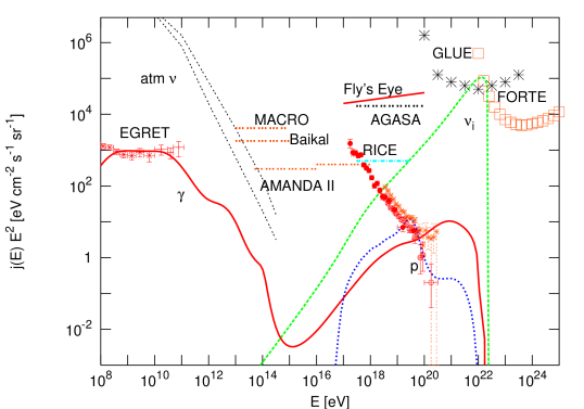
Figure 9: From Ref. ss . Flux predictions for a Z-burst model averaged over flavors and characterized by a neutrino injection flux per comoving volume $\propto E^{-1}$ up to $3\times 10^{22}\,$eV and for redshifts between 0 and 3. The sources are assumed to be exclusive neutrino emitters. All neutrino masses were assumed equal with $m_{\nu}=0.33$ eV and we again assumed maximal mixing between all flavors. The data and upper limits are as in Fig. 2.

However, a combination of new constraints discussed in the previous sections allows to rule out that the Z-burst mechanism explains a dominant fraction of the observed UHECR flux, even for pure neutrino emitting sources: As discussed in Sect. 8.4, a combination of cosmological data including the WMAP experiment limit the sum of the masses of active neutrinos to $\mathrel{\mathchoice{\lower 3.6pt\vbox{\halign{$\mathsurround=0pt\displaystyle\hfil#\hfil$\cr<\crcr\sim\crcr}}}{\lower 3.6pt\vbox{\halign{$\mathsurround=0pt\textstyle\hfil#\hfil$\cr<\crcr\sim\crcr}}}{\lower 3.6pt\vbox{\halign{$\mathsurround=0pt\scriptstyle\hfil#\hfil$\cr<\crcr\sim\crcr}}}{\lower 3.6pt\vbox{\halign{$\mathsurround=0pt\scriptscriptstyle\hfil#\hfil$\cr<\crcr\sim\crcr}}}}1\,$eV hannestad . In Sects. 8.1, 8.2 we have seen that solar and atmospheric neutrino oscillations indicate that individual neutrino masses are nearly degenerate on this scale maltoni , and thus the neutrino mass per flavor must satisfy $m_{\nu}\mathrel{\mathchoice{\lower 3.6pt\vbox{\halign{$\mathsurround=0pt\displaystyle\hfil#\hfil$\cr<\crcr\sim\crcr}}}{\lower 3.6pt\vbox{\halign{$\mathsurround=0pt\textstyle\hfil#\hfil$\cr<\crcr\sim\crcr}}}{\lower 3.6pt\vbox{\halign{$\mathsurround=0pt\scriptstyle\hfil#\hfil$\cr<\crcr\sim\crcr}}}{\lower 3.6pt\vbox{\halign{$\mathsurround=0pt\scriptscriptstyle\hfil#\hfil$\cr<\crcr\sim\crcr}}}}0.33\,$eV. However, for such masses phase space constraints limit the possible over-density of neutrinos in our Local Group of galaxies to $\mathrel{\mathchoice{\lower 3.6pt\vbox{\halign{$\mathsurround=0pt\displaystyle\hfil#\hfil$\cr<\crcr\sim\crcr}}}{\lower 3.6pt\vbox{\halign{$\mathsurround=0pt\textstyle\hfil#\hfil$\cr<\crcr\sim\crcr}}}{\lower 3.6pt\vbox{\halign{$\mathsurround=0pt\scriptstyle\hfil#\hfil$\cr<\crcr\sim\crcr}}}{\lower 3.6pt\vbox{\halign{$\mathsurround=0pt\scriptscriptstyle\hfil#\hfil$\cr<\crcr\sim\crcr}}}}10$ on a length scale of $\sim 1\,$Mpc sm . Since this is considerably smaller than the relevant UHECR loss lengths, neutrino clustering will not significantly reduce the necessary UHE neutrino flux compared to the case of no clustering. For the maximal possible value of the neutrino mass $m_{\nu}\simeq 0.33\,$eV, the neutrino flux required for the Z-burst mechanism to explain the UHECR flux is only in marginal conflict with the FORTE upper limit forte , and factor 2 higher than the new GLUE limit glue , as shown in Fig. 9. For all other cases the conflict with both the GLUE and FORTE limits is considerably more severe. Also note that this argument does not depend on the shape of the low energy tail of the primary neutrino spectrum which could thus be even mono-energetic, as could occur in exclusive tree level decays of superheavy particles into neutrinos gk . However, in addition this possibility has been ruled out by overproduction of GeV $\gamma-$rays due to loop effects in these particle decays bko .

The possibility that the observed UHECR flux is explained by the Z burst scenario involving normal astrophysical sources which produce both neutrinos and photons by pion production is already ruled out by the former EGRET limit: In this case the GeV $\gamma-$ray flux level would have roughly the height of the peak of the neutrino flux multiplied with the squared energy in Fig. 9, thus a factor $\sim 100$ higher than the EGRET level.

Any further reduction in the estimated contribution of the true diffuse extra-galactic $\gamma-$ray background to the observed flux, therefore, leads to more severe constraints on the total EM injection. For example, future $\gamma-$ray detectors such as GLAST glast will test whether the diffuse extragalactic GeV $\gamma-$ray background is truly diffuse or partly consists of discrete sources that could not be resolved by EGRET. Astrophysical discrete contributions such as from intergalactic shocks are in fact expected astrocontr . This could further improve the cascade limit to the point where even acceleration scenarios may become seriously constrained.

9.3 New Primary Particles

A possible way around the problem of missing counterparts within acceleration scenarios is to propose primary particles whose range is not limited by interactions with the CMB. Within the Standard Model the only candidate is the neutrino, whereas in extensions of the Standard Model one could think of new neutrals such as axions or stable supersymmetric elementary particles. Such options are mostly ruled out by the tension between the necessity of a small EM coupling to avoid the GZK cutoff and a large hadronic coupling to ensure normal air showers ggs . Also suggested have been new neutral hadronic bound states of light gluinos with quarks and gluons, so-called R-hadrons that are heavier than nucleons, and therefore have a higher GZK threshold cfk , as can be seen from Eq. (78). Since this too seems to be disfavored by accelerator constraints gluino we will here focus on neutrinos.

In both the neutrino and new neutral stable particle scenario the particle propagating over extragalactic distances would have to be produced as a secondary in interactions of a primary proton that is accelerated in a powerful active galactic nucleus which can, in contrast to the case of EAS induced by nucleons, nuclei, or $\gamma-$rays, be located at high redshift. Consequently, these scenarios predict a correlation between primary arrival directions and high redshift sources. In fact, possible evidence for a correlation of UHECR arrival directions with compact radio quasars and BL-Lac objects, some of them possibly too far away to be consistent with the GZK effect, was recently reported bllac . The main challenge in these correlation studies is the choice of physically meaningful source selection criteria and the avoidance of a posteriori statistical effects. However, a moderate increase in the observed number of events will most likely confirm or rule out the correlation hypothesis. Note, however, that these scenarios require the primary proton to be accelerated up to at least $10^{21}\,$eV, demanding a very powerful astrophysical accelerator.

9.4 New Neutrino Interactions

Neutrino primaries have the advantage of being well established particles. However, within the Standard Model their interaction cross section with nucleons shown in Fig. 1 falls short by about five orders of magnitude to produce air showers starting high in the atmosphere as observed. Electroweak instantons could change this but this possibility is speculative ew_instanton . The neutrino-nucleon cross section, $\sigma_{\nu N}$, however, can be enhanced by new physics beyond the electroweak scale in the CM frame, or above about a PeV in the nucleon rest frame. Note that the CM energy reached by an UHECR nucleon of energy $E$ interacting with an atmospheric nucleon at rest is $\sqrt{s}\simeq 0.4(E/10^{20}\,{\rm eV})\,$PeV. Neutrino induced air showers may therefore rather directly probe new physics beyond the electroweak scale.

One possibility consists of a large increase in the number of degrees of freedom above the electroweak scale kovesi-domokos . A specific instance of this idea appears in theories with $n$ additional large compact dimensions and a quantum gravity scale $M_{4+n}\sim\,$TeV that has recently received much attention in the literature tev-qg because it provides an alternative solution to the hierarchy problem in grand unifications of gauge interactions without a need of supersymmetry. The idea is to dimensionally reduce the $n+4$ dimensional gravitational action

$$S_{g}=-\frac{M_{4+n}^{2+n}}{16\pi}\int d^{4+n}x\sqrt{-g}R\,,$$ (123)

with $g$ the determinant of the metric and $R$ the Ricci scalar, to four dimensions by integrating out the $n$ compact dimensions. This yields the relation

$$M_{\rm Pl}^{2}=V_{n}M_{4+n}^{2+n}\,,$$ (124)

where $M_{\rm Pl}$ and $V_{n}$ are the four-dimensional Planck mass and the volume of the $n$ extra dimensions, respectively. The weakness of gravity can now be understood as a consequence of the fact that it is the only force that propagates into the extra dimensions: Their large volume dilutes gravitational interactions between the Standard Model particles which are confined to a 3-brane representing our world. For compact extra dimensions, gravity would only be modified at scales below

$$r_{n}\simeq M^{-1}_{4+n}\left(\frac{M_{\rm Pl}}{M_{4+n}}\right)^{2/n}\simeq 2\times 10^{-17}\left(\frac{{\rm TeV}}{M_{4+n}}\right)\left(\frac{M_{\rm Pl}}{M_{4+n}}\right)^{2/n}\,{\rm cm}\,,$$ (125)

which is $r_{n}\mathrel{\mathchoice{\lower 3.6pt\vbox{\halign{$\mathsurround=0pt\displaystyle\hfil#\hfil$\cr<\crcr\sim\crcr}}}{\lower 3.6pt\vbox{\halign{$\mathsurround=0pt\textstyle\hfil#\hfil$\cr<\crcr\sim\crcr}}}{\lower 3.6pt\vbox{\halign{$\mathsurround=0pt\scriptstyle\hfil#\hfil$\cr<\crcr\sim\crcr}}}{\lower 3.6pt\vbox{\halign{$\mathsurround=0pt\scriptscriptstyle\hfil#\hfil$\cr<\crcr\sim\crcr}}}}1\,$mm for $n\geq 2$, $M_{4+n}\mathrel{\mathchoice{\lower 3.6pt\vbox{\halign{$\mathsurround=0pt\displaystyle\hfil#\hfil$\cr>\crcr\sim\crcr}}}{\lower 3.6pt\vbox{\halign{$\mathsurround=0pt\textstyle\hfil#\hfil$\cr>\crcr\sim\crcr}}}{\lower 3.6pt\vbox{\halign{$\mathsurround=0pt\scriptstyle\hfil#\hfil$\cr>\crcr\sim\crcr}}}{\lower 3.6pt\vbox{\halign{$\mathsurround=0pt\scriptscriptstyle\hfil#\hfil$\cr>\crcr\sim\crcr}}}}\,$TeV, and thus consistent with gravity tests at small distances. In contrast, non-gravitational interactions are confined to the 3-brane and thus the Standard Model is not modified.

The neutrino-nucleon cross section in these frameworks is obtained by substituting the new fundamental cross section $\sigma_{i}(xs,Q)$ for the electroweak cross section at the parton level in Eq. (75),

$$\frac{d\sigma^{\nu X}}{dxdy}=\sum_{i}f_{i}(x,Q)\sigma_{i}(xs,Q)\,.$$ (126)

One of the largest contributions to the neutrino-nucleon cross section turns out to be the production on our 3-brane of microscopic black holes which are solutions of $4+n$-dimensional gravity described by Eq. (123). These cross sections scale as $(s/M_{4+n}^{2})^{1/(n+1)}$ for $s\mathrel{\mathchoice{\lower 3.6pt\vbox{\halign{$\mathsurround=0pt\displaystyle\hfil#\hfil$\cr>\crcr\sim\crcr}}}{\lower 3.6pt\vbox{\halign{$\mathsurround=0pt\textstyle\hfil#\hfil$\cr>\crcr\sim\crcr}}}{\lower 3.6pt\vbox{\halign{$\mathsurround=0pt\scriptstyle\hfil#\hfil$\cr>\crcr\sim\crcr}}}{\lower 3.6pt\vbox{\halign{$\mathsurround=0pt\scriptscriptstyle\hfil#\hfil$\cr>\crcr\sim\crcr}}}}M_{4+n}^{2}$. Their UV-divergence is due to the non-renormalizable, classical character of the gravitational interaction Eq. (123) in the sense of Sect. 3. The production of compact branes, completely wrapped around the extra dimensions, may provide even larger contributions aco . The resulting total cross sections can be larger than in the Standard Model by up to a factor $\sim 100$ if $M_{4+n}\sim\,$TeV fs . However, extra dimensions with a flat geometry are severely constrained by astrophysics: Core collapse of massive stars would lead to production of gravitational excitations in the large compact extra dimensions, mostly by nucleon-nucleon bremsstrahlung. These so called Kaluza-Klein gravitons of mass $m_{g}$ are then gravitationally trapped around the newly born neutron star during their livetime $\tau\sim M_{\rm Pl}^{2}/m_{g}^{3}\sim 10^{13}(10\,{\rm MeV}/m_{g})^{3}\,$yr. Their subsequent decay into two $\gamma-$rays would make neutron stars shine in $\gamma-$rays. The non-observation of such emission leads to lower bounds on $M_{4+n}$ which decrease with increasing $n$, starting with $M_{5}\mathrel{\mathchoice{\lower 3.6pt\vbox{\halign{$\mathsurround=0pt\displaystyle\hfil#\hfil$\cr>\crcr\sim\crcr}}}{\lower 3.6pt\vbox{\halign{$\mathsurround=0pt\textstyle\hfil#\hfil$\cr>\crcr\sim\crcr}}}{\lower 3.6pt\vbox{\halign{$\mathsurround=0pt\scriptstyle\hfil#\hfil$\cr>\crcr\sim\crcr}}}{\lower 3.6pt\vbox{\halign{$\mathsurround=0pt\scriptscriptstyle\hfil#\hfil$\cr>\crcr\sim\crcr}}}}10^{5}\,$TeV and going down to $M_{9}\mathrel{\mathchoice{\lower 3.6pt\vbox{\halign{$\mathsurround=0pt\displaystyle\hfil#\hfil$\cr>\crcr\sim\crcr}}}{\lower 3.6pt\vbox{\halign{$\mathsurround=0pt\textstyle\hfil#\hfil$\cr>\crcr\sim\crcr}}}{\lower 3.6pt\vbox{\halign{$\mathsurround=0pt\scriptstyle\hfil#\hfil$\cr>\crcr\sim\crcr}}}{\lower 3.6pt\vbox{\halign{$\mathsurround=0pt\scriptscriptstyle\hfil#\hfil$\cr>\crcr\sim\crcr}}}}1\,$TeV and still lower values for larger $n$ hannestad1 ; casse , for flat compact extra dimensions. This implies that significant contributions to the neutrino-nucleon cross section in these extra dimension scenarios require either $n\geq 5$ extra dimensions or a warped geometry.

Whereas the sub-hadronic scale cross sections obtained in some extra dimension scenarios are still too small to be consistent with observed air showers and thus to explain the observed UHECR events kp , they can still have important phenomenological consequences. This is because UHECR data can be used to put constraints on cross sections satisfying $\sigma_{\nu N}(E\mathrel{\mathchoice{\lower 3.6pt\vbox{\halign{$\mathsurround=0pt\displaystyle\hfil#\hfil$\cr>\crcr\sim\crcr}}}{\lower 3.6pt\vbox{\halign{$\mathsurround=0pt\textstyle\hfil#\hfil$\cr>\crcr\sim\crcr}}}{\lower 3.6pt\vbox{\halign{$\mathsurround=0pt\scriptstyle\hfil#\hfil$\cr>\crcr\sim\crcr}}}{\lower 3.6pt\vbox{\halign{$\mathsurround=0pt\scriptscriptstyle\hfil#\hfil$\cr>\crcr\sim\crcr}}}}10^{19}\,{\rm eV})\mathrel{\mathchoice{\lower 3.6pt\vbox{\halign{$\mathsurround=0pt\displaystyle\hfil#\hfil$\cr<\crcr\sim\crcr}}}{\lower 3.6pt\vbox{\halign{$\mathsurround=0pt\textstyle\hfil#\hfil$\cr<\crcr\sim\crcr}}}{\lower 3.6pt\vbox{\halign{$\mathsurround=0pt\scriptstyle\hfil#\hfil$\cr<\crcr\sim\crcr}}}{\lower 3.6pt\vbox{\halign{$\mathsurround=0pt\scriptscriptstyle\hfil#\hfil$\cr<\crcr\sim\crcr}}}}10^{-27}\,{\rm cm}^{2}$. Particles with such cross sections would give rise to horizontal air showers which have not yet been observed. Resulting upper limits on their fluxes assuming the Standard Model cross section Eq. (7) are shown in Fig. 2. Comparison with the “cosmogenic” neutrino flux produced by UHECRs interacting with the CMB then results in upper limits on the cross section which are about a factor 1000 larger than Eq. (7) in the energy range between $\simeq 10^{17}\,$eV and $\simeq 10^{19}\,$eV mr ; tol ; afgs . The projected sensitivity of future experiments shown in Fig. 3 indicate that these limits could be lowered down to the Standard Model cross section afgs . In case of a detection of penetrating events the degeneracy of the cross section with the unknown neutrino flux could be broken by comparing the rates of horizontal air showers with the ones of Earth skimming events kw . This would allow to “measure” the neutrino-nucleon cross section at energies unreachable by any forseeable terrestrial accelerator !

9.5 Violation of Lorentz Invariance

The most elegant solution to the problem of apparently missing nearby sources of UHECRs and for their putative correlation with high redshift sources would be to speculate that the GZK effect does not exist theoretically. A number of authors pointed out vli_others ; cg that this may be possible by allowing violation of Lorentz invariance (VLI) by a tiny amount that is consistent with all current experiments. At a purely theoretical level, several quantum gravity models including some based on string theories do in fact predict non-trivial modifications of space-time symmetries that also imply VLI at extremely short distances (or equivalently at extremely high energies); see e.g., Ref. amelino-piran and references therein. These theories are, however, not yet in forms definite enough to allow precise quantitative predictions of the exact form of the possible VLI. Current formulations of the effects of a possible VLI on high energy particle interactions relevant in the context of UHECR, therefore, adopt a phenomenological approach in which the form of the possible VLI is parametrized in various ways. VLI generally implies the existence of a universal preferred frame which is usually identified with the frame that is comoving with the expansion of the Universe, in which the CMB is isotropic.

A direct way of introducing VLI is through a modification of the standard dispersion relation, $E^{2}-p^{2}=m^{2}$, between energy $E$ and momentum $p=|\vec{p}|$ of particles, $m$ being the invariant mass of the particle. Currently there is no unique way of parameterizing the possible modification of this relation in a Lorentz non-invariant theory. We discuss here a parameterization of the modified dispersion relation which covers most of the qualitative cases discussed in the literature and, for certain parameter values, allows to completely evade the GZK limit,

$$E^{2}-p^{2}-m^{2}\simeq-2dE^{2}-\xi\frac{E^{3}}{M_{\rm Pl}}-\zeta\frac{E^{4}}{M^{2}_{\rm Pl}}\,.$$ (127)

Here, the Planck mass $M_{\rm Pl}$ characterizes non-renormalizable effects with dimensionless coefficients $\xi$ and $\zeta$, and the dimensionless constant $d$ exemplifies VLI effects due to renormalizable terms in the Lagrangian, see the discussion in Sect. 3. The standard Lorentz invariant dispersion relation is recovered in the limit $\xi,\zeta,d\to 0$.

The constants $d\neq 0$ can break Lorentz invariance spontaneously when certain Lorentz tensors $c_{\mu\nu}$ have couplings to fermions of the form $d_{\mu\nu}\bar{\psi}\gamma^{\mu}\partial^{\nu}\psi$, and acquire vacuum expectation values of the form $\langle d_{\mu\nu}\rangle=d\delta_{\mu}^{0}\delta_{\nu}^{0}$. If rotational invariance and gauge symmetry are preserved, such renormalizable Lorentz invariance breaking terms in the Lagrangian, whose Lorentz invariant part is given by Eq. (58), are characterized by a single time-like vector $u^{\mu}$, with $u^{\mu}u_{\mu}=-1$, which defines a preferred reference frame ck . The dimensionless terms can be interpreted as a change of the maximal particle velocity cg $v_{\rm max}=\partial E/\partial p|_{E,p\gg m}\simeq 1-d$. At a fixed energy $E$ one has the correspondence $d\to(\xi/2)(E/M_{\rm Pl})+(\zeta/2)(E/M_{\rm Pl})^{2}$, as can be seen from Eq. (127).

Within effective field theory, effects of first order in $M^{-1}_{\rm Pl}$, $\xi\neq 0$, arise from the most general terms of the form

$$\frac{\kappa}{2M_{\rm Pl}}u^{\mu}F_{\mu\nu}(u\cdot\partial)u_{\lambda}\tilde{F}^{\lambda\nu}+\frac{1}{2M_{\rm Pl}}u^{\mu}\bar{\psi}\gamma_{\mu}(\lambda_{1}+\lambda_{2}\gamma_{5})(u\cdot\partial)^{2}\psi\,,$$ (128)

where $\tilde{F}$ denotes the dual of the field strength $F$. For photons and electrons this leads to $\xi=\pm\kappa$ and $\xi=\lambda_{1}\pm\lambda_{2}$, respectively, in Eq. (127), where $\pm$ refers to helicity which remains conserved in the presence of the terms Eq. (128) pospelov . These terms also violate $CPT$. Effects of first order in $M^{-1}_{\rm Pl}$, $\xi\neq 0$, are possible, for example, in non-critical Liouville string theory due to recoiling D-branes emn . Finally, in critical string theory, effects second order in $M^{-1}_{\rm Pl}$, $\zeta\neq 0$, can be induced due to quantum gravity effects.

Interestingly, it has been pointed out recently that in the supersymmetric Standard Model VLI terms must be non-renormalizable and do not lead to modifications of any dispersion relations nibbelink .

Now, consider the GZK photo-pion production process in which a nucleon of energy $E$, momentum $p$ and mass $m_{N}$ collides head-on with a CMB photon of energy $\epsilon$ producing a pion and a recoiling nucleon. The threshold initial momentum of the nucleon for this process according to standard Lorentz invariant kinematics is

$$p_{{\rm th},0}=(m_{\pi}^{2}+2m_{\pi}m_{N})/4\epsilon\,,$$ (129)

where $m_{\pi}$ and $m_{N}$ are the pion and nucleon masses, respectively. Assuming exact energy-momentum conservation but using the modified dispersion relation given above, in the ultra-relativistic regime $m\ll p\ll M$, and neglecting sub-leading terms, the new nucleon threshold momentum $p_{\rm th}$ under the modified dispersion relation Eq. (127) for $d=0$ satisfies aloisio

$$-\beta x^{4}-\alpha x^{3}+x-1=0\,,$$ (130)

where $x=p_{\rm th}/p_{{\rm th},0}$, and

$$\alpha = \frac{2\xi p_{{\rm th},0}^{3}}{(m_{\pi}^{2}+2m_{\pi}m_{N})M_{\rm Pl}}\frac{m_{\pi}m_{N}}{(m_{\pi}+m_{N})^{2}}\,,$$ (131)

$$\beta = \frac{3\zeta p_{{\rm th},0}^{4}}{2(m_{\pi}^{2}+2m_{\pi}m_{N})M^{2}_{\rm Pl}}\frac{m_{\pi}m_{N}}{(m_{\pi}+m_{N})^{2}}\,.$$

One can show that the same modified dispersion relation Eq. (127) leads to the same condition Eq. (130) for absorption of high energy gamma rays through $e^{+}e^{-}$ pair production on the infrared, microwave or radio backgrounds, if one substitutes $p_{{\rm th},0}=m^{2}_{e}/\epsilon$, $\alpha=\xi p_{{\rm th},0}^{3}/(8m^{2}_{e}M_{\rm Pl})$, $\beta=3\zeta p_{{\rm th},0}^{4}/(16m^{2}_{e}M^{2}_{\rm Pl})$, where $m_{e}$ is the electron mass.

If $\xi,\zeta\simeq 1$, there is no real positive solution of Eq. (130), implying that the GZK process does not take place and consequently the GZK cutoff effect disappears completely. Thus UHE nucleons and/or photons will be able to reach Earth from any distance. On the other hand, if future UHECR data confirm the presence of a GZK cutoff at some energy then that would imply upper limits on the couplings $\xi$ and $\zeta$, thus probing specific Lorentz non-invariant theories. If $p_{\rm th}\simeq p_{{\rm th},0}$, one could conclude from Eq. (130) that $\alpha,\beta\mathrel{\mathchoice{\lower 3.6pt\vbox{\halign{$\mathsurround=0pt\displaystyle\hfil#\hfil$\cr<\crcr\sim\crcr}}}{\lower 3.6pt\vbox{\halign{$\mathsurround=0pt\textstyle\hfil#\hfil$\cr<\crcr\sim\crcr}}}{\lower 3.6pt\vbox{\halign{$\mathsurround=0pt\scriptstyle\hfil#\hfil$\cr<\crcr\sim\crcr}}}{\lower 3.6pt\vbox{\halign{$\mathsurround=0pt\scriptscriptstyle\hfil#\hfil$\cr<\crcr\sim\crcr}}}}1$, which translates into $|\xi|\mathrel{\mathchoice{\lower 3.6pt\vbox{\halign{$\mathsurround=0pt\displaystyle\hfil#\hfil$\cr<\crcr\sim\crcr}}}{\lower 3.6pt\vbox{\halign{$\mathsurround=0pt\textstyle\hfil#\hfil$\cr<\crcr\sim\crcr}}}{\lower 3.6pt\vbox{\halign{$\mathsurround=0pt\scriptstyle\hfil#\hfil$\cr<\crcr\sim\crcr}}}{\lower 3.6pt\vbox{\halign{$\mathsurround=0pt\scriptscriptstyle\hfil#\hfil$\cr<\crcr\sim\crcr}}}}10^{-13}$ for the first order effects, and $|\zeta|\mathrel{\mathchoice{\lower 3.6pt\vbox{\halign{$\mathsurround=0pt\displaystyle\hfil#\hfil$\cr<\crcr\sim\crcr}}}{\lower 3.6pt\vbox{\halign{$\mathsurround=0pt\textstyle\hfil#\hfil$\cr<\crcr\sim\crcr}}}{\lower 3.6pt\vbox{\halign{$\mathsurround=0pt\scriptstyle\hfil#\hfil$\cr<\crcr\sim\crcr}}}{\lower 3.6pt\vbox{\halign{$\mathsurround=0pt\scriptscriptstyle\hfil#\hfil$\cr<\crcr\sim\crcr}}}}10^{-6}$ for the second order effects, $\xi=0$ aloisio . These values correspond to values $|d|\mathrel{\mathchoice{\lower 3.6pt\vbox{\halign{$\mathsurround=0pt\displaystyle\hfil#\hfil$\cr<\crcr\sim\crcr}}}{\lower 3.6pt\vbox{\halign{$\mathsurround=0pt\textstyle\hfil#\hfil$\cr<\crcr\sim\crcr}}}{\lower 3.6pt\vbox{\halign{$\mathsurround=0pt\scriptstyle\hfil#\hfil$\cr<\crcr\sim\crcr}}}{\lower 3.6pt\vbox{\halign{$\mathsurround=0pt\scriptscriptstyle\hfil#\hfil$\cr<\crcr\sim\crcr}}}}10^{-23}$ for the paremeters of renormalizable VLI. Confirmation of a cut-off for TeV photons with next-generation $\gamma-$ray observatories would lead to somewhat weaker constraints tev .

More generally, modification of reaction kinematics or new reaction channels are expected whenever the terms on the right hand side of Eq. (127) become comparable to $m^{2}$, in rough numbers,

$$d \mathrel{\mathchoice{\lower 3.6pt\vbox{\halign{$\mathsurround=0pt\displaystyle\hfil#\hfil$\cr>\crcr\sim\crcr}}}{\lower 3.6pt\vbox{\halign{$\mathsurround=0pt\textstyle\hfil#\hfil$\cr>\crcr\sim\crcr}}}{\lower 3.6pt\vbox{\halign{$\mathsurround=0pt\scriptstyle\hfil#\hfil$\cr>\crcr\sim\crcr}}}{\lower 3.6pt\vbox{\halign{$\mathsurround=0pt\scriptscriptstyle\hfil#\hfil$\cr>\crcr\sim\crcr}}}} \frac{m^{2}}{2E^{2}}\simeq 5\times 10^{-23}\left(\frac{m}{{\rm GeV}}\right)^{2}\left(\frac{E}{10^{20}{\rm eV}}\right)^{-2}\,,$$ (140)

$$\xi \mathrel{\mathchoice{\lower 3.6pt\vbox{\halign{$\mathsurround=0pt\displaystyle\hfil#\hfil$\cr>\crcr\sim\crcr}}}{\lower 3.6pt\vbox{\halign{$\mathsurround=0pt\textstyle\hfil#\hfil$\cr>\crcr\sim\crcr}}}{\lower 3.6pt\vbox{\halign{$\mathsurround=0pt\scriptstyle\hfil#\hfil$\cr>\crcr\sim\crcr}}}{\lower 3.6pt\vbox{\halign{$\mathsurround=0pt\scriptscriptstyle\hfil#\hfil$\cr>\crcr\sim\crcr}}}} \frac{M_{\rm Pl}m^{2}}{E^{3}}\simeq 10^{-14}\left(\frac{m}{{\rm GeV}}\right)^{2}\left(\frac{E}{10^{20}{\rm eV}}\right)^{-3}\,,$$ (149)

$$\zeta \mathrel{\mathchoice{\lower 3.6pt\vbox{\halign{$\mathsurround=0pt\displaystyle\hfil#\hfil$\cr>\crcr\sim\crcr}}}{\lower 3.6pt\vbox{\halign{$\mathsurround=0pt\textstyle\hfil#\hfil$\cr>\crcr\sim\crcr}}}{\lower 3.6pt\vbox{\halign{$\mathsurround=0pt\scriptstyle\hfil#\hfil$\cr>\crcr\sim\crcr}}}{\lower 3.6pt\vbox{\halign{$\mathsurround=0pt\scriptscriptstyle\hfil#\hfil$\cr>\crcr\sim\crcr}}}} \frac{M_{\rm Pl}^{2}m^{2}}{E^{4}}\simeq 10^{-6}\left(\frac{m}{{\rm GeV}}\right)^{2}\left(\frac{E}{10^{20}{\rm eV}}\right)^{-4}\,.$$ (158)

Note that by far the smallest parameter values would be probed by particles with the smallest mass, specifically the neutrino, $m\mathrel{\mathchoice{\lower 3.6pt\vbox{\halign{$\mathsurround=0pt\displaystyle\hfil#\hfil$\cr<\crcr\sim\crcr}}}{\lower 3.6pt\vbox{\halign{$\mathsurround=0pt\textstyle\hfil#\hfil$\cr<\crcr\sim\crcr}}}{\lower 3.6pt\vbox{\halign{$\mathsurround=0pt\scriptstyle\hfil#\hfil$\cr<\crcr\sim\crcr}}}{\lower 3.6pt\vbox{\halign{$\mathsurround=0pt\scriptscriptstyle\hfil#\hfil$\cr<\crcr\sim\crcr}}}}\,$eV at the highest energies. This makes the prospects of future detections of cosmogenic neutrinos, see, e.g., Fig. 2, very exciting also for VLI constraints.

In addition, the non-renormalizable terms in the dispersion relation Eq. (127) imply a change in the group velocity which for the first-order term leads to time delays over distances $r$ given by

$$\Delta t\simeq\xi r\frac{E}{M_{\rm Pl}}\simeq\xi\left(\frac{r}{100\,{\rm Mpc}}\right)\left(\frac{E}{{\rm TeV}}\right)\,{\rm sec}\,.$$ (159)

For $|\xi|\sim 1$ such time delays could be measurable, for example, by fitting the arrival times of $\gamma-$rays arriving from $\gamma-$ray bursts to the predicted energy dependence.

We mention that if VLI is due to modification of the space-time structure expected in some theories of quantum gravity, for example, then the strict energy-momentum conservation assumed in the above discussion, which requires space-time translation invariance, is not guaranteed in general, and then the calculation of the modified particle interaction thresholds becomes highly non-trivial and non-obvious. Also, it is possible that a Lorentz non-invariant theory while giving a modified dispersion relation also imposes additional kinematic structures such as a modified law of addition of momenta. Indeed, Ref. amelino-piran gives an example of a so-called $\kappa$-Minkowski non-commutative space-time in which the modified dispersion relation has the same form as in Eq. (127) but there is also a modified momentum addition rule which compensates for the effect of the modified dispersion relation on the particle interaction thresholds discussed above leaving the threshold momentum unaffected and consequently the GZK problem unsolved. In scenarios where the relativity of inertial frames is preserved by a non-linear representation of the Poincaré group, thresholds are in general significantly modified only if the effective mass scale $M_{\rm Pl}/\xi$ is of the order of the unmodified threshold energy in the laboratory frame ms .

There are several other fascinating effects of allowing a small VLI, some of which are relevant for the question of origin and propagation of UHECR. For example, any movement relative to the preferred frame defined by $u^{\mu}$ in Eq. (128) gives rise to spatial anisotropy. Clock comparison and spin precession experiments then lead to limits on the dimensionless parameters in Eq. (128) between ${\cal O}(1)$ and ${\cal O}(10^{-8})$, depending on the particle pospelov . Similar limits result from astrophysical arguments: The observation of polarized MeV synchrotron radiation from electrons in the Crab nebula implies the absence of vacuum Čerenkov radiation $e\to e\gamma$ for electrons up to energies $E\sim 1.5\,$PeV jlms ; jlm . This process can become possible if the electron speed becomes larger than the speed of light at high energies and leads to limits on VLI of size comparable to the before mentioned laboratory constraints jlms ; jlm . These constraints basically rule out effects of order $E/M_{\rm Pl}$ which might be a challenge for certain quantum gravity scenarios pr . Note that these current constraints on VLI parameters still allow strong modification of GZK kinematics by VLI parameters of the order given in Eq. (149).

9.6 Cosmic Magnetic Fields and Their Influence on Ultra-High Energy Cosmic Ray Propagation

Cosmic magnetic fields are inextricably linked with cosmic rays in several respects. First, they play a central role in Fermi shock acceleration. Second, large scale extra-galactic magnetic fields (EGMF) can cause significant deflection of charged cosmic rays during propagation and thus obviously complicate the relation between observed UHECR distributions and their sources.

Magnetic fields are omnipresent in the Universe, but their true origin is still unclear bt_review . Magnetic fields in galaxies are observed with typical strengths of a few micro Gauss, but there are also some indications for fields correlated with larger structures such as galaxy clusters bo_review . Magnetic fields as strong as $\simeq 1\mu G$ in sheets and filaments of the large scale galaxy distribution, such as in our Local Supercluster, are compatible with existing upper limits on Faraday rotation bo_review ; ryu ; blasi . It is also possible that fossil cocoons of former radio galaxies, so called radio ghosts, contribute significantly to the isotropization of UHECR arrival directions mte .

To get an impression of typical deflection angles one can characterize the EGMF by its r.m.s. strength $B$ and a coherence length $l_{c}$. If we neglect energy loss processes for the moment, then the r.m.s. deflection angle over a distance $r\mathrel{\mathchoice{\lower 3.6pt\vbox{\halign{$\mathsurround=0pt\displaystyle\hfil#\hfil$\cr>\crcr\sim\crcr}}}{\lower 3.6pt\vbox{\halign{$\mathsurround=0pt\textstyle\hfil#\hfil$\cr>\crcr\sim\crcr}}}{\lower 3.6pt\vbox{\halign{$\mathsurround=0pt\scriptstyle\hfil#\hfil$\cr>\crcr\sim\crcr}}}{\lower 3.6pt\vbox{\halign{$\mathsurround=0pt\scriptscriptstyle\hfil#\hfil$\cr>\crcr\sim\crcr}}}}l_{c}$ in such a field is $\theta(E,r)\simeq(2rl_{c}/9)^{1/2}/r_{L}$ wm , where the Larmor radius of a particle of charge $Ze$ and energy $E$ is $r_{L}\simeq E/(ZeB)$. In numbers this reads

$$\theta(E,r)\simeq 0.8^{\circ}\,Z\left(\frac{E}{10^{20}\,{\rm eV}}\right)^{-1}\left(\frac{r}{10\,{\rm Mpc}}\right)^{1/2}\left(\frac{l_{c}}{1\,{\rm Mpc}}\right)^{1/2}\left(\frac{B}{10^{-9}\,{\rm G}}\right)\,,$$ (160)

for $r\mathrel{\mathchoice{\lower 3.6pt\vbox{\halign{$\mathsurround=0pt\displaystyle\hfil#\hfil$\cr>\crcr\sim\crcr}}}{\lower 3.6pt\vbox{\halign{$\mathsurround=0pt\textstyle\hfil#\hfil$\cr>\crcr\sim\crcr}}}{\lower 3.6pt\vbox{\halign{$\mathsurround=0pt\scriptstyle\hfil#\hfil$\cr>\crcr\sim\crcr}}}{\lower 3.6pt\vbox{\halign{$\mathsurround=0pt\scriptscriptstyle\hfil#\hfil$\cr>\crcr\sim\crcr}}}}l_{c}$. This expression makes it immediately obvious that fields of fractions of micro Gauss lead to strong deflection even at the highest energies. This goes along with a time delay $\tau(E,r)\simeq r\theta(E,d)^{2}/4\simeq 1.5\times 10^{3}\,Z^{2}(E/10^{20}\,{\rm eV})^{-2}(r/10\,{\rm Mpc})^{2}(l_{c}/{\rm Mpc})(B/10^{-9}\,{\rm G})^{2}\,$yr which can be millions of years. A source visible in UHECRs today could therefore be optically invisible since many models involving, for example, active galaxies as UHECR accelerators, predict variability on shorter time scales.

Quite a few simulations of the effect of extragalactic magnetic fields (EGMF) on UHECRs exist in the literature, but usually idealizing assumptions concerning properties and distributions of sources or EGMF or both are made: In Refs. slb ; ils ; lsb ; sse ; is sources and EGMF follow a pancake profile mimicking the local supergalactic plane. In other studies EGMF have been approximated in a number of fashions: as negligible sommers ; bdm , as stochastic with uniform statistical properties bo ; ynts ; ab , or as organized in spatial cells with a given coherence length and a strength depending as a power law on the local density tanco . Only recently attempts have been made to simulate UHECR propagation in a realistically structured universe sme ; dolag . For now, these simulations are limited to nucleons.

In Ref. sme the magnetized extragalactic environment used for UHECR propagation is produced by a simulation of the large scale structure of the Universe. The simulation was carried out within a computational box of $50\,h^{-1}\,$Mpc length on a side, with normalized Hubble constant $h\equiv H_{0}/(100$ km s^-1 Mpc${}^{-1})$ = 0.67, and using a comoving grid of 512³ zones and 256³ dark matter particles. The EGMF was initialized to zero at simulation start and subsequently its seeds were generated at cosmic shocks through the Biermann battery mechanism kcor97 . Since cosmic shocks form primarily around collapsing structures including filaments, the above approach avoids generating EGMF in cosmic voids.

In Ref. dolag constrained simulations of the local large scale structure were performed and the magnetic smoothed particle hydrodynamics technique was used to follow EGMF evolution. The EGMF was seeded by a uniform seed field of maximal strength compatible with observed rotation measures in galaxy clusters.

The questions considered in these two works were somewhat different, however. In Ref. dolag deflections of UHECR above $4\times 10^{19}\,$eV were computed as a function of the direction to their source which were assumed to be at cosmological distances. This made sense, because (i) the constrained simulations gives a viable model of our local cosmic neighborhood within about 100 Mpc, at least on scales beyond a few Mpc and (ii) the deflections typically were found to be smaller than a few degrees. Concrete source distributions were not considered.

Figure 10: Log-scale two-dimensional cut through magnetic field total strength in Gauss (color scale in Gauss) for a scenario in good agreement with UHECR data studied in Ref. sme . The observer is in the center of the figures and is marked by a star. The EGMF strength at the observer is $\simeq 10^{-11}\,$G.

In contrast, Ref. sme was not concerned with concrete sky distributions or deflection maps because the simulation was unconstrained and thus only gave a typical large scale structure model and not our concrete local neighborhood. Instead, the question was asked which observer positions and source distributions and characteristics lead to UHECR distributions whose spherical multi-poles for $l\leq 10$ and auto-correlation at angles $\theta\mathrel{\mathchoice{\lower 3.6pt\vbox{\halign{$\mathsurround=0pt\displaystyle\hfil#\hfil$\cr<\crcr\sim\crcr}}}{\lower 3.6pt\vbox{\halign{$\mathsurround=0pt\textstyle\hfil#\hfil$\cr<\crcr\sim\crcr}}}{\lower 3.6pt\vbox{\halign{$\mathsurround=0pt\scriptstyle\hfil#\hfil$\cr<\crcr\sim\crcr}}}{\lower 3.6pt\vbox{\halign{$\mathsurround=0pt\scriptscriptstyle\hfil#\hfil$\cr<\crcr\sim\crcr}}}}20^{\circ}$ are consistent with observations. As a result it was found that (i) the observed large scale UHECR isotropy requires the neighborhood within a few Mpc of the observer is characterized by weak magnetic fields below $0.1\,\mu$G, and (ii) once that choice is made, current data do not strongly discriminate between uniform and structured source distributions and between negligible and considerable deflection. Nevertheless, current data moderately favor a scenario in which (iii) UHECR sources have a density $n_{s}\sim 10^{-5}\,{\rm Mpc}^{-3}$ and follow the matter distribution and (iv) magnetic fields are relatively pervasive within the large scale structure, including filaments, and with a strength of order of a $\mu$G in galaxy clusters. A two-dimensional cut through the EGMF environment of the observer in a typical such scenario is shown in Fig. 10.

It was also studied in Ref. sme how future data of considerably increased statistics can be used to learn more about EGMF and source characteristics. In particular, low auto-correlations at degree scales imply magnetized sources quite independent of other source characteristics such as their density. The latter can only be estimated from the auto-correlations halfway reliably if magnetic fields have negligible impact on propagation. This is because if sources are immersed in considerable magnetic fields, their images are smeared out, which also smears out the auto-correlation function over several degrees. For a sufficiently high source density, individual images can thus overlap and sensitivity to source density is consequently lost. The statistics expected from next generation experiments such as Pierre Auger auger and EUSO euso should be sufficient to test source magnetization by the auto-correlation function sme .

Figure 11: The cumulative distribution of UHECR deflection angles $\alpha$ with respect to the line of sight to the sources. This is for a scenario from Ref. sme in good agreement with UHECR data, where the sources follow the baryon density and have average density $n_{s}=2.4\times 10^{-5}\,{\rm Mpc}^{-3}$, and the EGMF included in the large scale structure simulation reaches several micro Gauss in the most prominent galaxy cluster. Shown are the average (middle, histogram) and 1-$\sigma$ variations (upper and lower curves) above $4\times 10^{19}\,$eV, over 24 realizations varying in the positions and luminosities $Q_{i}$ of individual sources, the latter assumed to be distributed as $dn_{s}/dQ_{i}\propto Q_{i}^{-2.2}$ with $1\leq Q_{i}\leq 100$ in arbitrary units. Also given on top of the figure are average and variances of the distributions.

Interestingly, however, there is a considerable quantifiable difference in the typical deflection angles predicted by the two EGMF scenarios in Refs. sme ; dolag that can not be compensated by specific source distributions: Even for homogeneous source distributions, the average deflection angle for UHECRs above $4\times 10^{19}\,$eV obtained in Ref. sme is much larger than in Ref. dolag , as can be seen in Fig. 11. In fact, even if the magnetic field strength is reduced by a factor 10 in the simulations of Ref. sme , the average deflection angle above $4\times 10^{19}\,$eV is still $\sim 30^{\circ}$, only a factor $\simeq 2.2$ smaller. This non-linear behavior of deflection with field normalization is mostly due to the strongly non-homogeneous character of the EGMF.

Figure 12: The cumulative filling factors for EGMF strength in the simulations used in Ref. sme above (decreasing curve) and below (increasing curve) a given threshold, as a function of that threshold.

Most of these differences are probably due to the different numerical models for the magnetic fields. Although Ref. dolag start with uniform seed fields, whereas in Ref. sme seed fields are injected at shocks, by itself, this difference should not influence the resulting EGMF very much at late times, at least inside galaxy clusters ryu . It should be noted, however, that in the filaments, where the gas motions are more uniform, the simulated magnetic fields may depend to a certain extent on the initial seed fields although that is not trivial to quantify in general terms. In addition, numerical resolution may play an important role because it affects the amplification and the topological structure of the magnetic fields, both of which are important for the normalization procedure, see below. The resolution in Ref. sme is constant and much better in filaments and voids but worse in the core of galaxy clusters than the (variable) resolution in Ref. dolag . If in both simulations the magnetic fields are normalized to (or reproduce) the same “observed” values in the core of rich clusters then obviously their values in the filaments will be very different for the reasons outlined above. This may partly explain why the contribution of filaments to UHECR deflection is more important in Ref. sme , although a more detailed analysis and comparison are required to settle the issue. In any case, the magnetic fields obtained in Ref. sme seem to be quite extended, as can be seen in Fig. 12: About 10% of the volume is filled with fields stronger than 10 nano Gauss, and a fraction of $10^{-3}$ is filled by fields above a micro Gauss. Furthermore, typical deflection angles change at most by a factor of 2 if magnetic field normalization is decreased by a factor 10 or seed fields are chosen as uniform in these simulations. The different amounts of deflection obtained in the simulations of Refs. sme ; dolag show that the distribution of EGMF and their effects on UHECR propagation are currently rather uncertain.

Finally we note that these studies should be extended to include heavy nuclei prepa since there are indications that a fraction as large as 80% of iron nuclei may exist above $10^{19}\,$eV watson . As a consequence, even in the EGMF scenario of Ref. dolag deflections could be considerable and may not allow particle astronomy along many lines of sight: The distribution of deflection angles in Ref. dolag shows that deflections of protons above $4\times 10^{19}\,$eV of $\mathrel{\mathchoice{\lower 3.6pt\vbox{\halign{$\mathsurround=0pt\displaystyle\hfil#\hfil$\cr>\crcr\sim\crcr}}}{\lower 3.6pt\vbox{\halign{$\mathsurround=0pt\textstyle\hfil#\hfil$\cr>\crcr\sim\crcr}}}{\lower 3.6pt\vbox{\halign{$\mathsurround=0pt\scriptstyle\hfil#\hfil$\cr>\crcr\sim\crcr}}}{\lower 3.6pt\vbox{\halign{$\mathsurround=0pt\scriptscriptstyle\hfil#\hfil$\cr>\crcr\sim\crcr}}}}1^{\circ}$ cover a considerable fraction of the sky. Suppression of deflection along typical lines of sight by small filling factors of deflectors is thus unimportant in this case. The deflection angle of any nucleus at a given energy passing through such areas will therefore be roughly proportional to its charge as long as energy loss lengths are larger than a few tens of Mpc bils . Deflection angles of $\sim 20^{\circ}$ at $\sim 4\times 10^{19}\,$eV should thus be the rule for iron nuclei. In contrast to the contribution of our Galaxy to deflection which can be of comparable size but may be corrected for within sufficiently detailed models of the galactic field, the extra-galactic contribution would be stochastic. Statistical methods are therefore likely to be necessary to learn about UHECR source distributions and characteristics. In addition, should a substantial heavy composition be experimentally confirmed up to the highest energies, some sources would have to be surprisingly nearby, within a few Mpc, otherwise only low mass spallation products would survive propagation er .

The putative clustered component of the UHECR flux whose fraction of the total flux seems to increase with energy teshima1 may play a key role in this context. It could be caused by discrete sources in directions with small deflection. Spectrum and composition of the flux from such sources could still by modified considerably by magnetic fields concentrated around the source sse ; sigl . For example, since, apart from energy losses, cosmic rays of same rigidity $Z/A$ are deflected similarly by cosmic magnetic fields, one may expect that the composition of the clustered component may become heavier with increasing energy. Indeed, in Ref. teshima it was speculated that the AGASA clusters may be consistent with consecutive He, Be-Mg, and Fe bumps.

It thus seems evident that the influence of large scale cosmic magnetic fields on ultra-high energy cosmic ray propagation is currently hard to quantify and may not allow to do “particle astronomy” along most lines of sight, especially if a significant heavy nucleus component is present above $10^{19}\,$eV.

References

- (1) D. H. Perkins (1987). Introduction to High Energy Physics, Addison-Wesley.
- (2) S. Weinberg (1972). Gravitation and Cosmology, New York: John Wiley & Sons. [A detailed exposition of general relativity and its applications].
- (3) S. Weinberg (1995). The Quantum Theory of Fields, volume 1: Foundations, Cambridge: Cambridge University Press. [Basic concepts of relativistic quantum field theory with special emphasize on how its general form is determined by symmetry principles: scattering theory, Feynman rules, quantum electrodynamics, path integrals, renormalization].
- (4) S. Weinberg (1996). The Quantum Theory of Fields, volume 2: Modern Applications, Cambridge: Cambridge University Press. [Introduction to non-abelian gauge theories: renormalization group, spontaneous symmetry breaking, anomalies, non-perturbative field configurations].
- (5) R. Gandhi, C. Quigg, M. H. Reno and I. Sarcevic, Phys. Rev. D 58, 093009 (1998) [arXiv:hep-ph/9807264].
- (6) D. V. Semikoz and G. Sigl, JCAP 0404, 003 (2004) [arXiv:hep-ph/0309328].
- (7) I acknowledge Dmitry Semikoz for updating this figure.
- (8) see, e.g., http://ast.leeds.ac.uk/ workshop/halzen_leeds.ppt.
- (9) For general information see http://wsgs02.lngs.infn.it:8000/macro/; see also M. Ambrosio et al. [MACRO Collaboration], Astropart. Phys. 19, 1 (2003) [arXiv:astro-ph/0203181].
- (10) P. Niessen [the AMANDA Collaboration], arXiv:astro-ph/0306209; For the energy range eV we rescaled the AMANDA-B10 limit from http://www-rccn.icrr.u-tokyo.ac.jp/icrc2003/PROCEEDINGS/PDF/326.pdf to AMANDA-II exposure.
- (11) V. Balkanov et al. [BAIKAL Collaboration], Nucl. Phys. Proc. Suppl. 110, 504 (2002) [arXiv:astro-ph/0112446]; for general information see http://www-zeuthen.desy.de/baikal/baikalhome.html
- (12) S. Yoshida for the AGASA Collaboration, Proc. of 27th ICRC (Hamburg) 3, 1142 (2001).
- (13) R. M. Baltrusaitis et al., Astrophys. J. 281, L9 (1984) ; Phys. Rev. D 31, 2192 (1985).
- (14) I. Kravchenko et al., Astropart. Phys. 20, 195 (2003) [arXiv:astro-ph/0206371]; I. Kravchenko, arXiv:astro-ph/0306408.
- (15) P. W. Gorham, K. M. Liewer and C. J. Naudet, astro-ph/9906504; P. W. Gorham, K. M. Liewer, C. J. Naudet, D. P. Saltzberg and D. R. Williams, arXiv:astro-ph/0102435; P. W. Gorham, C. L. Hebert, K. M. Liewer, C. J. Naudet, D. Saltzberg and D. Williams, Phys. Rev. Lett. 93, 041101 (2004) [arXiv:astro-ph/0310232].
- (16) N. G. Lehtinen, P. W. Gorham, A. R. Jacobson and R. A. Roussel-Dupre, Phys. Rev. D 69, 013008 (2004) [arXiv:astro-ph/0309656].
- (17) M. Takeda et al., Phys. Rev. Lett. 81, 1163 (1998) [arXiv:astro-ph/9807193]; M. Takeda et al., Astrophys. J. 522, 225 (1999) [arXiv:astro-ph/9902239]; N. Hayashida et al., arXiv:astro-ph/0008102; see also http ://www-akeno.icrr.u-tokyo.ac.jp/AGASA/.
- (18) R. U. Abbasi et al. [High Resolution Fly’s Eye Collaboration], Phys. Rev. Lett. 92, 151101 (2004) [arXiv:astro-ph/0208243]; T. Abu-Zayyad et al. [High Resolution Fly’s Eye Collaboration], arXiv:astro-ph/0208301; D. R. Bergman [The HiRes Collaboration], arXiv:astro-ph/0407244.
- (19) A. W. Strong, I. V. Moskalenko and O. Reimer, arXiv:astro-ph/0306345.
- (20) E. Waxman and J. N. Bahcall, Phys. Rev. D 59, 023002 (1999) [arXiv:hep-ph/9807282]; J. N. Bahcall and E. Waxman, Phys. Rev. D 64, 023002 (2001) [arXiv:hep-ph/9902383].
- (21) J. J. Blanco-Pillado, R. A. Vazquez and E. Zas, Phys. Rev. Lett. 78, 3614 (1997) [astro-ph/9612010]; K. S. Capelle, J. W. Cronin, G. Parente and E. Zas, Astropart. Phys. 8, 321 (1998) [astro-ph/9801313]; A. Letessier-Selvon, Nucl. Phys. Proc. Suppl. 91, 473 (2000) [astro-ph/0009416]; X. Bertou, P. Billoir, O. Deligny, C. Lachaud and A. Letessier-Selvon, Astropart. Phys. 17, 183 (2002) [astro-ph/0104452].
- (22) M. Sasaki and M. Jobashi, Astropart. Phys. 19, 37 (2003) [arXiv:astro-ph/0204167].
- (23) G. W. S. Hou and M. A. Huang, Nucl. Phys. Proc. Suppl. 118, 425 (2003) [arXiv:astro-ph/0204145].
- (24) see S. Bottai and S. Giurgola, http://www-rccn.icrr.u-tokyo.ac.jp/icrc2003/PROCEEDINGS/PDF/279.pdf.
- (25) For general information see http://antares.in2p3.fr; see also ANTARES Collaboration, e-print astro-ph/9907432; T. Montaruli et al. [ANTARES Collaboration], arXiv:physics/0306057.
- (26) For general information see http://www.nestor.org.gr . See also L. Resvanis, Proc. Int.Workshop on Neutrino Telescopes, Venice 1999, vol. II, 93.
- (27) For general information see http://icecube.wisc.edu/; see also F. Halzen: Am. Astron. Soc. Meeting 192, # 62 28 (1998); AMANDA collaboration: astro-ph/9906205, Proc. 8th International Workshop on Neutrino Telescopes, Venice, Feb. 1999.
- (28) see, e.g., talk by U. Katz on HENA 2003 workshop, http://antares.in2p3.fr/antares/stolar/km3/program.htm.
- (29) I. Kravchenko et al., Astropart. Phys. 20, 195 (2003) [arXiv:astro-ph/0206371]; for general information on RICE see http://kuhep4.phsx.ukans.edu/ iceman/index.html.
- (30) P. Gorham et al. (ANITA collaboration), http://www.ps.uci.edu/ barwick/anitaprop.pdf.
- (31) R. N. Mohapatra, P. B. Pal (2004). Massive Neutrinos in Physics and Astrophysics, Imperial College Press.
- (32) H. V. Klapdor-Kleingrothaus, A. Dietz, I. V. Krivosheina, C. Dorr and C. Tomei [Heidelberg-Moscow-Genius collaborations], Phys. Lett. B 578, 54 (2004) [arXiv:hep-ph/0312171].
- (33) see, e.g., C. Arnaboldi et al. [CUORE Collaboration], Astropart. Phys. 20, 91 (2003) [arXiv:hep-ex/0302021]; C. Arnaboldi et al. [CUORE Collaboration], Nucl. Instrum. Meth. A 518, 775 (2004) [arXiv:hep-ex/0212053].
- (34) C. Weinheimer, Nucl. Phys. Proc. Suppl. 118 (2003) 279.
- (35) see http://www-ik1.fzk.de/tritium/.
- (36) G. G. Raffelt (1996). Stars as Laboratories for Fundamental Physics, University of Chicago Press.
- (37) J. N. Bahcall and M. H. Pinsonneault, Phys. Rev. Lett. 92, 121301 (2004) [arXiv:astro-ph/0402114].
- (38) see http://www.sno.phy.queensu.ca/.
- (39) see http://www.awa.tohoku.ac.jp/KamLAND/.
- (40) J. N. Bahcall, M. C. Gonzalez-Garcia and C. Pena-Garay, arXiv:hep-ph/0406294.
- (41) M. Maltoni, T. Schwetz, M. A. Tortola and J. W. F. Valle, arXiv:hep-ph/0405172.
- (42) see http://neutrino.kek.jp/.
- (43) see http://www-sk.icrr.u-tokyo.ac.jp/doc/sk/.
- (44) Y. Ashie et al. [Super-Kamiokande Collaboration], arXiv:hep-ex/0404034.
- (45) see, e.g., G. Altarelli and F. Feruglio, arXiv:hep-ph/0405048.
- (46) F. R. Klinkhamer, arXiv:hep-ph/0407200.
- (47) E. W. Kolb and M. S. Turner (1990). The Early Universe, Addison-Wesley.
- (48) D. N. Spergel et al., Astrophys. J. Suppl. 148, 175 (2003) [arXiv:astro-ph/0302209].
- (49) G. Steigman, arXiv:hep-ph/0309347.
- (50) S. Hannestad, arXiv:hep-ph/0404239; S. Hannestad, JCAP 0305, 004 (2003) [arXiv:astro-ph/0303076].
- (51) S. W. Allen, R. W. Schmidt and S. L. Bridle, Mon. Not. Roy. Astron. Soc. 346, 593 (2003) [arXiv:astro-ph/0306386].
- (52) U. Seljak et al., “Cosmological parameter analysis including SDSS Ly-alpha forest and galaxy arXiv:astro-ph/0407372.
- (53) A. D. Dolgov, S. H. Hansen, S. Pastor, S. T. Petcov, G. G. Raffelt and D. V. Semikoz, Nucl. Phys. B 632, 363 (2002) [arXiv:hep-ph/0201287].
- (54) W. Buchmuller, P. Di Bari and M. Plumacher, arXiv:hep-ph/0406014.
- (55) A. D. Sakharov, Pisma Zh. Eksp. Teor. Fiz. 5, 32 (1967) [JETP Lett. 5, 24 (1967 SOPUA,34,392-393.1991 UFNAA,161,61-64.1991)].
- (56) V. F. Hess, Phys. Z. 13 (1912) 1084.
- (57) P. Auger, R. Maze, T. Grivet-Meyer, Académie des Sciences 206 (1938) 1721; P. Auger, R. Maze, ibid. 207 (1938) 228.
- (58) for a general introduction on cosmic rays see, e.g., V. S. Berezinsky, S. V. Bulanov, V. A. Dogiel, V. L. Ginzburg, V. S. Ptuskin, Astrophysics of Cosmic Rays (North-Holland, Amsterdam, 1990); T. K. Gaisser, Cosmic Rays and Particle Physics, Cambridge University Press (Cambridge, 1998).
- (59) J. R. Hoerandel, Astropart. Phys. 21, 241 (2004) [arXiv:astro-ph/0402356].
- (60) V. S. Berezinsky, S. I. Grigorieva and B. I. Hnatyk, arXiv:astro-ph/0403477.
- (61) A. A. Watson, arXiv:astro-ph/0408110, and references therein.
- (62) from the review of particle physics, http://pdg.lbl.gov/2004/reviews/cosmicrayrpp.ps.
- (63) for a recent overview see, e.g., R. Battiston, arXiv:astro-ph/0208108.
- (64) W. S. Burgett and M. R. O’Malley, Phys. Rev. D 67, 092002 (2003) [arXiv:hep-ph/0301001].
- (65) M. Teshima et al., Proc. 28th International Cosmic Ray Conference, Tsukuba, Japan, 1 (2003) 437, see http://www-rccn.icrr.u-tokyo.ac.jp/icrc2003/PROCEEDINGS/PDF/110.pdf.
- (66) C. B. Finley and S. Westerhoff, Astropart. Phys. 21, 359 (2004) [arXiv:astro-ph/0309159].
- (67) C. B. Finley et al., Proc. 28th International Cosmic Ray Conference, Tsukuba, Japan, 1 (2003) 433, see http://www-rccn.icrr.u-tokyo.ac.jp/icrc2003/PROCEEDINGS/PDF/109.pdf.
- (68) K. Greisen, Phys. Rev. Lett. 16, 748 (1966); G. T. Zatsepin and V. A. Kuzmin, JETP Lett. 4, 78 (1966) [Pisma Zh. Eksp. Teor. Fiz. 4, 114 (1966)].
- (69) F. W. Stecker, Phys. Rev. Lett. 21, 1016 (1968).
- (70) D. R. Bergman, Proc. 28th International Cosmic Ray Conference, Tsukuba, Japan, 1 (2003) 397, see http://www-rccn.icrr.u-tokyo.ac.jp/icrc2003/PROCEEDINGS/PDF/100.pdf.
- (71) J. W. Cronin, arXiv:astro-ph/0402487.
- (72) J. W. Cronin, Nucl. Phys. B (Proc. Suppl.) 28B (1992) 213; The Pierre Auger Observatory Design Report (ed. 2), March 1997; see also http://www.auger.org.
- (73) for recent reviews see, e.g., F. Halzen and D. Hooper, Rept. Prog. Phys. 65, 1025 (2002) [arXiv:astro-ph/0204527]; A. B. McDonald, C. Spiering, S. Schonert, E. T. Kearns and T. Kajita, Rev. Sci. Instrum. 75, 293 (2004) [arXiv:astro-ph/0311343].
- (74) for recent short reviews see, e.g., H. J. Völk, arXiv:astro-ph/0401122; H. J. Völk, arXiv:astro-ph/0312585.
- (75) K. Mannheim, R. J. Protheroe and J. P. Rachen, Phys. Rev. D 63, 023003 (2001) [arXiv:astro-ph/9812398]; J. P. Rachen, R. J. Protheroe and K. Mannheim, arXiv:astro-ph/9908031.
- (76) V. S. Berezinsky and A. Yu. Smirnov, Ap. Sp. Sci. 32, 461 (1975).
- (77) P. S. Coppi and F. A. Aharonian, Astrophys. J. 487, L9 (1997) [arXiv:astro-ph/9610176].
- (78) P. Sreekumar et al., Astrophys. J. 494, 523 (1998) [astro-ph/9709257].
- (79) U. Keshet, E. Waxman and A. Loeb, JCAP 0404, 006 (2004) [arXiv:astro-ph/0306442].
- (80) D. F. Torres and L. A. Anchordoqui, Rept. Prog. Phys. 67, 1663 (2004) [arXiv:astro-ph/0402371].
- (81) for a review see, e.g., P. Bhattacharjee and G. Sigl, Phys. Rept. 327, 109 (2000) [arXiv:astro-ph/9811011].
- (82) V. Berezinsky, M. Kachelriess and A. Vilenkin, Phys. Rev. Lett. 79, 4302 (1997) [arXiv:astro-ph/9708217].
- (83) M. Kachelriess and D. V. Semikoz, Phys. Lett. B 577, 1 (2003) [arXiv:astro-ph/0306282]; H. B. Kim and P. Tinyakov, Astropart. Phys. 21, 535 (2004) [arXiv:astro-ph/0306413].
- (84) T. J. Weiler, Phys. Rev. Lett. 49, 234 (1982). Astrophys. J. 285, 495 (1984). Astropart. Phys. 11, 303 (1999) [hep-ph/9710431]. D. Fargion, B. Mele and A. Salis, rays,” Astrophys. J. 517, 725 (1999) [astro-ph/9710029]. S. Yoshida, G. Sigl and S. j. Lee, Phys. Rev. Lett. 81, 5505 (1998) [hep-ph/9808324].
- (85) Z. Fodor, S. D. Katz and A. Ringwald, Phys. Rev. Lett. 88, 171101 (2002) [hep-ph/0105064]; hep-ph/0105336; JHEP 0206, 046 (2002) [arXiv:hep-ph/0203198]; A. Ringwald, hep-ph/0111112.
- (86) O. E. Kalashev, V. A. Kuzmin, D. V. Semikoz and G. Sigl, Phys. Rev. D 65, 103003 (2002) [arXiv:hep-ph/0112351].
- (87) D. S. Gorbunov, P. G. Tinyakov and S. V. Troitsky, Astropart. Phys. 18, 463 (2003) [arXiv:astro-ph/0206385].
- (88) S. Singh and C. P. Ma, Phys. Rev. D 67, 023506 (2003) [arXiv:astro-ph/0208419].
- (89) G. Gelmini and A. Kusenko, Phys. Rev. Lett. 84, 1378 (2000) [arXiv:hep-ph/9908276].
- (90) V. Berezinsky, M. Kachelriess and S. Ostapchenko, Phys. Rev. Lett. 89, 171802 (2002) [arXiv:hep-ph/0205218].
- (91) For general information see http://www-glast.stanford.edu
- (92) A. Loeb and E. Waxman, Nature 405, 156 (2000) [arXiv:astro-ph/0003447]; F. Miniati, Mon. Not. Roy. Astron. Soc. 337, 199 (2002) [arXiv:astro-ph/0203014].
- (93) D. S. Gorbunov, G. G. Raffelt and D. V. Semikoz, Phys. Rev. D 64, 096005 (2001) [arXiv:hep-ph/0103175].
- (94) G. R. Farrar, Phys. Rev. Lett. 76, 4111 (1996) [arXiv:hep-ph/9603271]; D. J. H. Chung, G. R. Farrar and E. W. Kolb, Phys. Rev. D 57, 4606 (1998) [arXiv:astro-ph/9707036].
- (95) I. F. Albuquerque et al. [E761 Collaboration], Phys. Rev. Lett. 78, 3252 (1997) [arXiv:hep-ex/9604002]; A. Alavi-Harati et al. [KTeV Collaboration], Phys. Rev. Lett. 83, 2128 (1999) [arXiv:hep-ex/9903048].
- (96) P. G. Tinyakov and I. I. Tkachev, Phys. Rev. D 69, 128301 (2004); D. S. Gorbunov, P. G. Tinyakov, I. I. Tkachev and S. V. Troitsky, Astrophys. J. 577, L93 (2002) [arXiv:astro-ph/0204360]; P. G. Tinyakov and I. I. Tkachev, Astropart. Phys. 18, 165 (2002) [arXiv:astro-ph/0111305]; P. G. Tinyakov and I. I. Tkachev, JETP Lett. 74, 445 (2001) [Pisma Zh. Eksp. Teor. Fiz. 74, 499 (2001)] [arXiv:astro-ph/0102476].
- (97) Z. Fodor, S. D. Katz, A. Ringwald and H. Tu, Phys. Lett. B 561, 191 (2003) [arXiv:hep-ph/0303080].
- (98) G. Domokos and S. Kovesi-Domokos, Phys. Rev. Lett. 82, 1366 (1999) [arXiv:hep-ph/9812260].
- (99) N. Arkani-Hamed, S. Dimopoulos and G. R. Dvali, Phys. Lett. B 429, 263 (1998) [arXiv:hep-ph/9803315]; I. Antoniadis, N. Arkani-Hamed, S. Dimopoulos and G. R. Dvali, Phys. Lett. B 436, 257 (1998) [arXiv:hep-ph/9804398]; N. Arkani-Hamed, S. Dimopoulos and G. R. Dvali, Phys. Rev. D 59, 086004 (1999) [arXiv:hep-ph/9807344].
- (100) E. J. Ahn, M. Cavaglia and A. V. Olinto, Phys. Lett. B 551, 1 (2003) [arXiv:hep-th/0201042].
- (101) J. L. Feng and A. D. Shapere, Phys. Rev. Lett. 88, 021303 (2002) [arXiv:hep-ph/0109106].
- (102) S. Hannestad and G. G. Raffelt, Phys. Rev. D 67, 125008 (2003) [Erratum-ibid. D 69, 029901 (2004)] [arXiv:hep-ph/0304029].
- (103) M. Casse, J. Paul, G. Bertone and G. Sigl, Phys. Rev. Lett. 92, 111102 (2004) [arXiv:hep-ph/0309173].
- (104) M. Kachelriess and M. Plumacher, Phys. Rev. D 62, 103006 (2000) [arXiv:astro-ph/0005309].
- (105) D. A. Morris and A. Ringwald, Astropart. Phys. 2, 43 (1994) [arXiv:hep-ph/9308269].
- (106) C. Tyler, A. V. Olinto and G. Sigl, Phys. Rev. D 63, 055001 (2001) [arXiv:hep-ph/0002257].
- (107) see, e.g., L. A. Anchordoqui, J. L. Feng, H. Goldberg and A. D. Shapere, Phys. Rev. D 65, 124027 (2002) [arXiv:hep-ph/0112247]; L. A. Anchordoqui, J. L. Feng, H. Goldberg and A. D. Shapere, Phys. Rev. D 66, 103002 (2002) [arXiv:hep-ph/0207139].
- (108) A. Kusenko and T. J. Weiler, Phys. Rev. Lett. 88, 161101 (2002) [arXiv:hep-ph/0106071].
- (109) H. Sato and T. Tati, Prog. Theor. Phys. 47, 1788 (1972); D. A. Kirzhnits and V. A. Chechin, Sov. J. Nucl. Phys. 15, 585 (1972); L. Gonzalez-Mestres, arXiv:hep-th/0208064.
- (110) S. R. Coleman and S. L. Glashow, Phys. Lett. B 405, 249 (1997) [arXiv:hep-ph/9703240]; S. R. Coleman and S. L. Glashow, Phys. Rev. D 59, 116008 (1999) [arXiv:hep-ph/9812418].
- (111) Phys. Lett. B 497, 265 (2001) [arXiv:hep-ph/0006210].
- (112) D. Colladay and V. A. Kostelecky, Phys. Rev. D 58, 116002 (1998) [arXiv:hep-ph/9809521].
- (113) R. C. Myers and M. Pospelov, Phys. Rev. Lett. 90, 211601 (2003) [arXiv:hep-ph/0301124].
- (114) see, e.g., J. R. Ellis, N. E. Mavromatos and D. V. Nanopoulos, Phys. Rev. D 62, 084019 (2000) [arXiv:gr-qc/0006004].
- (115) S. G. Nibbelink and M. Pospelov, arXiv:hep-ph/0404271.
- (116) R. Aloisio, P. Blasi, P. L. Ghia and A. F. Grillo, Phys. Rev. D 62, 053010 (2000) [arXiv:astro-ph/0001258].
- (117) see, e.g., R. J. Protheroe and H. Meyer, Phys. Lett. B 493, 1 (2000) [arXiv:astro-ph/0005349]; T. Jacobson, S. Liberati and D. Mattingly, Phys. Rev. D 66, 081302 (2002) [arXiv:hep-ph/0112207].
- (118) J. Magueijo and L. Smolin, Phys. Rev. D 67, 044017 (2003) [arXiv:gr-qc/0207085].
- (119) T. A. Jacobson, S. Liberati, D. Mattingly and F. W. Stecker, Phys. Rev. Lett. 93, 021101 (2004) [arXiv:astro-ph/0309681].
- (120) T. Jacobson, S. Liberati and D. Mattingly, arXiv:hep-ph/0407370.
- (121) for a non-technical overview see M. Pospelov and M. Romalis, Physics Today July 2004, p. 40.
- (122) for reviews see, e.g., P. P. Kronberg, Rept. Prog. Phys. 57, 325 (1994); D. Grasso and H. R. Rubinstein, Phys. Rept. 348, 163 (2001) [arXiv:astro-ph/0009061].
- (123) J. P. Vallée, Fundamentals of Cosmic Physics 19 (1997) 1; J. L. Han and R. Wielebinski, arXiv:astro-ph/0209090.
- (124) D. Ryu, H. Kang, and P. L. Biermann, Astron. Astrophys. 335 (1998) 19.
- (125) P. Blasi, S. Burles and A. V. Olinto, Astrophys. J. 514, L79 (1999) [arXiv:astro-ph/9812487].
- (126) G. A. Medina-Tanco and T. A. Ensslin, Astropart. Phys. 16, 47 (2001) [arXiv:astro-ph/0011454].
- (127) E. Waxman and J. Miralda-Escude, Astrophys. J. 472, L89 (1996) [arXiv:astro-ph/9607059].
- (128) G. Sigl, M. Lemoine and P. Biermann, Astropart. Phys. 10, 141 (1999) [arXiv:astro-ph/9806283].
- (129) C. Isola, M. Lemoine and G. Sigl, Phys. Rev. D 65, 023004 (2002) [arXiv:astro-ph/0104289].
- (130) M. Lemoine, G. Sigl and P. Biermann, arXiv:astro-ph/9903124.
- (131) T. Stanev, arXiv:astro-ph/0303123; T. Stanev, D. Seckel and R. Engel, Phys. Rev. D 68, 103004 (2003) [arXiv:astro-ph/0108338]; T. Stanev, R. Engel, A. Mucke, R. J. Protheroe and J. P. Rachen, Phys. Rev. D 62, 093005 (2000) [arXiv:astro-ph/0003484].
- (132) C. Isola and G. Sigl, Phys. Rev. D 66, 083002 (2002) [arXiv:astro-ph/0203273].
- (133) P. Sommers, Astropart. Phys. 14, 271 (2001) [arXiv:astro-ph/0004016].
- (134) P. Blasi and D. De Marco, Astropart. Phys. 20, 559 (2004) [arXiv:astro-ph/0307067].
- (135) P. Blasi and A. V. Olinto, Phys. Rev. D 59, 023001 (1999) [arXiv:astro-ph/9806264].
- (136) H. Yoshiguchi, S. Nagataki, S. Tsubaki and K. Sato, Astrophys. J. 586, 1211 (2003) [Erratum-ibid. 601, 592 (2004)] [arXiv:astro-ph/0210132]; H. Yoshiguchi, S. Nagataki and K. Sato, Astrophys. J. 592, 311 (2003) [arXiv:astro-ph/0302508]; H. Yoshiguchi, S. Nagataki and K. Sato, cosmic rays above 10**19-eV with modifications by the galactic magnetic Astrophys. J. 596, 1044 (2003) [arXiv:astro-ph/0307038].
- (137) R. Aloisio and V. Berezinsky, arXiv:astro-ph/0403095.
- (138) G. Medina Tanco, “Cosmic magnetic fields from the perspective of ultra-high-energy cosmic rays propagation”, Lect. Notes Phys. 576 (2001) 155.
- (139) G. Sigl, F. Miniati and T. A. Ensslin, Phys. Rev. D 68, 043002 (2003) [arXiv:astro-ph/0302388]; G. Sigl, F. Miniati and T. A. Ensslin, arXiv:astro-ph/0309695; G. Sigl, F. Miniati and T. A. Ensslin, arXiv:astro-ph/0401084; to appear in Phys. Rev. D.
- (140) K. Dolag, D. Grasso, V. Springel and I. Tkachev, JETP. Lett. 79, 583 (2004) [arXiv:astro-ph/0310902].
- (141) R. M. Kulsrud, R. Cen, J. P. Ostriker and D. Ryu, Astrophys. J. 480 (1997) 481.
- (142) For general information see http://www.euso-mission.org.
- (143) E. Armengaud, F. Miniati, G. Sigl et al., in preparation.
- (144) G. Bertone, C. Isola, M. Lemoine and G. Sigl, Phys. Rev. D 66, 103003 (2002) [arXiv:astro-ph/0209192].
- (145) see, e.g., L. N. Epele and E. Roulet, JHEP 9810, 009 (1998) [arXiv:astro-ph/9808104].
- (146) G. Sigl, arXiv:astro-ph/0405549; to appear in JCAP.
- (147) T. Yamamoto, K. Mase, M. Takeda, N. Sakaki and M. Teshima, Astropart. Phys. 20, 405 (2004) [arXiv:astro-ph/0312275].