Abstract

We study Landau-gauge Yang-Mills theory by means of a nonperturbative vertex expansion of the quantum effective action. Using an exact renormalization group equation, we compute the fully dressed gluon and ghost propagators to lowest nontrivial order in the vertex expansion. In the mid-momentum regime, $p^{2}\sim\mathcal{O}(1)\text{GeV}^{2}$, we probe the propagator flow with various ansätze for the three- and four-point correlations. We analyze the potential of these truncation schemes to generate a nonperturbative scale. We find universal infrared behavior of the propagators, if the gluon dressing function has developed a mass-like structure at mid-momentum. The resulting power laws in the infrared support the Kugo-Ojima confinement scenario.

1 Introduction

A remarkable property of four-dimensional Yang-Mills theories is the nonperturbative generation of a scale, separating the physics at high energies from that of low energies. Many high-energy phenomena can well be controlled with the elaborate machinery of perturbation theory. By contrast, essential low-energy properties such as confinement and bound-state formation as well as the transition region between the nonperturbative and the perturbative regime, are not yet fully understood.

Genuinely nonperturbative frameworks such as functional methods for computing Green’s functions or lattice Monte-Carlo simulations are required to investigate these phenomena. As a main advantage, functional continuum methods can cover orders of magnitude in momentum space and therefore naturally connect the high- and low-momentum regime. Analytical solutions are available in both the ultraviolet (UV) and also the infrared (IR) region of momentum. Certainly, the drawback of functional approaches to the infinite set of Green’s functions is that one has to rely on truncations to obtain a closed, solvable system of equations.

A prominent representative of the functional approach is the tower of Dyson-Schwinger equations (DSE) that has found a variety of applications in the context of QCD [1, 2, 3]. In Landau-gauge Yang-Mills theory, the lowest order n-point functions, the ghost and gluon propagators, have been investigated in various approximation and truncation schemes in the DSE approach [1, 4, 5, 6, 7, 8, 9]. The picture emerging in the IR is that the ’geometric’ degree of freedom, i.e., the Faddeev-Popov determinant, dominates over the dynamics of the gluon field: the ghost and gluon propagators are described by simple power laws with an IR finite or even vanishing gluon propagator (depending on the truncation scheme) and a ghost propagator more singular than a simple pole. In the momentum region accessible to lattice simulations, such a picture is nicely confirmed [10, 11, 12, 13, 14, 15].

These IR power laws are in agreement with both Zwanziger’s horizon condition arising from the gauge-fixing procedure and the Kugo-Ojima confinement criterion. The horizon condition is formulated as a boundary condition on the ghost and gluon propagators. It restricts the integration of gauge-field configurations in the Schwinger functional to the Gribov region, defined by a positive semidefinite Faddeev-Popov operator [16]. It has been shown that this restriction is sufficient to ensure that physical expectation values are not affected by gauge copies [17]. Entropy arguments have been employed to reason that the IR modes of the gauge and ghost fields are close to the Gribov horizon. The resulting horizon conditions state that the gluon propagator should vanish in the IR and the ghost propagator should be more singular than a simple pole [18].

The Kugo-Ojima confinement criterion [19, 20] is a dynamical condition on the two-point function $\langle D_{\mu}cD_{\nu}\bar{c}\rangle$, which ensures the conservation of global color charge. Provided BRST symmetry holds also nonperturbatively, one can then define a physical state space $\mathcal{V}_{phys}$ containing colorless states only. In Landau gauge the Kugo–Ojima criterion can be translated into a condition for the IR behavior of the ghost propagator: it is fulfilled if the ghost propagator is more singular than a simple pole [21]. What remains to be shown in this scenario is the appearance of a mass gap and the violation of cluster decomposition in $\mathcal{V}_{phys}$.

Functional methods for computing Green’s functions can be implemented in various different but interrelated formulations, each with its own assets and drawbacks. In this work, we employ the exact renormalization group (RG) [22, 23, 24] formulated in terms of flow equations for the n-point functions. The exact RG flow is derived from the scaling behavior of the effective action with respect to an IR cutoff $k$. Starting with an initial condition for the effective action at a UV cutoff scale $\Lambda_{\text{UV}}$, e.g., in terms of the bare action, the RG flow equation is integrated from $k=\Lambda_{\text{UV}}$ down to $k=0$, thereby generating the full quantum effective action. If the effective action is expanded in powers of fields, these couplings are the (1PI) Green’s functions (proper vertices) of the theory.

The RG equations are, for instance, intimately related to the DSEs. On a formal level, it can be shown that effective actions satisfying the DSEs in the presence of an IR cutoff $k$ are (quasi-)fixed points of the exact RG flow. Thus a solution of the flow equation for $k\rightarrow 0$ is also a solution of the ordinary DSEs [26, 27]. This property should hold in an approximate sense even if the effective action is truncated, provided the truncation preserves the dominant structure of the theory.

In comparison to the corresponding DSEs, the flow equation for the Yang-Mills propagators has been much less explored. The first investigation was reported in [28, 26]. From the behavior of the propagator functions around $\Lambda_{\text{QCD}}$, a strong IR divergence of the gluon propagator consistent with the old idea of infrared slavery was conjectured. Similar observations were made in [29]. These results seem to be in marked contrast to the IR power laws described above; however, in these works, the integration of the flow was only performed down to a finite value of $k$, and the deep IR $k\to 0$ was not explored. Indeed, a recently developed flow-equation technique for performing a self-consistency study of the IR scaling of propagators finds power laws in agreement with the ones obtained in the DSE formulation, thereby reconciling the two approaches [30].

In this work, we employ the RG flow equation in order to study the full flow from the perturbative UV to the deep IR, investigating the possible mechanisms that connect the high-energy behavior of the propagators with their IR power laws. In particular, we will not use self-consistency criteria for determining the IR power laws, but solve the flow in order to see if and how the power laws emerge. The paper is organized as follows: in the following, we first summarize aspects of Landau-gauge Yang-Mills theory that are relevant to our work. In section 3 we introduce the exact RG equations for the propagators of Yang-Mills theory and discuss our initial truncation of the effective action. The role of gauge symmetry in controlling the flow is specified. In section 4, we first discuss important qualitative features of the flow equation and then present our numerical results. We focus in particular on the delicate mid-momentum regime, $p^{2}\sim\mathcal{O}(1)\text{GeV}^{2}$, by probing the propagator flow with various vertex ansätze. Finally, we solve the flow towards the IR, in order to explore the “domain of attractivity” for which the IR power laws represent an IR stable fixed point. This again provides information about the dynamical mechanisms required in the mid-momentum regime, which still remains insufficiently understood. We end with a detailed discussion of our results in the conclusions.

2 Propagators in Landau-gauge Yang-Mills theory

In the continuum Green’s function approach to Yang-Mills theory, Landau gauge has been a favorite choice for a number of reasons. First, of all linear covariant gauges, Landau gauge is the only one symmetric under the exchange of ghosts and antighosts. This, on the one hand, allows one to interpret ghosts and antighosts as (unphysical) particles and antiparticles. On the other hand, this symmetry is a useful guiding principle for the construction of a nonperturbative ansatz for the ghost-gluon vertex [6, 31]. As will be detailed later on, such an ansatz is necessary in both the DSE and the exact RG flow-equation framework in order to close the associated equations determining the ghost and gluon propagators. Secondly, the ghost-gluon vertex does not suffer from UV divergencies in Landau gauge [32], i.e., the vertex renormalization factor $Z_{\bar{C}AC}$ can be set to one. Again, this provides a useful constraint on possible nonperturbative vertex dressings. In fact, as has been shown in the DSE framework [5, 6, 7, 8], even the bare ghost-gluon vertex is a good approximation in the UV and IR.

Thirdly, a direct consequence of UV finiteness of the ghost-gluon vertex in Landau gauge is a nonperturbative definition of the running coupling in terms of the propagators. In Euclidean momentum space, the ghost and gluon propagators are given by

$$D_{\bar{C}C}(p^{2}) = -\frac{G(p^{2})}{p^{2}},$$ (1)

$$D_{AA}(p^{2}) = \left(\delta_{\mu\nu}-\frac{p_{\mu}p_{\nu}}{p^{2}}\right)\frac{Z(p^{2})}{p^{2}},$$ (2)

with the ghost dressing function $G(p^{2})$ and the gluon dressing $Z(p^{2})$. With the help of the STI,

$$1=Z_{\bar{C}AC}=Z_{g}\>Z_{C}\>Z_{A}^{1/2},$$ (3)

relating the vertex renormalization factor with the corresponding factors for the coupling $g$, the ghost and the gluon fields, we can define a running coupling $\alpha(p^{2})$ by [33, 4]

$$\alpha(p^{2})=\frac{g^{2}}{4\pi}\>G^{2}(p^{2})\>Z(p^{2}).$$ (4)

Note that the right-hand side of this definition is an RG invariant, i.e., $\alpha(p^{2})$ does not depend on the renormalization scale. Within the Green’s functions approach, the IR behavior of the ghost and gluon dressing functions can be determined analytically. For momenta $p\ll\Lambda_{QCD}$, the dressing functions are given by simple power laws,

$$G(p^{2})\sim(p^{2})^{-\kappa},\quad\quad Z(p^{2})\sim(p^{2})^{2\kappa},$$ (5)

with interrelated exponents [4, 5, 6, 7, 8, 30]. Hereby $\kappa$ is an irrational number, $\kappa=(93-\sqrt{1201})/98\approx 0.595$, which depends slightly on the truncation scheme [6]. From the power laws, Eq. (5), we see immediately that the running coupling, Eq. (4), has a fixed point in the IR.

A fourth reason why Landau gauge is interesting has already been mentioned in the introduction: in this gauge, there is a direct connection between the Kugo-Ojima confinement scenario and the ghost propagator. If the ghost propagator is more singular than a simple pole, global gauge symmetry is unbroken and one can demonstrate that the physical state space of the theory, defined as the cohomology of the BRST operator, contains color singlets only [21].

Finally, Landau gauge is known to be a fixed point of the renormalization flow [34]. Within a given truncation, it is possible to show that this fixed point is IR attractive for a wide range of initial gauge parameters [28]. This suggests that an investigation of Yang-Mills theory starting in a general linear covariant gauge at large IR cutoff will generically end up in the Landau gauge after the flow has been integrated. This, together with the simplifications mentioned above, speaks for Landau gauge as a natural and convenient choice from the very beginning.

3 Flow equation for the vertex expansion

3.1 Exact renormalization group

To provide a short summary of the exact RG approach, let us begin with the gauge-fixed action for SU($N_{\text{c}}$) Yang-Mills theory in a covariant gauge in $D$ dimensional Euclidean spacetime,

$$S_{\text{YM}}=\int d^{D}x\,\left[\frac{1}{4}F_{\mu\nu}^{a}F_{\mu\nu}^{a}+\frac{1}{2\xi}(\partial_{\mu}A_{\mu}^{a})^{2}+(\partial_{\mu}\bar{C}^{a})D_{\mu}^{ab}(A)C^{b}\right].$$ (6)

In the flow equation approach, an IR cutoff $k$ for the quantum fluctuations is implemented by adding a Gaußian term to the action,

$$\Delta S_{k}=\frac{1}{2}\int d^{D}x\,A_{\mu}^{a}R_{A,\mu\nu}^{ab}A_{\nu}^{a}+\int d^{D}x\,\bar{C}^{a}R_{C}^{ab}C^{b}.$$ (7)

The momentum-dependent regulators $R_{A,C}$ cut off the IR fluctuations for gluons and ghosts, respectively, at a momentum scale $p^{2}\simeq k^{2}$. Defining the quantum theory via the Schwinger functional with the action $S_{\text{YM}}+\Delta S_{k}$, a Legendre transform leads us to the effective average action $\Gamma_{k}$. It already contains the effects of all quantum fluctuations with momenta larger than $k$, and governs the dynamics of the remaining modes with momenta smaller than $k$. The response of the effective action under a variation of the cutoff scale $k$ is described by the flow equation,

$$\partial_{t}\Gamma_{k}[\phi]=\frac{1}{2}\,\text{Tr}\,\mathcal{G}_{A}[\phi]\partial_{t}R_{A}-\text{Tr}\,\mathcal{G}_{C}[\phi]\partial_{t}R_{C},$$ (8)

where $\phi=(A,C,\bar{C})$ and $t=\ln k/\Lambda$. The traces run over all indices including momentum, and $\mathcal{G}_{A/C}[\phi]=(\Gamma_{k}^{(2)}[\phi]+R)^{-1}_{A/C}$ abbreviates the full regularized gauge/ghost field propagator with $\Gamma_{k}^{(2)}[\phi]=\delta^{2}\Gamma_{k}[\phi]/\delta\phi\delta\phi$. Once initial conditions are specified at a high scale $\Lambda$ in terms of the microscopic action to be quantized, $\Gamma_{k=\Lambda}\to S_{\text{YM, bare}}$, the flow equation describes the RG trajectory of the effective average action towards the IR. The end point $\Gamma=\Gamma_{k=0}$ corresponds to the full quantum effective action. The flow equation is UV and IR finite by construction, it is exact despite its one-loop structure, and the momentum trace is dominated by momenta $p^{2}\simeq k^{2}$.

For a good approximate solution of the flow equation, the ansatz for the effective action should include the relevant degrees of freedom for the problem under consideration. In this work, we assume that an expansion of the effective action in terms of full vertices can illuminate aspects of the nonperturbative structure of the theory,

$$\Gamma_{k}[\phi]=\sum_{n}\frac{1}{n\!}\,\int_{p_{1},\dots,p_{n}}\,\delta(p_{1}+\dots+p_{n})\,\Gamma_{k}^{(n)}(p_{1},\dots,p_{n})\,\phi(p_{1})\dots\phi(p_{n}),$$ (9)

where $\int_{p}=\int d^{D}p/(2\pi)^{D}$, and $\delta(p)=(2\pi)^{D}\delta^{(D)}(p)$. Inserting Eq. (9) into Eq. (8) and taking appropriate derivatives, we obtain an infinite set of coupled first-oder differential equations for the proper vertices $\Gamma_{k}^{(n)}$. Truncating the expansion at order $n_{\text{max}}$ leaves all equations for the vertices $\Gamma_{k}^{(n\leq n_{\text{max}}-2)}$ unaffected. In order to close this tower of equations, the vertices of order $n_{\text{max}}$ and $n_{\text{max}}-1$ can either be derived from their truncated equations or taken as bare – or even built upon inspired guesswork. This defines a consistent approximation scheme that can in principle be iterated to arbitrarily high orders in $n_{\text{max}}$.

3.2 Truncated flow equations

In this work, we set $n_{\text{max}}=4$ and solve the dynamic equations for the 2-point vertices: the inverse propagators. To this end, we employ either bare 3- and 4-point vertices or use constructions derived from further physical information. The tree-level-vertex structure of the Landau gauge is exploited, e.g., by setting the four-ghost vertex to zero. Our truncation for the effective action is given by

$$\Gamma_{k} = \frac{1}{2}\int_{q}A_{\mu}^{a}(-q)\left[\frac{q^{2}}{Z(q^{2})}\,P_{\text{T}}{}_{\mu\nu}+\frac{q^{2}}{Z_{\text{L}}(q^{2})}\,P_{\text{L}}{}_{\mu\nu}+{m}_{k}^{2}\delta_{\mu\nu}\right]A_{\nu}^{a}(q)+\int_{q}\bar{C}^{q}(q)\,\frac{q^{2}}{G(q^{2})}\,C^{a}(q),$$ (10)

$$+\text{i}g_{\Lambda}\int_{q_{1},q_{2},q_{3}}\delta(q_{1}+q_{2}+q_{3})\,V_{\bar{C}AC,\,\mu}^{abc}(q_{1},q_{2},q_{3})\,\bar{C}^{a}(-q_{1})A_{\mu}^{b}(q_{2})C^{c}(q_{3})$$

$$+\text{i}g_{\Lambda}\int_{q_{1},q_{2},q_{3}}\delta(q_{1}+q_{2}+q_{3})\,V_{3A,\,\mu}^{abc}(q_{1},q_{2},q_{3})\,A_{\nu}^{a}(q_{1})A_{\mu}^{b}(q_{2})A_{\nu}^{c}(q_{3})$$

$$+\frac{1}{4}g_{\Lambda}^{2}\int_{q_{1},\dots q_{4}}\delta(q_{1}+\dots+q_{4})V_{4A}^{abcd}(q_{1},\dots,q_{4})A_{\mu}^{a}(q_{1})A_{\nu}^{b}(q_{2})A_{\mu}^{c}(q_{3})A_{\nu}^{a}(q_{4}),$$

where $g_{\Lambda}$ denotes the renormalized gauge coupling at the high scale $\Lambda$ where our flow will be initiated. In the first line, the $k$-dependent dressing functions $Z(p^{2}),Z_{\text{L}}(p^{2}),G(p^{2})$ characterize the fluctuation-induced modifications of the bare propagators of the transversal and longitudinal gluons and the ghosts, respectively. These are at the center of interest in the present work. Furthermore, a gluon mass ${m}_{k}^{2}$ has been included explicitly, the role of which will be explained in detail later on.

Inserting this truncation into Eq. (8), the flow equation reduces to a set of equations for the propagators which we display diagrammatically in Fig. 1.

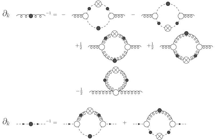
Figure 1: Flow equations for the propagators. Filled circles denote full propagators, open circles correspond to full vertices, and crossed circles indicate the $\partial_{t}R_{k}$-operator insertion.

In the following, we will consider truncations where the Lorentz and color index structures of the vertices are kept identical to the bare ones:

$$V_{\bar{C}AC,\mu}^{abc}(q_{1},q_{2},q_{3}) = f^{abc}q_{1\mu}V_{\bar{C}AC}(q_{1},q_{2},q_{3})$$

$$V_{3A,\mu}^{abc}(q_{1},q_{2},q_{3}) = f^{abc}q_{1\mu}\,V_{3A}(q_{1},q_{2},q_{3})$$

$$V_{4A}^{abcd}(q_{1},\dots,q_{4}) = f^{eab}f^{ecd}\,V_{4A}(q_{1},\dots,q_{4}).$$ (11)

Here $V_{\bar{C}AC},V_{3A},V_{4A}$ are functions of the momentum invariants of $q_{i\mu}$, examples of which will be given later; the bare-vertex truncation is defined by $V_{\bar{C}AC}=V_{3A}=V_{4A}=1$ up to RG rescalings of the fields (cf. Appendix C).

Even though exact solutions of the flow equation are independent of the choice of the regulator, approximate solutions do generally depend on the specific form of $R$. A careful choice of the regulator improves numerical stability as well as the quality of the truncation in general [35]. Here we concentrate on regulators of the type

$$R_{A}(p^{2})=\left(\frac{p^{2}}{Z(p^{2})}\,P_{\text{T}}{}(p)+\frac{p^{2}}{Z_{\text{L}}(p^{2})}\,P_{\text{L}}{}(p)\right)\,r_{A}(p^{2}/k^{2}),\quad R_{C}(p^{2})=\frac{p^{2}}{G(p^{2})}\,r_{C}(p^{2}/k^{2}).$$ (12)

The dimensionless regulator shape function $r_{A,C}(\hat{x})$ with a dimensionless argument determines the analytic form of the momentum space regularization. In addition, we have included the dressing functions in the regulator. In the first place, this construction guarantees that the flow equations are invariant under RG rescaling [36]. Moreover, since we expect a fast RG running of many couplings in the nonperturbative domain, the inclusion of the dressing functions accounts for an adjustment of the regulator to the spectral flow of quantum fluctuations [26, 37, 38].

Let us now introduce some notation in order to facilitate a more explicit representation of the flow equation for the propagators. First we specify squared momentum variables, $x,y,z$, involving the external momentum $p$ and the loop momentum $q$,

$$x=p^{2},\quad y=q^{2},\quad z=(p-q)^{2}=x+y-2u\sqrt{xy},\quad(\hat{x},\hat{y},\hat{z})=(x,y,z)/k^{2},$$ (13)

where $u:=p.q/(|p||q|)$ denotes an angle variable. Here and in the following all hatted quantities are dimensionless by appropriate rescaling with $k^{2}$. Although we are interested in $D=4$ dimensional spacetime in this work, it is worthwhile for future application to perform the computation in arbitrary $D$ dimensional spacetime. For this, we need the $D$ dimensional loop integral of an arbitrary function of $x,y,u$:

$$\int\frac{d^{D}q}{(2\pi)^{D}}\,f(x,y,u) = \tilde{v}_{D}\,\int_{0}^{\infty}dy\,y^{\frac{D}{2}-1}\int_{-1}^{1}du\,(1-u^{2})^{\frac{D-3}{2}}\,f(x,y,u),$$ (15)

$$\tilde{v}_{D}=\frac{2}{\sqrt{\pi}}\,\frac{\Gamma(\frac{D}{2})}{\Gamma(\frac{D}{2}-\frac{1}{2})}\,v_{D},\quad v_{D}=\frac{1}{2^{D+1}\pi^{D/2}\,\Gamma(D/2)}.$$

Here $v_{D}$ is related to the surface volume of a $D$ dimensional sphere $S^{D-1}$. In order to display all dimensionful quantities in terms of $k^{2}$, it is also useful to introduce the dimensionless coupling $\hat{g}_{\Lambda}$,

$$\hat{g}_{\Lambda}^{2}=g_{\Lambda}^{2}\,k^{D-4},$$ (16)

where $g_{\Lambda}$ denotes the value of the coupling at an initial high scale $\Lambda$.

After insertion of this specific regulator form given above, the flow equation for the inverse transverse gluon propagator $\Gamma^{(2)}_{k,AA}(p^{2})=p^{2}/Z(p^{2})+{m}_{k}^{2}$ can be written as

$$\partial_{t}\left(\frac{x}{Z(x)}+{m}_{k}^{2}\!\right) = -4\hat{g}_{\Lambda}^{2}N_{\text{c}}\tilde{v}_{D}k^{2}\int_{0}^{\infty}d\hat{y}\,\hat{y}^{\frac{D}{2}-1}\int_{-1}^{1}du\,(1-u^{2})^{\frac{D-3}{2}}$$

$$\qquad\times\bigg{[}Q^{Z,Z}(\hat{x},\hat{y},u)\,K_{\text{reg}}^{Z,Z}(\hat{x},\hat{y},u)\,V_{3A}\,Z(\hat{y}k^{2})Z(\hat{z}k^{2})\,V_{3A}$$

$$\qquad\qquad\quad+Q^{G,G}(\hat{x},\hat{y},u)\,K_{\text{reg}}^{G,G}(\hat{x},\hat{y},u)\,V_{\bar{C}AC}\,G(\hat{y}k^{2})G(\hat{z}k^{2})V_{\bar{C}AC}\bigg{]}$$

$$-4\frac{(D-1)^{2}}{D}\hat{g}_{\Lambda}^{2}N_{\text{c}}v_{D}\,k^{2}\int_{0}^{\infty}d\hat{y}\,\hat{y}^{\frac{D}{2}-1}$$

$$\qquad\qquad\times\frac{Z(\hat{y}k^{2})}{p_{A}(\hat{y})}\,\bigg{(}-\hat{y}^{2}r_{A}^{\prime}(\hat{y})-\frac{1}{2}\hat{y}r_{A}(\hat{y})\partial_{t}\ln Z(\hat{y}k^{2})\bigg{)}\,V_{4A},$$

where the last term is the tadpole contribution. Since we are ultimatly aiming at the Landau gauge, we have omitted any contribution of the longitudinal modes on the right-hand side of the flow equation which decouple in this limit. The flow equation for the inverse ghost propagator $\Gamma^{(2)}_{k,\bar{C}C}(p^{2})=p^{2}/G(p^{2})$ then yields

$$\partial_{t}\frac{x}{G(x)} = 2\hat{g}_{\Lambda}^{2}N_{\text{c}}\tilde{v}_{D}k^{2}\!\int_{0}^{\infty}\!\!d\hat{y}\,\hat{y}^{\frac{D}{2}-1}\!\int_{-1}^{1}\!\!du\,(1-u^{2})^{\frac{D-3}{2}}\bigg{[}Q^{G,Z}(\hat{x},\hat{y},u)\,K_{\text{reg}}^{G,Z}(\hat{x},\hat{y},u)$$ (18)

$$\qquad\qquad\qquad\qquad\qquad\qquad\qquad\,\times V_{\bar{C}AC}\,G(\hat{y}k^{2})Z(\hat{z}k^{2})\,V_{\bar{C}AC}\!\bigg{]}\!.$$

The quantities $Q^{Z,Z}$, $Q^{G,G}$ denote the kernels of the gluon and ghost loop, respectively, in the gluon flow equation, whereas $Q^{G,Z}$ represents the ghost equation kernel. These kernels are given in Appendix A.

The quantity $K_{\text{reg}}$ abbreviates the contribution from the regularized propagators which reads:

$$K_{\text{reg}}^{Z_{a},Z_{b}}(\hat{x},\hat{y},u) = \frac{1}{p_{a}(\hat{y})p_{b}(\hat{z})}\bigg{[}\frac{-\hat{y}^{2}r_{a}^{\prime}(\hat{y})-\frac{1}{2}\hat{y}r_{a}(\hat{y})\partial_{t}\ln Z_{a}(\hat{y}k^{2})}{p_{a}(\hat{y})}$$ (19)

$$\qquad\qquad\qquad+\frac{-\hat{z}^{2}r_{b}^{\prime}(\hat{z})-\frac{1}{2}\hat{z}r_{b}(\hat{z})\partial_{t}\ln Z_{b}(\hat{z}k^{2})}{p_{b}(\hat{z})}\bigg{]},$$

where the prime denotes a derivative with respect to the argument. Here $Z_{a,b}$ denote gluon and ghost dressing functions, $Z(p^{2})$ and $G(p^{2})$, and $p_{a,b}$ abbreviate the corresponding regularized inverse propagators,

$$p_{C}(\hat{y})=\hat{y}\>(1+r_{C}(\hat{y})),\quad p_{A}(\hat{y})=\hat{y}\>(1+r_{A}(\hat{y}))+Z(\hat{y}k^{2})\>{m}_{k}^{2}/k^{2}.$$ (20)

An explicit expression for the regulator shape function can be found in Appendix B.

Note that all scale derivatives $\partial_{t}\equiv k(d/dk)$ that occur are taken at fixed dimensionful external momentum, $\partial_{t}x=0=\partial_{t}(\hat{x}k^{2})$, so that the scale derivatives on both sides of the flow equation have the same meaning. However, on internal momentum variables the scale derivative acts on the manifest $k^{2}$ dependence, $\partial_{t}\hat{y}=0$. This implies the somewhat clumsy differentiation rule for the dependent momentum variable $\partial_{t}(\hat{z}k^{2})=2\hat{y}k^{2}-2u\sqrt{\hat{y}k^{2}x}$.

Equations (3.2) and (18) represent a closed set of equations for the gluon and ghost propagators in the Landau gauge. Once we have specified initial conditions for $Z$ and $G$ at, say, a perturbative UV scale $k=\Lambda$, we can integrate the flow equations down to $k=0$ and read off the form of the fully dressed propagators. However, before we do so, we first have to discuss the issue of gauge invariance.

3.3 Gauge invariance

Since we are working in a gauge-fixed formulation of Yang-Mills theory, gauge invariance of the system is encoded in a constraint for the effective action. This constraint can either be formulated as a Ward-Takahashi identity or, invoking the BRST formalism, as a Slavnov-Taylor identity. In addition to the breaking of gauge invariance by the gauge-fixing procedure, the regulator term (7) represents another source of gauge or BRST symmetry breaking. In order to account for this additional breaking, both the Slavnov-Taylor and the Ward-Takahashi identity are modified by further terms depending on the regulator. These guarantee the restoration of gauge invariance in the limit $k\rightarrow 0$. The BRST formalism in the flow equation framework has been worked out in Refs. [24, 40, 41]. Since the resulting equation is important for the results of the present paper, we rederive the same findings from the Ward-Takahashi identity here, following [42].

Using the momentum-space representation of the generator $\mathcal{G}^{a}$ of infinitesimal gauge transformations formulated in terms of unrenormalized coupling $g_{0}$ and the fields $A_{0\mu}^{a},C^{a}_{0},\bar{C}^{a}_{0}$ which occur in the microscopic action $S$,

$$\mathcal{G}^{a}(p)=\text{i}p_{\mu}\frac{\delta}{\delta A_{0\mu}^{a}(-p)}-g_{0}f^{abc}\int_{q}\left[A_{0\mu}^{c}(q)\frac{\delta}{\delta A_{0\mu}^{b}(q-p)}+C_{0}^{c}(q)\frac{\delta}{\delta C_{0}^{b}(q-p)}+\bar{C}_{0}^{c}\frac{\delta}{\delta\bar{C}_{0}^{b}(q+p)}\right],$$ (21)

the modified Ward-Takahashi identity (mWTI) for covariant gauges can be written as

$$\mathcal{G}^{a}(p)\left[\Gamma_{k}-\int\left(\frac{1}{2\xi}(\partial_{\mu}A_{0,\mu}^{a})^{2}+(\partial_{\mu}\bar{C}_{0}^{a})D_{\mu}^{ab}(A_{0})C_{0}^{b}\right)\right]$$

$$\quad=-\frac{1}{\xi}g_{0}f^{abc}\int_{q}(p+q)_{\mu}(p+q)_{\nu}\langle A_{0,\mu}^{c}(-q)A_{0,\nu}^{b}(p+q)\rangle_{\text{con}}$$

$$\qquad-g_{0}f^{abc}\int_{q_{1},q_{2}}p_{\mu}\big{(}\delta(p+q_{1}-q_{2})q_{2\mu}\delta^{bf}-\text{i}g_{0}f^{bef}A_{0,\mu}^{e}(p+q_{1}-q_{2})\big{)}\langle\bar{C}_{0}^{c}(q_{1})C_{0}^{f}(q_{2})\rangle_{\text{con}}$$

$$\qquad-\text{i}g_{0}^{2}f^{abc}f^{feb}\int_{q_{1},q_{2}}p_{\mu}\langle\bar{C}_{0}^{c}(q_{1})A_{0,\mu}^{e}(p+q_{1}-q_{2})C_{0}^{f}(q_{2})\rangle_{\text{con}}$$

$$\qquad-\frac{1}{2}g_{0}f^{abc}\int_{q}\big{[}R_{A,\mu\nu}(p+q)-R_{A,\mu\nu}(q)\big{]}\langle A_{0,\mu}^{c}(-q)A_{0,\nu}^{b}(p+q)\rangle_{\text{con}}$$

$$\qquad-g_{0}f^{abc}\int_{q}\big{[}R_{C}(p+q)-R_{C}(q)\big{]}\langle\bar{C}_{0}^{c}(q)C_{0}^{b}(q+p)\rangle_{\text{con}},$$ (22)

where the first four lines represent the standard Ward-Takahashi identity, and the last two lines are the modification owing to the regulator. In the limit $k\to 0$, the regulator terms vanish such that the standard WTI is recovered. The important observation is that the mWTI is compatible with the flow equation in the sense that if a solution of the flow equation satisfies the mWTI at one scale, it does so for all scales. Hence, if our initial conditions at the high scale satisfy the mWTI at $k=\Lambda$, the end point of the RG trajectory at $k\to 0$ which is the full quantum effective action will be gauge invariant, i.e., will fulfill the standard WTI. However, these statements only hold for the full effective action. A truncated flow can leave the gauge-invariant trajectory which is constrained by the mWTI. In order to satisfy the symmetry principle encoded in the mWTI, the degrees of freedom in the truncation can be subdivided into truly independent ones, the dynamics of which is determined by the flow equation, and the dependent ones that can be expressed in terms of independent degrees of freedom by virtue of the mWTI. In this way, the symmetry principle is satisfied on the theory subspace defined by the truncation, and gauge invariance is consistently implemented within the truncation [40, 43].

In the present truncation, the mWTI first of all constrains the longitudinal gluon propagator. Although the longitudinal components decouple in the Landau gauge which we are aiming at, the mWTI nevertheless provides an important piece of information. Evaluating Eq. (22) in the zero-momentum limit of the longitudinal propagator, the mWTI constrains the value of the gluon mass $m_{k}$. In order to represent this constraint for the gluon mass in terms of the quantities appearing in our truncation (10), we need to know the relation between the fields $(A_{0},\bar{C}_{0},C_{0})$ appearing in $\mathcal{G}^{a}$ and the fields renormalized at the scale $\Lambda$ in which the effective action is expressed, i.e., we need to determine the renormalization factors $Z_{A}$ and $Z_{C}$ defined by

$$A_{0\mu}=\sqrt{Z_{A}}A_{\mu},\quad(\bar{C}_{0},C_{0})=\sqrt{Z_{C}}\,(\bar{C},C).$$ (23)

The connection between the renormalization factors in the exact RG approach and the conventional $\overline{\text{MS}}$ scheme have been worked out in Ref. [44]. Identifying $\Lambda$ with the renormalization scale, the boundary conditions for the flow at $\Lambda$ are equivalent to renormalization conditions in the $\overline{\text{MS}}$ scheme, and the finite parts of the respective renormalization factors can be related to each other.

As will be detailed in Sect. 4.1, our initial effective action at $\Lambda$ will be obtained by integrating the bare action $S_{\text{YM}}+\Delta S_{k}$, Eqs.(6,7), from an even larger scale $\Lambda_{\text{UV}}$ down to $\Lambda$. With

$$1=Z_{T,\Lambda_{\text{UV}}}(0)=Z_{\Lambda}(0)Z_{A}(\Lambda),\quad 1=G_{\Lambda_{\text{UV}}}(0)=G_{\Lambda}(0)Z_{C}(\Lambda),$$ (24)

we then obtain

$$A_{\mu}=\sqrt{Z_{\Lambda}(0)}A_{0\mu},\quad(\bar{C},C)=\sqrt{G_{\Lambda}(0)}\,(\bar{C}_{0},C_{0}),$$ (25)

where $(Z_{\Lambda}(p^{2}),G_{\Lambda}(p^{2}))=\lim_{k\to\Lambda}(Z(p^{2}),G(p^{2}))$. Furthermore, the nonperturbative definition of the running coupling, Eq. (4), gives the relation

$$g_{0}^{2}=g_{\Lambda}^{2}\,G_{\Lambda}^{2}(0)Z_{\Lambda}(0).$$ (26)

With these relations the mWTI for the gluon mass yields [26]

$$m_{k}^{2}\!\!\! = \!\!\!\frac{8}{D}v_{D}\hat{g}_{\Lambda}^{2}N_{\text{c}}\,G_{\Lambda}(0)\,k^{2}\int_{0}^{1}d\hat{y}\,\hat{y}^{D/2-1}\Bigg{\{}V_{\bar{C}AC}\,G(\hat{y}k^{2})\frac{(-\hat{y}^{3}r_{C}^{\prime}(\hat{y}))}{p_{C}^{3}(\hat{y})}+(D\!-\!1)\frac{V_{3A}\,Z(\hat{y}k^{2})}{p_{A}^{2}(\hat{y})}$$

$$\!\!\!\times\left[\frac{D\!-\!1}{4}\hat{y}r_{A}(\hat{y})+\frac{\hat{y}^{3}r_{A}^{\prime}(\hat{y})}{p_{A}(\hat{y})}+\frac{Z(\hat{y}k^{2})m_{k}^{2}}{k^{2}}\frac{(\hat{y}^{2}r_{A}^{\prime}(\hat{y})+\hat{y}r_{A}(\hat{y}))}{p_{A}(\hat{y})}+\frac{Z^{\prime}(\hat{y}k^{2})m_{k}^{2}}{k^{2}}\frac{\hat{y}^{2}r_{A}(\hat{y})}{p_{A}(\hat{y})}\!\right]\!\!\!\Bigg{\}}\!,$$

where we have again dropped longitudinal contributions on the right-hand side according to the Landau gauge, and primes denote a derivative with respect to $\hat{y}$. The occurrence of the gluon mass $m_{k}$ is an obvious consequence of gauge-symmetry breaking by the regulator. Assuming that the dressing functions diverge, if at all, with a simple power or weaker $V_{3A}Z(p^{2}),V_{\bar{C}AC}G(p^{2})\lesssim(1/p^{2})^{\kappa}$ in the IR limit, the $k$ dependence of the mass is bounded by $m_{k}^{2}\lesssim(k^{2})^{1-\kappa}$ towards the IR. Removing the regulator with $k\to 0$, the mass vanishes as long as $\kappa<1$. Therefore, $\kappa<1$ serves as a consistency condition that our solutions have to obey in order to satisfy the standard WTI in the present truncation.

Since the gluon mass also appears on the right-hand side of Eq. (LABEL:mWTIm), the mWTI represents a “gap” equation for a self-consistent determination of the gluon mass. Moreover, the RG evolution of this mass is completely determined by the evolution of $Z$ and $G$ and the vertices. In this way, the mWTI guarantees that the gluon mass is not an RG relevant parameter, as is conventionally the case for boson masses, but RG irrelevant, since it drops to zero with $k\to 0$.

On the other hand, from the flow equation for the transversal gluon propagator (3.2), we can read off the flow of the gluon mass in the zero-momentum limit. Of course, for the exact solution, this mass flow would fully agree with that of the mWTI; both mass equations also agree in the perturbative limit of the truncation ($G,Z\to\,$const., $V_{\bar{C}AC,3A,4A}\to 1$), which serves as a nontrivial check of the approach [26]. Nonperturbatively, however, both equations for the mass can differ strongly, even qualitatively, since an exact implementation of the gauge constraint always requires information which is beyond the truncation. The gluon mass is particularly sensitive to this fact, since any deviation from a gauge-invariant RG trajectory can lift its protection against quadratic renormalization (as can occur for massive bosons); then, the gluon mass would be of the order of the cutoff, $m_{k}^{2}\sim\Lambda^{2}$. Indeed, this is what would happen if we took the mass flow of the transversal gluon seriously, disregarding the mWTI. In similar truncations of DSEs, the very same fact occurs as quadratic divergencies in the gluon equation which have to be removed by hand. In the context of flow equations, we have the mWTI at our disposal for controlling the mass flow. For this, we subtract the mass flow from the transversal gluon equation and put in the mass from the mWTI:

$$\partial_{t}\frac{x}{Z(x)}=\text{RHS~{}(\ref{fm1})}\big{|}_{m_{k}^{2}\,(\text{mWTI})}-\partial_{t}m_{k}^{2}\big{|}_{\text{flow}}=\text{RHS~{}(\ref{fm1})}\big{|}_{m_{k}^{2}\,(\text{mWTI})}-\text{RHS~{}(\ref{fm1})}|_{x\to 0},$$ (28)

where the gluon mass in the RHS is taken from the mWTI. For the exact solution, Eq. (28) corresponds to a zero operation, whereas in the truncation, this procedure removes quadratically renormalizing parameters by virtue of the gauge constraint.

4 Flow analysis

In this section, we analyze the flow equation partly analytically but mainly numerically for various initial conditions and truncations. We concentrate on the case of $D=4$ dimensional spacetime and $N_{\text{c}}=3$ colors unless stated otherwise. In the next subsection we will specify two different types of boundary conditions at large and intermediate momenta that serve as initial conditions for the flow. We proceed by analyzing the RG equations analytically on a qualitative level and determine conditions for the higher n-point functions such that the IR attractive power-law domain can be approached by the flow. Guided by these findings, we then perform a numerical analysis of the flow in various truncation schemes. The details of our numerical methods are given in Appendix D.

4.1 Initial conditions

The solution of a quantum theory is determined by the RG flow equation and the corresponding initial conditions. For the latter, we have to specify the details of the initial effective action $\Gamma_{\Lambda}$, serving as our boundary condition at the scale $\Lambda$. For a perturbatively small coupling $g_{\Lambda}$ at $\Lambda$, one could choose the bare action (6) for $\Gamma_{\Lambda}$. Improved initial conditions can be obtained by perturbatively integrating the flow equation from a larger scale $\Lambda_{\text{UV}}$ down to $\Lambda$, employing bare dressing functions on the right-hand side of the flow equation. This guarantees the correct one-loop behavior of the dressing functions and subsequently of the running coupling for momenta $p^{2}\gg\Lambda$ far larger than our starting scale. Of course, a correct matching to the full flow at $\Lambda$ requires the inclusion of the regulator function $R_{k}$ in this perturbative determination of the initial conditions. Qualitatively, the high-momentum behavior, $p^{2}\gg\Lambda^{2}$, of the dressing functions for one-loop improved perturbative initial conditions (PIC) is

$$Z^{\text{PIC}}(p^{2})|_{\Lambda}\simeq Z_{\Lambda}\left(1+\gamma_{A}\,\frac{11}{N_{\text{c}}\alpha_{\Lambda}}{12\pi}\ln\frac{p^{2}}{\Lambda^{2}}\right),\quad G^{\text{PIC}}(p^{2})|_{\Lambda}\simeq G_{\Lambda}\left(1+\gamma_{C}\,\frac{11}{N_{\text{c}}\alpha_{\Lambda}}{12\pi}\ln\frac{p^{2}}{\Lambda^{2}}\right),$$ (29)

where $\gamma_{A}=-13/22$ and $\gamma_{C}=-9/44$ denote the anomalous dimensions for gluons and ghosts, respectively, for arbitrary $N_{\text{c}}$, and $Z_{\Lambda},G_{\Lambda}=Z(\Lambda^{2}),G(\Lambda^{2})|_{\Lambda}$ denote the normalizations of the fields. For low momenta $p^{2}\ll\Lambda^{2}$, the perturbative initial conditions for the dressing functions go to a constant, owing to the presence of the regulator.

Certainly, universality tells us that such a one-loop RG improvement is irrelevant for the questions related to the IR behavior. Whether a truncation is good enough to stabilize the flow in the mid-momentum regime between the perturbative UV and the deep IR should not depend on the details of the UV behavior of the initial effective action. We have confirmed that this is indeed not the case, employing both a bare initial action and its one-loop improved counterpart.

Since it turns out that a full solution connecting perturbative initial conditions with the expected IR behavior is difficult to construct, we design instead a set of mid-scale initial conditions for exploring in particular the flow in the nonperturbative IR regime. For this, we consider the initial scale $\Lambda$ to be already in the nonperturbative regime but still high enough such that the IR asymptotics has not yet developed, say, for instance, $\Lambda\gtrsim 1$GeV. For definiteness, we study two contrary cases: one in which the ghost dressing function has already developed a scale $L$, whereas the gluon remains perturbative (or even constant),

$$G^{(\eta_{C})}(p^{2})|_{\Lambda}=G_{\Lambda}\,\left(\frac{p^{2}}{L^{2}+p^{2}}\right)^{\eta_{C}},\quad Z^{(\eta_{C})}(p^{2})|_{\Lambda}=Z_{\Lambda}.$$ (30)

Here, $\eta_{C}$ denotes a trial exponent to be varied, and the scale $L$ separates perturbative from deep IR behavior. The other case is given by a scale in the gluon dressing function and a perturbative ghost,

$$G^{(\eta_{A})}(p^{2})|_{\Lambda}=G_{\Lambda},\quad Z^{(\eta_{A})}(p^{2})|_{\Lambda}=Z_{\Lambda}\,\left(\frac{p^{2}}{L^{2}+p^{2}}\right)^{\eta_{A}}.$$ (31)

For a trial gluon power $\eta_{A}\sim 1$, the scale $L$ plays the role of a nonperturbative gluon mass. Such a nonperturbative gluon mass should not be confused with the mass $m_{k}$ controlled by the WTI, cf. subsection 3.3. In general, the scale $L$ will survive when the IR cutoff $k$ is taken to zero, whereas $m_{k}\rightarrow 0$ in this limit according to the WTI.

Note that Eqs. (30) and (31) are initial conditions at a fixed mid-momentum scale, and do not represent an ansatz for the form of the dressings at even lower scales. In other words, we will determine the resulting full momentum dependence at lower scales and not merely the flow of the parameters $\eta_{A,C}$ and $L$.

The use of these mid-scale initial conditions  (30), (31) for the IR flow facilitates a study of the IR attractive domain of the asymptotic power solutions obtained so far in the literature. In this way, we can analyze the necessary ingredients for a solution of the flow at an intermediate scale $k$ to finally run into the power-law solutions for $k\to 0$; it dispenses us from the need to solve the complete flow from the UV to the IR in particular in the transition region, where vertex corrections are expected to become important.

4.2 Qualitative analysis

Some important features of the present set of RG equations for the propagators can already be extracted by a qualitative analysis. We begin with the observation that the perturbative initial conditions  (29) are such that the dressing functions are increasing functions for decreasing momentum $p^{2}=x$. In view of the expected IR behavior $G(x)\sim x^{-\kappa}$ with $\kappa\gtrsim 0.5$ (cf. Sect. 2), this property should persist and even be enhanced for the ghost dressing. By contrast, the gluon dressing is expected to decrease in the IR with $Z(x)\sim x^{2\kappa}$, such that the flow equation has to bend the gluon dressing in the IR.

Let us check the ghost equation (18) first. As long as the vertex dressing $V_{\bar{C}AC}$ remains positive, the RHS of the ghost flow is strictly positive; particularly, the kernel $Q^{G,G}$, given in Appendix A, and the dressing functions are positive. The first term in the regulator quantity $K_{\text{reg}}$ is positive as $r^{\prime}(\hat{y})<0$ for all monotonous regulator shape functions, like the one specified in Eq. (D.7) below. Moreover, the mechanism for a sign change should not depend on the details of the regulator. The other terms $\sim\partial_{t}\ln Z_{a}$ in $K_{\text{reg}}$ are positive for perturbative initial conditions, and thus they cannot induce a sign change, owing to the $\partial_{t}$ structure. Regarding the RHS of the ghost equation as “$\beta$ functions” for a set of “couplings” $x/G(x)$ labeled by $x$, the positivity of these “beta functions” guarantees that the “couplings” decrease towards the IR. Consequently, this decrease of $x/G(x)$ with $k\to 0$ implies an increase of $G(x)$ towards the IR. This is consistent with the IR expectation of an enhanced ghost, $G(x)\sim x^{-\kappa}$.

Next we apply this argument to the gluon equation (3.2). Since we anticipate a suppression of $Z(x)$ for small $x$, we need a negative “$\beta$ function” for $x/Z(x)$. Hence, we expect a negative RHS for small $x$, once we have subtracted the gluon mass flow $\partial_{t}m_{k}^{2}$ in order to isolate the flow of $x/Z(x)$. Let us analyze Eq. (3.2) term by term, beginning with the gluon loop with kernel $Q^{Z,Z}$. For simplicity, we consider first the limit of $x\ll k^{2}$ where the propagator and vertex dressings as well as $K_{\text{reg}}$ become rather independent of $x$, owing to the regularization (the $\hat{z}$ dependence can safely be replaced by $\hat{y}$ in these quantities). Hence the sign of the kernel after mass flow subtraction determines the overall sign. Using representation (A.1), this corresponds to

$$Q^{Z,Z}(\hat{x},\hat{y},u)-Q^{Z,Z}(0,\hat{y},u)=-(1-u^{2})\left[\hat{x}+\frac{\hat{x}\hat{y}}{\hat{z}}\left(1-\frac{1-u^{2}}{D-1}\right)\right]\leq 0.$$ (32)

Together with the overall minus sign in Eq. (3.2), we find that the gluon loop contribution to the “$\beta$ function” is positive. Hence $x/Z(x)|_{\text{gluon loop}}$ decreases towards the IR, implying that $Z(x)|_{\text{gluon loop}}$ increases. We have derived this result in the limit $x\ll k^{2}$; but owing to the regularization, a well-converging expansion of the flow in $x/k^{2}$ exists, such that the validity of this statement can be extended to $x\lesssim k^{2}$. Even within the limits of these mild assumptions, we arrive at an important first result: the gluon loop in the gluon equation cannot be the source of a bending and a subsequent suppression of the gluon dressing. This statement holds for all 3-gluon vertex dressings that are non-negative and preserve the bare-vertex index structure.

Now we turn to the ghost-loop contribution to the gluon equation with kernel $Q^{G,Z}$. The situation here is more subtle, since the kernel is independent of $x$ (see Eq. (A.2)), such that the residual terms after mass-flow subtraction arise from the $\hat{z}$-dependent ghost and vertex dressings and $K_{\text{reg}}$. Collecting all these $\hat{z}$ dependencies in a function $f(\hat{z})\sim V_{\bar{C}AC}G(\hat{z}k^{2})K_{\text{reg}}$, we have to study the sign of ($\hat{z}|_{x\to 0}=\hat{y}$):

$$f(\hat{z})-f(\hat{y})=\hat{x}f^{\prime}(\hat{y})+\mathcal{O}(\hat{x}^{2}),$$ (33)

where we have dropped all terms odd in $u$ that are canceled by the $u$ integration. $G(p^{2})$ as well as $K_{\text{reg}}$ for generic regulator shape functions are decreasing functions of the momentum. In the bare-vertex truncation $V_{\bar{C}AC}=1$, the RHS of Eq. (33) is therefore negative for small $\hat{x}$, because $f^{\prime}(\hat{y})\leq 0$. Together with the overall minus sign of Eq. (3.2), this again implies a positive “$\beta$ function” and thus a contribution to the flow of $Z(x)$ that cannot suppress the dressing function in the IR. This statement is, of course, weaker than the one given above for the gluon loop, since a non-negative ghost-gluon vertex dressing can, in principle, turn the sign of $f^{\prime}(\hat{y})$. However, this would be an unexpected source for the bending of the gluon dressing, since the ghost loop is not anticipated to play a dominant role at intermediate scales.

Let us finally continue our discussion with the tadpole contribution in Eq. (3.2). For a bare-vertex truncation $V_{4A}\to$ const., the tadpole does not contribute at all to the flow of $Z(x)$, but only to the mass flow. However, as soon as the 4-vertex acquires a nontrivial momentum dependence under the flow, the tadpole can contribute with either sign. Especially if the vertex dressing decreases with external momentum $x$, its “$\beta$ function” contribution can be negative, thereby inducing a suppression of the gluon in the IR.

To summarize, a vertex expansion of the effective action has the potential to describe Landau-gauge ghost enhancement and gluon suppression in agreement with, e.g., lattice results. A realization of this scenario in a truncation on the 3-vertex level requires exceptional (i.e., negative) vertex dressings or suitable index structures beyond the bare ones. By contrast, a truncation including dressed 4-vertices can accommodate gluon suppression more conventionally with merely positive vertex dressings and bare index structures.

4.3 Vertices

Since we intend to perform a vertex expansion to lowest non-trivial order, we do not attempt to solve the full dynamical equations for the vertices. The choice of the latter hence determines the remaining unspecified part of the truncation. Basically three different strategies can be pursued: first, the highest vertices in a vertex expansion can be taken as bare. Second, these vertices can be computed self-consistently from their truncated dynamical equations. These first two strategies define a consistent approximation scheme generalizable to higher orders. Third, the vertices can be modeled employing further physical information.

In the literature, the second strategy of deriving or at least constraining vertices by their truncated equations has been frequently followed. In particular in gauge theories, the constraints from the Ward-Takahashi or Slavnov-Taylor identities can serve as an additional input and have been exploited in [26, 28, 4]. However, it still remains unclear whether this strategy can be successful, since the truncated equations may lack important structural information from the neglected terms; in fact, this manner of construction can even lead to inconsistencies as exemplified in [5, 6, 46].

In this work, we use a set of different vertices in order to explore different routes that the flow can take from the UV to the IR. First of all, the ghost-gluon vertex is taken to be bare, $V_{\bar{C}AC}=1$, which is in agreement with the non-renormalization property (3) but neglects possible finite renormalizations. In the gluonic sector, we consider:

• bare 3-gluon vertex, $V_{3A}=G_{\Lambda}/Z_{\Lambda}$, where factors $G_{\Lambda},Z_{\Lambda}$ take the normalization of the fields at $\Lambda$ into account (cf. Appendix C);

• modified bare 3-gluon vertex, $V_{3A}=\rho\,G_{\Lambda}/Z_{\Lambda}$, where the possibly $k$-dependent parameter $\rho$ can be varied in order to suppress or enhance the 3-gluon vertex; we will especially make use of a vertex suppression with $\rho$ becoming gradually smaller than 1, in agreement with recent lattice results [47]. An exceptional case is given by $\rho=0$: the “ghost-loop-only” truncation;

• dressed 3-gluon vertex,

  $$V_{AAA}=\frac{1}{G(q^{2})^{1+3\delta}\,Z(q^{2})^{(1+3\delta)/2}}\,\frac{1}{G((p-q)^{2})^{1+3\delta}\,Z((p-q)^{2})^{(1+3\delta)/2}},$$ (34)

  where $q^{2}$ and $(p-q)^{2}$ denote the momenta running around the loop, and $\delta=-9/44$ is the anomalous dimension of the ghost dressing function to one-loop order. This type of vertex construction has been used in the DSEs to ensure the correct one-loop anomalous dimensions of the ghost and gluon dressing functions in the UV [8]. Since it breaks RG scaling invariance explicitly in the nonperturbative momentum regime, rescaling the initial conditions for the fields with $G_{\Lambda},Z_{\Lambda}$ corresponds to suppressing or enhancing this vertex analogous to (b);

• bare 4-gluon vertex $V_{4A}=G_{\Lambda}^{2}/Z_{\Lambda}$. However, since the 4-gluon vertex occurs only in the tadpole diagram, the bare-4-gluon vertex truncation is identical to the no-4-gluon-vertex truncation, since the momentum-independent part of the tadpole contributes only to the mass flow and thus is subtracted completely;

• dressed 4-gluon vertex,

  $$V_{4A}=G^{\gamma_{1}}(p^{2})G^{\gamma_{2}}(r^{2})\,Z^{\zeta_{1}}(p^{2})Z^{\zeta_{2}}(r^{2}),\quad\gamma_{1}+\gamma_{2}=2,\quad\zeta_{1}+\zeta_{2}=-1,$$ (35)

  where $p^{2}$ denotes the external momentum, and $r^{2}$ can be set equal to the internal momentum $q^{2}$ or other scales such as $k^{2}$ or $\Lambda^{2}$. The constraints for the exponents $\gamma_{i}$, $\zeta_{i}$ arise from RG rescaling invariance.

4.4 Numerical results

4.4.1 Perturbative initial conditions and bare vertices

Here we solve the flow from the perturbative UV towards the IR, imposing one-loop improved initial conditions. For illustration, we start the flow at $\Lambda=M_{Z}=91.187$ GeV with $\alpha(M_{Z})=0.118$.

Our results for the bare-vertex truncation are shown in Fig. 2. In agreement with our analysis of Sect. 4.2, both dressing functions increase towards the IR. After a few orders of magnitude of perturbative running, the flow in fact becomes singular at a finite scale $k_{\text{sing}}$ where the gluon dressing diverges. As a consequence, the coupling $\alpha$ also diverges reminiscent of the Landau-pole singularity of perturbation theory.

     

Figure 2: Numerical results for ghost and gluon dressing functions and the running coupling employing the bare vertex truncation. Left panel: bare 3-gluon vertex (a). Right panel: modified bare 3-gluon vertex (b) with $\rho$ decreased from 1 to 0.2. Both flows become singular at a finite value of $k$, signaling the breakdown of the oversimplified truncation. The coupling exhibits a singularity of Landau-pole type. Other multiplicative positive 3-gluon vertex dressings lead to similar results.

This singular behavior of the gluon is mainly driven by the gluon loop involving the 3-gluon vertex. Since the latter is expected to be suppressed in the IR, let us use the modified bare 3-gluon vertex with a suppression parameter of $\rho<1$. On the left panel of Fig. 2, we show the flow for this truncation with $\rho$ gradually decreased from 1 to 0.2 for decreasing $k$. Though the gluon dressing now remains finite, it is the ghost dressing that diverges at finite $k$ and thereby triggers a singularity of Landau-pole type.

These observations are in agreement with the analysis of Sect. 4.2 and stress the fact that a truncation with a multiplicative positive dressing of the 3-gluon vertex is not capable of describing the flow from the perturbative UV to the IR power-law asymptotics.

4.4.2 Perturbative initial conditions with dressed 4-gluon vertex

Let us now include a momentum-dependent 4-vertex dressing of the type (e) in Eq. (35). In agreement with our observations of Sect. 4.2, the truncation now has the potential to describe an IR suppression of the gluon towards the expected IR asymptotics.

In Fig. 3, we display a typical solution for the gluon and ghost dressings, exhibiting IR ghost enhancement and gluon suppression. All solutions look qualitatively similar for vertex parameters $\gamma_{1},\zeta_{1}>0$ in Eq. (35). We also observe a quantitative stability for $\gamma_{1}=\mathcal{O}(1)$ and $\zeta_{1}=0.1\dots 0.5$. (Fig. 3 is computed with $\gamma_{1}=1.1$, $\zeta_{1}=1/2$, $r^{2}=\Lambda^{2}$ and a modified bare 3-gluon vertex (b) with $\rho$ decreasing from 1 to 1/2 in the mid-momentum regime in order to avoid a Landau-type singularity).

Nevertheless, the vertex ansatz (35) appears to be too simple for establishing a full UV-to-IR connection. Although Landau-type singularities can be avoided over the full momentum window that we have studied, we have not discovered an IR asymptotics with a high degree of universality, such as a clear signal of stable power laws for the dressings.

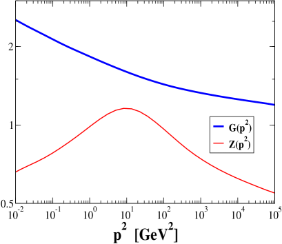
Figure 3: Numerical results for the ghost and gluon dressing functions, including a dressed 4-gluon vertex (e). This truncation is capable of describing ghost enhancement and gluon suppression in the IR. (Vertex parameters: $\gamma_{1}=1.1$, $\zeta_{1}=1/2$, $r^{2}=\Lambda^{2}$, and $\rho=1\dots 1/2$.)

4.4.3 IR flow analysis

Let us now concentrate on the flow of the propagators towards the IR asymptotics. DSE as well as RG flow equation studies have demonstrated that the power-law behavior discussed in the introduction is a self-consistent solution of the dynamical equations in the IR, implying an IR stable fixed point for the gauge coupling. The following study is devoted to an investigation of the domain of attractivity of this fixed point. For this, we assert that the fluctuations from the UV down to an intermediate scale $\Lambda\sim 1$GeV have already modified the dressing functions as compared to their perturbative form in an a priori unknown manner. By assuming various initial conditions for the dressing functions at intermediate $k$ scales, we can check whether the flow connects a particular mid-scale initial condition with the IR fixed point regime and power laws. In this way, we can analyze the mid-momentum requirements that facilitate a full UV – IR connection. This particularly provides information about the physical mechanisms that have to be triggered by the (yet unknown) full vertices. Throughout this subsection, we use bare ghost and 4-gluon vertices – a truncation that is sufficient for the expected IR asymptotics, owing to ghost dominance in the gluon equation. Beyond this, we vary the 3-gluon vertex in order to study its influence on the approach to the IR.

     

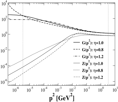
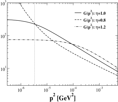
Figure 4: Numerical results for the ghost and gluon dressing functions in the minimally dressed vertex truncation (c), Eq. (34), employing a gluon dressing function with a scale, (31), and a constant ghost as boundary conditions at an intermediate momentum scale. For an initial gluon power in a small but finite interval around $\eta_{A}\simeq 1$, the ghost shows a clear signal for IR power-law asymptotics with $\kappa\simeq 0.52$. The right panel magnifies the IR asymptotics of the ghost of the left panel, demonstrating the failure of the ansätze with $\eta_{A}=0.8$ or $\eta_{A}=1.2$, which are outside the attractive region of the IR-power law solution. (The vertical dotted line indicates the lower end $k_{\text{IR}}$ of the window of $k$ integration.)

Two initial conditions for the ghost and gluon dressing functions at $k=\Lambda$ reflecting opposite situations in the mid-momentum regime have been given in Eq. (30) and (31). In addition to being related to $\Lambda$, both boundary conditions contain a scale $L$ appearing either in the initial ghost or gluon dressing function. Certainly, Yang-Mills theory is governed by only one scale, which is $\Lambda_{\text{QCD}}$. The relation between $\Lambda$ and $\Lambda_{\text{QCD}}$ is uniquely determined by the RG, once the coupling $g_{\Lambda}$ is fixed at $\Lambda$. Such a unique relation also has to exist for $L$, i.e., $L=\text{const.}\times\Lambda_{\text{QCD}}$. To guarantee that our initial condition represents a valid approximation to Yang-Mills theory at our initial scale $\Lambda$, we have to determine this constant. Otherwise our system describes a different theory with two independent scales.

For solving this problem, we note that, once we have found the right value of $L$, the flow in the deep IR will not develop yet another scale and the dressings will depend only on $p^{2}/L^{2}\sim p^{2}/\Lambda_{\text{QCD}}$. On the other hand, a separate dependence of our solutions on $L$ and $\Lambda$ indicate the failure of the initial condition. In practice, instead of tuning $L/\Lambda$ for fixed $g_{\Lambda}$, we keep $L/\Lambda$ fixed, say $L/\Lambda=0.01$, and fine-tune the value of the initial coupling $g_{\Lambda}$ such that no further scale arises in our solutions in the deep IR. Examples of such an additional but unphysical scale are rapid changes, steps or singularities in the dressings.

Let us first investigate the initial condition (30), which assumes that the ghost dressing has already developed a scale, whereas the gluon is taken as perturbative for all momenta $p^{2}$. With these boundary conditions we find that the flow runs into a singularity at finite $k_{\text{sing}}$ independently of the initial ghost exponent $\eta_{C}$ or the value of $L$. The mechanism responsible for such a behavior has been analysed in Sect. 4.2: in the truncation considered here, the gluon cannot develop an IR suppression with $k\rightarrow 0$. Thus an unsuppressed gluon at a mid-momentum scale $k=\Lambda$ drives the flow away from the IR fixed point.

     

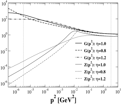
Figure 5: Numerical results for the ghost and gluon dressing functions, employing a gluon dressing function with a scale, (31) and a constant ghost as boundary conditions at an intermediate momentum scale. The left panel shows the result for the modified bare vertex truncation (b) with $\rho=0.5$, a “ghost-loop-only” truncation ($\rho=0$) is displayed on the right panel. Both truncations lead to IR power law asymptotics with $\kappa\simeq 0.52$ if the initial gluon power is in a small but finite interval around $\eta_{A}\simeq 1$.

This is different for the initial condition (31), where we assume that the gluon has already developed a suppression with scale $L$ at $k=\Lambda$ and the ghost remained perturbative. In Fig. 4, we plot the solution of the flow equation for the initial conditions with initial gluon exponent $\eta_{A}=0.8,1.0,1.2$ for the minimally dressed 3-gluon vertex (c), Eq. (34). The regulator scale $k$ has been integrated down to a value $k_{\text{IR}}$ that is indicated by the vertical dotted line on the left-hand side of the plots. For all three values of $\eta_{A}$, the ghost dressings are strongly enhanced in the IR, whereas the gluon develops a more enhanced peak around $L$.

For $\eta_{A}=1$ (solid lines), the ghost dressing exhibits a clear power law, $G(p^{2})\sim(p^{2})^{-\kappa}$, for all momentum values $k_{\text{IR}}^{2}\lesssim p^{2}\lesssim L^{2}$. We identify a ghost exponent of

$$\kappa\simeq 0.52.$$ (36)

The gluon develops a power slightly stronger than its initial power $\eta_{A}$. This behavior is universal for initial powers $\eta_{A}$ in a small but finite interval around $\eta_{A}\simeq 1$, i.e., for boundary conditions in this interval the IR power $\kappa$ does not depend on $\eta_{A}$. As will be discussed in more detail below, this result corresponds to the self-consistent solutions found, for instance, in the IR analysis of DSEs.

For $\eta=1.2$ (dot-dashed lines), a power law in the ghost dressing develops, but not over the full $k$ integration range. At some scale $k^{2}\gg k_{\text{IR}}^{2}$, the ghost gets stuck and becomes essentially perturbative again. Apparently, the gluon is too strongly suppressed to control the build up of a power law to arbitrarily small momenta. Since this solution exhibits a second independent scale where the ghost becomes perturbative again, we conclude that this ansatz with $\eta_{A}=1.2$ fails to describe the IR of Yang-Mills theory.

For $\eta_{A}=0.8$, the ghost first builds up a power law, but then deviates in the IR and runs into a singularity (the plot shows a curve with $g_{\Lambda}$ chosen such as to allow for a maximal IR extension). For this set of initial conditions, the gluon is not suppressed strongly enough in the IR to prevent the same singularity as observed frequently above. We conclude that also this initial condition with $\eta_{A}=0.8$ fails to represent the physics of the IR sector.

These features remain qualitatively the same for the various 3-gluon vertices, unless this vertex is not too strong at intermediate scales. In Fig. 5, we show results for the modified bare vertex (b) with $\rho=0.5$ and a “ghost-loop-only” truncation ($\rho=0$). In agreement with the literature, this reveals the ghost loop as the dominant IR structure, in support of the Kugo-Ojima confinement scenario.

5 Summary and conclusions

We have performed a study of the vertex expansion of the quantum effective action of Landau-gauge Yang-Mills theory in the framework of the exact renormalization group. We have truncated the vertex expansion at the lowest nontrivial order and concentrated on the behavior of the ghost and gluon propagators. This level of truncation already contains important information about large-distance physics along the lines of the Kugo-Ojima confinement criterion.

We identify three different momentum regimes in our investigation: a perturbative high-momentum region, a nonperturbative regime around $p^{2}\sim\mathcal{O}(1)\text{GeV}^{2}$ presumably dominated by gauge field fluctuations and a regime in the deep IR dominated by the ghost degrees of freedom. Simple truncations of the RG flow equation cannot only easily deal with the perturbative regime, but give conclusive answers for the deep IR. In the literature, a power-law behavior of the dressings has been self-consistently determined in the deep IR, which is related to an IR fixed point of the running coupling and realizes the Kugo-Ojima confinement criterion [6, 7, 8, 30].

In addition to these studies, our work analyzes the flow towards this fixed point and explores its domain of attractivity. For this, we employ a set of mid-scale initial conditions for the propagator dressings that may arise from the flow, once the fluctuations at intermediate momenta have also been properly integrated out. Within this set, our results demonstrate that a mass-like structure in the gluon dressing (characterized by an initial gluon power in a small but finite interval around $\eta_{A}\simeq 1$ and a scale $L$) is a necessary prerequisite for approaching the power-law asymptotics in the IR. Other tested mid-scale initial conditions lead to either a singular or a trivial behavior of the propagator dressings. For the mass-like structure, the resulting flow shows a universal behavior, being largely independent of the initial details, such as further properties of the initial conditions or the form of the gluonic vertices.

As a result, we observe a ghost exponent of $\kappa\simeq 0.52$. Even though the corresponding value of the DSE IR analysis is $\kappa\simeq 0.595$, these results are in satisfactory agreement, since the exponents are regulator dependent in the present truncation. This regulator dependence can quantitatively be studied in a self-consistent IR analysis in the flow equation framework [30], revealing $\kappa\simeq 0.539$ for the regulator used in the present work [48]; the difference to our result obtained by solving the flow equation gives a measure for the numerical accuracy of our procedure.

We furthermore have searched for global solutions connecting both asymptotic ends of the momentum range. Here the mid-momentum regime appears most difficult and represents a delicate problem. We show that oversimplified truncations based on bare vertices lead to Landau-type singularities in the flow, signaling the importance of higher-order correlations. Dynamical information encoded in dressed (or “running”) vertices is required in this mid-momentum regime.

In the present work, we have modeled this dynamical information by supplementing the bare-vertex index structures with (positive) momentum-dependent dressing functions. Within these limits, we observe that a truncation on the 3-point level typically leads to ghost and gluon enhancement in the IR, and is therefore insufficient to describe the IR suppression of the gluon dressing function, as, e.g., observed on the lattice [12, 14, 15]. Once suitable momentum-dependent 4-point dressings are taken into account, the gluon does indeed exhibit the expected IR suppression. We have demonstrated this property by garnishing the 4-gluon vertex with generic powers of the propagator dressing functions. However, even though the resulting flow remains stable over all momentum scales of the numerical integration, the resulting propagators in the deep IR depend strongly on the details of the modeling with no sign of the expected universal behavior. We conclude that in the truncations considered, important dynamical information from the mid-momentum regime is still missing.

As a main conclusion, we interpret our results as follows: the IR power-law asymptotics of the propagators is triggered (though not generated!) by a particular dynamics at intermediate momenta. If this dynamics gives rise to a mass-like structure in the gluon propagator, the Kugo-Ojima branch acts as an IR attractive fixed point of the flow, resulting in ghost enhancement and gluon suppression in a universal manner. Our results illuminate the role played by the mid-momentum regime, but, apart from some qualitative insight, the physical mechanisms potentially governed by higher-order correlations are still poorly understood.

Concerning quantitative estimates made in this paper, let us note that we have expressed all momenta in physical units (GeV) by fixing the flow at the $Z$ mass, $M_{Z}$. We have done so mainly for illustrative purposes. We stress that resulting scales in the nonperturbative sector can sizably be modified by changes in the vertex dressings and, of course, upon the inclusion of dynamical quarks.

From a conceptual perspective, an important ingredient for our findings is the modified Ward-Takahashi identity (mWTI). Beyond the dynamical information contained in the flow equation, the mWTI acts as an additional constraint that encodes gauge invariance even in the presence of a gauge-symmetry breaking regulator. In the present case, we have employed the mWTI for controlling the running of the gluon mass $m_{k}$ at finite $k$; this turns the gluon mass from a seemingly independent and relevant RG parameter into a dependent and RG irrelevant quantity. In the language of loop integrations, the gluon mass corresponds to quadratic divergencies arising in non-gauge-invariant regularizations for which appropriate subtraction procedures have to be defined. We have verified that naive subtraction procedures not obeying the mWTI generically generate an artificial mass scale in the flow. This in turn also leads to a global solution which smoothly interconnects the perturbative and the IR power-law behavior. However it does so for the wrong mechanism. The scale $L$ discussed above certainly should be generated dynamically and not by the regularization procedure.

Future work should be devoted to an understanding of the dynamical mechanisms that initiate gluon suppression, as required for approaching the IR attractive domain of the Kugo-Ojima branch. A possible route is the inclusion of the next order in the vertex expansion, pursuing a dynamical calculation of vertices. Promising work in this direction in the flow equation framework has been done in [49], where an attempt was made to compute momentum-dependent 4-point vertices. The resulting quantitative deviations from other results in the literature may be associated with the use of an angular approximation and the neglect of the 3-gluon vertex, but improvements are certainly straightforwardly amenable.

Finally, it remains to be understood how the vertex expansion can be connected with another nonperturbative truncation scheme: the expansion of the effective action in field-strength invariants [24]. Whereas the vertex expansion concentrates on the flow of operators with a small number of fields but full momentum dependencies, the expansion in terms of field-strength invariants can deal with an infinite number of fields but usually neglects momentum dependencies. It is reassuring that an IR fixed point in the coupling has also been observed in the latter expansion of the effective action [38], in particular, since both approaches exploit a non-renormalization theorem in order to define the running coupling.

Appendix A Integral kernels

Here we give the explicit formulae for the momentum integral kernels of the propagator equations (3.2) and (18). In the Landau gauge, only the kernels involving transversal gluons are of primary importance. For the bare-vertex truncation, they read

$$Q^{Z,Z}(\hat{x},\hat{y},u) = -(1-u^{2})\left[x+y+\frac{xy}{z}\left(1-\frac{1-u^{2}}{D-1}\right)\right],$$ (A.1)

$$Q^{G,G}(\hat{x},\hat{y},u) = \frac{\hat{y}(1-u^{2})}{2(D-1)},$$ (A.2)

$$Q^{G,Z}(\hat{x},\hat{y},u) = \frac{\left(1-u^{2}\right)\,\hat{x}\,\hat{y}}{\hat{z}},$$ (A.3)

where the variable $\hat{z}$ on the right-hand side has to be understood as an abbreviation of $\hat{z}=\hat{x}+\hat{y}-2u\sqrt{\hat{x}\hat{y}}$.

Appendix B Regulator properties

For the regulator shape function specified in Eq. (D.7),

$$r(\hat{x})\equiv r_{A,C}(\hat{x})=\frac{1}{\hat{x}}(1-\hat{x})\,\theta(1-\hat{x}),$$ (B.1)

the following identities hold:

$$\hat{x}r(\hat{x})=(1-\hat{x})\,\theta(1-\hat{x}),\quad-\hat{x}^{2}r^{\prime}(\hat{x})=\theta(1-\hat{x}).$$ (B.2)

These are required in Eq. (19). The regularized propagators finally read

$$\frac{1}{p_{A}(\hat{x})} = \frac{\theta(1-\hat{x})}{1+Z(\hat{x})\>{m}_{k}^{2}/k^{2}}+\frac{\theta(\hat{x}-1)}{\hat{x}+Z(\hat{x})\>{m}_{k}^{2}/k^{2}},\quad\$$

$$\frac{1}{p_{C}(\hat{x})} = \theta(1-\hat{x})+\frac{\theta(\hat{x}-1)}{\hat{x}}.$$ (B.3)

Appendix C RG rescaling

Let us study the system under (finite) RG rescalings of the renormalized fields of the form

$$A_{\mu}\to\mathcal{Z}_{A}^{-1/2}\,A_{\mu},\quad(C,\bar{C})\to\mathcal{Z}_{C}^{-1/2}\,(C,\bar{C}),$$ (C.1)

where $\mathcal{Z}_{A},\mathcal{Z}_{C}$ account for a possibly $k$-dependent RG scaling. Invariance of the action under this scaling transformation implies that the $n$-point vertices scale as

$$\Gamma^{(n+m)}_{A^{n},C^{m}}\to\mathcal{Z}_{A}^{n/2}\mathcal{Z}_{C}^{m/2}\,\Gamma^{(n+m)}_{A^{n},C^{m}}.$$ (C.2)

The flow equation is invariant for regulators that scale as

$$R_{A}\to\mathcal{Z}_{A}\,R_{A},\quad R_{C}\to\mathcal{Z}_{C}\,R_{c}.$$ (C.3)

As a special case of Eq. (C.2), let us note that the propagator dressing functions scale as

$$G(x)\to\mathcal{Z}_{C}^{-1}\,G(x),\quad Z(x)\to\mathcal{Z}_{A}^{-1}\,Z(x).$$ (C.4)

Owing to its nonperturbative definition (4), the renormalized gauge coupling scales as

$$g^{2}\to\mathcal{Z}_{C}^{2}\mathcal{Z}_{A}\,g^{2},$$ (C.5)

such that $g^{2}G^{2}Z$ is invariant as required. In Eq. (10), we defined the vertex dressings $V$ by scaling out the coupling, $\Gamma^{(3)}=g\,V^{(3)}$, $\Gamma^{(4)}=g^{2}\,V^{(4)}$; hence the vertex dressings have to scale as

$$V_{\bar{C}AC}\to V_{\bar{C}AC},\quad V_{3A}\to\mathcal{Z}_{A}\mathcal{Z}_{C}^{-1}\,V_{3A},\quad V_{4A}\to\mathcal{Z}_{A}\mathcal{Z}_{C}^{-2}\,V_{4A}.$$ (C.6)

These properties tell us, for instance, that the naive bare vertex truncation $V_{3A}\to 1$ is generally not compatible with RG scaling, and therefore only correct if the fields are normalized canonically.

Appendix D Numerical procedure

For the numerical computations, we have to specify the regulator shape function introduced in Eq. (12). Here we use the one proposed in [35],

$$r_{A,C}(\hat{x})=\frac{1}{\hat{x}}(1-\hat{x})\,\theta(1-\hat{x}).$$ (D.7)

The step function in Eq. (D.7) leads to a more localized support of the loop momentum integrations and thereby simplifies the required algorithms.

For the actual numerical integration of the flow from the starting scale $\Lambda$ to an IR scale $k_{\text{IR}}$, we employ a fifth-order Runge-Kutta formula with an embedded fourth-order formula to estimate integration errors. We have also tested Euler’s method and found it neither accurate nor stable enough for the present problem. The loop integrals on the right-hand side of the flow equations are carried out numerically; no angular approximations are made. To this end, the dressing functions have to be represented over the whole momentum range. We choose a Chebyshev expansion on a logarithmic momentum grid, $p^{2}\in[\epsilon^{2}_{p},\Lambda^{2}_{p}]$ with $\epsilon^{2}_{p}\ll k^{2}_{IR}$ and $\Lambda^{2}_{p}\gg\Lambda$. An expansion of the dressing functions in terms of the first $N$ Chebyshev polynomials is exact for those $N$ momenta that are zeros of the $(N+1)$st polynomial. Thus, taking these zeros as external momenta $p^{2}$ in the RG equations ensures maximal numerical stability. A typically chosen value for $N$ is $N=45$. For momenta far below $\epsilon^{2}_{p}$, we extrapolate the Chebyshev expansion employing either a power-law fit or a smooth continuation to a constant value; the latter is justified by the presence of the regulator. We have confirmed that our results do not depend on the details of this extrapolation. In general, the advantage of the Chebyshev representation over the parametrization method used in [26] is that one does not rely on a specific form of fit functions in the interval $[\epsilon^{2}_{p},\Lambda^{2}_{p}]$ which could possibly bias the results.

References

- [1] R. Alkofer and L. von Smekal, Phys. Rept. 353, 281 (2001) [arXiv:hep-ph/0007355].
- [2] C. D. Roberts and S. M. Schmidt, Prog. Part. Nucl. Phys. 45, S1 (2000) [arXiv:nucl-th/0005064].
- [3] P. Maris and C. D. Roberts, Int. J. Mod. Phys. E 12, 297 (2003) [arXiv:nucl-th/0301049].
- [4] L. von Smekal, R. Alkofer and A. Hauck, Phys. Rev. Lett. 79, 3591 (1997) [arXiv:hep-ph/9705242]; L. von Smekal, A. Hauck and R. Alkofer, Annals Phys. 267, 1 (1998) [arXiv:hep-ph/9707327].
- [5] D. Atkinson and J. C. Bloch, Mod. Phys. Lett. A 13, 1055 (1998) [arXiv:hep-ph/9802239]; Phys. Rev. D 58 (1998) 094036 [arXiv:hep-ph/9712459].
- [6] C. Lerche and L. von Smekal, Phys. Rev. D 65, 125006 (2002) [arXiv:hep-ph/0202194].
- [7] D. Zwanziger, Phys. Rev. D 65, 094039 (2002) [arXiv:hep-th/0109224].
- [8] C. S. Fischer and R. Alkofer, Phys. Lett. B536, 177 (2002) [arXiv:hep-ph/0202202]; C. S. Fischer, R. Alkofer and H. Reinhardt, Phys. Rev. D65, 094008 2002 [arXiv:hep-ph/0202195]; R. Alkofer, C. S. Fischer and L. von Smekal, Acta Phys. Slov. 52, 191 (2002) [arXiv:hep-ph/0205125]; C. S. Fischer, PhD thesis, U. of Tuebingen, arXiv:hep-ph/0304233.
- [9] C. S. Fischer and R. Alkofer, Phys. Rev. D 67, 094020 (2003) [arXiv:hep-ph/0301094].
- [10] H. Suman and K. Schilling, Phys. Lett. B 373 (1996) 314 [arXiv:hep-lat/9512003].
- [11] A. Cucchieri, Phys. Lett. B 422 (1998) 233 [arXiv:hep-lat/9709015].
- [12] K. Langfeld, H. Reinhardt and J. Gattnar, Nucl. Phys. B 621 (2002) 131 [arXiv:hep-ph/0107141].
- [13] J. Gattnar, K. Langfeld and H. Reinhardt, arXiv:hep-lat/0403011.
- [14] F. D. R. Bonnet, P. O. Bowman, D. B. Leinweber, A. G. Williams and J. M. Zanotti, Phys. Rev. D 64 (2001) 034501 [arXiv:hep-lat/0101013].
- [15] P. O. Bowman, U. M. Heller, D. B. Leinweber, M. B. Parappilly and A. G. Williams, arXiv:hep-lat/0402032.
- [16] D. Zwanziger, Nucl. Phys. B 364 (1991) 127; Nucl. Phys. B 399 (1993) 477; Nucl. Phys. B 412 (1994) 657.
- [17] D. Zwanziger, Phys. Rev. D 69 (2004) 016002 [arXiv:hep-ph/0303028].
- [18] D. Zwanziger, Phys. Rev. D 67 (2003) 105001 [arXiv:hep-th/0206053].
- [19] T. Kugo and I. Ojima, Prog. Theor. Phys. Suppl. 66 (1979) 1.
- [20] N. Nakanishi and I. Ojima, “Covariant Operator Formalism Of Gauge Theories And Quantum Gravity,” World Sci. Lect. Notes Phys. 27, 1 (1990).
- [21] T. Kugo, Int. Symp. on BRS symmetry, Kyoto, Sep. 18-22, 1995, arXiv:hep-th/9511033.
-
[22]
F. Wegner, A. Houghton, Phys. Rev. A 8 (1973) 401;
K. G. Wilson and J. B. Kogut, Phys. Rept. 12 (1974) 75;
J. Polchinski, Nucl. Phys. B231 (1984) 269. -
[23]
C. Wetterich,
Phys. Lett. B 301 (1993) 90;
M. Bonini, M. D’Attanasio and G. Marchesini, Nucl. Phys. B 409 (1993) 441;
U. Ellwanger, Z. Phys. C 62 (1994) 503;
T. R. Morris, Int. J. Mod. Phys. A 9 (1994) 2411. -
[24]
M. Reuter and C. Wetterich,
Nucl. Phys. B 417, 181 (1994);
Phys. Rev. D 56, 7893 (1997) [arXiv:hep-th/9708051]. - [25] J. M. Cornwall, R. Jackiw and E. Tomboulis, Phys. Rev. D 10, 2428 (1974); A. Arrizabalaga and J. Smit, Phys. Rev. D 66, 065014 (2002) [arXiv:hep-ph/0207044]; M. E. Carrington, G. Kunstatter and H. Zaraket, arXiv:hep-ph/0309084; J. Berges, arXiv:hep-ph/0401172.
- [26] U. Ellwanger, M. Hirsch and A. Weber, Eur. Phys. J. C 1 (1998) 563 [arXiv:hep-ph/9606468].
- [27] H. Terao, Int. J. Mod. Phys. A 16, 1913 (2001) [arXiv:hep-ph/0101107].
- [28] U. Ellwanger, M. Hirsch and A. Weber, Z. Phys. C 69 (1996) 687 [arXiv:hep-th/9506019].
- [29] B. Bergerhoff and C. Wetterich, Phys. Rev. D 57, 1591 (1998) [arXiv:hep-ph/9708425].
- [30] J. M. Pawlowski, D. F. Litim, S. Nedelko and L. von Smekal, arXiv:hep-th/0312324.
- [31] R. Alkofer, C. S. Fischer, H. Reinhardt and L. von Smekal, Phys. Rev. D 68 (2003) 045003 [arXiv:hep-th/0304134].
- [32] J. C. Taylor, Nucl. Phys. B 33 (1971) 436.
- [33] S. Mandelstam, Phys. Rev. D 20 (1979) 3223.
- [34] D. F. Litim and J. M. Pawlowski, Phys. Lett. B 435, 181 (1998) [arXiv:hep-th/9802064].
- [35] D. F. Litim, Phys. Lett. B 486, 92 (2000) [hep-th/0005245]; Phys. Rev. D 64, 105007 (2001) [hep-th/0103195].
- [36] J. M. Pawlowski, Int. J. Mod. Phys. A 16 (2001) 2105. J. M. Pawlowski, Acta Phys. Slov. 52 (2002) 475.
- [37] D. F. Litim and J. M. Pawlowski, Phys. Rev. D 66, 025030 (2002) [arXiv:hep-th/0202188];
- [38] H. Gies, Phys. Rev. D 66, 025006 (2002) [arXiv:hep-th/0202207]; Phys. Rev. D 68, 085015 (2003) [arXiv:hep-th/0305208].
-
[39]
T. R. Morris,
Nucl. Phys. B 573, 97 (2000)
[arXiv:hep-th/9910058]; S. Arnone, A. Gatti and T. R. Morris,
Phys. Rev. D 67, 085003 (2003)
[arXiv:hep-th/0209162];
J. M. Pawlowski, arXiv:hep-th/0310018;
V. Branchina, K. A. Meissner and G. Veneziano, Phys. Lett. B 574, 319 (2003) [arXiv:hep-th/0309234]. - [40] U. Ellwanger, Phys. Lett. B 335 (1994) 364 [arXiv:hep-th/9402077].
- [41] M. Bonini, M. D’Attanasio and G. Marchesini, Nucl. Phys. B 437, 163 (1995) [arXiv:hep-th/9410138].
- [42] F. Freire, D. F. Litim and J. M. Pawlowski, Phys. Lett. B 495, 256 (2000) [arXiv:hep-th/0009110].
- [43] D. F. Litim and J. M. Pawlowski, arXiv:hep-th/9901063.
- [44] U. Ellwanger, Z. Phys. C 76 (1997) 721 [arXiv:hep-ph/9702309].
- [45] H. Gies and C. Wetterich, Phys. Rev. D 65, 065001 (2002) [arXiv:hep-th/0107221]; Acta Phys. Slov. 52, 215 (2002) [arXiv:hep-ph/0205226].
- [46] P. Watson, arXiv:hep-ph/9901454.
- [47] P. Boucaud, F. De Soto, A. Le Yaouanc, J. P. Leroy, J. Micheli, O. Pene and J. Rodriguez-Quintero, arXiv:hep-ph/0312332.
- [48] J. M. Pawlowski, private communication (2004).
- [49] J. Kato, arXiv:hep-th/0401068.
- [50] L. Canet, B. Delamotte, D. Mouhanna and J. Vidal, Phys. Rev. D 67 (2003) 065004 [arXiv:hep-th/0211055]; Phys. Rev. B 68, (2003) 064421 [arXiv:hep-th/0302227].