Split Supersymmetry at Colliders

ABSTRACT

We consider the collider phenomenology of split-supersymmetry models. Despite the challenging nature of the signals in these models the long-lived gluino can be discovered with masses above $2\,{\rm\,TeV}$ at the LHC. At a future linear collider we will be able to observe the renormalization group effects from split supersymmetry, using measurements of the neutralino and chargino masses and cross sections.

1 Introduction

The standard signatures of supersymmetry at a hadron collider consist of multi jet and multi lepton final states with missing transverse energy [1]. The underlying physics typically involves pair production of new heavy coloured particles (squarks and gluinos), which cascade-decay into the lightest supersymmetric particle (LSP). This particle, also a dark matter candidate, leaves the detector undetected. In standard supergravity-mediated models [2], it is the lightest neutralino, while in gauge-mediated supersymmetry-breaking models [3] the gravitino plays this role.

This type of phenomenology naturally appears in hidden-sector models of supersymmetry breaking. If there is a large mass gap between the electroweak scale and the lowest new-physics scale, where new particles interact directly with the visible sector, the MSSM is the correct effective theory over many orders of magnitude (modulo fine-tuning arguments). In the MSSM, the renormalization group flow drives the masses of the coloured particles to comparatively large values, while the weakly interacting states stay relatively light, but all particles are expected to have masses below a few TeV [4].

However, the actual supersymmetric spectrum need not follow this generic expectation. For instance, there are scenarios where the gluino is the LSP [5, 6]. If the gluino is long-lived, it will pick up quarks and gluons from the vacuum and hadronize into a (meta)stable $R$-hadron [5]. In that case, the SUSY signal no longer consists of missing energy in the hard process. Instead, there will be atypical hits in the hadronic calorimeter (and in other parts of the detector). These correspond to a $R$-hadron, which is either stopped in or passes through the detector, possibly leaving a fake missing-energy signal.

Recently, this feature has appeared in the context of split supersymmetry (SpS) models [7, 8]. It is a well-known fact that all known models of electroweak symmetry breaking, including supersymmetric ones, require an incredible amount of fine-tuning of the vacuum energy, such that the resulting cosmological constant is as small as observed. Weakly interacting models, which contain a Higgs boson, require somewhat less, but still incredible additional fine-tuning of the electroweak scale. The latter hierarchy problem is ameliorated in models with exact cancellations in the Higgs sector quantum corrections due to TeV-scale new particles. Softly broken supersymmetry achieves this to all orders in the coupling constants. However, if we accept the fine-tuning of the vacuum energy without explanation, fine-tuning of the electroweak scale does not really worsen the problem. The solution to both hierarchy problems might not involve natural cancellations, but follow from a completely different reasoning, such as the idea that galaxy and star formation, chemistry and biology, are simply impossible without these scales having the values found in our Universe [9]. In the vast landscape of possible string theory vacua, we may find ourselves in the observed ground state for exactly these reasons [10].

Supersymmetry has other merits: $R$-parity provides a natural dark-matter candidate with about the right properties. Grand unification is achieved by the quantum corrections due to the gauginos and Higgsinos. However, supersymmetry has problems as well: naturalness is again in conflict with experiment, since the non-observation of light Higgs bosons and gauginos at LEP requires large, somewhat fine-tuned, soft-breaking parameters. Large flavour-changing neutral current (FCNC) effects due to sfermion exchange are generically expected but not observed, a problem that only has a natural solution in gauge-mediated models. It is also possible that dimension-five operators at the GUT scale could mediate proton decay with an unacceptable rate.

Giving up naturalness of the electroweak scale, the SpS scenario solves the problems without sacrificing the merits. If all sfermions are heavy, it is well known that the pattern of grand unification is unchanged, since they form complete SU(5) representations [11]. The Higgs bosons are also expected to be heavy, but by fine-tuning the $B$ term in the Higgs potential the one Higgs doublet of the Standard Model can be made light. This modification of the MSSM spectrum does not necessarily affect the mass parameters of gauginos and Higgsinos, which can be protected by the combination of $R$ symmetry and Peccei–Quinn symmetries. Hence, a TeV-scale LSP is possible (albeit not guaranteed). In the absence of light sfermions, the FCNC and proton-decay problems completely disappear.

The low-energy effective theory is particularly simple. In addition to the Standard Model spectrum including the Higgs boson, the only extra particles are the four neutralinos, two charginos and a gluino. Since all squarks are very heavy the gluino is long-lived. Renormalization group running without sfermions and heavy Higgses lifts the light Higgs mass considerably above the LEP limit, solving another problem of the MSSM. Still, the Higgs boson is expected to be lighter than about $200{\rm\,GeV}$ [7, 8]. Apart from this Higgs mass bound, the only trace of supersymmetry would be the mutual interactions of Higgses, gauginos and Higgsinos, i.e. the chargino and neutralino Yukawa couplings. These couplings are determined by the gauge couplings at the matching scale $\widetilde{m}$, where the scalars are integrated out. Renormalization group running yields corrections of the order of 10–20% for these couplings [8, 12].

At the LHC, the experimental challenge would be the observation and classification of the $R$-hadrons. In addition, we would like to search for direct production of the charginos and neutralinos, to identify their gaugino and Higgsino components, and to measure their Higgs Yukawa couplings. The absence of scalar states can be checked by constraining contact terms. Obviously, these precision measurements are a perfect task for a high-luminosity linear collider.

2 Renormalization group evolution

Figure 1: Renormalization group flow of the gauge couplings (left), the gaugino–Higgsino mass parameters (centre), and the anomalous gaugino–Higgsino mixing parameters defined in eq.(4) (right). All curves are based on our reference point eq.(2).

In supergravity-inspired SpS models, grand unification relates the bino, wino and gluino mass parameters $M_{1,2,3}$ at a high scale. The constraint that the LSP should not overclose the Universe requires $\mu$ to be not much larger than $M_{1}$ or $M_{2}$ [8, 13]. At low energies, the SpS renormalization group enhances the splitting between $M_{1}$ and $M_{2}$ on one side and $M_{3}$ on the other side with respect to the MSSM. The gluino will be heavy in comparison to the neutralinos and charginos. All neutralinos and charginos are strongly mixed, because the $\mu$ parameter should be chosen small at the high scale and then stays small after renormalization group running.

Assuming gaugino mass unification and a small Higgsino mass parameter, we start from the following model parameters at the grand unification scale $M_{\rm GUT}=6\times 10^{16}{\rm\,GeV}$:

$$M_{1}(M_{\rm GUT})=M_{2}(M_{\rm GUT}) =M_{3}(M_{\rm GUT})=120{\rm\,GeV}$$

$$\mu(M_{\rm GUT}) =-90{\rm\,GeV}$$

$$\tan\beta =4$$ (1)

For the SUSY-breaking scale we choose $\widetilde{m}=10^{9}{\rm\,GeV}$ . In the effective theory approach this is the intermediate matching scale where the scalars are integrated out. Figure 1 displays the solutions of the renormalization group equations [14] following the Appendix of Ref. [8] with the input parameters set in eq.(1). At the low scale $Q=m_{Z}$, we extract the mass parameters:

$$M_{1}(Q=m_{Z}) =74.8{\rm\,GeV} \qquad\qquad M_{3}^{\overline{\text{DR}}}(Q=1{\rm\,TeV}) =690.1{\rm\,GeV}$$

$$M_{2}(Q=m_{Z}) =178.1{\rm\,GeV} \qquad\qquad\mu(Q=m_{Z}) =-120.1{\rm\,GeV}$$ (2)

The resulting physical gaugino and Higgsino masses are:

$$m_{\tilde{\chi}^{0}_{1}} =71.1{\rm\,GeV}, m_{\tilde{\chi}^{+}_{1}} =114.7{\rm\,GeV},$$

$$m_{\tilde{\chi}^{0}_{2}} =109.9{\rm\,GeV}, m_{\tilde{\chi}^{+}_{2}} =215.7{\rm\,GeV},$$

$$m_{\tilde{\chi}^{0}_{3}} =141.7{\rm\,GeV},$$

$$m_{\tilde{\chi}^{0}_{4}} =213.7{\rm\,GeV}, m_{\tilde{g}} =807{\rm\,GeV}$$ (3)

These mass values satisfy the LEP constraints. The neutralinos $\tilde{\chi}^{0}_{1,2,3,4}$ are predominantly bino, Higgsino, Higgsino, and wino, respectively. The Higgsino content of the lightest neutralino is $h_{f}=0.2$, so the dark-matter condition [13] is satisfied. To our given order the Higgs mass is $m_{H}=150{\rm\,GeV}$, but as usually it will receive sizeable radiative corrections [15].

Because we integrate out the heavy scalars, the neutralino and chargino Yukawa couplings deviate from their usual MSSM prediction, parametrized by four anomalous Yukawa couplings $\kappa$ [12]. We can extract their weak-scale values from Fig. 1:

$$\frac{\tilde{g}_{u}}{g\sin\beta} \equiv 1+\kappa_{u}=1+0.018 \frac{\tilde{g}_{d}}{g\cos\beta} \equiv 1+\kappa_{d}=1+0.081$$

$$\frac{\tilde{g}^{\prime}_{u}}{g^{\prime}\sin\beta} \equiv 1+\kappa^{\prime}_{u}=1-0.075 \frac{\tilde{g}^{\prime}_{d}}{g^{\prime}\cos\beta} \equiv 1+\kappa^{\prime}_{d}=1-0.17$$ (4)

Note that these are the leading logarithmic renormalization group effects, which should be supplemented by the complete one-loop corrections to the neutralino and chargino mixing matrices [16].

3 Signals at the LHC

	$\sigma[{\rm\,fb}]$		$\sigma[{\rm\,fb}]$		$\sigma[{\rm\,fb}]$		$\sigma[{\rm\,fb}]$
$\tilde{g}\tilde{g}$	1710
$\tilde{\chi}_{1}^{-}\tilde{\chi}_{1}^{+}$	2910	$\tilde{\chi}_{1}^{-}\tilde{\chi}_{2}^{+}$	73.7	$\tilde{\chi}_{1}^{+}\tilde{\chi}_{2}^{-}$	73.7	$\tilde{\chi}_{2}^{+}\tilde{\chi}_{2}^{-}$	604
$\tilde{\chi}_{1}^{0}\tilde{\chi}_{1}^{0}$	49.4	$\tilde{\chi}_{1}^{0}\tilde{\chi}_{2}^{0}$	49.7	$\tilde{\chi}_{1}^{0}\tilde{\chi}_{3}^{0}$	409	$\tilde{\chi}_{1}^{0}\tilde{\chi}_{4}^{0}$	0.06
		$\tilde{\chi}_{2}^{0}\tilde{\chi}_{2}^{0}$	5.0	$\tilde{\chi}_{2}^{0}\tilde{\chi}_{3}^{0}$	876	$\tilde{\chi}_{2}^{0}\tilde{\chi}_{4}^{0}$	3.7
				$\tilde{\chi}_{3}^{0}\tilde{\chi}_{3}^{0}$	1.4	$\tilde{\chi}_{3}^{0}\tilde{\chi}_{4}^{0}$	69.6
						$\tilde{\chi}_{4}^{0}\tilde{\chi}_{4}^{0}$	1.0
$\tilde{\chi}_{1}^{-}\tilde{\chi}_{1}^{0}$	584	$\tilde{\chi}_{1}^{-}\tilde{\chi}_{2}^{0}$	1780	$\tilde{\chi}_{1}^{-}\tilde{\chi}_{3}^{0}$	789	$\tilde{\chi}_{1}^{-}\tilde{\chi}_{4}^{0}$	78.8
$\tilde{\chi}_{1}^{+}\tilde{\chi}_{1}^{0}$	914	$\tilde{\chi}_{1}^{+}\tilde{\chi}_{2}^{0}$	2870	$\tilde{\chi}_{1}^{+}\tilde{\chi}_{3}^{0}$	1310	$\tilde{\chi}_{1}^{+}\tilde{\chi}_{4}^{0}$	138
$\tilde{\chi}_{2}^{-}\tilde{\chi}_{1}^{0}$	2.7	$\tilde{\chi}_{2}^{-}\tilde{\chi}_{2}^{0}$	55.9	$\tilde{\chi}_{2}^{-}\tilde{\chi}_{3}^{0}$	66.6	$\tilde{\chi}_{2}^{-}\tilde{\chi}_{4}^{0}$	430
$\tilde{\chi}_{2}^{+}\tilde{\chi}_{1}^{0}$	4.5	$\tilde{\chi}_{2}^{+}\tilde{\chi}_{2}^{0}$	97.7	$\tilde{\chi}_{2}^{+}\tilde{\chi}_{3}^{0}$	119	$\tilde{\chi}_{2}^{+}\tilde{\chi}_{4}^{0}$	798

Table 1: NLO production cross sections at the LHC [17]. The masses and mixing matrices are fixed by the reference point in eq.(2).

The production cross section of gluinos and of charginos and neutralinos at the LHC are known to NLO [17]. In SpS models these cross sections depend only on the gluino mass and the chargino and neutralino masses and mixings, respectively, the latter being determined by the gaugino mass parameters $M_{1}$ and $M_{2}$ and the Higgsino mass $\mu$. In Table 1 we list the LHC production cross sections for our example parameter point in eq.(3). For neutralino pairs we can understand the simple pattern, since in the heavy squark limit, neutralino production only proceeds through a Drell–Yan $s$-channel $Z$ boson. The neutralinos with a large Higgsino fraction are $\tilde{\chi}^{0}_{2,3}$, which makes the $\tilde{\chi}_{2}^{0}\tilde{\chi}_{3}^{0}$ production dominant. The pair production of either of these two states is suppressed because the couplings of the $Z$ boson to the two Higgsino states cancel each other in the superposition. Diagonal chargino pairs are produced at a comparably large rate because of the $s$-channel photon exchange.

The charginos are strongly mixed, but the ligher $\tilde{\chi}^{\pm}_{1}$ has a larger Higgsino and the heavier $\tilde{\chi}^{\pm}_{2}$ has a larger wino fraction. In mixed chargino and neutralino production, the $s$-channel $W$ boson couples to either a $\tilde{H}^{0}\tilde{H}^{\pm}$ or to a $\tilde{W}^{0}\tilde{W}^{\pm}$ combination. Because of the composition of the neutralinos, the production cross sections for $\tilde{\chi}^{\pm}_{1}\tilde{\chi}_{2}^{0}$, $\tilde{\chi}^{\pm}_{1}\tilde{\chi}_{3}^{0}$, and $\tilde{\chi}^{\pm}_{2}\tilde{\chi}_{4}^{0}$ are dominant (The combination of the lightest chargino and neutralino benefits from their small masses and the sizeable mixing). The final states with a positive charge have a typically twice as large cross section as the final states with negative charge, due to the valence quark decomposition of the initial-state proton.

Strategies to discover MSSM particles and measure their masses at the LHC usually rely on the production of squarks and gluinos and subsequent cascade decays to the weakly interacting superpartners. In SpS scenarios this is not possible. Instead, we have to look for direct Drell–Yan-like production channels, which are plagued by overwhelming $W$ and $Z$ production backgrounds. In particular the trilepton signature $pp\to\tilde{\chi}_{2}^{0}\tilde{\chi}_{1}^{+}$ becomes considerably harder to observe if the decay $\tilde{\chi}_{2}^{0}\to\ell^{+}\ell^{-}\tilde{\chi}_{1}^{0}$ does not involve an intermediate slepton. Our SpS parameter point with the masses given in eq.(3) does not allow for the decay $\tilde{\chi}_{2}^{0}\to H\tilde{\chi}_{1}^{0}$, but for heavier particles this decay might be promising to look for gauginos and Higgsinos at the LHC. Note that the associated production of charginos and neutralinos with a gluino is mediated by a $t$-channel squark exchange, and therefore is suppressed.

3.1 Gluino decays

Unless we have a priori knowledge about the sfermion scale $\widetilde{m}$, the gluino lifetime is undetermined. Figure 2 compares this scale with other relevant scales of particle physics. Once $\widetilde{m}\gtrsim 10^{3}{\rm\,GeV}$, the gluino hadronizes before decaying. For $\widetilde{m}>10^{6}{\rm\,GeV}$, weak decays of heavy-flavoured $R$-hadrons start to play a role, and the gluino travels a macroscopic distance. If $\widetilde{m}>10^{7}{\rm\,GeV}$, strange $R$-hadrons can also decay weakly, and gluinos typically leave the detector undecayed or are stopped in the material. For even higher scales, $\widetilde{m}>10^{9}{\rm\,GeV}$, $R$-hadrons could become cosmologically relevant, since they affect nucleosynthesis if their abundance in the early Universe is sufficiently high [7, 8]. Finally, $\widetilde{m}>10^{13}{\rm\,GeV}$ is equivalent to a stable gluino since its lifetime is longer than the age of the Universe. With the given value of the intermediate scale $\widetilde{m}=10^{9}{\rm\,GeV}$ and the weak-scale parameters of eq.(2), the gluino width is of the order of

$$\Gamma_{\tilde{g}}\approx 1.0\times 10^{-25}{\rm\,GeV},\qquad{\it i.e.}\qquad\tau_{\tilde{g}}\approx 6.5\;{\rm s}.$$ (5)

The precise value can be computed only if the detailed squark spectrum is known; the above numbers correspond to universal scalar masses and no mixing.

Figure 2: Gluino lifetime [18] as a function of the common scalar mass $\widetilde{m}$.

If gluino decays can be observed, their analysis yields information about physics at the scale $\widetilde{m}$ and thus allows us to draw conclusions about the mechanism of supersymmetry breaking. In a standard MSSM scenario with heavy scalars, the gluino will experience a three-body decay $\tilde{g}\to q\bar{q}\tilde{\chi}^{0}$ or $\tilde{g}\to q\bar{q}^{\prime}\tilde{\chi}^{\pm}$. The $\tilde{\chi}$’s are predominantly gaugino for light quarks in the final state. In the charged decay, the flavour mixing is governed by the standard CKM matrix. A loop-induced decay $\tilde{g}\to g\tilde{\chi}^{0}$ is also possible and has a rate comparable to the tree-level three-body decays. This decay mainly proceeds via a top/stop loop, and the neutralino is predominantly Higgsino.

In the usual MSSM scenarios squarks are degenerate, so these decays are flavour-diagonal modulo CKM effects and left–right squark mixing in the third generation. The situation is different in SpS: due to the absence of FCNC constraints, arbitrary sfermion mass patterns are allowed once the scalar mass $\widetilde{m}$ exceeds a value of order $10^{5}{\rm\,GeV}$. On the other hand, the left–right sfermion mixing angles vanish in SpS since the off-diagonal elements of the mixing matrices are suppressed by $v/\widetilde{m}$. Therefore, the flavour decomposition of gluino decays mirrors the sfermion mass hierarchy at the matching scale $\widetilde{m}$. The ratio of branching ratios $\tilde{g}\to q\bar{q}\tilde{\chi}^{0}$ and $\tilde{g}\to Q\bar{Q}\tilde{\chi}^{0}$ is given by $(m_{\tilde{Q}}/m_{\tilde{q}})^{4}$, so even a weak hierarchy will be greatly enhanced in the branching ratios. If the decays of long-lived gluinos can be observed, it is important to identify flavour, even though the conditions of flavour-tagging are non-standard if the decay does not occur near the interaction point.

3.2 $R$-hadrons

$R$-hadrons have been discussed early in supersymmetry phenomenology [5]. The spectrum of light-flavoured $R$-hadrons can be computed using a bag model [19] or lattice calculations [20]. The gluino is a colour octet, therefore a colour-singlet hadron can be made by adding a quark–antiquark pair coupled as an octet (in SU(3), $3\otimes\bar{3}=8\oplus 1$), or by three quarks coupled as an octet, which is possible in two ways ($3\otimes 3\otimes 3=10\oplus 8\oplus 8^{\prime}\oplus 1$). Furthermore, the gluino colour can be neutralized by adding a single constituent gluon (or another gluino, for that matter). These neutral states are collectively denoted by $R_{g}$. In any case, for a heavy gluino the mass differences of the various $R$ states are small with respect to the overall mass. This situation is described by heavy-quark effective theory, where the gluino acts as a static colour source, unaffected by the dynamics of the quark–gluon cloud around it [21].

The $\tilde{g}\bar{q}q$ hadrons are similar to ordinary mesons, and they may be labelled in an analogous way: $R_{\pi},R_{\rho},R_{K},\ldots$ The total spin is fermionic ($1/2$ or $3/2$), but this does not affect the dynamics because the gluino spin decouples from the surrounding cloud and a meson description is therefore appropriate. The higher excitations rapidly decay into the lowest excitations. Considering the ground states, we note that the $R_{\pi}$ hadrons are not Goldstone bosons, so they are not particularly light. The numerical estimates in [20] indicate that the $R_{\rho}$ states are slightly lighter, and the lowest $R_{g}$ is close to it. However, all mass differences are expected to be less than $100\;{\rm\,MeV}$, so that all these ground states are stable with respect to the strong interaction. As long as the gluino decays at all, there is no reason for the lowest state to be neutral, so after weak decays the final state of the $R$-hadron decay chain could be either a neutral $R$ or, say, the $R_{\rho}^{\pm}$. In analogy to the mixing of the $\rho^{0}$ and the photon, we expect mixing of $R_{\rho}^{0}$ and $R_{g}$, so there may be significant isospin-breaking effects.

The $R$-baryon spectrum differs considerably from ordinary baryons by the different colour- and flavour-coupling schemes allowed. Their spectrum can be estimated using bag models [22]. However, in the process of fragmentation, baryon formation is less likely than meson formation, a feature that should persist in the present situation.

If the gluino production rate is sufficiently large, heavy-flavoured $R$-hadrons can be produced. These are interesting objects, because their weak decays may provide distinctive signatures of SpS. Let us consider the $R_{B}^{-}=\tilde{g}b\bar{u}$. In the field of the static source $\tilde{g}$, the $b$ quark will tightly bind to it, since $m_{b}\gg\Lambda_{\rm QCD}$. This system is approximately described by the same perturbative potential as describes the lowest-lying $\Upsilon$ states. The difference is that the physical $b$ mass should be used instead of the reduced mass $m_{b}/2$, and therefore $\alpha_{s}$ should be evaluated at a slightly higher scale. Moreover, the prefactor $4/3$, which is appropriate for $3\otimes\bar{3}\to 1$ coupling we must replace by $3/2$, which corresponds to $8\otimes 3\to 3$. (Note that the triplet channel is the most attractive one in the coupling of an octet and a singlet.) Assuming that the systems are Coulombic, we can estimate the $R_{b}$ binding energy:

$$E(R_{b})\approx\frac{9}{4}\,\frac{\alpha(m_{b})}{\alpha(m_{b}/2)}\,E(\Upsilon)$$ (6)

If we take $m_{\Upsilon(1S)}-2m_{B}=-1{\rm\,GeV}$ as the $\Upsilon$ binding energy, we obtain $E(R_{b})\approx-2{\rm\,GeV}$. Clearly, this estimate can be refined by looking at the potential in more detail.

The gluino–$b$ system forms a colour-triplet nucleus, which is surrounded by the light-quark cloud. Heavy-quark symmetry tells us that the dynamics of this cloud is similar to the dynamics of an ordinary $B$-meson. More precisely, the orbital part of the Hamiltonian is the HQET Hamiltonian in the extreme heavy-mass limit. The spin part is identical to the $B$-meson Hamiltonian, since only the $b$-quark spin couples to the light cloud, suppressed by $\Lambda_{\rm QCD}/m_{b}$, while the gluino spin is irrelevant. Thus, $B$-meson data can be exploited to determine many of the properties of these states.

3.3 Long-lived gluinos at the LHC

The phenomenology of SpS models at the LHC is very dependent on the lifetime of the gluino. If this is smaller than the hadronization time scale, the signals will be the usual signals for supersymmetry [1]. If the gluino hadronizes, but the lifetime of the $R$-hadrons produced is short enough that they decay inside the detector, we might see additional vertices from the $R$-hadron decay. Because the phenomenology of these scenarios has been extensively considered in the literature, we will only consider the long-lived gluino here. For a stable $R$-hadron we investigate two types of signals:

1. The production of a stable, charged, $R$-hadron will give a signal much like the production of a stable charged weakly-interacting particle [23, 24]. This signal consists of an object that looks like a muon but arrives at the muon chambers significantly later than a muon owing to its large mass. However, the situation will be more complicated than those considered in Refs. [23, 24], as the $R$-hadron will interact more in the detector, losing more energy.

2. While for stable neutral $R$-hadrons there will be some energy loss in the detector, there will be a missing transverse energy signal due to the escape of the $R$-hadrons. As leptons are unlikely to be produced in this process the signal will be the classic SUSY jets with missing transverse energy signature.

There is also the possibility of signals involving the production and semileptonic decay of $R$-hadrons containing a heavy, i.e. bottom or charm, quark. For a gluino, which is stable on collider time scales, the phenomenology of the model depends on the cross section, which is controlled by the gluino mass, the ratio of stable charged to neutral $R$-hadrons produced and, for the decay of $R$-hadrons containing a heavy quark, the number of these hadrons produced.

To study the production of $R$-hadrons at the LHC we have to model the hadronization of the gluino. Our simulations use the HERWIG Monte Carlo event generator [25], which in turn uses the cluster hadronization model [26]. In HERWIG, the gluons left at the end of the perturbative evolution in the QCD parton shower are non-perturbatively split into quark–antiquark pairs. In the large-$N_{C}$ limit, the quarks and antiquarks can be uniquely formed into colour-singlet clusters that carry mesonic quantum numbers. Preconfinement ensures that these clusters have a mass spectrum that peaks at low values and falls off rapidly at higher masses.

These clusters are assumed to be a superposition of the known hadron resonances and decay into two hadrons. To illustrate the decay we consider a cluster containing a quark $q_{i}$ and an antiquark $\bar{q}_{j}$ ($i,j$ are flavour indices). First, a quark–antiquark pair of flavour $k$ is produced from the vacuum with probability $P_{k}$. This specifies the flavours of the two produced mesons, $(q_{i}\bar{q}_{k})$ and $(q_{k}\bar{q}_{j})$. The type of meson is randomly chosen from the available mesons with the correct flavours. A weight

$$W=(2S_{q_{i}\bar{q}_{k}}+1)\;(2S_{q_{k}\bar{q}_{j}}+1)\;\Phi\left[C\to(q_{i}\bar{q}_{k}),(q_{k}\bar{q}_{j})\right],$$ (7)

where $S_{q_{i}\bar{q}_{k}}$ and $S_{q_{k}\bar{q}_{j}}$ are the spins of the mesons selected and $\Phi\left[C\to(q_{i}\bar{q}_{k}),(q_{k}\bar{q}_{j})\right]$ is the two-body phase-space weight for the decay of the cluster, is then calculated. A decay is accepted if $W\geq\mathcal{R}W_{\rm max}$ where $\mathcal{R}$ is a random number between 0 and 1 and $W_{\rm max}$ is the maximum possible weight. If the decay is rejected the procedure is repeated and a new quark–antiquark pair and types of mesons are selected.

If we include a gluino, which is stable on the hadronization time scale, we will have a cluster containing a gluino in addition to the quark $q_{i}$ and the antiquark $\bar{q}_{j}$. The simplest approach would be to select a quark–antiquark pair $(q_{k}\bar{q_{k}})$ as before, and randomly select either $(q_{i}\tilde{g}\bar{q}_{k})$ and $(q_{k}\bar{q}_{j})$ or $(q_{i}\bar{q}_{k})$ and $(q_{k}\tilde{g}\bar{q}_{j})$ as the flavours for the mesons. However this would forbid direct production of the $R_{g}$ hadrons and in particular the lightest $R$-hadron state $R_{g}^{0}$. There is no obvious mechanism for the production of the $R_{g}$ states in the cluster model; we therefore chose to model $R_{g}$ production by including the decay of a cluster containing a gluino to $R_{g}$ and the lightest meson, with quark flavours $(q_{i}\bar{q_{j}})$, in addition to the normal cluster decays. This decay occurs with a probability $P_{R_{g}}$. The parameter $P_{R_{g}}$ will generally act as a parametrization of how many of the $R$ mesons in the detector are neutral and how many are charged. This fraction determines the relative success of the two search strategies listed above.

In order to simplify the simulation we only include the lightest $R$-hadron with a given quark composition and do not include the $R$-baryons. The lightest $R$-hadron is taken to be the lightest $R_{g}$ state ($R^{0}_{g}$) with mass $M_{\tilde{g}}+1.43{\rm\,GeV}$ [27]. The lowest-lying $R$-meson is the $R_{\rho}$ with a mass $M_{R^{0}_{g}}+47\;{\rm\,MeV}$ [20]. The masses of the remaining $R$-hadrons are then given by

$$M_{R_{q_{i}\bar{q}_{j}}}=M_{R_{\rho}}+m_{q_{i}}+m_{q_{j}}-2m_{u,d},$$ (8)

where $m_{q_{i}}$ is the constituent mass for the quark of flavour $i$ and $m_{u,d}$ is the common constituent mass for the up- and down-type quarks.

	$M_{\tilde{g}}=50{\rm\,GeV}$		$M_{\tilde{g}}=2000{\rm\,GeV}$
$R$-hadron	Number	Percentage of	Number	Percentage of
	per $\rm{fb}^{-1}$	$R$-hadrons	per $\rm{fb}^{-1}$	$R$-hadrons
$R_{\rho^{0}}$	$(4.152\pm 0.006)\times 10^{8}$	$28.10\pm 0.04$	$0.5576\pm 0.0007$	$28.22\pm 0.04$
$R_{\rho^{-}}$	$(2.067\pm 0.004)\times 10^{8}$	$14.00\pm 0.03$	$0.2788\pm 0.0005$	$14.11\pm 0.07$
$R_{\rho^{+}}$	$(2.076\pm 0.004)\times 10^{8}$	$14.05\pm 0.03$	$0.2788\pm 0.0005$	$14.11\pm 0.07$
$R_{K^{0}}$	$(1.302\pm 0.003)\times 10^{8}$	$8.81\pm 0.02$	$0.1730\pm 0.0004$	$8.76\pm 0.02$
$R_{\bar{K}^{0}}$	$(1.291\pm 0.003)\times 10^{8}$	$8.74\pm 0.02$	$0.1730\pm 0.0004$	$8.76\pm 0.02$
$R_{K^{+}}$	$(1.300\pm 0.003)\times 10^{8}$	$8.80\pm 0.02$	$0.1728\pm 0.0004$	$8.75\pm 0.02$
$R_{K^{-}}$	$(1.299\pm 0.003)\times 10^{8}$	$8.79\pm 0.02$	$0.1725\pm 0.0004$	$8.73\pm 0.02$
$R_{\eta}$	$(1.286\pm 0.003)\times 10^{8}$	$8.71\pm 0.02$	$0.1687\pm 0.0004$	$8.54\pm 0.02$
$R_{D}$	$(2.1\pm 0.7)\times 10^{4}$	$(14.5\pm 2.6)\times 10^{-4}$	$(6.5\pm 0.8)\times 10^{-5}$	$(3.2\pm 0.4)\times 10^{-3}$
$R_{B}$	$(7\pm 7)\times 10^{3}$	$(0.5\pm 0.5)\times 10^{-4}$	$8.0\pm 2.8\times 10^{-6}$	$(0.4\pm 0.2)\times 10^{-3}$
$R_{D_{s}}$	$(20\pm 4)\times 10^{4}$	$(14.0\pm 2.6)\times 10^{-4}$	$4.7\pm 0.7\times 10^{-5}$	$(2.4\pm 0.4)\times 10^{-3}$

Table 2: Production rates of the $R$-hadrons. The probability of producing an $R_{g}^{0}$ is set to zero when producing these numbers. The rates of the $R_{q\bar{q}}$ hadrons linearly decrease, and $R_{g}^{0}$ increase, as this probability is increased.

The lightest mesonic $R_{\rho}$ states are taken to be stable, as is the lightest gluonic state $R^{0}_{g}$. The heavier mesonic $R$-hadrons decay weakly to the appropriate lighter $R$-hadron and an off-shell $W$-boson, which decays either leptonically or hadronically. The $R_{\phi}$ state is too light to have a strong decay and it therefore decays to a pion and the $R_{\rho}$, in analogy with the Standard Model decay $\phi\to\rho\pi$. The decay of mesons containing a pair of heavy quarks does not need to be modelled, because these are not produced in our approximation.

Assuming both, the $R_{\rho}$ and the $R^{0}_{g}$ to be stable is based on the observation that their mass difference is smaller than the pion mass. The actual ordering of their masses does not play any role in our analysis. However, the mass difference could of course be much larger. In that case all $R$-hadrons would decay to one distinctly lightest state. The charge of this final state would in turn decide which of our two search strategies for long-lived gluinos will be successful at the LHC.

Detector system	Radius [m]	Length [m]	Number of interaction lengths
Inner detector	1.15	3.5	0.0
Electromagnetic calorimeter	2.25	6.65	1.2
Hadronic calorimeter	4.25	6.65	9.5
Support structure	10	20	1.5

Table 3: Size of the detector systems. The size of the components and their depth in terms of interaction lengths are based on the parameters of the ATLAS detector [29].

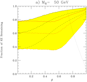
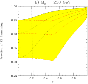
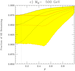
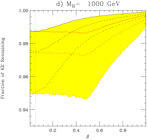
Figure 3: Fraction of the kinetic energy remaining when the $R$-hadron enters the muon detector. The black lines are for the triple-pomeron form of the $R$-hadron nucleon cross section, the red lines are for the simple cut-off form [6]. The interaction length $\lambda_{R}$ is varied between twice the central value (solid), the central value (dashed) and half this value (dot-dashed). The dotted line shows where the $R$-hadron no longer passes the $p_{T}$ cut for the charged $R$-hadron analysis.

Figure 4: Effect of the modelling of the interaction with the detector on the reconstructed $R$-hadron mass for different gluino masses. We show curves for $\lambda_{R}/2$ with the pomeron cross section form (solid), $\lambda_{R}/2$ with the cut-off form (dashed), $\lambda_{R}$ with the pomeron form (dot-dashed) and $2\lambda_{R}$ with the pomeron form (dotted). The probability for producing the $R_{g}^{0}$ is set to zero. We simulate one million events, which is less than one year of high-luminosity running for the all the masses shown.

The percentages of the different species of $R$-hadron is shown in Table 2 for two different gluino masses. We see that the $R_{q\bar{q}}$ hadrons containing only light quarks are predominantly produced with a preference for up and down quarks over strange quarks. The production rates for $R$-hadrons containing a heavy bottom or charm quark is very low. The reason for this is that in our simulation these mesons can only be produced if a gluon that is colour-connected to the gluino perturbatively branches into a heavy-quark pair. This might be an underestimate of the production rate for these states; in the same way, HERWIG tends to underestimate the production rates for bottom and charmonium, which are produced by the same mechanism, at LEP energies. However, given the very low rates it is unlikely that there will be enough events to detect a signal based on displaced vertices due to the decay of the companion heavy quark. The information that could be extracted from these decay signatures would of course be highly interesting.

While all these assumptions are necessary to perform the simulations, they do not have a major effect on the signals we will consider: the phenomenology is mainly determined by the gluino mass and the probability $P_{R_{g}}$ of producing the $R^{0}_{g}$ rather than an $R$-meson in the cluster decays.

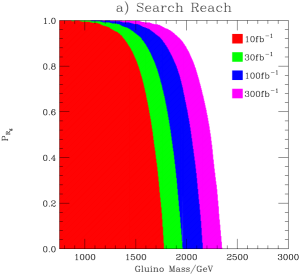
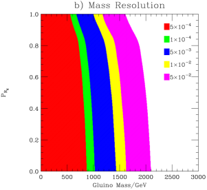
Figure 5: Discovery reach (a) and mass resolution (b) for charged $R$-hadrons. We require the observation of ten charged $R$-hadrons for four different integrated luminosities. We show the mass resolution $\Delta M/M$ for $100{\rm\,fb}^{-1}$.

Variable	Allowed values
$\not\!\!E_{T}\,[{\rm\,GeV}]$	100	150	200	300	400	600	800	1000	1500	2000
$P_{T_{j_{1}}}\,[{\rm\,GeV}]$	100	150	200	300	400	600	800	1000	1500	2000
$P_{T_{j_{2}}}\,[{\rm\,GeV}]$	50	100	150	200	300	400	500	600	800	1000
$\sum P_{T_{j}}\,[{\rm\,GeV}]$	100	200	300	400	500	600	800	1000	1500	2000
$N_{\rm jet}$	2	3	4	5	6	7	8	9	10	11
$S_{T}$	0	0.1	0.2	0.3	0.4	0.5	0.6	0.7	0.8	0.9
$\Delta\phi_{j_{1}}$	0	0.3	0.6	0.9	1.2	1.5	1.8	2.1	2.4	2.7

Table 4: Allowed values for each of the cuts described in the text. In each case the variable is required to be larger than the value quoted.

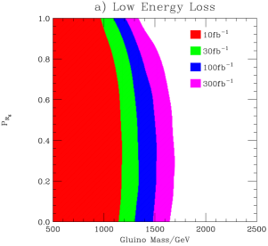
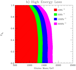
Figure 6: Discovery reach for the missing transverse energy plus jets signal. (a) shows the discovery potential using twice the interaction length and the triple-pomeron form of the cross section, which leads to the smallest energy loss by the $R$-hadron. (b) shows the search reach using half the $R$-hadron interaction length and the cut-off form of the cross section, which leads to the largest energy loss by the $R$-hadron.

In addition to the hadronization, we need to consider the interactions of the $R$-hadrons in the detector. For the interactions of the other particles we use the AcerDet fast simulation [28]. The interaction of the gluino is modelled in the same way as in Ref. [6]. The energy and angular dependence of the $R$-hadron nucleon cross section are modelled using either the cut-off form with a cut-off value of $1{\rm\,GeV}$ or the triple-pomeron form considered in Section IIIA of Ref. [6]. Rather than the approach taken in Ref. [6], which uses the average energy loss in these collisions combined with the depth of the detector in terms of radiation lengths, we propagated the $R$-hadrons through the detector. We generate the distance to the next interaction according to the exponential distribution using the interaction length. The differential cross section is used to calculate the energy loss and change in direction of the $R$-hadron due to the collision. This gives us fluctuations in the energy loss on an event-by-event basis. For the basic properties of the detector we use the parameters given in Table 3, which are based on the ATLAS detector [29]. The energy loss in the electromagnetic and hadronic calorimeters is added to the cells of the calorimeter of the fast detector simulation. For charged $R$-hadrons, which will be detected in the muon chambers, we assume that the momentum measurement will be dominated by the momentum when the $R$-hadron reaches the muon chamber. The time of arrival of this meson at the muon chamber is smeared with a Gaussian of width $0.7\,\rm{ns}$ [23] and the momentum as described in Ref. [23].

Our signatures depend on the energy lost by the $R$-hadron in the detector. The simple cut-off ansatz for the cross section gives too much energy loss for incident pions, whereas the triple-pomeron form gives a good approximation for pion energies lower than $100{\rm\,GeV}$ and too little energy loss at higher energies [6]. We investigate the uncertainty in the modelling of the interaction of the $R$-hadron with the detector in two ways. The simplest approach is to use the two different models of the cross section. The second is to vary also the interaction length $\lambda_{R}$ of the $R$-hadron in the detector between half and twice the value used in Ref. [6]: $\lambda_{R}\sim 16/9\lambda_{\pi}$. The effects of these variations are shown in Fig. 3. We find that the size of the variation decreases as the $R$-hadron mass increases and the effect becomes negligible for the masses we are interested in.

3.3.1 Charged $R$-hadron searches

We consider two main strategies for the analysis. The first closely follows the analysis in Ref. [23] and requires the presence of a charged $R$-hadron, which is reconstructed as a muon. The transverse momentum of the hadron has to be larger than $50{\rm\,GeV}$ (which is sufficient to trigger the event) and the time delay with respect to an ultra-relativistic particle $\Delta t$ has to satisfy $10\;{\rm ns}<\Delta t<50\;{\rm ns}$. An efficiency of 85% is applied for the probability of reconstructing a muon [23].

The mass of the $R$-hadron can then be reconstructed using

$$m^{2}=\frac{p_{D}\Delta t}{x}\left(2p+\frac{p_{D}\Delta t}{x}\right),$$ (9)

where $p$, $p_{D}$ and $x$ are the momentum, the transverse momentum and radius of the muon detectors or the momentum along the beam direction and half-length of the muon detector, depending on whether the $R$-hadron hits the barrel or end-cap detectors.

It is important to check what the effect of the modelling of the $R$-hadron interaction with the calorimeter on the mass determination is. The reconstructed mass is shown for different gluino masses and choices of the interaction with the calorimeter in Fig. 4. As we expect from Fig. 3 the effects of the different choices of the $R$-hadron interaction length and cross section are more apparent at low gluino masses. For all masses, halving the interaction length and using the cut-off form of the cross section leads to more energy loss by the $R$-hadron and hence a lower peak value for the mass and fewer events passing the cuts. For a gluino mass of $50{\rm\,GeV}$, the shift in the average mass is $2.3{\rm\,GeV}$, for a mass of $500{\rm\,GeV}$ the shift is $5{\rm\,GeV}$, and for a mass of $2\,{\rm\,TeV}$ is $6.7{\rm\,GeV}$. In a more realistic study this shift could be corrected for by including the energy deposited in the calorimeter when measuring the $R$-hadron mass.

The cuts we apply should eliminate the Standard Model background [23]. In order to calculate the discovery reach for charged $R$-hadrons we require the observation of ten $R$-hadrons. The results shown in Fig. 3 are using half the default $R$-hadron interaction length and cut-off form of the $R$-hadron interaction cross section. This is the model that gives the highest energy loss. However, the results are not particularly sensitive to this choice and the choice of parameters with the lowest energy loss we consider gives only marginally better results. The reach for this signal is shown in Fig. 5 in the $m_{\tilde{g}}$–$P_{R_{g}}$ plane. We see that the discovery reach extends to over $1.5\,{\rm\,TeV}$ for one year’s running at low luminosity and to over $2\,{\rm\,TeV}$ for one year at high luminosity, apart from a region with low probability of producing a mesonic $R$-hadron.

The resolution of the reconstructed $R$-hadron mass is shown in Fig. 5 for an integrated luminosity of $100{\rm\,fb}^{-1}$. For masses of less than $500{\rm\,GeV}$ the mass can be measured with a precision of better than $0.05\%$. For these masses, this precision is better than the shift in the measured mass due to the energy loss of the charged $R$-hadron in the calorimeter. For higher masses the resolution decreases, but it is still better than $1\%$ for masses up to $1.5\,{\rm\,TeV}$. This is an effect of the mass shift due to the energy loss in the calorimeter.

3.3.2 Neutral $R$-hadron searches

A second signal that does not depend on the production of charged $R$-hadrons is the classic jets plus missing transverse energy signature. Neutral $R$-hadrons will of course always be produced, even if no $R^{0}_{g}$ hadrons are created, because the $R_{\rho}^{0}$ will be produced with the same probability as the charged $R$-hadrons, see Table 2. For neutral $R$ hadrons only there will be no production of charged leptons in association with the gluino signal, apart from the decays of heavy hadrons. On the other hand, there will be fake muons from the charged $R$-hadrons. In analysing the missing transverse energy signal we therefore require that there be no leptons in the signal, so as to reduce the background from Standard Model $W$ and $Z$ production. When applying this cut we assume that charged $R$-hadrons that pass the same isolation cut as muons will be reconstructed as muons. This is a conservative assumption, because some of them will not be reconstructed, because of the large time delay.

Our approach for neutral $R$-hadrons is close to that in Ref. [30]. The Standard Model QCD, top quark, $W$+jets and $Z$+jets signals are simulated using HERWIG6.5 [25] in logarithmic transverse momentum bins in order to increase the number of events simulated at high-$p_{T}$, which are most likely to contribute to the background. A number of variables are used to distinguish between the signal and background events:
(1) the missing transverse energy $\not\!\!E_{T}$;
(2) the transverse momentum of the hardest jet $P_{T_{j_{1}}}$;
(3) the transverse momentum of the second hardest jet $P_{T_{j_{2}}}$;
(4) the scalar sum of the transverse momentum of the jets in the event $\sum P_{T_{j}}$;
(5) the number of jets $N_{\rm jet}$;
(6) the transverse sphericity of the event $S_{T}$; see e.g. Ref. [1] for the definition of $S_{T}$;
(7) the difference in azimuthal angle between the direction of the hardest jet and $\not\!\!E_{T}$.

We test different sets of cuts on these variables to maximize the statistical significance of the signal on a point-by-point basis. The values of the cuts are given in Table 4. The lowest value of the cuts on the missing transverse momentum and on the transverse momentum of the first jet are sufficient for the event to be triggered [30]. We define the significance as $S/\sqrt{S+B}$, to minimize the effect of statistical fluctuations in the signal and background samples and require a $5\sigma$ significance.

The discovery potential for this signal is shown in Fig. 6 for the largest and smallest energy loss by the $R$-hadron considered in our modelling of the $R$-hadron interaction with the detector. For both choices of this interaction, the discovery potential is smallest for high probabilities of producing the $R_{g}^{0}$, and it increases with the probability of producing an $R$-meson. This is because there can be significant missing transverse energy when a neutral $R$-hadron is produced together with a charged one. If the charged $R$-hadron is considered to be a jet with a non-isolated muon, this gives a jet and significant missing transverse energy. This also explains why the model of the interaction with less energy loss gives a lower signal: if the charged $R$-hadrons deposit less energy in the calorimeter, they are more likely to be considered as leptons and not included in the analysis, which reduces the signal.

Even using this model of low interaction with the detector, gluinos with masses up to $1.1\,{\rm\,TeV}$ can be discovered with $100\,\rm{fb}^{-1}$ integrated luminosity, and gluinos with masses up to $1.3\,{\rm\,TeV}$ can be observed with an integrated luminosity of $300\,\rm{fb}^{-1}$. The main difference between the searches for charged and neutral $R$-hadrons is that in the missing transverse energy search we will not be able to measure the gluino mass except through the total cross section. However, this might be possible for gluino masses of ${\cal O}({\rm\,TeV})$, if we look for gluino–gluino bound states leading to a peak in the two-jet invariant mass spectrum [32].

Figure 7: Cross sections for chargino and neutralino pair production in $e^{+}e^{-}$ collisions [38], assuming the reference point in eq.(2).

4 Yukawa couplings from gaugino–Higgsino mixing

If split supersymmetry should be realized in nature, the observation of the gluino, charginos and neutralinos will only be the first task. Once these states are discovered, we will have to show that they constitute a weak-scale SUSY Lagrangian. At the LHC, the immediate challenge will be the determination of the quantum numbers of the new particles [33]. Even if we take for granted their fermionic nature, this does not establish them as SUSY partners: the set of colour-octet, weak isosinglet, isotriplet, and a pair of isodoublet fermions (as present in the MSSM) makes up a minimal non-trivial extension of the Standard Model that is anomaly-free and consistent with gauge coupling unification. A quantitative hint for supersymmetry is given by the off-diagonal elements in the mass matrices. They determine the mixing of gauginos and higgsinos into charginos and neutralinos as mass eigenstates. This mixing is possible because supersymmetry transformations maintain Standard Model quantum numbers. These off-diagonal entries in the mass matrix also constitute the neutralino and chargino Yukawa couplings. In SpS, these off-diagonal entries follow, up to renormalization group effects, the predicted MSSM pattern.

Without any mixing, the only production channels (in the absence of scalars) in $\bar{q}q$ or $e^{+}e^{-}$ annihilation are $\tilde{\chi}^{+}_{1}\tilde{\chi}^{-}_{1}$, $\tilde{\chi}^{+}_{2}\tilde{\chi}^{-}_{2}$, $\tilde{\chi}^{\pm}_{1}\tilde{\chi}^{0}_{2}$, $\tilde{\chi}^{\pm}_{2}\tilde{\chi}^{0}_{3,4}$, and $\tilde{\chi}^{0}_{3}\tilde{\chi}^{0}_{4}$. Moreover, all these produced particles would be stable. Any other production or decay channel requires either a finite coupling to $s$ channel gauge bosons through mixing or the presence of scalars. The observation of additional production channels and the measurement of decay branching ratios is therefore an indirect probe of the neutralino and chargino Yukawa couplings. The usual analysis of gauge couplings and the corresponding gaugino-sfermion-fermion couplings will fail in SpS scenarios, because the squarks are much heavier than the gauginos [34]. To measure the neutralino and chargino mixing matrices, a precise mass measurement is sufficient. Without gaugino–Higgsino mixing the mass matrices are determined by the MSSM parameters $M_{1},M_{2}$ and $\mu$. The gaugino–Higgsino mixing adds terms of the order of $M_{Z}$ and introduces the additional parameter $\tan\beta$, leading to four MSSM parameters altogether. As shown before [35], these parameters can be extracted from the six neutralino and chargino masses by using a simple fit, properly including experimental errors [36].

Figure 7 displays the cross sections for chargino and neutralino pair production in $e^{+}e^{-}$ collisions for the point of eq.(2) as a function of the collider energy. With one exception, all channels have cross sections larger than $0.1{\rm\,fb}$ and the threshold value for $\tilde{\chi}^{+}_{1}\tilde{\chi}^{-}_{1}$ production is as large as $1\;{\rm\,pb}$. A linear collider with moderate energy and high luminosity would be optimal to probe all these processes, and some kind of fit is the proper method to extract the weak-scale Lagrangean parameters. We emphasize that these cross sections [37] as well as the masses [16] are known to NLO. However, because we are mainly interested in the error on the extracted underlying parameters and less interested in their central values, we limit our fit to leading order observables.

Previous studies of the chargino and neutralino systems concentrated on the extraction of the mass parameters $M_{1},M_{2},\mu$, while the off-diagonal elements were fixed or at least related to each other by the MSSM relations. In SpS, the four off-diagonal entries in the mass matrices are independent observables. As defined in eq.(4) we parametrize the couplings $\tilde{g}_{u,d}^{(\prime)}$, introducing an additional factor $(1+\kappa_{u,d}^{(\prime)})$ with respect to the MSSM values [8]. While these $\kappa$ parameters vanish to leading order in the complete weak-scale MSSM, the SpS renormalization flow between the matching scale $\widetilde{m}$ and the electroweak scale induces non-zero values of order $\kappa^{(\prime)}_{i}=-0.2\ldots 0.2$. If we are able to detect deviations of this size at a collider, we can both establish the supersymmetric nature of the model and verify the matching condition to the MSSM at $\widetilde{m}$.

Figure 8: Fit to 10000 sets of mass and cross section pseudo-measurements at a future linear collider (upper) and at the LHC (lower). The fitted parameters include only $\kappa_{u}$ with a central value zero. At the LHC $\tan\beta=4$ is fixed.

As mentioned above, the neutralino and chargino mixing matrices can be measured at a future linear collider, in continuum production as well as through a threshold scan [39]. The six masses alone are sufficient to determine all the usual MSSM parameters $M_{1},M_{2},\mu,\tan\beta$, plus one additional $\kappa$. Because the predicted values $\kappa^{(\prime)}_{i}$ are small, the correct treatment of the experimental accuracies is crucial. For our central parameter point of eq.(2) we compute the masses and the cross sections shown in Fig. 7, with the exception of the $\tilde{\chi}^{0}_{1}\tilde{\chi}^{0}_{1}$ channel. To all observables we assign an experimental error, which in our simplified treatment is a relative error of $0.5\%$ on all linear-collider mass measurements [39], $5\%$ on all LHC mass measurements [40], and the statistical uncertainty on the number of events at a linear collider corresponding to $100{\rm\,fb}^{-1}$ of data at a $1{\rm\,TeV}$ collider after all efficiencies. The assumption that the LHC might be able to see all six gauginos and Higgsinos and measure all their masses is very optimistic, so we will only use it to derive the maximum sensitivity the LHC could achieve.

Moreover, the precision of the theoretical cross section prediction [17] and the precision of the measurement of cross sections and branching ratios at the LHC is likely to be insufficient to allow the extraction of small mixing parameters. Around the central parameter point we randomly generate 10000 sets of pseudo-measurements, using a Gaussian smearing. Out of each of these sets we extract the MSSM parameters. In principle, we could simply invert the relation between the masses and the Lagrangian parameters analytically. However, after smearing, this inversion will not have a unique and well-defined solution; therefore we use a fit to solve the overconstrained system. The distribution of the 10000 fitted values should return the right central value and the correctly propagated experimental error on the parameter determination. If necessary, we apply another maximum $\chi^{2}$ cut on the 10000 fits, to get rid of secondary minima. The distributions of the measurements are not necessarily Gaussian, and there might be non-trivial correlations between different measurements. At the end, the crucial questions are: (i) is the error on the parameter measurements sufficient to claim agreement with the MSSM prediction, and (ii) Is the measurement good enough to probe the renormalization group effects of the heavy scalars in SpS?

	Fit $\tan\beta$	$m_{i}$	$\sigma_{ij}$	$\Delta\kappa_{u}$	$\Delta\kappa_{d}$	$\Delta\kappa^{\prime}_{u}$	$\Delta\kappa^{\prime}_{d}$
Tesla		$\bullet$	$\bullet$	$0.9\times 10^{-2}$	$3\times 10^{-2}$	$1.3\times 10^{-2}$	$4\times 10^{-2}$
Tesla	$\bullet$	$\bullet$	$\bullet$	$1.2\times 10^{-2}$	$5\times 10^{-2}$	$2\times 10^{-2}$	$5\times 10^{-2}$
Tesla		$\bullet$		$1.1\times 10^{-2}$	$5\times 10^{-2}$	$3\times 10^{-2}$	$8\times 10^{-2}$
Tesla	$\bullet$	$\bullet$		$1.2\times 10^{-2}$	$11\times 10^{-2}$	$4\times 10^{-2}$	$8\times 10^{-2}$
LHC		$\bullet$		$2.2\times 10^{-1}$	$6\times 10^{-1}$	$2.7\times 10^{-1}$	$8\times 10^{-1}$
Tesla		$\bullet$	$\bullet$	$1.4\times 10^{-2}$	$5\times 10^{-2}$	$3\times 10^{-2}$	$10\times 10^{-2}$
Tesla∗	$\bullet$	$\bullet$	$\bullet$	$1.7\times 10^{-2}$	$9\times 10^{-2}$	$4\times 10^{-2}$	$13\times 10^{-2}$
Tesla	fix $\tan\beta=3$	$\bullet$	$\bullet$	$1.6\times 10^{-2}$	$4\times 10^{-2}$	$4\times 10^{-2}$	$9\times 10^{-2}$
Tesla∗	$\kappa_{i}\neq 0$	$\bullet$	$\bullet$	$1.4\times 10^{-2}$	$5\times 10^{-2}$	$4\times 10^{-2}$	$11\times 10^{-2}$

Table 5: Error on the determination of $\kappa_{i}$ from measured masses and possibly production cross sections. For the first five lines, all but one $\kappa$ are fixed to zero, the fitted $\kappa$ has the central value zero. In the last four lines, all four $\kappa_{i}$ are fitted simultaneously. The very last line assumes the predicted central values of $\kappa_{i}$ in our SpS parameter point. The error on the mass measurements is $0.5\%$ for Tesla and $5\%$ for the LHC. The sets of measurements marked by ^∗ include a maximum $\chi^{2}$ cut to get rid of secondary minima.

As a first test of our approach we set all four non-MSSM contributions to zero ($\kappa^{(\prime)}_{i}=0$) and add one of the four anomalous Yukawa couplings to the set of fitted parameters, keeping the other three fixed during the fit. In Fig. 8 we show the result for a combined fit of $M_{1},M_{2},\mu,\kappa_{u}$ and possibly $\tan\beta$. At a linear collider we can extract the mass parameters at the percentage level and the best measured anomalous coupling, $\kappa_{u}$, to typically $0.01$. In Table 5 we see that the error on the determination of all four $\kappa$ values at a linear collider is a few per cent. Generically, the error on $\kappa^{(\prime)}_{d}$ is larger than the error on $\kappa^{(\prime)}_{u}$, because $\kappa^{(\prime)}_{d}$ is accompanied by $\cos\beta$ while $\kappa^{(\prime)}_{u}$ enters with an additional factor $\sin\beta$. We checked that for large $\tan\beta$ values, e.g. $\tan\beta=30$, only $\kappa^{(\prime)}_{u}$ can be extracted with a reasonable error. If we fix all but one $\kappa$ to their zero MSSM prediction, the remaining off-diagonal entries in the mass matrices are determined by $\tan\beta$. While we might hope to extract $\tan\beta$ from the Higgs sector, we also test the prospects of determining it in our fit. In Table 5 we see that errors only slightly degrade when we include $\tan\beta$ in the set of parameters we fit to, and in Fig. 8 we see that the determination of $\tan\beta$ indeed works very well.

Since we are limiting the number of unknowns to four or five (depending on whether or not we fit $\tan\beta$), the six mass measurements should be sufficient to extract one anomalous Yukawa coupling parameter. Indeed, in Table 5 we see that the precision on the $\kappa^{(\prime)}_{i}$ suffers only slightly when we limit our set of measurements to the masses alone and assume $\tan\beta$ to be known. This is an effect of the overwhelming precision of the mass measurement through threshold scans, our assumed error of $0.5\%$ is even conservative. Adding $\tan\beta$ to the fit shows, however, that with five parameters and six measurements our analyses are starting to lose sensitivity. When we try to extract the Lagrangian parameters from a set of mass measurements at the LHC, the errors on the mass parameters $M_{1},M_{2},\mu$ inflate to the $10\%\ldots 20\%$ level, as shown in Fig. 8. While we might still be able test if the $\kappa^{(\prime)}_{u}$ follow the weak-scale MSSM prediction, the experimental precision is clearly insufficient to test the SpS renormalization group effects. Moreover, it is not clear if all neutralino and chargino masses could be extracted at the LHC, because all current search strategies rely on squark and gluino cascade decays [40]. Last but not least, we do not know if we will be able to measure $\tan\beta$ in the Higgs sector, and including $\tan\beta$ in the LHC fit will make the extraction of $\kappa^{(\prime)}_{u}$ even less promising.

Figure 9: Fit to 10000 sets of mass and cross section pseudo-measurements at a future linear collider. All four $\kappa^{(\prime)}_{i}$ are extracted simultaneously. The central values are set to zero as in the MSSM (upper) and to the example SpS values (lower). The MSSM zero prediction is indicated in the lower line of histograms.

At the linear collider, adding the cross sections as independent measurements allows us to fit all four $\kappa^{(\prime)}_{i}$ simultaneously. This is the proper treatment, unless we would have reasons to believe that some of the $\kappa^{(\prime)}_{i}$ are predicted to be too small to be measured. This means that $\tan\beta$ is no longer an independent parameter: we can fix it in the fit, to reduce the number of unknown Lagrangian parameters. The error on the determination of all four $\kappa^{(\prime)}_{i}$ is shown in Fig. 9, including the error on $M_{2}$, to illustrate that adding all four anomalous couplings to the fit has little impact on the measurement of the dominant Lagrangian mass parameters. In Table 5 the errors for the simultaneous $\kappa$ measurements are compared with the single-$\kappa$ fit. If we fix $\tan\beta$ to the correct value, the error bands increase by a factor of 2.5 at the maximum, when we move to a combined extraction of all $\kappa^{(\prime)}_{i}$. Adding $\tan\beta$ to the fit shows us to which degree we are already limited by the number of useful measurements: the quality of the measurements suffers considerably and we have to avoid secondary minima. However, as we already pointed out, $\tan\beta$ should be fixed if we limit ourselves to independent parameters. The question to know, what happens if we fix it to a wrong value. From eq.(4) we see that assigning a wrong value to $\tan\beta$ should just move the central values of the extracted $\kappa^{(\prime)}_{i}$, in our case away from zero. As an example, for an assumed value $\tan\beta$ the four anomalous coupling measurements are centred around $0.023,-0.23,0.023,-0.23$ instead of zero, in the order of Table 5. Again in Table 5 we see that the effect on the errors is indeed negligible.

The last step left is from the case $\kappa^{(\prime)}_{i}=0$ to the values predicted by SpS, eq.(4). This is merely a cross-check, because the error in the extraction of the anomalous couplings should not significantly depend on their central values. Indeed, in Fig. 9 and in Table 5 we see that the central value has no visible effect on the errors, even though in our case it makes the fit more vulnerable to secondary minima. As usual, we get rid of the secondary minimum using a maximum-$\chi^{2}$ value for the 10000 pseudo-measurements, reducing the number of entries in the histogram by $17\%$. These results for the linear collider indeed indicate that we could not only confirm that the Yukawa couplings and the neutralino and chargino mixing follow the predicted MSSM pattern; for the somewhat larger $\kappa^{\prime}_{i}$ values we can even distinguish the complete weak-scale MSSM from a SpS spectrum.

5 Direct measurement of Yukawa couplings

Figure 10: Signal and background cross sections for associated production of neutralinos and charginos with a Higgs boson in $e^{+}e^{-}$ collisions [38].

While the elements of the neutralino and chargino mixing matrices depend on the Yukawa couplings in a complicated way, the cross sections for chargino/neutralino pair production in association with a Higgs boson are directly proportional to these parameters. Therefore, the observation of $H\tilde{\chi}\tilde{\chi}$ final states [38, 42] could add to our knowledge of the Yukawa couplings that can be gained in chargino/neutralino pair production.

If decays of the kind $\chi^{\pm}_{2}\to\chi^{\pm}_{1}H$ or $\chi^{0}_{j}\to\chi^{0}_{i}H$ proceed with a significant rate, these branching fractions are determined by the Yukawa couplings in conjunction with the mixing effects and should be included in a global fit. Unfortunately, for low values of the mass parameters $M_{1},M_{2},\mu$ this is less likely to happen than in the MSSM, since the Higgs is considerably heavier, so that some channels are no longer kinematically accessible. In particular, for the reference point eq.(2), no such decay is possible.

However, in this situation there is still associated production of charginos and neutralinos with a Higgs boson in the continuum, which can in principle be observed at a high-luminosity $e^{+}e^{-}$ collider. Figure 10 displays the cross sections as a function of the collider energy. Like all $s$-channel processes, the curves peak immediately above the respective threshold energies. The dominant Standard Model background to these processes consists of Higgs production in association with $Z$ and $W$ bosons and a neutrino pair, also shown in Fig. 10. The neutrino pair can either originate from a $Z$ boson or from the continuum ($W$-fusion processes), where in the latter case the total cross section increases with energy. Last but not least, we have to take into account processes with a forward-going electron in the final state, which may escape undetected.

Although the backgrounds are substantial, they do not affect all signals simultaneously, and they can be reduced significantly by kinematical cuts. Assuming thus that processes with Higgs-strahlung off a chargino or neutralino can be identified above the background, they will depend on the $\kappa$ directly and through the neutralino and chargino masses. Apparently, the neutralino processes have a rate too small to help in disentangling the parameters. However, in contrast to chargino pair production, $\tilde{\chi}^{+}\tilde{\chi}^{-}H$ associated production depends on $\kappa_{u}$ and is independent of $\kappa^{\prime}_{u}$, so its inclusion in a global fit reduces the correlation between these two parameters. Because the dependence of the cross sections on $\kappa^{\prime}_{d}$ is fairly weak, this parameter will pose a challenge for the direct extraction.

The precision that can be achieved from cross section measurements is given by the statistical error on the cross section. Assuming $1{\rm\,ab}^{-1}$ of integrated luminosity, we could collect a sample of at maximum 200 (100) signal events, which gives us an error of $7\%(10\%)$ on the cross section measurement and therefore an error of $3.5\%(5\%)$ on the measurement of the Yukawa coupling. This number could be competitive with our estimates for the indirect measurement shown in Table 5. However, even if we can extract the masses involved using a threshold scan, the extraction of couplings from cross sections is always plagued by theoretical uncertainties due to higher orders and systematical experimental uncertainties. More detailed studies are required to obtain a final verdict on the errors [41].

6 Conclusions

Recently, models of split supersymmetry have been suggested. If we are willing to accept a high degree of fine-tuning for the separation between the weak scale and the Planck scale, decoupling of all sfermions can solve problems which usual supersymmetry has in the flavour sector, mediating proton decay or leading to large electric dipole moments. In particular, gauge-coupling unification and the existence of a dark matter candidate naturally survive the decoupling of the scalar partner states.

For collider experiments this means that only gauginos and Higgsinos are light enough to be produced, because their masses can be protected by a chiral symmetry. At the LHC we will observe a long-lived gluino. Over almost the entire parameter space, we will be able to see the resulting charged $R$-hadrons for gluino masses larger than $2{\rm\,TeV}$ and determine the gluino mass to better than $1\%$. In the region where the probability of producing a mesonic $R$-hadron is small, the reach can be enhanced by the classic jets plus missing energy channel. In the case of neutral $R$-hadrons this leaves us with a reach of between $1.3{\rm\,TeV}$ and $1.8{\rm\,TeV}$ for the gluino mass, depending on the details of the $R$-hadron spectroscopy. Because we cover neutral as well as charged $R$-hadrons our result is independent of the mass hierarchy of the $R$-hadrons and the possible $R$-hadron decays into each other. We emphasize that the interaction of the gluino in the detector is currently being studied in more detail and we expect improved estimates for the discovery reach as well as for the mass measurement [31].

Because cascade decays of squarks and gluinos leading to subsequent neutralino and chargino signals will not be available for split supersymmetry models, we give the direct production cross sections for all possible channels. It will be a challenge to extract these signals from the Standard Model backgrounds and separate them to gain access to some of the model parameters.

Obviously, a future high-luminosity linear collider will be perfectly suited for this kind of precision measurements. Integrating out the scalars at a high scale leads to renormalization group effects for the neutralino and chargino Yukawa couplings and their mixing matrices. At a linear collider we will be able to see all neutralinos and charginos and measure their masses and cross sections, provided the collider energy is sufficient. From these measurements we can extract the mixing matrix elements (with contributions from the anomalous Yukawa couplings) to better than $10\%$ accuracy. The estimate of the experimental errors is based on a similar parameter point studied in Ref. [39]. For a final statement about the possible accuracy with which we can extract the anomalous Yukawa couplings one would have to combine a detector simulation with the proper treatment of the theoretical errors, which is beyond the scope of this paper. Through the associated production of charginos with a Higgs we might also have direct access to these Yukawa couplings. If split supersymmetry effects are large enough we will be able not only to confirm that neutralinos and charginos are indeed the partners of gauge bosons and Higgs bosons — we will also gain insight into the heavy decoupled spectrum.

Acknowledgements

First, we would like to thank Andrea Romanino for his great help cross-checking our results with Ref. [8]. Moreover, we would like to thank Jürgen Reuter for providing the MSSM code for the WHIZARD/O’Mega package and for reading the manuscript. We would like to thank Aafke Kraan, Tim Jones, Peter Zerwas, Bryan Webber and Andy Parker for fruitful discussions, which had a major impact on many aspects of this work. Finally, we would like to thank Tim Jones for carefully reading this manuscript. E.S and T.P. are grateful to the DESY theory group for their kind hospitality.

References

- [1] ATLAS Collaboration, TDR, vol. 2, CERN-LHCC/99-015 (1999); CMS Collaboration, CERN-LHCC/94-38 (1994).
- [2] L. Alvarez-Gaumé, J. Polchinski and M. B. Wise, Nucl. Phys. B 221, 495 (1983); L. E. Ibañez, Phys. Lett. B 118, 73 (1982); J. R. Ellis, D. V. Nanopoulos and K. Tamvakis, Phys. Lett. B 121, 123 (1983); K. Inoue, A. Kakuto, H. Komatsu and S. Takeshita, Prog. Theor. Phys. 68, 927 (1982) [Erratum-ibid. 70, 330 (1983)]; A. H. Chamseddine, R. Arnowitt and P. Nath, Phys. Rev. Lett. 49, 970 (1982).
- [3] M. Dine, W. Fischler and M. Srednicki, Nucl. Phys. B 189, 575 (1981); S. Dimopoulos and S. Raby, Nucl. Phys. B 192, 353 (1981); C. R. Nappi and B. A. Ovrut, Phys. Lett. B 113, 175 (1982); L. Alvarez-Gaumé, M. Claudson and M. B. Wise, Nucl. Phys. B 207, 96 (1982); M. Dine and A. E. Nelson, Phys. Rev. D 48, 1277 (1993); M. Dine, A. E. Nelson and Y. Shirman, Phys. Rev. D 51, 1362 (1995); M. Dine, A. E. Nelson, Y. Nir and Y. Shirman, Phys. Rev. D 53, 2658 (1996).
- [4] For an overview, see e.g. M. Drees and S. P. Martin, arXiv:hep-ph/9504324.
- [5] G. R. Farrar and P. Fayet, Phys. Lett. B 76, 575 (1978).
- [6] H. Baer, K. M. Cheung and J. F. Gunion, Phys. Rev. D 59, 075002 (1999).
- [7] N. Arkani-Hamed and S. Dimopoulos, arXiv:hep-th/0405159.
- [8] G. F. Giudice and A. Romanino, arXiv:hep-ph/0406088.
- [9] S. Weinberg, Phys. Rev. Lett. 59, 2607 (1987).
- [10] L. Susskind, arXiv:hep-th/0405189.
- [11] S. Dawson and H. Georgi, Phys. Rev. Lett. 43, 821 (1979); M. B. Einhorn and D. R. T. Jones, Nucl. Phys. B 196, 475 (1982).
- [12] A. Arvanitaki, C. Davis, P. W. Graham and J. G. Wacker, arXiv:hep-ph/0406034.
- [13] A. Pierce, arXiv:hep-ph/0406144; J. R. Ellis, T. Falk, G. Ganis, K. A. Olive and M. Schmitt, Phys. Rev. D 58, 095002 (1998); For a recent review, see e.g. G. Bertone, D. Hooper and J. Silk, arXiv:hep-ph/0404175.
- [14] P. M. Ferreira, I. Jack and D. R. T. Jones, Phys. Lett. B 387, 80 (1996); http://www.liv.ac.uk/dij/betas
- [15] For a recent review, see e.g. S. Heinemeyer, arXiv:hep-ph/0407244; R. Mahbubani, arXiv:hep-ph/0408096.
- [16] T. Fritzsche and W. Hollik, Eur. Phys. J. C 24, 619 (2002); W. Oller, H. Eberl, W. Majerotto and C. Weber, Eur. Phys. J. C 29, 563 (2003).
- [17] W. Beenakker, R. Höpker, M. Spira and P. M. Zerwas, Nucl. Phys. B 492, 51 (1997); W. Beenakker, M. Klasen, M. Krämer, T. Plehn, M. Spira and P. M. Zerwas, Phys. Rev. Lett. 83, 3780 (1999); Prospino2.0, http://pheno.physics.wisc.edu/plehn
- [18] M. Mühlleitner, A. Djouadi and Y. Mambrini, arXiv:hep-ph/0311167.
- [19] M. S. Chanowitz and S. R. Sharpe, Phys. Lett. B 126, 225 (1983).
- [20] M. Foster and C. Michael [UKQCD Collaboration], Phys. Rev. D 59, 094509 (1999).
- [21] For a review, see e.g. M. Neubert, Phys. Rept. 245, 259 (1994); M. Neubert, arXiv:hep-ph/0001334.
- [22] F. Buccella, G. R. Farrar and A. Pugliese, Phys. Lett. B 153, 311 (1985).
- [23] B. C. Allanach, C. M. Harris, M. A. Parker, P. Richardson and B. R. Webber, JHEP 0108, 051 (2001).
- [24] I. Hinchliffe and F. E. Paige, Phys. Rev. D 60, 095002 (1999); G. Polesello and A. Rimoldi, ATL-MUON-99-006.
- [25] G. Corcella et al., JHEP 0101, 010 (2001); G. Corcella et al., arXiv:hep-ph/0210213.
- [26] B. R. Webber, Nucl. Phys. B 238, 492 (1984).
- [27] G. Karl and J. Paton, Phys. Rev. D 60, 034015 (1999).
- [28] E. Richter-Was, arXiv:hep-ph/0207355.
- [29] ATLAS Collaboration, TDR, vol. 1, CERN-LHCC/99-014.
- [30] A. J. Barr, C. G. Lester, M. A. Parker, B. C. Allanach and P. Richardson, JHEP 0303, 045 (2003).
- [31] A. C. Kraan, arXiv:hep-ex/0404001.
- [32] J. H. Kühn and S. Ono, Phys. Lett. B 142, 436 (1984); T. Goldman and H. Haber, Physica 15D, 181 (1985); E. Chikovani, V. Kartvelishvili, R. Shanidze and G. Shaw, Phys. Rev. D 53, 6653 (1996).
- [33] A. J. Barr, arXiv:hep-ph/0405052.
- [34] H. C. Cheng, J. L. Feng and N. Polonsky, Phys. Rev. D 57, 152 (1998).
- [35] J. L. Feng, M. E. Peskin, H. Murayama and X. Tata, Phys. Rev. D 52, 1418 (1995); S. Y. Choi, A. Djouadi, M. Guchait, J. Kalinowski, H. S. Song and P. M. Zerwas, Eur. Phys. J. C 14, 535 (2000); S. Y. Choi, J. Kalinowski, G. Moortgat-Pick and P. M. Zerwas, Eur. Phys. J. C 22, 563 (2001) [Addendum-ibid. C 23, 769 (2002)]; S. H. Zhu, arXiv:hep-ph/0407072.
- [36] V. D. Barger, T. Han, T. J. Li and T. Plehn, Phys. Lett. B 475, 342 (2000); V. D. Barger, T. Falk, T. Han, J. Jiang, T. Li and T. Plehn, Phys. Rev. D 64, 056007 (2001).
- [37] W. Oller, H. Eberl and W. Majerotto, Phys. Lett. B 590, 273 (2004); T. Fritzsche and W. Hollik, arXiv:hep-ph/0407095.
- [38] W. Kilian, LC-TOOL-2001-039; W. Kilian, Proc. ICHEP 2002, Amsterdam; M. Moretti, T. Ohl and J. Reuter, arXiv:hep-ph/0102195; http://www-ttp.physik.uni-karlsruhe.de/whizard
- [39] J. A. Aguilar-Saavedra et al. [ECFA/DESY LC Physics Working Group Collaboration], arXiv:hep-ph/0106315; B. C. Allanach, G. A. Blair, S. Kraml, H. U. Martyn, G. Polesello, W. Porod and P. M. Zerwas, arXiv:hep-ph/0403133.
- [40] H. Bachacou, I. Hinchliffe and F. E. Paige, Phys. Rev. D 62, 015009 (2000); B. C. Allanach, C. G. Lester, M. A. Parker and B. R. Webber, JHEP 0009, 004 (2000).
- [41] R. Lafaye, T. Plehn and D. Zerwas, arXiv:hep-ph/0404282; http://sfitter.web.cern.ch; see also http://www-flc.desy.de/fittino
- [42] G. Ferrera and B. Mele, arXiv:hep-ph/0407108.