P-P Total Cross Sections at VHE from Accelerator Data

J. Pérez-Peraza, A. Sánchez-Hertz, M. Alvarez-Madrigal

Instituto de Geofísica, UNAM, Coyoacán, México D.F., MEXICO

J. Velasco, A. Faus-Golfe

IFIC – Instituto de Física Corpuscular
Centro Mixto CSIC–Universitat de València, Spain
A. Gallegos-Cruz

Ciencias Básicas, UPIICSA, I.P.N., Iztacalco, Mexico D.F, MEXICO

Up today estimations of proton-proton total cross sections, $\sigma_{tot}^{pp}$, at very high energies are obtained from cosmic rays ($>10^{17}$ eV) by means of some approximations and the knowledge of the measured proton-air cross section at these energies. Besides, $\sigma_{tot}^{pp}$ are measured with present day high energy colliders up to nearly $2$ TeV in the center of mass ($\sim\ 10^{15}$ eV in the laboratory). Several theoretical, empirical or semi-empirical parameterizations, very successful for interpolation at accelerator energies, can then be used to extrapolate the measured value to cosmic ray energies and get a reasonable estimation of cross sections at higher energies ($\sim\ 10^{17}$ eV). When both cross section estimations - from accelerators and cosmic rays - are compared, a disagreement is observed, amounting to more than $10\%$, showing a discrepancy beyond statistical errors. Here we use a phenomenological model based on the Multiple-Diffraction approach to successfully describe data at accelerator energies. Then we estimate with this model $\sigma_{tot}^{pp}$ at cosmic ray energies. The employed fitting method associates the model free-parameters to the data of only two physical observable: the differential cross-section and the parameter $\rho$. The model predictions for estimations of $\sigma_{tot}^{pp}$ are then compared with data of total cross-sections. On the basis of regression analysis we determine confident error bands, analyzing the sensitivity of our predictions to the employed data for extrapolation. : using data at 546 and 1.8 TeV, our extrapolations for $\sigma_{tot}^{pp}$ are only compatible with the Akeno cosmic ray data, predicting a slower rise with energy than other cosmic ray results and other extrapolation methods. We discuss our results within the context of constraints in the light of future accelerator and cosmic ray experimental results.

INTRODUCTION

Recently a number of difficulties in uniting accelerator and cosmic ray values of proton-proton, $\sigma_{tot}^{pp}$, and antiproton-proton, $\sigma_{tot}^{\bar{p}p}$, hadronic total cross-sections, within the frame of the highest up-to-date data have been summarized [1]. Such united picture appears to be of the highest importance for the interpretation of results of new cosmic ray experiments as the HiRes [2] and in designing proposals that are currently in progress as the Auger Observatory [3], as well as in designing detectors for future accelerators, as the CERN pp Large Hadron Collider (LHC) [4]. Although most of accelerator measurements of $\sigma_{tot}^{pp}$ and $\sigma_{tot}^{\bar{p}p}$ at center of mass energies $\sqrt{s}\leq$ 1.8 TeV are quite consistent among them, this is unfortunately not the case for cosmic ray experiments at $\sqrt{s}>6$ TeV where some disagreements exist among different experiments. This is also the case among different predictions from the extrapolation of accelerator data up to cosmic ray energies: whereas some works predict smaller values of $\sigma_{tot}^{pp}$ than those of cosmic ray experiments (e.g. [5, 6]) other predictions agree at some specific energies with cosmic ray results (e.g. [7]). Dispersion of cosmic ray results are mainly associated to the strong model-dependence of the relation between the basic hadron-hadron cross-section and the hadronic cross-section in air. The later determines the attenuation length of hadrons in the atmosphere, which is usually measured in different ways, and depends strongly on the rate ($k$) of energy dissipation of the primary proton into the electromagnetic shower observed in the experiment: such a cascade is simulated by different Monte Carlo technics implying additional discrepancies between different experiments. Furthermore, $\sigma_{tot}^{pp}$ in cosmic ray experiments is determined from $\sigma_{p-air}^{inel}$ using a nucleon-nucleon scattering amplitude which is frequently in disagreement with most of accelerator data [1].

On the other hand, we dispose of many parameterizations (purely theoretically, empirical or semi-empirical based) that fit pretty well the accelerator data. Most of them agree that at the energy of the future LHC (14 TeV in the center of mass) or higher the rise in energy of $\sigma_{tot}^{pp}$ will continue, though the predicted values differ from model to model. We claim that both the cosmic ray and parametrization approaches must complement each other in order to draw the best description of the proton-proton hadronic cross-section behavior at ultra high energies. However, the present status is that due to the fact that interpolation of accelerator data is nicely obtained with most of parametrization models, it is expected that their extrapolation to higher energies be highly confident: as a matter of fact, parameterizations are usually based in a short number of fundamental parameters, in contrast with the difficulties found in deriving $\sigma_{tot}^{pp}$ from cosmic ray results [1]. With the aim of contributing to the understanding of this problem, in this paper we first briefly analyze in the first two sections the way estimations are done for $\sigma_{tot}^{pp}$ from accelerators as well as from cosmic rays. We find serious discrepancies among both estimations. In section III we describe the Multiple Diffraction model and the employed method to evaluate the model parameters on basis of data of only two physical observable: the differential cross-section and the parameter $\rho$. For the goal of the present approach we neglect crossing symmetry. In the fourth section we present a suitable parametrization to high energies of the free energy-dependent parameters of the model and we discuss its physical significance. In the fifth section we describe the procedure for the determination of error bands on basis of Appendix A. In section VI, on the basis of the Multiple Diffraction model applied to accelerator data, we predict $\sigma_{tot}^{pp}$ values with highly confident errors. We discuss in section VII our results in terms of the hypothesis $\sigma_{tot}^{\bar{p}p}=\sigma_{tot}^{pp}$ , and finally, we conclude with a discussion about the implications of extrapolations within the frame of present cosmic ray estimations.

1 HADRONIC $\sigma_{tot}^{pp}$ FROM ACCELERATORS

Since the first results of the Intersecting Storage Rings(ISR) at CERN arrived in the 70s, it is a well established fact that $\sigma_{tot}^{pp}$ rises with energy ([8, 9]). The CERN $S\bar{p}pS$ Collider found this rising valid for $\sigma_{tot}^{\bar{p}p}$ as well [10]. Later, the Tevatron at Fermilab confirmed that for $\sigma_{tot}^{\bar{p}p}$ the rising still continues at 1.8 TeV, even if there is a disagreement among the different experiments as for the exact value [11, 12, 13]. A full discussion on these problems may be found in [14, 15]. It remains now to estimate the amount of rising of the total cross section at those energies. Let us resume the standard technique used by accelerator experimentalists [6].

Using a semi-empirical parametrization based on Regge theory and asymptotic theorems experimentalists have successively described their data from the ISR to the $S\bar{p}pS$ energies. It takes into account all the available data for $\sigma_{tot}^{pp}$, $\rho^{pp}$, $\sigma_{tot}^{\bar{p}p}$ and $\rho^{\bar{p}p}$, where $\rho^{pp,\bar{p}p}$, is the ratio of the real to the imaginary part of the ($pp,\bar{p}p$) forward elastic amplitude at $t=0$. The fits are performed using the once-subtracted dispersion relations:

$$\rho_{\pm}(E)\sigma_{\pm}(E)\!\!=\!\!{{C_{s}}\over{p}}+{{E}\over{\pi p}}\int_{m}^{\infty}dE^{\prime}p^{\prime}\{{{\sigma_{\pm}(E^{\prime})}\over{E^{\prime}(E^{\prime}-E)}}-{{\sigma_{\mp}(E^{\prime})}\over{E^{\prime}(E^{\prime}+E)}}\}$$ (1)

where $C_{s}$ is the substraction constant. The expression for $\sigma_{tot}^{pp,\bar{p}p}$ is:

$$\sigma_{-,+}^{tot}=A_{1}E^{-N_{1}}\pm A_{2}E^{-N_{2}}+C_{0}+C_{2}[ln(s/s_{0})]^{2}$$ (2)

where - (+) stands for $pp$ ($\bar{p}p$) scattering. Cross sections are measured in mb and energy in GeV, $E$ being the energy measured in the lab frame. The scale factor $s_{0}$ has been arbitrarily chosen equal to 1 GeV². The most interesting piece is the one controlling the high-energy behavior, given by a $ln^{2}(s)$ term, in order to be compatible, asymptotically, with the Froissart-Martin bound [16].

The parametrization assumes $\sigma_{tot}^{pp}$ and $\sigma_{tot}^{\bar{p}p}$ to be the same asymptotically. This is justified from the very precise measurement of the $\rho_{\bar{p}p}$ parameter at 546 GeV at the $S\bar{p}pS$ collider, $\rho_{\bar{p}p}=0.135\pm 0.015$ [17], which implies that at present there is no sizeable contribution of the odd under crossing part of the forward amplitude, the so-called “Odderon hypothesis”. This hypothesis predicts a value of $\rho_{\bar{p}p}>0.17-0.20$ [18], [19].

The eight free parameters are determined by a fit which minimizes the $X^{2}$ function

$$X^{2}=X^{2}_{\sigma_{\bar{p}p}}+X^{2}_{\rho_{\bar{p}p}}+X^{2}_{\sigma_{pp}}+X^{2}_{\rho_{pp}}$$ (3)

The fit has proved its validity predicting from the ISR $pp$ and $\bar{p}p$data (ranging from 23 to 63 GeV in the center of mass), the $\sigma_{tot}^{\bar{p}p}$ value [20] later found at the $S\bar{p}pS$ Collider, one order of magnitude higher in energy (546 GeV) [10]. With the same well-known method and using the most recent results it is possible to get estimations for $\sigma_{tot}^{pp}$ at the LHC and higher energies. These estimations, together with our present experimental knowledge for both $\sigma_{tot}^{pp}$ and $\sigma_{tot}^{\bar{p}p}$ are plotted in figure 1. We have also plotted the cosmic ray experimental data from AKENO (now AGASSA) [21] and the Fly’s Eye experiment [22, 23]. The curve is the result of the fit described in [6]. The increase in $\sigma_{tot}^{pp}$ as the energy increases is clearly seen.

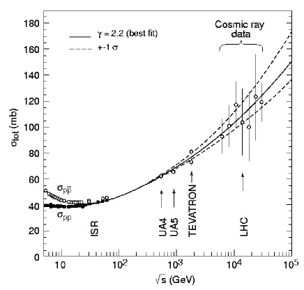
Figure 1: $\sigma_{exp}^{tot}$ from accelerator and from cosmic rays: solid line indicates the best $X^{2}$ fit obtained from a semi-empirical parametrization [6]. The two dashed lines delimitate the region of uncertainty. [ Cosmic ray estimations after [21].

Table 1: $\sigma_{tot}^{\bar{p}p}$ data from high energy accelerators: fits values are from [6].

$\sqrt{s}$ (TeV)		$\sigma_{tot}^{pp}$ (mb)
0.55	Fit	$61.8\pm 0.7$
	UA4	$62.2\pm 1.5$
	CDF	$61.5\pm 1.0$
1.8	Fit	$76.5\pm 2.3$
	E710	$72.8\pm 3.1$
	CDF	$80.3\pm 2.3$
	E811	$71.7\pm 2.0$
16.0	Fit	$111.0\pm 8.0$
40.0	Fit	$130.0\pm 13.0$

Numerical predictions from this analysis are given in Table 1. It should be remarked that at the LHC energies and beyond the predicted $\sigma_{tot}^{pp}$ and $\sigma_{tot}^{\bar{p}p}$ values from the fitting results display relatively high error values ($\Delta\sigma^{tot}_{pred}\geq 8mb$). Also, recent extrapolations for calculations of error bands, based on analysis taking into account cosmic ray and accelerator data, found error values relatively high, as for instance 5 - 7 mb at 14 TeV [24]. We conclude that it is necessary to look for ways to reduce the errors and make the extrapolations more precise.

2 HADRONIC $\sigma_{tot}^{pp}$ FROM COSMIC RAYS

Cosmic ray experiments give us $\sigma_{tot}^{pp}$ in an indirect way: we have to derive it from cosmic ray extensive air shower (EAS) data. But, as summarized in [1] and widely discussed in the literature, the determination of $\sigma_{tot}^{pp}$ is a rather complicated process with at least two well differentiated steps. In the first place, the primary interaction involved in EAS is proton-air; what it is determined through EAS is the $p$-inelastic cross section, $\sigma_{inel}^{p-air}$, through some measure of the attenuation of the rate of showers, $\Lambda_{m}$, deep in the atmosphere:

$$\Lambda_{m}=k\lambda_{p-air}=k\ \frac{14.5m_{p}}{\sigma_{inel}^{p-air}}$$ (4)

The $k$ factor parameterizes the rate at which the energy of the primary proton is dissipated into electromagnetic energy. A simulation with a full representation of the hadronic interactions in the cascade is needed to calculate it. This is done by means of Monte Carlo simulations [25, 26, 27]. Secondly, the connection between $\sigma_{inel}^{p-air}$ and $\sigma_{tot}^{pp}$ is model dependent. A theory for nuclei interactions must be used. Usually is Glauber’s theory [28, 29]. The whole procedure makes hard to get a general agreed value for $\sigma_{tot}^{pp}$. Depending on the particular assumptions made the values may oscillate by large amounts, from as low as $122\pm 11$ at $\sqrt{s}=30$ TeV quoted by the Fly’s Eye group [22, 23] or $133\pm 10$ mb by the Akeno Collaboration [21], both at $\sqrt{s}=30$, to $162\pm 38$ mb nearly $\sqrt{s}=30$ ( around $160-170$ mb $\sqrt{s}=40$ TeV), [30] and even as high as $175_{-27}^{+40}$also at $\sqrt{s}=40$ TeV [31] . In the last cases, and even taking into account the large quoted errors, the values for $\sigma_{tot}^{pp}$ are hardly compatible with the values obtained from the extrapolations of current accelerator data.

From this analysis the conclusion is that cosmic ray estimations of $\sigma_{tot}^{pp}$ are not of much help to constrain extrapolations from accelerator energies. Conversely we could ask if a trustable extrapolation based on accelerator data could not be used to constrain cosmic ray estimations.

3 A MULTIPLE-DIFFRACTION APPROACH FOR EVALUATION OF $\sigma_{tot}^{pp}$

Let us tackle the mismatching between accelerator and cosmic ray estimations using the multiple-diffraction model applied to hadron-hadron scattering [32]. The elastic hadronic scattering amplitude for the collision of two hadrons A and B, neglecting spin, is described as

$$F(q,s)=i\int_{0}^{\infty}b\ db\left[1-e^{i\xi(b,s)}\right]J_{o}(qb)$$ (5)

where $\xi(b,s)$ is the eikonal, $b$ the impact parameter, $J_{o}$ the zero-order Bessel function and $q^{2}=-t$ the four-momentum transfer squared. In the first Multiple Diffraction Theory the eikonal in the transferred momentum space is proportional to the product of the hadronic form factors $G_{A}$ and $G_{B}$ (geometry) and the averaged elementary scattering amplitude among the constituent partons $f$ (dynamics), and can be expressed at first order as $\xi(b,s)=C_{A,B}\left<G_{A}G_{B}f\right>$, where the proportional factor $C_{A,B}$ is the free parameter known as the absorption factor and the brackets denote the symmetrical two-dimensional Fourier transform. A connection between theory and experiment may be obtained by means of hadronic factors and elementary parton-parton amplitudes, which are not physical observable. However with the help of the optical theorem $\sigma_{tot}^{pp}$ may be evaluated in terms of the elastic amplitude $F(q,s)$:

$$\sigma_{tot}^{pp}=4\ \pi\ ImF(q=0,s)$$ (6)

$\sigma_{tot}^{pp}$ is a physical observable, the other two physical observable are the differential cross section and $\rho$ expressed respectively as

$${d\sigma\over{dq^{2}}}={\pi\mid{F(q,s)}\mid^{2}}$$ (7)

and

$${\rho}={\ ReF(q=0,s)\over{\ ImF(q=0,s)}}$$ (8)

Multiple-diffraction models differ one from another by the particular choice of parameterizations made for $G_{A}$ and $G_{B}$ and the elementary amplitude $f$. In the case of identical particles, as is our case, $G_{A}=G_{B}=G$. For our purposes we follow the parametrization developed in a highly outstanding work [7] which has the advantage of using a small set of free parameters, five in total, which are in principle energy dependent: two of them $(\alpha^{2},\beta^{2})$ associated with the form factor

$$G=(1+\frac{q^{2}}{\alpha^{2}})^{-1}(1+\frac{q^{2}}{\beta^{2}})^{-1}$$ (9)

and the other three $(C,a,\lambda)$ associated with the elementary complex amplitude $f$

$$f(q,s)=Ref(q,s)+iImf(q,s)$$ (10)

where

$$Imf(q,s)=C\frac{1-\frac{q^{2}}{a^{2}}}{1-\frac{q^{4}}{a^{4}}}\$$ (11)

and

$$Ref(q,s)=\lambda(s)Imf(q,s)\$$ (12)

so that,

$$ImF(q=0,s)=\ \ \ \ \ \ \ \ \ \ \ \ \ \ \ \ \ \ \ \ \ \ \ \ \ \ \ \ \ \ \ \ \ \ \ \ \ \$$

$$\int_{0}^{\infty}\!\!\left[1-e^{-\Omega(b,s)}\cos\left\{\lambda\Omega(b,s)\right\}\right]b\ db\ J_{o}(q,b)\mid_{q=0}$$ (13)

with the opacity $\Omega(b,s)$ given as:

$$\Omega(b,s)=\int_{o}^{\infty}G^{2}\ Imf(q,s)\ J_{o}(q,b)\ qdq$$ (14)

which explicit expression is:

$$\Omega(b,s)=C\{E_{1}K_{0}(\alpha b)+E_{2}K_{0}(\beta b)+E_{3}K_{ei}(ab)+$$

$$E_{4}K_{er}(ab)+b\left[E_{5}K_{1}(\alpha b)+E_{6}K_{1}(\beta b)\right]\}\$$ (15)

where $k_{0},k_{1},k_{ei},$ and $k_{er}$ are the modified Bessel functions, and $E_{1}$ to $E_{6}$ are functions of the five free parameters. The proton-proton total cross-section is directly determined by the expression

$$\sigma_{tot}^{pp}=4\pi\int_{o}^{\infty}\!\!b\,db\left\{1-e^{-\Omega(b,s)}\cos\left[\lambda\Omega(b,s)\right]\right\}J_{o}(q,b)\mid_{q=0}$$ (16)

expression that was numerically solved in [33], [34]. It should be noted that, according to the principle of Analyticity, the scattering forward amplitude for particle-particle and particle-antiparticle appears from the same analytical function [35]. The behavior of total cross-sections of both reactions is assumed to follow one of the following ways: up to the ISR energies the differences are attributed to Regge contributions, which are expected to disappear at higher energies [5], [36], or on the contrary, differences are interpreted in terms of the Maximal Odderon Hypothesis, which predicts that they increase as the energy overpass the highest energy of the ISR. At this level let us now emphasize an essential point in all which follows. First, we quote the success in the prediction of the value of $\sigma_{tot}^{\bar{p}p}$ at the $S\bar{p}pS$ Collider [10] from the ISR data (mainly pp) using expressions (1) and (2), where $\sigma_{tot}^{pp}$ and $\sigma_{tot}^{\bar{p}p}$ were taken asymptotically equal [20]. Secondly, according to [37] the difference $\Delta\sigma$ between $\sigma_{tot}^{\bar{p}p}$ and $\sigma_{tot}^{pp}$, $\Delta\sigma=\sigma_{tot}^{\bar{p}p}-\sigma_{tot}^{pp}$, up to energies $\leq$ 2000 GeV in the laboratory ($\sim$ 60 GeV in the center of mass) tends toward zero as $s^{-0.56}$, Figure 2. And finally, even if it is argued that $\sigma_{tot}^{pp}$ and $\sigma_{tot}^{\bar{p}p}$ are anyway different for higher energies, we have indicated in Section I that current evidence points the other way round. Taking this triple line of evidence into account, in our multiple-diffraction analysis it is assumed the same behavior for $\sigma_{tot}^{pp}$ and $\sigma_{tot}^{\bar{p}p}$ at high energy. So, here after $\sigma_{tot}^{pp}=\sigma_{tot}^{\bar{p}p}=\sigma_{tot}$. It is noteworthy that some parametrization models, as the RRP [38] predict the same value for both cross sections at $\sqrt{s}>70$ GeV and the same value for the corresponding $\rho$ at $\sqrt{s}>110$ GeV.

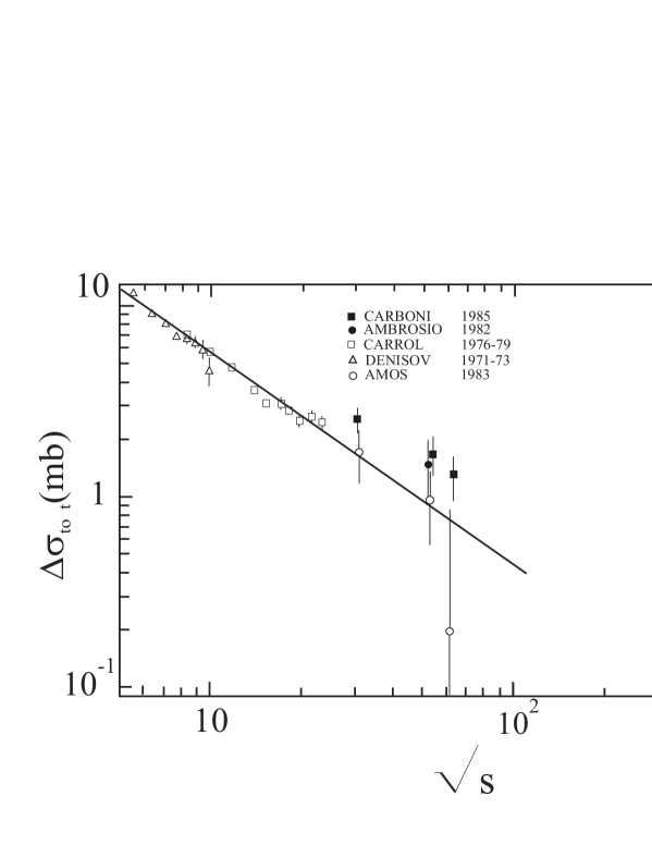
Figure 2: Plot of $\Delta\sigma_{tot}\equiv\sigma^{tot}_{\bar{p}p}-\sigma^{tot}_{pp}\sim s^{-0.56}$ indicating that $\Delta\sigma^{tot}$ tends towards zero up to energies $\sim$ 60 GeV in the center of mass. Data points from [37]

3.1 Evaluation of the Model Parameters

For the evaluation of the free parameters it was assumed, following [7] that two of them are constants: $a^{2}$ = $8.2\ GeV^{2}$ and $\beta^{2}$ = $1.8\ GeV^{2}$. The other three parameters are: $C(s)$ and $\alpha^{-2}(s)$ which determine the imaginary part of the hadronic amplitude [Eq. (11)] and consequently the total cross section [Eq. (6)] , and on the other hand, $\lambda(s)$, which controls the real part of the amplitude [Eq. (12)]. Setting $\lambda(s)$ = $0$ makes the amplitude purely imaginary, so that a zero (a minimum) is produced in the dip region, where only the real part of the amplitude becomes important [39]. We fit experimental data (Fig. 3) of the elastic differential cross section, ${d\sigma\over{dq^{2}}}$, with Eq. (7), choosing the set ($C,\alpha^{-2}$) for which the theoretical and the experimental central values are equated at the precise $-q^{2}$ value where the data show its first minimum (the “dip” position), which coincides with the minimum of the imaginary part of the elastic amplitude. Data of $pp$ differential cross section at $13.8$ and $19.4$ GeV was taken from [40], for $23.5-62.5$ GeV from [41], for $546$ GeV $(\bar{p}p)$ from [42], (for ${\it-t}<0.5$ (GeV/c)²) and [43] (for $0.5\leq{\it-t}\leq 1.55$ (GeVC)²), and for $1800$ GeV from [44](for $0.034\leq{\it-t}\leq 0.65$ (GeVC)²). The procedure is carried out for each one of the energies where there is available accelerator data of ${d\sigma\over{dq^{2}}}$ in the interval $13.8\leq\sqrt{s}\leq 1800$ GeV, as illustrated in Fig 4 and Fig 5. Because error bars of data at the dip position are small the fitting procedure is based on the central values. It must be emphasized that, it is precisely because the minimum of the imaginary amplitude is produced in the dip region, that data at $1800$ GeV is quite suitable to our procedure, since the predicted minimum falls at $t=0.585$ $GeV^{2}$ where there is available data (${d\sigma\over{dt}}=0.0101$). The next data value at $t=0.627$ $GeV^{2}$ shows an slight increase. Furthermore, the shift of the dip region toward lower values of $t$ as the considered energy increases is qualitatively consistent with the expectation relative to the shoulder at $546$ GeV ($t=0.9$ $GeV^{2}$). Once the values of $C(s)$ and $\alpha^{-2}(s)$ are determined for each energy they are introduced, together with the constant parameters $a^{2}$ and $\beta^{2}$ into Eq. (8). Giving values to the parameter $\lambda(s)$ up to obtain the experimental value of $\rho(s)$, we determine the $\lambda$ value for each energy where there is available accelerator data in the same interval $13.8\leq\sqrt{s}\leq 1800$ GeV. The obtained central values of the three energy-dependent free parameters, $C(s)$, $\alpha^{-2}(s)$and $\lambda(s)$ are listed in Table 2. Therefore, the employed method to evaluate the model parameters only requires data of $(d\sigma\over{dt})$ and $\rho(s)$.

Table 2: Values of the parameters $C$, $\alpha^{-2}$, $\lambda$ at each energy. They are obtained by equating the accelerator data and the model prediction for the elastic differential cross-sections and for the parameter $\rho$ in the interval $13\leq\sqrt{s}\leq 62.5$ and $546\leq\sqrt{s}\leq 1800$ GeV.

$\sqrt{s}$	$C(s)$	$\alpha^{-2}(s)$	$\lambda(s)$
(GeV)	(GeV-2)	(GeV-2)
13.8	9.97	2.092	-0.126
19.4	10.05	2.128	-0.043
23.5	10.25	2.174	0.025
30.7	10.37	2.222	0.053
44.7	10.89	2.299	0.079
52.8	11.15	2.350	0.099
62.5	11.42	2.380	0.115
546	16.90	3.060	0.182
1800	21.52	3.570	0.194

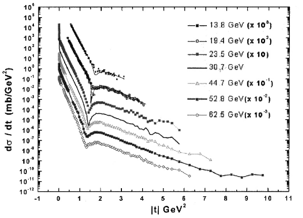
Figure 3: Data of $pp$ differential cross section at $\sqrt{s}\leq 62.5$ according to [40],[41], [42], [43] and [44].

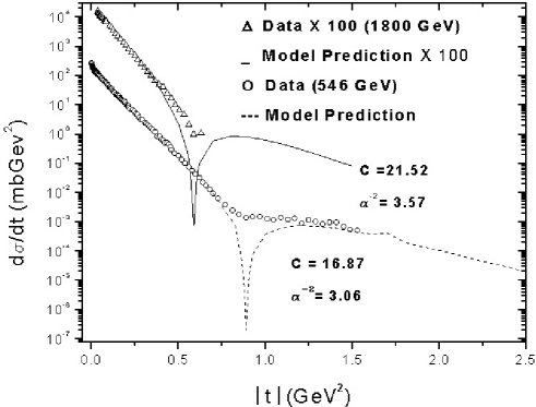
Figure 4: Fits of the predicted imaginary amplitude to data of the $\bar{p}p$ differential cross sections to determine $C(s)$ and $\alpha^{-2}(s)$ by equating experimental and theoretical values at the specific $\mid t\mid$ of the “dip” position for $\sqrt{s}=546GeV$ and $\sqrt{s}=1800GeV$.

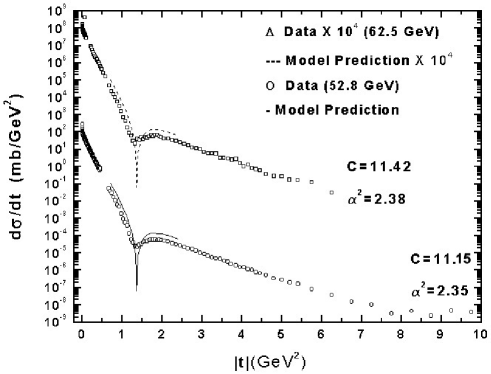
Figure 5: Idem that Fig. 4, for $\sqrt{s}=52.8$ and $\sqrt{s}=62.5GeV$.

4 PARAMETRIZATION FOR EXTRAPOLATION TO HIGH ENERGIES

Concerning the physics behind a parametrization and fitting procedures, it should be emphasized that there is not yet an answer on microscopic basis, i.e., on terms of the QCD theory, because diffractive physics is essentially a non-perturvative phenomenon and confinement is the unsolved problem of QCD. However, on basis to the present model it can be said that the closeness of our fits to the colliders data (ISR, $S\bar{p}pS$ and Tevatron) gives us an indication that the basic tenets of the model are right, as was described for instance in reference [32]. In spite of the approximation made in ignoring crossing symmetry, the parametrization carried out here is not an arbitrary one as will be described below.

On this basis, with the aim of interpolating values at energies where there is no available accelerator data and for extrapolation to higher energies, we proceeded to perform a parametrization of the three energy-dependent free parameters. According to the obtained values of those parameters, as described in Section III-A (Table 2) and following the procedure to be described in Section V, a second-order fitting of the values of $C(s)$ and $\alpha^{-2}(s)$ and a exponential fitting of $\lambda(s)$ has been obtained from the following analytical expressions:

$$C(s)=19.24521-2.86114\ ln(s)+0.22616\ ln(s)^{2}$$ (17)

$$\alpha^{-2}(s)=1.8956-0.03937\ ln(s)+0.01301\ ln(s)^{2}$$ (18)

$$\lambda(s)=0.01686+0.00125\left(1-\ e^{-ln(s/400)/0.18549}\right)+$$

$$0.19775\left(1-\ e^{-ln(s/400)/3.74642}\right)\$$ (19)

Results are displayed in Table 2 and illustrated in Figures (6) -(8) as the central solid lines.
However, it must be taken into account that the reliability of the functional parameterizations for extrapolations must have a physical support, since it is clear that several parameterizations that may describe correctly the set of data in the experimental range $13.8\leq\sqrt{s}\leq 1800$ GeV, may not be consistent any more, but differ substantially when extrapolated to high energies. Therefore, some restrictions must be imposed in the selection of parameterizations according to the physical information available. As we mentioned before, our fittings of $C(s)$ and $\alpha^{-2}(s)$ in the limited experimental range were based on experimental data of the differential cross-section and the $\rho(s)$ parameter, obtaining values that increase with energy (Table 2) with positive concavity (Figs. 6-7). Experimentally, total cross-sections increase with energy like $\ln(s)$ or $\ ln^{2}(s)$ in the concerned energy range, and on the other hand, soft processes are expected to have a $\ln(s)$ behavior: from the optical theorem, the interdependence between the free parameters and the physical observable (Eq. 6) may be connected with the unitary condition, for which lowest order cross-sections within the frame of gauge field theories present $\ln(s)$ terms [45]. Based on our fittings and extrapolation results and on the previously mentioned constraints, the presence of $\ln(s)$ terms in the two-energy dependent parameters $C(s)$ and $\alpha^{-2}(s)$ is a natural consequence, and therefore the hypothesis of polynomial functions of $\ln(s)$ seems a reasonable one.

Concerning the parameter $\lambda(s)$ let us pointed out that a basic property of the Glauber Multiple Diffraction Model is to associate elastic scattering cross-sections of nucleons with the scattering amplitude of their composite partons [32]: within this framework, the proportionality between real and imaginary parts of the parton-parton amplitudes (Eq. 12), $\lambda(s)=Ref(q,s)/Imf(q,s)$ implies that $\lambda(s)$ at the partonic scale behaves similarly as $\rho(s)$ does at the hadronic scale. The influence of $\lambda(s)$ on the hadronic amplitude has been empirically analyzed in [7], showing that if $\lambda(s)$ increases (or decreases) also $\rho(s)$ increases (or decreases) (Fig. 9), and $\lambda(s)=0$ at the same energy value where $\rho(s)=0$. However, due to the lack of $\rho(s)$ data above the experimental energy range used in this work, the parametrization of $\lambda(s)$ at high energies is based on the conventional assumption that beyond $\sqrt{s}\sim 100$ GeV, $\rho(s)$ presents a maximum and then goes asymptotically to zero [14], the rate of convergence depending on model particularities. Based on this consideration and on the empirical behavior of $\lambda(s)$, shown in Table 2, we propose the parametrization given in Eq. (19), where $S_{o}=400$ GeV² is the value at which $\lambda(s)$ converges to zero, and the numerical coefficients control the maximum and asymptotic behavior.

Let us now remind that blackening and expansion are very well known properties of elastic scattering. Within the context of the present empirical analysis, blackening and expansion are related to the elementary parton-parton amplitude and the hadronic form factors through the energy-dependent parameters $C(s)$ and $\alpha(s)$ respectively. Since in the very forward direction the scattering amplitude is basically of diffractive nature, the eikonal becomes a purely imaginary one, then for hadron-hadron $\xi(b,s)=C(s)\left<G^{2}Imf(q,s)\right>=Im\Omega(b,s)$, so that in terms of Eqs. (9) and (11) the opacity satisfies $\Omega(b,s)\geq 1$, and the free parameter $C(s)$ behaves as an absorption factor (optical theorem). On the other hand, the free parameter $\alpha(s)^{2}$ may be connected to the hadronic radius [7] as $R^{2}(s)=-6[dG(q,s)/dt]_{t=0}$. Then, from Eq. (9)

$$R^{2}(s)=0.2332\left[\frac{1}{\alpha^{2}(s)}+\frac{1}{\beta^{2}(s)}\right](fm)^{2}.$$

Therefore, from Eq. (18) and the adopted value $\beta^{2}=1.8$ GeV² the radius is an increasing function of energy and such a behavior is connected to the expansion effect. The result is that hadrons become blacker and larger with energy increase, consistently with the so called “Bell Effect” [46]. Since the hadronic scattering amplitude is purely imaginary the free parameters may be associated with the physical observable by means of Eq. (6) - (7).

5 THE EXTRAPOLATION PROCEDURE

The procedure followed to arrive to the predictions of $\sigma_{tot}^{pp}$ at high energies with statistic confidence intervals based on the forecasting method described in Appendix A is the next: -(i) using the values displayed in Table 2, we established prediction equations of the type of eq. (A4) within the data range and eq. (A6) ) out of the range, for each of the energy-dependent parameters: (ii) using the least squares method in matrix formalism, as described in the Appendix (eqs. A10-A12) we obtained the constants $\hat{\beta}_{0},\hat{\beta}_{1},\hat{\beta}_{2}$ for each one of the parameters. The autocorrelation constant was determined as described in [47, 48], (iii) with the obtained values the central values of the three parameters were derived (eqs. 17-19), leading to a second-order fitting of the values of $C(s)$ and $\alpha^{-2}(s)$ and a exponential fitting of $\lambda(s)$; results are shown in Table 2, (iv) we evaluated the variance for each one of the new forecasted value (eq. A14) , (v) by means of eqs. (A15)-(A16) we estimated the confidence intervals for each one of the interpolated-extrapolated values, such that by a fitting of the extreme values of these confidence intervals we have built the error bands of each one of the parameters, what is shown in Figs. (6)-(8), (vi) the Central values of $\sigma_{tot}^{pp}$ for each point are obtained by means of the introduction in eqs. (15)-(16) of the values of $C(s)$, $\alpha^{-2}(s)$ and $\lambda(s)$ (displayed in Table 2), (vii) finally, the overall confidence band for the predicted $\sigma_{tot}^{pp}$ is obtained, not from eqs. (A15)-(A16), but from the substitution of the extreme values of the error bands of the three energy-dependent parameters into eqs. (15)-(16), followed by the corresponding fittings (Figs. 10-11).

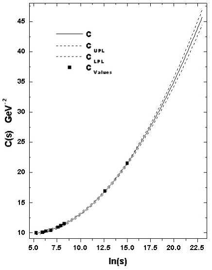
Figure 6: The parameter $C(s)$ from Table 2 with its confidence interval.

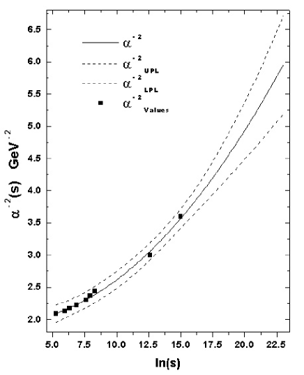
Figure 7: The parameter $\alpha^{-2}(s)$ from Table 2 with its confidence interval.

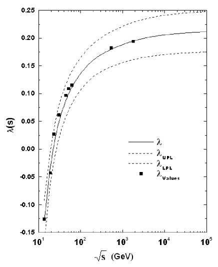
Figure 8: The parameter $\lambda(s)$ from Table 2 with its confidence interval.

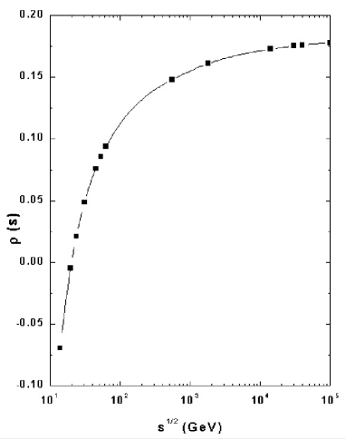
Figure 9: Data behavior of the parameter $\rho(s)$ at $\sqrt{s}\leq 62.5$

Table 3: Fitted values (interpolation and extrapolation) of $C(s)$, $\alpha^{-2}(s)$ and $\lambda(s)$ .

$\sqrt{s}$	$C(s)$	$\alpha^{-2}(s)$	$\lambda(s)$
(GeV)	(GeV-2)	(GeV-2)
13.8	9.9039	2.0945	-0.12816
19.4	10.082	2.1469	-0.02848
23.5	10.225	2.1798	0.00975
30.7	10.474	2.2296	0.04942
44.7	10.923	2.3075	0.08786
52.8	11.159	2.3451	0.10064
62.5	11.421	2.3849	0.11172
546	16.872	3.0634	0.18035
1800	21.518	3.5685	0.19501
14000	32.239	4.6555	0.20703
16000	33.056	4.7359	0.20749
30000	37.102	5.1298	0.20927
40000	39.062	5.3188	0.20993
100000	45.757	5.9568	0.21153

6 RESULTS

Data of the total cross sections with their respective errors are summarized in Table IV. At $\sqrt{s}\leq 62.5$ GeV data was taken from [41], for $546$ GeV from [10]. For the value at $1800$ GeV there exist three different measurements: the value of the CDF collaboration $(80.3\pm 2.24mb)$ [12], the value of the E710 collaboration $(72.8\pm 3.1mb)$ [11] and the value of the E811 collaboration $(71.7\pm 2.02mb)$ [13]. There is a high controversy on whether the correct value is that of the CDF collaboration or those lower values of the E710 collaboration and the E811 collaboration, mainly related to the estimation of the different backgrounds. For instance the CDF Collaboration has decided to use only their $\sigma_{tot}^{pp}$ value to quote luminosity values for all of their physics program [50] whereas the other Tevatron Collaboration, D0, has adopted the average of the three measurements [50]. For the goal of this work, one of us (J.V.) suggested to follow this second option and use the arithmetic weighted mean of the three values, ($74.91\pm 1.35$ mb). The consequence in our results of the employment of the values of those three collaborations is mentioned in the next section.

We quote in Table IV the values of the predicted $\sigma_{tot}^{pp}$ for two different energy intervals: $\sigma_{tot}^{1800}$, ($13.8\leq\sqrt{s}\leq 1800$ GeV), and $\sigma_{tot}^{546}$, ($13.8\leq\sqrt{s}\leq 546$ GeV). Figure 10 represents graphically the first case together with cosmic ray data. For further discussion, we include in Table IV predicted values from two standard accelerator-based data extrapolations: the first one, $\sigma^{[54]}_{546}$ makes a fit to all $\sigma_{tot}^{pp}$ and $\sigma_{tot}^{\bar{p}p}$ data in the interval $10\leq\sqrt{s}\leq 546$ GeV using expression (2) [51], and the second one, $\sigma^{[5]}_{\rho}$ (Fig. 1), in the same energy range, makes the simultaneous fit to all $\sigma_{tot}^{pp}$, $\sigma_{tot}^{\bar{p}p}$, $\rho_{tot}^{pp}$ and $\rho_{tot}^{\bar{p}p}$ data through the method described in Section I, [6] .

Table 4: Central, upper and lower values for $\sigma_{tot}$ obtained with the forecasting method. The $\sigma^{1800}_{tot}$, $\sigma^{546}_{tot}$, $\sigma^{62.5}_{tot}$ columns includes data up to 1800, 546, 62.5 GeV respectively. The quoted $\sigma_{546}^{[54]}$ and $\sigma_{\rho}^{[5]}$ values are from [51], and[6] respectively.

$\sqrt{s}$ (GeV)	$\sigma^{exp}_{tot}$ (mb)	$\sigma^{1800}_{tot}$ (mb)	$\sigma_{546}^{[54]}$ (mb)	$\sigma^{546}_{tot}$ (mb)	$\sigma_{\rho}^{[5]}$ (mb)	$\sigma^{62.5}_{tot}$ (mb)
13.8	38.36 $\pm$ 0.04	$38.29_{-0.98}^{+1.06}$	- - -	$38.30_{-0.92}^{+0.94}$	- - -	$38.51_{-0.56}^{+0.62}$
19.4	38.97 $\pm$ 0.04	$38.92_{-0.97}^{+0.98}$	- - -	$38.82_{-0.87}^{+0.88}$	- - -	$38.82_{-0.54}^{+0.59}$
23.5	38.94 $\pm$ 0.17	$39.44_{-0.96}^{+0.97}$	- - -	$39.44_{-0.86}^{+0.88}$	- - -	$39.26_{-0.58}^{+0.62}$
30.7	40.14 $\pm$ 0.17	$40.34_{-0.95}^{+0.99}$	- - -	$40.37_{-0.88}^{+0.88}$	- - -	$40.15_{-0.61}^{+0.66}$
44.7	41.79 $\pm$ 0.16	$41.93_{-0.96}^{+1.06}$	- - -	$42.00_{-0.92}^{+0.93}$	- - -	$41.93_{-0.62}^{+0.66}$
52.8	42.67 $\pm$ 0.19	$42.76_{-0.98}^{+1.09}$	- - -	$42.84_{-0.94}^{+0.95}$	- - -	$42.93_{-0.64}^{+0.69}$
62.5	43.32 $\pm$ 0.23	$43.67_{-0.99}^{+1.13}$	- - -	$43.77_{-0.97}^{+0.98}$	- - -	$44.05_{-0.72}^{+0.78}$
546	61.5 $\pm$ 1.5	$61.62_{-0.94}^{+1.58}$	- - -	$61.78_{-1.29}^{+1.33}$	- - -	$69.39_{-7.4}^{+8.4}$
1800	74.91 $\pm$1.35(∗)	$76.17_{-1.07}^{+2.02}$	76.7 $\pm$ 4.0	$76.00_{-2.34}^{+2.41}$	76.5 $\pm$ 2.3	$91.74_{-14.7}^{+16.9}$
14000	- - -	$108.27_{-3.17}^{+4.72}$	112 $\pm$ 13.0	$106.5_{-6.55}^{+6.56}$	- - -	$143.86_{-33.5}^{+38.6}$
16000	- - -	$110.67_{-3.40}^{+5.00}$	- - -	$108.7_{-6.94}^{+6.94}$	111.0 $\pm$ 8.0	$147.85_{-35.1}^{+40.3}$
30000	- - -	$122.41_{-4.62}^{+6.40}$	- - -	$119.6_{-8.96}^{+8.83}$	- - -	$167.64_{-42.6}^{+48.9}$
40000	- - -	$128.05_{-5.27}^{+7.08}$	- - -	$124.7_{-9.97}^{+9.83}$	130.0 $\pm$ 13.0	$177.23_{-46.3}^{+53.1}$
100000	- - -	$147.14_{-7.68}^{+9.63}$	- - -	$142.0_{-13.7}^{+13.33}$	- - -	$210.06_{-59.1}^{+67.6}$

(*) This value is the weighted arithmetic mean of the E710 ($72.8\pm 3.1$ mb), CDF ($80.3\pm 2.3$ mb) and E811 ($71.7\pm 2.0$) values.

7 DISCUSSION

To start with, let first examine what happens when our main assumption, the asymptotic equality of $\sigma_{tot}^{pp}$ and $\sigma_{tot}^{\bar{p}p}$, is not used. Analysis of Figure 11 shows that if we limit our fitting calculations to the accelerator domain $\sqrt{s}\leq 62.5$ GeV, where $\sigma_{tot}^{pp}$ data exist, the extrapolation at cosmic ray energies produces an error band so large that practically any cosmic ray result become compatible with results at accelerator energies. It can be seen that in this case the $\sigma_{tot}^{pp}$ values obtained when extrapolated to ultra high energies seem to confirm the highest quoted values of the cosmic ray experiments [30, 31]. Also it can be noted that such extrapolation to ultra high energies may claim not only agreement with the analysis carried out in [30] and the experimental data of the Fly’s Eye [31], but even with the Akeno collaboration [21], because their experimental errors are so big that they overlap with the errors reported in [31], and of course falling within the predicted error band for that case $\sqrt{s}\leq 62.5$ GeV (Fig. 11). If that were true, it would imply the extrapolations cherished by experimentalists are wrong. But the prediction shown in Fig. 11 gives $\sigma_{tot}^{pp}=$ 69 mb at the CERN $S\bar{p}pS$ Collider ($546$ GeV), and $91.6mb$ at the Fermilab Tevatron ($1.8$ TeV). Comparing with Table I we see that the measured $\sigma_{tot}^{\bar{p}p}$ at $546$ GeV is smaller than the predicted $\sigma_{tot}^{pp}$ by near $8$ mb, and in the case of $1.8$ TeV by more than $15$ mb, which no available model is able to explain [15]. However when our main hypothesis, $\sigma_{tot}^{\bar{p}p}=\sigma_{tot}^{pp}$ asymptotically is used, then the existing $\sigma_{tot}^{\bar{p}p}$ data at higher accelerator energies may safely be included. This allows to enlarge by a great amount the lever arm for the extrapolation and both the predicted values and the error band change considerably. This can be clearly seen in Fig. 10, as well as in Table IV, where we have added the available $\sigma_{tot}^{\bar{p}p}$ up to 0.546 TeV (the $\sigma^{546}_{tot}$ column) and up to 1.8 TeV (the $\sigma^{1800}_{tot}$ column). Now the predicted value of $\sigma_{tot}^{pp}$ from our extrapolation $\sigma^{1800}_{tot}$, for instance at $\sqrt{s}=40$ TeV, $\sigma_{tot}^{pp}=128.0_{-5.27}^{+7.08}$ mb, is seen incompatible with those in [30, 31] by several standard deviations, though no so different to the Fly’s Eye or Akeno results and the predicted value in [6].

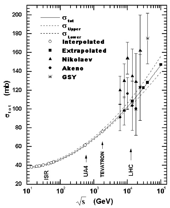
Figure 10: Prediction of the total cross-section using data up to 1800 GeV (solid line), $\sigma^{1800}_{tot}$. The error band (dashed lines) is obtained by the forecasting method.

Concerning the quoted error bands, in sections V, it has been shown in the Appendix that due to the inclusion of Residual Correlations in the Forecasting method, this is always a high precise technique whatever the employed parametrization model, but this systematic advantage occurs, provided we are dealing with the same parametrization model under the same input conditions. Therefore, it must be emphasized that it is not valid a comparison between different statistical techniques on basis to different parametrization models, or running of the same parametrization with different input values. However, in spite of this, we would like to make a consideration of strictly qualitative nature, in the sense that other parameterizations [6], [51] with similar input quantities (for instance $\rho$ and ${d\sigma\over{dt}}$) lead to central values that are only slightly higher than ours, whereas the quoted errors are larger than ours by nearly a factor of 3, as can be seen in Table 4, or in Fig. 4 and Fig.10. For instance, the quoted error in the fit $\sigma_{tot}^{1800}$ at 100 TeV in the center of mass (which corresponds to $\simeq 10^{19}$ eV in the lab), $147_{-7.68}^{+9.63}$, is comparable (or even better) to the error obtained at much more lower energies in other works as can be seen in Table IV, at $16$ TeV and $14$ TeV ($\simeq 10^{17}$ eV in the lab), corresponding to the energy range of future LHC CERN Collider. Another parametrization which predictions of the cental values are not so different of ours, is that of the Ensemble A, of the work [52, 53]. Obviously, the previous analysis is only of qualitative nature, but it is however quite important because such a discussion opens new interrogatives: - though, it is clear that from statistic theory the forecasting technique is a highly precise method (section V, Appendix and references therein) , its advantage is, however, only a second order effect when applied to the same conditions (as shown in Eqs. 20 and 27), why this higher preciseness seems to be amplified when qualitative comparisons are made with a different parametrization model the same different inputs?, is it because the employed parametrization model is better?. It is clear that the answer must be based on a deep quantitative analysis, by applying the forecasting method to different parametrization models of total cross-section, in order to discern which model is more confident, and from there to draw more reliable physical inferences. Such an analysis is out of the scope of the present paper, and will be the subject of a forthcoming work.

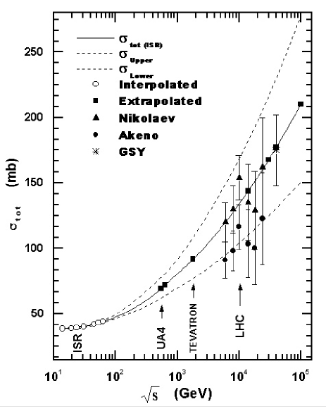
Figure 11: Prediction of the total cross-section using $pp$ data up to 62.5 GeV (solid line). The error band (dashed lines) is obtained by the forecasting method.

8 CONCLUSIONS

It has been shown in this work that highly confident predictions of high energy $\sigma_{tot}^{pp}$ values are strongly dependent on the energy range covered by experimental data and the available number of those data values. In particular, if we limit our study of determining $\sigma_{tot}^{pp}$ at cosmic ray energies from extrapolation of $\sigma_{tot}^{pp}$ accelerator data in the range $\sqrt{s}\leq 62.5$ GeV, then the obtained results are compatible with most of cosmic ray experiments and other prediction models, because the predicted error band is so wide that covers their corresponding quoted errors (Fig. 11). However, as the included data in our calculations extends to higher energies, including $\sigma_{tot}^{\bar{p}p}$ data up to 1.8 TeV, that is, when all experimental available data is taken into account, the range of possibilities is much reduced. It should be noted that our predictions are compatibles with other prediction studies [6]. Taken all this results at face value, i.e. as indicating the most probable $\sigma_{tot}^{pp}$ value, we conclude that if predictions from accelerator data are correct, hence it should be of great help to normalize the corresponding values from cosmic ray experiments, as for instance by keeping the ($k$) parameter as a free one. The $k$ value found will greatly help the tuning of the complicated Monte Carlo calculations used to evaluate the development of the showers induced by cosmic rays in the upper atmosphere. If extrapolations from our parametrization model are correct this would imply that $\sigma_{p-air}^{inel}$ should be smaller than usually considered, which would have important consequences for development of high energy cascades. Though it is quite clear that the statements of this work are based on the assumption $\sigma_{tot}^{pp}$ = $\sigma_{tot}^{\bar{p}p}$ at energies in the range 546 $\leq\sqrt{s}\leq$ 1800 GeV, we claim that this “enigma” will be solved by the forthcoming new very high energy colliders. The new Relativistic Heavy Ion Collider (RHIC) which has become operational at Brookhaven, should produce a value of $\sigma_{tot}^{pp}$ at $\sqrt{s}=500$ GeV very soon, allowing a comparison with the $\sigma_{tot}^{\bar{p}p}$ measured value at $\sqrt{s}=546$ GeV. Later on, the LHC should give us a $\sigma_{tot}^{pp}$ value at $\sqrt{s}=14$ TeV. If it could be run at 2 TeV, a direct comparison between its $\sigma_{tot}^{pp}$ value and the $\sigma_{tot}^{\bar{p}p}$ found at the Tevatron could be done. Additionally, experiments such as the HiRes [2] and the Auger Observatory [3] will bring new highlights to solve the puzzle about extrapolations to cosmic ray energies, i.e. whether the real values of $\sigma_{tot}$ are described by parameterizations consistent with a fast energy rise at high energies, which we may called “cosmic result” or by a slower rise in energy, the “accelerators result” as is the case presented in this paper. We argue that instead of looking for a new physics based on “exotic” events to explain very fast rise in energy of $\sigma_{tot}$, what we need is highly trustable data at intermediate energies ($2\leq\sqrt{s}\leq 15$ TeV) to use them as confident lever arms for extrapolations, to approach in this way to a more accurate description of $\sigma_{tot}$ at cosmic ray energies. In summary, extrapolations from accelerator data cannot be disregarded to constraint cosmic ray estimations.

Appendix A CONFIDENCE INTERVALS OF THE MODEL PREDICTION

The ability of a statistical method to reproduce data of any physical quantity with high precision gives the pattern for the prediction of out of the range data. In the context of $pp$ and $\bar{p}p$ hadronic total cross sections at very high energies a great deal of work has been done out of the energy range of accelerators: predictions are usually compared to cosmic ray data producing a disagreement which explanation has also been widely discussed in the literature. Such comparison depends critically of a highly confident band of uncertainty for any parametrization model. The validity of any statistical method to predict a given physical quantity out of the range values, “prognosis” (extrapolation) depends on its precision to reproduce the employed data (interpolation). A fundamental task of any prediction method is to minimize the error band of the predicted set of values. In the specific case of $\sigma_{tot}$ what is searched is to obtain a prediction beyond the energy range of the employed data with the minimum of dispersion. In this context, popular techniques are derived from the statistical theory known as Regression Analysis either on the multiple regression approach or on the simplest version, a simple regression analysis, both based on the method of Least Squares. Among the important indicators of any statistical method within the frame of the present work there is the confidence level (C.L.) and the confidence intervals (e.g., [49]).

For a given phenomenon characterized by an independent variable ( x ) that generates a response variable ( y) regression analysis supplies a procedure to estimate the corresponding statistics: to fit a set of data of the phenomenon in between the known points (interpolation), to estimate $(\bar{y})$ the mean value of (y), to predict a future value of (y) beyond the known points (prognosis out of the data range) for a given value of (x) ), and to build a confidence interval around each of the estimated or prognosticated values (for instance [54, 55]). In its general form the dependent variable (y) can be written as a function of ${\it k}$ independent variables $x_{1},x_{2},....x_{\it k}$, where the variables $x_{j}$ may represent powers of these variables, cross products of the variables, or even to present a parametric dependence of other variable (see for instance [56]). Statistic techniques of regression analysis are based on the minimization of the quadratic sum of data deviations with respect to the employed mathematical model of prediction: for a given distribution of residuals $R_{i}=y_{i}-\bar{y}_{i}$ a full set of confidence indicators are generated, where typical error bands (belts) for extrapolations up to ${\it m}$ steps beyond the last $n-esim$ experimental point is given as

$$ErrorB=\bar{y}_{n+m}\pm t_{\delta/2}^{k-p}S_{d}$$ (20)

where $S_{d}^{2}$ is the variance, defined as the square of the standard deviation (usually called the standard error of estimate), $\bar{y}_{n+m}$ is the corresponding Central prediction and $t^{\{k-p\}}_{\{\delta/2\}}$ denotes the Probability Density Function (p.d.f.) known as the Student’s $\{\bf{t}\}$ -distribution for the $k$ values of the independent variables with $p$ degrees of freedom, and a confidence coefficient $\delta/2$. However, the previous generalization does not incorporates effects related to the position of the experimental values of (y) around the employed Central Value, that is the correlation among residuals that generates the regression model [56]. In other words, it is assumed no interaction terms, implying that each of the independent variables affects the response $(y)$ independently of the other independent variables and the error $\epsilon$ associated with any one $(y)$ value is independent of the error associated with any other $(y)$ value. Such an omission of the residuals correlation leads to a notorious modification of the statistic estimators [38].

A.1 The Forecasting Method

The previous limitation, mentioned above, can be surmounted by identifying the obtained data set $(x_{1i},x_{2i},x_{3i}......x_{ki};y_{i})$ with a time series, and then to proceed an evaluation of the correlation among consecutive residuals (the so called autocorrelation procedure, from which the simplest one is the autoregressive 1st-order model). The forecasting statistic method is based on autocorrelation models which allows for the evaluation of the correlation among consecutive residuals, out and in the set of data by means of an iterative process [56]. In general, this procedure modifies the fitting constants of the model, the estimated variance of residuals and minimizes the width of the error intervals for interpolation or prognosis (extrapolation), increasing in this way the confidence level $(CL)$ of predictions [56]. To quantify the effect that has the autocorrelation of residuals on the regression model and associated estimators, let us represent such a model by a response variable $y=E(y)+\epsilon$ where

$$E(y)=\beta_{0}+\beta_{1}x_{1}+\beta_{2}x_{2}+........+\beta_{k}x_{k}$$ (21)

represents the deterministic component of the proposed regression model, $x_{1},x_{2},...,x_{k}$ are the independent variables, that are known without error, and may represent higher order terms and even functions of variables as long as the function do not contain unknown parameters, $\beta_{1},\beta_{2},....,\beta_{k}$ are the unknown coefficients to be determined by the least squares method, representing the contribution of the independent variables $x_{i}$ and $\epsilon$ represents the random error component. For the evaluation of residuals $R_{i}=y_{i}-E(y_{i})$ it is assumed they have a normal distribution which mean is zero and the variance is constant. In the autoregressive model of 1st-order each residual $R_{i}$ is related with the previous one as

$$R_{i}=\phi R_{i-1}+{\it r_{i}}$$ (22)

where $\phi$ is the autocorrelation constant among the residuals $(\mid\phi\mid<1)$, [47, 48], and ${\it r_{i}}$ in this case is a Residual called white noise, uncorrelated of any other Residual component. The incorporation of the effect of autocorrelation of residuals to the solution of the regression problem through equation (A2) leads to a modification of the regression constants and the corresponding variance: using the set of data, the estimation of the $k+1$ regression constants of eq. (A2) and the constant $\phi$ are obtained from the autocorrelation model according to the following interpolation equation for the response variable $\hat{y}_{i}$:

$$\hat{y}_{i}=\hat{\beta}_{0}+\hat{\beta}_{1}x_{1,i}+\hat{\beta}_{2}x_{2,i}+........\hat{\beta}_{k}x_{k,i}+\hat{\phi}\hat{R}_{i-1}$$ (23)

where $i=1...n$, $x_{k,i}$ represents the independent variable $x_{k}$ corresponding to the point $(i)$, the small hat indicates the estimated values, that is they have been evaluated, and the mean of the residual white noise has been taken as $\bar{\it r}_{n+1}=0$. The prediction of values beyond the n-esim data value, beginning for instance with $y_{n+1}$, is then given as

$$y_{n+1}=\hat{\beta}_{0}+\hat{\beta}_{1}x_{1,n+1}+\hat{\beta}_{2}x_{2,n+1}+........+\hat{\beta}_{k}x_{k,n+1}+R_{n+1}$$ (24)

where $x_{k,n+1}$ represents the independent variable $x_{k}$ corresponding to the point $(n+1)$. The forecast (prognostic) for the response variable $\hat{y}_{n+1}$ is :

$$\hat{y}_{n+1}=\hat{\beta}_{0}+\hat{\beta}_{1}x_{1,n+1}+\hat{\beta}_{2}x_{2,n+1}+........+\hat{\beta}_{k}x_{k,n+1}+\hat{\phi}\hat{R}_{n}$$ (25)

Similarly, for a posterior value $\hat{y}_{n+2}$,

$$\hat{y}_{n+2}=\hat{\beta}_{0}+\hat{\beta}_{1}x_{1,n+2}+\hat{\beta}_{2}x_{2,n+2}+........+\hat{\beta}_{k}x_{k,n+2}+{(\hat{\phi})}^{2}\hat{R}_{n}$$ (26)

and so on successively, that is the forecasting of values out of the range of data is an iterative process where every new prognostic make use of the previous Residual. Unfortunately, as we move more and more far from the last data value, the potential error increases due to possible changes in the structure of the regression model, or changes in the variance value as the prognostic are taking place. The later can be surmounted by estimating the variance associated with each prognostic (forecasting variance) through the correlation constant $\phi$; therefore, according to the autoregressive model of 1st-order within the data range up to the data $n$ we have a constant variance $S_{f}^{2}$, and for one step out of the data range (i.e., $n+1$) the corresponding variance is $S_{f,n+1}^{2}=S_{f}^{2}[1+\phi^{2}]$, whereas for two steps beyond $(n+2)$ the forecasting variance is $S_{f,n+2}^{2}=S_{f}^{2}[1+\phi^{2}+\phi^{4}]$ and for $m$ steps beyond the range $(n+m)$ the forecasting variance is $S_{f,n+m}^{2}=S_{f}^{2}[1+\phi^{2}+\phi^{4}+....+\phi^{2(m-1)}]$. On this basis, for a prediction interval with a confidence of $100(1-\delta)\%$ and a type $t-student$ distribution, the amplitude of the prognostic intervals for $(n+m)$ steps beyond the $n-esim$ data value is given in [56], as:

$$ErrorB=\hat{y}_{n+m}\pm t_{\delta/2}^{k-p}\sqrt{S_{f}^{2}[1+\phi^{2}+\phi^{4}+....+\phi^{2(m-1)}]}$$ (27)

Due to the incorporation of the autocorrelation of residuals, the error bands evaluated in this way gives a higher Confidence Level than other methods of Regressive Analysis which ignore this effect [56], what is translated in a width decrease of the prediction intervals as a consequence of the decrease of the estimated variance(e.g., Table 9.7 in [56]). It must be emphasized that technically the meaning of the error bars in different methods derived from regression analysis is exactly the same , since they quantify the level of confidence (C.L.), that is, they express the probability that the “true answer” can be placed with $100(1-\delta)\%$ of probability within the interval of aleatory measurements, or predictions, when other measurement is done under the same conditions. However, even if the concept is the same , every method predicts a different value of (C.L.): in the particular case of the forecasting, the essential point is that it uses the additional factor of the autocorrelation among residuals, what improves (1) the Central prognostic value and (2) the amplitude of the confidence intervals (error bars), whose narrowing is translated precisely in a high level of confidence [56].

A.2 Matrix Approach in Regression Analysis

This forecasting method is based on the multiple regression theory and consists in determining a prediction equation for a quantity $y$ (dependent variable), that in turns depends on $k$ independent variables ($x_{i}$), that is

$$E(y)=\sum_{i=0}^{k}\beta_{i}f_{i}(x_{i})$$ (28)

(with $f_{o}(x_{o})=1$) , where $f_{i}$ are arbitrary functions of $x_{i}$, and $\beta_{i}$ are the fitting constants. In the generalized version the variable $x_{i}$ may depend on other parameters, i.e., $x_{i}=x_{i}(s,t,..)$. Therefore, the application of a multiple regression model to a given problem leads to trace a system of $n$ equations with $n$ incognitos, so that its solution is better obtained through a matrix formalism. Denoting with $Y$ the matrix of $(n\times 1)$-dimension of the dependent variables and with $X$ the matrix of $[n\times(k+1)]$-dimension of the $k$ independent variables, the row ${1,x_{11},x_{12},.....,x_{1k}}$ multiplied by the column matrix of the $\beta^{\prime}s$ determines the value $y_{1}$ of the dependent variable, the row ${1,x_{21},x_{22},.....,x_{2k}}$ multiplied by the column matrix of the $\beta^{\prime}s$ determines the value $y_{2}$ and so on.

$$X=\left(\begin{array}[]{ccccc}1&x_{11}&x_{12}&\cdots&x_{1k}\\ 1&x_{21}&x_{22}&\cdots&x_{2k}\\ \vdots&\vdots&\vdots&\ddots&\vdots\\ 1&x_{n1}&x_{n2}&\cdots&x_{nk}\end{array}\right);Y=\left(\begin{array}[]{c}y_{1}\\ y_{2}\\ \vdots\\ y_{n}\end{array}\right);\mathcal{B}=\left(\begin{array}[]{c}\beta_{0}\\ \beta_{1}\\ \vdots\\ \beta_{k}\end{array}\right)$$

The variables contained in the matrixes $X$, $Y$ can be related by the matrix equation $Y=X\mathcal{B}$ , which is the matrix expression of the prediction equation (A9). The $[(k+1)\times 1]$-dimension matrix $\mathcal{B}$ contains the values of the constants $\beta_{i}$ needed to write in explicit form the prediction equation (A9). The $\beta^{\prime}s$ constants can be determined by the least squares method [56] through the condition

$$\sum_{j=1}^{n}[y_{j}-E(y_{j})]^{2}=\sum_{j=1}^{n}R_{j}^{2}={\it minimum}$$ (29)

where $y_{j}$ is the $j-esim$ measurement of the response variable and $E(y_{j})$ is the estimated Central Value with Eq. (A9). The condition (A10) is satisfied when $\frac{\partial}{\partial\beta_{i}}\sum_{j=1}^{n}R_{j}^{2}$ = $0$, $(i=1......k)$ which leads to a system of $n$ equations with $k(=n)$ unknowns. This system in matrix formalism can be written (e.g., [57]) as

$$(X^{t}X)\hat{\mathcal{B}}=X^{t}Y$$ (30)

where $X^{t}$ denotes the transposed matrix of $X$ and $\hat{\mathcal{B}}$ is the matrix of the expected values of the $\beta^{\prime}s$. From (A11) we obtain the solution of eq. (A10):

$$\hat{\mathcal{B}}=(X^{t}X)^{-1}X^{t}Y$$ (31)

where $(X^{t}X)^{-1}$ denotes the inverse matrix of $X^{t}X$. Essentially this equation minimizes the quadratic sum of the deviations of points $y_{j}$ with respect to the prediction equation (A9) ([56] p. 783). With the previous matrixes several statistical estimators are easily determined, such as the Sum of Square Errors (SSE)

$$SSE=Y^{t}Y-\hat{\mathcal{B}}^{t}(X^{t}Y)$$ (32)

and the variance required to evaluate the confidence intervals is:

$$\it{S}_{f}^{2}=\frac{SSE}{[n-(k+1)]}$$ (33)

where the denominator defines the number of degrees of freedom for errors, given by the number of $\beta_{i}$ - parameters. Once the Central values are known, we then evaluate the confidence interval for a particular value of the response variable, $y_{p}$, using the matrix of the particular values of the independent variables which determine the estimated value of $y_{p}$. Such a matrix, namely $\mathcal{A}$, denotes the column-matrix of $(k+1)\times 1$ dimension, which elements $\{1,x_{1p},x_{2p},\ldots,x_{kp}\}$ correspond to the numerical values of the $\beta_{i}$ appearing in equation $(A9)$. Therefore, according to the associated statistic the confidence interval for prediction within the range of data is determined as ([56] p. 795):

$$InterpB=\hat{y}\pm t^{n-p}_{\delta/2}\sqrt{\it{S}_{f}^{2}A^{t}(X^{t}X)^{-1}A}$$ (34)

and for prognosis out of the data range as ([56] p. 800):

$$ExtrapB=\hat{y}\pm t^{n-p}_{\delta/2}\sqrt{\it{S}_{f}^{2}\left[1+A^{t}\left(X^{t}X\right)^{-1}A\right]}$$ (35)

Here $\hat{y}$ denotes the central prediction, $A^{t}$ is the transposed matrix of $A$. $InterpB(+)$, $ExtrapB(+)$ and $InterpB(-)$, $ExtrapB(-)$ denote the corresponding Upper and Lower bounds respectively. $t^{\{n-p\}}_{\{\delta/2\}}$ denotes Student’s $\{\bf{t}\}$-distribution for the $n$ values of the independent variables with $p$ degrees of freedom. Estimation have been done with a precision of $100(1-\delta)\%$, assuming ${\delta/2}=0.025$, which corresponds to a value of $95\%.$

References

- [1] Engel, R., Gaisser, T.K., Lipari, P., Stanev, T., Phys. Rev. D 58, 014019 (1998).
- [2] See http://sunshine.chpc.utah.edu/research/cosmic/hires/.
- [3] The Pierre Auger Project Design Report. Fermilab report (Feb. 1997).
- [4] Lipari, P., e-print Los Alamos National Laboratory arXiv:hep-ph/0301196 v1 (12 Jan 2003).
- [5] Donnachie, A and Landshoff, P.V., Phys. Lett. B 296, 227 (1992).
- [6] Augier, C. et al., Phys. Lett. B 315, 503 (1993).
- [7] Martini, A.F. and Menon, M.J., Phys. Rev. D 56, 4338 (1997).
- [8] Amaldi, U. et al., Phys. Lett. B 44, 11 (1973).
- [9] Amendolia, S.R. et al., Phys. Lett. B 44, 119 (1973).
- [10] Bozzo, M. et al., Phys. Lett. B 147, 392 (1984).
- [11] Amos, N. A., Avila, C., Baker, W.F., Bertani, M., Block, M.M., Dimitroyannis, D.A., Phys. Rev. Lett. 63, 2784 (1989).
- [12] Abe et al., Phys. Rev. D 50, 5550 (1994).
- [13] Avila, C. et al., Phys Lett. B445, 419 (1999).
- [14] Matthiae, G., Rep. Prog. Phys. 57, 743 (1994).
- [15] Proc. International Conference and 8th Blois Workshop on Elastic and Diffractive Scattering (EDS 99), Protvino, Russia (27 Jun - 2 Jul 1999).
- [16] Froissart, M., Phys. Rev. 123, 1053 (1961); Martin, A., Nuovo Cimento 42, 930 (1966).
- [17] Augier, C. et al., Phys. Lett. B 316, 448 (1993).
- [18] Lukaszuk, L. and Nicolescu, B., Nuovo Cimento Lett. 8, 405 (1973).
- [19] Gauron, P., Lipatov, L. and Nicolescu, B. , Phys. Lett. B304, 334 (1993).
- [20] Amaldi, U. et al., Phys. Lett. B 66, 390 (1977).
- [21] Honda, M., Nagano, M., Tonwar, S., Kasahara, K., Hara, T., Hayashida, N., Matsubara, Y., Teshima, M., Yoshida, S., Phys. Rev. Lett. 70, 525 (1993).
- [22] Baltrusatis, R.M., Cassiday, G.L., Elbert, J.W., Gerhardy, P.R., Ko, S., Loh, E.C., Mizumoto, Y., Sokolsky, P., Steck, D., Phys. Rev. Lett. 52, 1380 (1984).
- [23] Baltrusatis, R.M. et al Proc. 19Th ICRC, La Jolla, 7, 155 (1985).
- [24] Luna, E.G.S. and Menon, M.J. On the total cross section extrapolations to cosmic-ray energies, e-print of The Alamos National Laboratory arXiv: hep-ph/0105076 v1 (2001).
- [25] C. L. Pryke, A Comparative Study of the Depth of Maximum of Simulated Air Shower Longitudinal Profile, astro-ph/0003442 (2000).
- [26] A. M. Hillas, Nucl. Phys. B (Proc. Supp.) 52B, 29 (1997).
- [27] R. S. Fletcher et al., Phys. Rev. D 50, 5710 (1994).
- [28] Glauber, R.J., Lectures in Theoretical Physics, Reading: Interscience, N.Y. (1956).
- [29] Glauber R.J., Matthiae G., Nucl. Phys. B 21, 135 (1970).
- [30] Nikolaev, N.N., Phys. Rev. D 48, R1904 (1993).
- [31] Gaisser, T.K., Sukhatme, U.P., Yodh, G.B., Phys. Rev. D 36, 1350 (1987).
- [32] Glauber, R.J., Velasco, J. Phys. Lett. B 147, 380 (1984).
- [33] Velasco, J., Perez-Peraza, J., Gallegos-Cruz, A., Alvarez-Madrigal, M., Faus-Golfe, A. and Sanchez-Hertz, A. Proc. 26 ICRC, Utah, 1, 198 (1999).
- [34] Perez-Peraza, J., Gallegos-Cruz, A., Velasco, J., Sanchez-Hertz, A., Faus-Golfe, A. and Alvarez-Madrigal, M., International Workshop on Observing ultra high energy cosmic rays from space and earth, Proceedings of the AIP No. 566, 343 (august 2000).
- [35] Block, M.M. and Cahn, R.N., Rev. Mo. Phys.57, 563 (1985).
- [36] Bourrely, C., Soffer, J. and Wu, T.T. , Nucl. Phys. 247B, 15 (1984); Phys. Rev. Lett. 54, 757 (1985).
- [37] Carboni, G. et al., Nucl. Phys. B 254, 697 (1985).
- [38] Cudell, J.R., Ezhela, V., Kang, K., Lugovsky, S. and Tkachenko, N., e-pint from Los Alamos National Laboratory arXiv:hep-ph/9908218 v (13 Oct. 1999).
- [39] Menon, M.J., Can. J. Phys. 74, 594 (1996).
- [40] Rubinstein, R. et al., Phys. Rev D 30, 1413 (1984).
- [41] Schubert, K.R. in Tables on Nucleon-Nucleon Scattering, of the Landollt-B rnstein New Series of Numerical Data and Functional Relationships in Science and Technology, Vol I/ 9a, ed. by K.H. Hellwege, Springer Verlag, Berlin (1979).
- [42] Bozzo, M. et al., (UA4 Collaboration), Phys. Lett. 147B, 385 (1984).
- [43] Bozzo, M. et al., (UA4 Collaboration), Phys. Lett. 155B, 197 (1984).
- [44] Amos, N., et al., (E710 Collaboration), Phys. Lett. 247B, 127 (1990).
- [45] Cheng, H. and Wu, T.T., Expanding Protons: Scattering at High Energies, MIT Press, Cambridge, MA (1987).
- [46] Henzi, R. and Valin, P. , Phys. Lett. 132B, 443 (1983); 160B, 167 (1985).
- [47] Fuller, W.A. Introduction to Statistical Time Series, Wiley, New York (1976).
- [48] Chatfield, Ch. The Analysis of Time Series, Chapman and Hall (1996).
- [49] Montanet, L. Barnett, R.M., Groom, D.E., Hikasa, K. et al., Phys. Rev. D 50-3 1271 (1994).
- [50] M. Albrow et al., Comparison of the Total Cross Sections Measurements of CDF and E811, Fermilab-TM-2071 february 1999.
- [51] Bueno, A. and Velasco, J. Phys. Lett. B 380, 184 (1996).
- [52] Avila, R.F., Luna, E.G.S. and Menon, M.J. , e-print Los Alamos National Laboratory arXiv:hep-ph/0105065 v1 (7 May 2001).
- [53] Caravalho, P.A.S., Martini, A.F. and Menon, M.J., e-print Los Alamos National Laboratory arXiv:hep-ph/0312243 v1 (17 Dec 2003).
- [54] Cramer, H. Mathematical Method of statistics, Princeton Univ. Press, New Jersey (1958).
- [55] Eadie, W.T., Drijard, D., James, D., James, F.E., Ross, M. and Sadoulet, B. Statistical Methods in Experimental Physics, North Holand, Amsterdan-London (1971).
- [56] Mendenhall, W. and Sincich, T., A Second Course in Statistics: Regression Analysis, Prentice Hall, New Jersey (1993).
- [57] Basilevsky, A. et al., in Applied Matrix Algebra in Statistical Sciences, North Holland, New York (1983).