A covariant constituent quark/gluon model for the glueball-quarkonia content of scalar-isoscalar mesons

Abstract

We analyze the mixing of the scalar glueball with the scalar-isoscalar quarkonia states above $1$ $GeV$ in a non-local covariant constituent approach. Similarities and differences to the point-particle Klein-Gordon limit and to the quantum mechanical case are elaborated. Model predictions for the two-photon decay rates in the covariant mixing scheme are indicated.

I Introduction

The possible existence and observable nature of the lowest-lying scalar glueball is currently under intensive debate. The discussion on possible evidence for the emergence of the glueball ground state in the meson spectrum has dominantly centered on the scalar-isoscalar resonance $f_{0}(1500)$ [1]. This state has been clearly established by Crystal Barrel at LEAR [2] in proton-antiproton annihilation, and is also seen in central pp collisions [3] and $J/\Psi$ decays [4]. The main interest in the $f_{0}(1500)$ as a possible candidate with at least partial glueball content rests on several phenomenological and theoretical observations. The $f_{0}(1500)$ is produced in gluon rich production mechanisms, whereas no signal is seen in $\gamma\gamma$ collisions [5]. Lattice QCD, in the quenched approximation, predicts the lightest glueball state to be a scalar $(J^{PC}=0^{++})$ with a mass of $1611\pm 30\pm 160$ MeV [6]. Although the decay pattern of the $f_{0}(1500)$ into two pseudoscalar mesons might be compatible with a quarkonium state in the scalar nonet of flavor structure $n\bar{n}\equiv{\frac{1}{\sqrt{2}}}(u\bar{u}+d\bar{d})$, the observed, rather narrow total width of about $\Gamma\approx 110$ MeV is in conflict with quark model expectations of about $\Gamma\geq 500$ MeV [1, 7].

There are mainly two major theoretical schemes, each of them split in a variety of sub-scenarios, which try to extract and point at the features of the scalar glueball embedded in the scalar meson spectrum. The first and original ones [1, 8] consider the possible nonet of scalar mesons above $1$ $GeV$ which are overpopulated according to the naive quark-antiquark picture. Experimentally one identifies a surplus state among the observed $K_{0}^{*}(1430)$, $a_{0}(1450)$, $f_{0}(1370)$, $f_{0}(1500)$ and $f_{0}(1710)$ resonances. The last three isoscalar $f_{0}$ states are considered to result from the mixing of two isoscalar $\overline{q}q$ states and the lowest-lying scalar glueball. A recent phenomenological analysis concerning the hadronic decays of $f_{0}(1370)$, $f_{0}(1500)$ and $f_{0}(1710)$ into pairs of pseudoscalar mesons is consistent with the minimal three-state mixing scenario [9]. The lower lying resonances $f_{0}(980)$ and $a_{0}(980)$ are not taken into account since they presumably are represented by four-quark configurations with a strong coupling to virtual $K\bar{K}$ pairs [10].

In a second scenario [11] $f_{0}(980)$ and $a_{0}(980)$ are interpreted as quark-antiquark states, which together with the $f_{0}(1500)$ and $K_{0}^{*}(1430)$ form a nonet. The $f_{0}(980)$ and $f_{0}(1500)$ are the isoscalar mesons of the nonet with large mixing as in the pseudoscalar case. The broad resonances $f_{0}(400-1200)$ (or $\sigma$) and $f_{0}(1370)$ are considered as one state which is interpreted as the light glueball. A similar approach, which allocates most of the glueball strength in the $f_{0}(1370)$, is considered in Ref. [12]. Some works [13] in QCD sum rules also suggest that the glueball component is present in the low mass $f_{0}$ state. However, a recent compilation [14] of theoretical arguments in comparison with experimental signatures seems to favor the first scenario, where the glueball strength is centered in the $f_{0}(1500)$ region.

The aim of the present work is to follow up on the three-state mixing scenario, where the glueball intrudes in the scalar quark-antiquark spectrum at the level of 1.5 GeV giving rise to the observed $f_{0}(1370),$ $f_{0}(1500)$ and $f_{0}(1710)$ resonances. Up to now many studies in this direction have been performed ([1, 7, 9, 15] and Refs. therein), considering a mixing matrix linear in the masses and applying a $SO(3)$ rotation to find the orthogonal states, which are then identified with the three resonances mentioned above. The mixed and unmixed states are linked by an $SO(3)$ matrix $M$ from which one can read the composition of the resonances in terms of the ”bare” unmixed states. In the present work we develop a framework, where the glueball-quarkonia mixing is described in a covariant field theoretical context. The present analysis proposes a way to define the mixing matrix $M$ which allows a comparison with the Klein-Gordon case and with the quantum mechanical limit. The resulting matrix $M$ is in general not orthogonal which can be traced to the non-local, covariant nature of the bound-state systems.

Work along these lines has been performed in the context of effective models [16, 17, 18], where the glueball degree of freedom is introduced by a dilaton [17, 18] or by a scalar field constraint by the QCD trace anomaly [16]. In the present approach we resort directly to the elementary gluon fields in a non-local interaction Lagrangian, where the non-locality allows to regularize the model and to take into account the ”wave function” of the gluons confined in the glueball. We also introduce effective non-local quark-quark interactions, working in the $SU(3)$ flavour limit, in order to describe the bare, unmixed quark-antiquark states. Mixing of these configurations is introduced on the basis of the flavor blindness hypothesis and the glueball dominance, where mixing is completely driven by the glueball. Another interesting feature of our study is that we obtain breaking of flavour blindness, when considering the composite nature of the mesons.

As an elementary input we have to specify the non-perturbative quark and gluon propagators, which should not contain poles up to $\sim 1.8$ $GeV$, thus avoiding the on-shell manifestation of quarks and gluons (confinement). Many considerations and characteristics are independent on the form of the propagators, as will be shown in the numerical results.

The paper is organized as follows: in Section II we present the details of the model as based on a non-local covariant Lagrangian formalism. Section III is devoted to the implications of the model, like mixing properties, the definition of the mixing matrix $M$ and the comparison with other mixing schemes. We furthermore specify the two-photon decay rates of the mixed $f_{0}$ states. In Section IV we present our results and the related discussions. Finally, Section V contains our conclusions.

II The model

We will consistently employ a relativistic constituent quark/gluon model to compute the mixing of the scalar quarkonium and glueball states related to the observed $f_{0}$ resonances above 1 GeV. The model is contained in the interaction Lagrangian

$${\cal L}={\cal L}_{q}+{\cal L}_{g}+{\cal L}_{mix}~{},$$ (1)

where ${\cal L}_{q}$ describes the quark sector, ${\cal L}_{g}$ the scalar glueball and ${\cal L}_{mix}$ introduces the mixing between these configurations. In the following we present details for the effective interaction Lagrangian describing the coupling between scalar mesons and their constituents.

A Quarkonia sector

The quark-quark interaction for the isoscalar $\overline{n}n={\frac{1}{\sqrt{2}}}(\bar{u}u+\bar{d}d)$ and $\overline{s}s$ meson states above $1$ $GeV$ is set up by the isospin symmetric Lagrangian

$${\cal L}_{q}=\frac{K_{N}}{2}\left(J_{n}^{2}(x)+J_{s}^{2}(x)\right)~{}$$ (2)

where the scalar quark currents are given by the non local expressions:

$$J_{n}(x)=\frac{1}{\sqrt{2}}\int d^{4}y\left(\overline{n}(x+y/2)n(x-y/2)\right)\Phi(y)~{}\text{with}~{}n(x)=\left(\begin{array}[]{l}u(x)\\ d(x)\end{array}\right)$$ (3)

and

$$J_{s}(x)=\int d^{4}y\left(\overline{s}(x+y/2)s(x-y/2)\right)\Phi(y).$$ (4)

The Lagrangian (2) is quartic in the quark field as in the $NJL$ model [19, 20, 21], but with a non-local separable interaction as in [24]. The function $\Phi(y)$ represents the non-local interaction vertex and is related to the scalar part of the Bethe-Salpeter amplitude. In momentum space we have $\widetilde{\Phi}(q)$, the Fourier transform of $\Phi(y)$; the vertex function, which characterizes the finite size of hadrons, is parameterized by a Gaussian with

$$\widetilde{\Phi}(q_{E}^{2})=exp[-q_{E}^{2}/\Lambda^{2}],$$ (5)

where $q_{E}$ is the Euclidean momentum. This particular choice for the vertex function preserves covariance and was used in previous studies of light and heavy hadron system [22, 23, 24, 25]. Any covariant choice for $\widetilde{\Phi}$ is appropriate as long as it falls off sufficiently fast to render the resulting Feynman diagrams ultraviolet finite. The size parameter $\Lambda$ will be varied within reasonable range, checking the dependence of the results on it.

The Lagrangian (2) represents the isoscalar sector of the more general quartic nonlocal $SU_{V}(3)$ flavour-symmetric Lagrangian [24]

$${\cal L}=\frac{K_{N}}{4}\sum_{a=0}^{8}\left(J^{a}\right)^{2}$$ (6)

where $J^{a}(x)=\int d^{4}y\overline{q}(x+y/2)\lambda^{a}q(x-y/2)\Phi(y^{2})$ with $q^{t}=\left(\begin{array}[]{lll}u,&d,&s\end{array}\right),$ $\lambda^{a}$ are the Gell-Mann matrices with $\lambda^{0}=\sqrt{2/3}1.$ In the isoscalar sector, i.e. considering the $a=0$ and $a=8$ components, we are left with (2), which we expressed in terms of the $\sqrt{1/2}(\overline{u}u+\overline{d}d)$ and $\overline{s}s$ configurations. In this work we do not consider the axial $SU_{A}(3)$ transformations, i.e. we do not relate the scalar quarkonia nonet to the pseudoscalar one. Although this would be a desirable feature, the connection of these nonets is not easy to establish. Such an approach with a chirally invariant interaction is for example pursued in the NJL model, but the predicted scalar masses are below $1.5$ $GeV$ [19, 20] in conflict with the observed experimental resonances. In the following we restrict the study to the scalar sector, more precisely on the scalar-isoscalar states, which in turn can mix with the glueball configuration.

The coupling strength of the current-current interaction is denoted by $K_{N}$ and is in turn related to the meson masses. The scalar meson masses $M_{N}$ and $M_{S}$ are deduced from the poles of the T-matrix and are given by the solutions of the Bethe-Salpeter equations:

$$K_{N}-\frac{1}{\Sigma_{N}(M_{N}^{2})}=K_{N}-\frac{1}{\Sigma_{S}(M_{S}^{2})}=0~{}.$$ (7)

The mass operator $\Sigma_{N(S)}(p^{2}),$ where $p$ is the meson momentum, is deduced from the quark loop diagram of Fig. 1 and given by

$$\Sigma_{N(S)}(p^{2})=-iN_{c}\int\frac{d^{4}q}{(2\pi)^{4}}Tr\left[S_{n(s)}(q+p/2)S_{n(s)}(q-p/2)\right]\widetilde{\Phi}^{2}(q^{2});$$ (8)

where $N_{c}=3$ is the number of colors and $S_{n(s)}$ is the quark propagator. A Wick rotation is then applied in order to calculate $\Sigma_{N(S)}(p^{2}).$ As evident from (7), $M_{N}$ and $M_{S}$ are not independent. Once the size parameter $\Lambda$ is chosen and using the bare nonstrange meson mass $M_{N}$ as an additional input, the coupling constant $K_{N}$ and the bare strange meson mass $M_{S}$ are fixed.

We now turn to the discussion of the quark propagator. The general form [26] is

$$S(p)=i\frac{Z(p^{2})}{\left(p\!\!\!/-m(p^{2})\right)}.$$ (9)

Considering the low energy limit we have $Z(p^{2})\sim$constant and $m(p^{2})\sim m^{*}$, where $m^{*}$ is the effective or constituent quark mass. These masses are typically in the range of $0.25$ to $0.45$ $GeV$ for the $u(d)$ quarks and $0.5$ to $0.7$ GeV for the $s$ flavour. The low energy limit for the quark propagator is too naive for our purposes, since it leads to poles in the mass operator for meson masses of about $1.5$ $GeV$. In the following we consider two possible ways to avoid these infinities. The mass function for $n=u,d$ flavor can be decomposed as $m_{n}(p^{2})=m_{n}^{*}+\sigma_{n}(p^{2})$ and the contribution of $\sigma_{n}$ is assumed to be replaced by a large average value. To avoid poles, that is the unphysical decay of the quark-antiquark meson into two quarks, the averaged mass function is chosen as $\left\langle m_{n}(p^{2})\right\rangle=m_{n}^{*}+\left\langle\sigma_{n}(p^{2})\right\rangle=\mu_{n}\geq 0.86$ $GeV$ (here for the u- and d -flavour), where $2\cdot\mu_{n}$ is a lower limit set by the mass of the $f_{0}(1710)$ resonance. We then have

$$S_{n}(p)=\frac{i}{\left(p\!\!\!/-\mu_{n}\right)}.$$ (10)

We also introduce an analogous parameter $\mu_{s}$ for the $s$ flavour, which for $\mu_{s}\neq\mu_{n}$ contains flavor symmetry violation. Above parametrization of the quark propagator is the simplest choice; although it neglects the $p^{2}$ dependence of the quark mass, the approximation by a free quark propagator with a large effective mass allows to test the approach and leads to considerable simplifications concerning the technical evaluation. A similar quark propagator was also used in Ref. [16], where the decay of scalar mesons into two photons was analyzed.

We also consider a quark propagator which is described by an entire function:

$$S_{i}(p)=\frac{i}{p\!\!\!/-m_{i}}\left(1-exp\left(\beta\left(p^{2}-m_{i}^{2}\right)\right)\right).$$ (11)

This parametrization has been used both in the study of meson and baryon properties [27, 28] and serves as one possible way to model confinement; the factor multiplying the free quark propagator removes the pole and on-shell $\overline{q}q$ creation is avoided. The effective quark masses $m_{i}$ (with $i=n,s$) are taken from [29] with $m_{n}=0.462$ $GeV,$ $m_{s}=0.657$ $GeV.$ In Ref. [29] the effective quark masses are calculated within a Dyson-Schwinger approach and, as functions of the Euclidean momentum, display an almost constant behavior up to high values. The parameter $\beta$ is constrained from below to generate a behavior like $i/\left(p\!\!\!/-m_{i}\right)$ for small (and for euclidean) momenta; $\beta$ is also constrained from above, requiring that the propagator does not diverge for momenta up to $\sim 2$ $GeV$.

The preceding discussion concerning the set up of the quark interaction Lagrangian (2) and the resulting generation of quark-antiquark meson states can also be alternatively described. By introducing the auxiliary meson fields $N(x)$ and $S(x)$ ($N$ for the $\sqrt{\frac{1}{2}}(\overline{u}u+\overline{d}d)$ and $S$ for the $\overline{s}s$ meson) previous procedure can be summarized by the Lagrangian [20]:

$${\cal L}_{q}^{\prime}=g_{N}N(x)J_{n}(x)+g_{S}S(x)J_{s}(x)$$ (12)

with the condition that

$$g_{N(S)}=\left(\frac{\partial\Sigma_{N(S)}(p^{2})}{\partial p^{2}}\right)_{p^{2}=M_{N(S)}^{2}}^{-1/2}.$$ (13)

The last relation is known as the compositeness condition, originally discussed in [30] and extensively used in the study of hadron properties [31]). The compositeness condition requires that the renormalization constant of the meson fields $N(x)$ and $S(x)$ is set to zero, hence physical meson states are exclusively described by the dressing with the constituent degrees of freedom. ${\cal L}_{q}^{\prime}$ contains the meson quark-antiquark vertex with a momentum-dependent, non-local vertex function. The resulting mass operator is completely analogous to the bubble diagram of Fig. 1. The Lagrangian (12) is very useful to calculate the decays of the bound state $N(S);$ the coupling constant $g_{N(S)}$ directly enters in the decay rate.

B Glueball sector

We now extend the model to include the scalar glueball degree of freedom, described as a bound state of two constituent gluons. First we consider the scalar gluonic current $J=F_{\mu\nu}^{a}(x)F^{a,\mu\nu}(y)$ where $F_{\mu\nu}^{a}(x)=\partial_{\mu}A_{\nu}^{a}(x)-\partial_{\nu}A_{\mu}^{a}(x)+gf_{abc}A_{\mu}^{b}A_{\nu}^{c}$ and $A_{\mu}^{a}(x)$ is the gluon field. To set up a scalar glueball state we restrict the current to its minimal configuration, such that the glueball is described by a bound state of two constituent gluons. With this truncation we have $\widetilde{J}=\widetilde{F}_{\mu\nu}^{a}(x)\widetilde{F}^{a,\mu\nu}(y)$ where $\widetilde{F}_{\mu\nu}^{a}(x)=\partial_{\mu}A_{\nu}^{a}(x)-\partial_{\nu}A_{\mu}^{a}(x)$ is the abelian part of the gluonic field tensor. The effective, non-local interaction Lagrangian for the constituent gluons is then written as:

$${\cal L}_{g}=\frac{K_{G}}{2}J_{g}^{2}(x),$$ (14)

where

$$J_{g}(x)=\int d^{4}y\left(\widetilde{F}_{\mu\nu}^{a}(x+y/2)\widetilde{F}^{a,\mu\nu}(x-y/2)\right)\Phi(y).$$ (15)

The non-perturbative features of the gluon dynamics are assumed to be taken into account by the coupling constant $K_{G}$. It should be stressed that the gluons introduced in this section are not the ”background” gluons responsible for confinement [32, 33], but two effective-constituent gluons forming the glueball. For simplicity we use the same vertex function as in the previous case, setting the glueball size equal to the one of the quarkonia states. The coupling constant $K_{G}$ again is linked to the bare glueball mass by the pole-equation:

$$K_{G}-\frac{1}{\Sigma_{G}(M_{G}^{2})}=0,$$ (16)

where the mass operator $\Sigma_{G}(p^{2})$, as indicated in Fig. 2, is given as:

$$\Sigma_{G}(p^{2})=i2(N_{c}^{2}-1)\int\frac{d^{4}q}{(2\pi)^{4}}\left[8(q_{1}\cdot q_{2})^{2}+4q_{1}^{2}q_{2}^{2}\right]D(q_{1}^{2})D(q_{2}^{2})\widetilde{\Phi}^{2}(q^{2}).$$ (17)

where $q_{1}=q+p/2$ and $q_{2}=-q+p/2.$ $D(q^{2})$ is the scalar part of the gluon propagator, which in the Landau gauge is [34]

$$D_{\mu\nu}^{ab}=\delta^{ab}(g_{\mu\nu}-\frac{q_{\mu}q_{\nu}}{q^{2}})D(q^{2}).$$ (18)

As before, the formalism can alternatively be defined by a Lagrangian containing the scalar glueball field $G(x)$ with:

$${\cal L}_{g}^{\prime}=g_{G}G(x)J_{g}(x),$$ (19)

where the coupling $g_{G}$ is deduced from the compositeness condition

$$g_{G}=\left(\frac{\partial\Sigma_{G}(p^{2})}{\partial p^{2}}\right)_{p^{2}=M_{G}^{2}}^{-1/2}.$$ (20)

The last two defining equations are equal to the ones used in [35].

For the gluon propagator we choose the free one [34, 37]

$$D(q^{2})=\frac{i}{q^{2}-m_{g}^{2}},$$ (21)

where the effective mass $m_{g}$ should be large, with $2\cdot m_{g}$ larger than the bare glueball mass deduced from lattice simulations between 1.4-1.8 GeV. [6, 38, 39, 40]. In the Wilson loop approach of Refs [33, 36] a similar scalar glueball mass, around 1.58 GeV, is found.

The generation of a constituent gluon mass is analogous to the effective quark mass, and one can relate its value to the gluon condensate [41]. Typical values for the effective gluon mass are in the range of 0.6-1.2 $GeV$. Lattice simulations give a value of 0.6-0.7 $GeV$ [42]; in the QCD formulation of [43] a higher value of about 1.2 GeV is deduced. A similar value is also found in [44] for the off-shell gluon mass in the maximal abelian gauge. The gauge (in)dependence of the effective gluon mass is still an open issue [37, 45]. For our purposes it is sufficient to take a constituent gluon mass within the range of 0.6-1.2 GeV; we choose an intermediate value of 0.9 GeV, which is in accord with the effective constituent gluon mass found in the study of gluon-dynamics in [46]. In the quarkonia sector we use a quartic interaction Lagrangian; this means that the background gluons, responsible for the string tension, i.e. for the attraction among the $\overline{q}-q$ pair, are described by a constant propagator. The gluons, exchanged among the quark-antiquark pair, are ”soft”; the gluon propagator of eq (21) becomes a constant for small momenta, thus being in accord with this assumption. The exchange of non-perturbative gluons is also responsible for the appearance of a vertex function, i.e. for the finite size of the quarkonia mesons. In the current model calculation the vertex function is simply parametrized by (5).

These arguments are also valid for the soft background gluons exchanged by the two constituent gluons forming the glueball. On the other hand, when evaluating the glueball mass-operator (Eq. (17) and Fig. 2), the two constituent gluons can also have large timelike momenta because of the large glueball mass ($\sim 1.5$ $GeV)$. In this case the use of a constant for the gluon propagator is not adequate. This is why we use the form of Eq (21) with an effective mass.

C Mixing sector

We also have to introduce a term which generates the mixing between the bare glueball and the quarkonia states. Using the flavour blindness hypothesis, which states that the scalar gluonic current only couples to the flavor singlet quark-antiquark combination, we have:

$${\cal L}_{mix}=K_{SG}J_{g}(x)\left(J_{s}(x)+\sqrt{2}J_{n}(x)\right),$$ (22)

where no direct coupling between the scalar quark currents $J_{n}$ and $J_{s}$ has been taken into account. In Eq. (22) the two constituent gluons forming the glueball can transform into a constituent quark-antiquark couple forming the quarkonia meson. It should be stressed that Eq. (22) does not describe the fundamental quark-gluon interaction, but an effective coupling of the scalar glueball current with the scalar quarkonia ones, suitable for the description of the mixing among these configurations.

Following the arguments of [1] a direct mixing of the bare quarkonia states is a higher order perturbation in the strong coupling eigenstates and is neglected in the following.

Due to the mixing term physical states are linear combinations of the bare quark-antiquark and glueball states. Implications of this scenario will be studied in the next section.

III Model Implications

A Masses of the mixed states

We now consider the total Lagrangian containing the interaction terms of (2), (16) and (22) with

$${\cal L}={\cal L}_{q}+{\cal L}_{g}+{\cal L}_{mix}.$$ (23)

Due to the mixing term ${\cal L}_{mix}$ the Bethe-Salpeter equations (7) and (16) are not valid anymore. In fact, the T-matrix is modified by ${\cal L}_{mix}$ and takes the form:

$$T=-(1-K\cdot\Sigma)^{-1}K=-(K^{-1}-\Sigma)^{-1},$$ (24)

with the non-diagonal coupling matrix

$$K=\left(\begin{array}[]{lll}K_{N}&\sqrt{2}K_{SG}&0\\ \sqrt{2}K_{SG}&K_{G}&K_{SG}\\ 0&K_{SG}&K_{S}=K_{N}\end{array}\right),$$ (25)

and the diagonal mass operator

$$\Sigma(p^{2})=\left(\begin{array}[]{lll}\Sigma_{N}(p^{2})&0&0\\ 0&\Sigma_{G}(p^{2})&0\\ 0&0&\Sigma_{S}(p^{2})\end{array}\right).$$ (26)

The masses of the mixed states are obtained from the zeros of the determinant in the denominator of the $T$ matrix with $Det\left[1-K\Sigma\right]$$=0$. In the limiting case of $K_{SG}=0$ the determinant reduces to $(1-K_{N}\Sigma_{N}(p^{2}))(1-K_{S}\Sigma_{S}(p^{2}))(1-K_{G}\Sigma_{G}(p^{2}))=0$, which results in the defining equations of the bare masses without mixing (eqs. (7) and (16)).

For $K_{SG}\neq 0$ we have mixing, where, starting from the unrotated masses $\left(M_{N},M_{G},M_{S}\right),$ we end up with the mixed states $(N^{\prime},G^{\prime},S^{\prime})$ of masses $(M_{N^{\prime}},M_{G^{\prime}},M_{S^{\prime}})$, which we interpret as the physical resonances $f_{0}(1370)$, $f_{0}(1500)$ and $f_{0}(1710)$. Quantitative predictions in the three-state mixing schemes strongly depend on the assumed level ordering of the bare states before mixing. In previous works [1, 8] essentially two schemes were considered: $M_{N}<M_{G}<M_{S}$ and $M_{N}<M_{S}<M_{G}$. In phenomenological studies latter level ordering seems to be excluded, when analyzing the hadronic two-body decay modes of the $f_{0}$ states [7, 9]. In the current work we will refer to the first of these two possibilities, where the bare glueball mass is centered between the quarkonia states before mixing. We also compare our pole equation $Det\left[1-K\Sigma\right]$$=0$ to other approaches. But first we discuss further consequences of the covariant non-local approach, such as the meson-constituent coupling constants, which are crucial in the calculation of the decays of the mixed states.

B Resulting meson-constituent coupling constants

As a result of the mixing the rotated fields $N^{\prime},$ $G^{\prime},S^{\prime}$ couple to the $\overline{n}n,$ $gg$ and $\overline{s}s$ configurations. The leading contribution to the $T$-matrix (24) in the limit $p^{2}\simeq M_{i}^{2}$ with $i=N^{\prime},G^{\prime},S^{\prime}$ is given by the pole at $p^{2}=M_{i}^{2}$ with

$$T^{ab}=\frac{g_{i}^{a}g_{i}^{b}}{p^{2}-M_{i}^{2}},$$ (27)

where $a,b=\overline{n}n,$ $gg$ and $\overline{s}s$ refer to the constituent components. A similar expression for the $T$ matrix is also given in [19, 20], where the $\eta-\eta^{\prime}$ mixing was analyzed in the context of the $NJL$ model. The constant $g_{G^{\prime}}^{\overline{n}n}$, for example, represents the coupling of the mixed state $G^{\prime}$ to the quark-antiquark configuration of flavor $u$ and $d$. The modulus of the nine coupling constants is then given by

$$\left|g_{i}^{a}\right|=\lim_{p^{2}\rightarrow M_{i}^{2}}\sqrt{(p^{2}-M_{i}^{2})T^{a,a}}=\left(\frac{\partial(T^{a,a})^{-1}}{\partial p^{2}}\right)_{p^{2}=M_{i}^{2}}^{-1/2}$$ (28)

which we solve numerically. In Appendix A, where we consider the mixing of two fields , we also give an explicit expression for this quantity. The expression (28) is the generalization of the compositeness condition (eqs. (13) and (20)).

In the limit $K_{SG}\rightarrow 0$ the T-matrix is diagonal and the coupling constants $g_{G^{\prime}}^{a}$, for instance, become

$$g_{G^{\prime}}^{\overline{n}n} = g_{G^{\prime}}^{\overline{s}s}=0,\text{ }$$ (29)

$$\left|g_{G^{\prime}}^{gg}\right| = g_{G}^{gg}=\left(\frac{\partial\Sigma_{G}(p^{2})}{\partial p^{2}}\right)_{p^{2}=M_{G^{\prime}}^{2}=M_{G}^{2}}^{-1/2}$$ (30)

where the last equation is the glueball compositeness condition (20). In this case there is no mixing and the glueball couples only to gluons.

We still have to discuss the sign of the coupling constants. By convention we chose $g_{N^{\prime}}^{\overline{n}n},$ $g_{G^{\prime}}^{gg}$ and $g_{S^{\prime}}^{\overline{s}s}$ as positive numbers. The sign is determined from the off-diagonal elements of the T-matrix:

$$g_{i}^{a}=sign(\alpha_{i}^{a})\left(\frac{\partial(T^{a,a})^{-1}}{\partial p^{2}}\right)_{p^{2}=M_{i}^{2}}^{-1/2}$$ (31)

where

$$\alpha_{i}^{a}=\lim_{p^{2}\rightarrow M_{i}^{2}}(p^{2}-M_{i}^{2})T^{i,a}=\left(\frac{\partial(T^{i,a})^{-1}}{\partial p^{2}}\right)_{p^{2}=M_{i}^{2}}^{-1}.$$ (32)

Having obtained these coupling constants we again can write an effective interaction Lagrangian for the $G^{\prime}$ field

$${\cal L}_{G^{\prime}}^{\prime}=g_{G^{\prime}}^{\overline{n}n}G^{\prime}J_{n}+g_{G^{\prime}}^{gg}G^{\prime}J_{g}+g_{G^{\prime}}^{\overline{s}s}G^{\prime}J_{s},$$ (33)

where the coupling between the mixed states and the constituent configurations are made explicit. This Lagrangian allows to calculate the decay of $G^{\prime}$ as we will see explicitly for the two-photon decay; the coupling constants directly enter in the decay rate of the state. One then has completely analogous expressions for the fields $N^{\prime}$ and $S^{\prime}$:

$${\cal L}_{N^{\prime}}^{\prime} = g_{N^{\prime}}^{\overline{n}n}N^{\prime}J_{n}+g_{N^{\prime}}^{gg}N^{\prime}J_{g}+g_{N^{\prime}}^{\overline{s}s}N^{\prime}J_{s},$$ (34)

$${\cal L}_{S^{\prime}}^{\prime} = g_{S^{\prime}}^{\overline{n}n}S^{\prime}J_{n}+g_{S^{\prime}}^{gg}S^{\prime}J_{g}+g_{S^{\prime}}^{\overline{s}s}S^{\prime}J_{s}.$$ (35)

The strength of the coupling is directly connected to the mixing strength, the explicit mixing matrix is discussed in the following.

C Mixing matrix $M$

When dealing with elementary scalar particles, and not with composite ones, mixing between the bare meson fields $(N,G,S)$ can be expressed by the Lagrangian

$${\cal L}_{K-G} = \frac{1}{2}(\partial_{\mu}N)^{2}-\frac{1}{2}M_{N}^{2}N^{2}+\frac{1}{2}(\partial_{\mu}G)^{2}-\frac{1}{2}M_{G}^{2}G^{2}+\frac{1}{2}(\partial_{\mu}S)^{2}-\frac{1}{2}M_{S}^{2}S^{2}+$$ (37)

$$+fGS+\sqrt{2}frGN,$$

where $f$ and $r$ are mixing parameters ($r\neq 1$ takes into account breaking of the flavour blindness hypothesis). As before, no direct mixing between $N$ and $S$ has been taken into account. In this simple case one has to diagonalize

$$T_{K-G}=\left(\begin{array}[]{lll}-M_{N}^{2}&\sqrt{2}fr&0\\ \sqrt{2}fr&-M_{G}^{2}&f\\ 0&f&-M_{S}^{2}\end{array}\right)$$ (38)

where the mixing matrix $M_{K-G}$ $\subset SO(3)$ is obtained from the condition

$$M_{K-G}\cdot T_{K-G}\cdot M_{K-G}^{t}=D_{K-G}=Diag[-M_{N^{\prime}}^{2},-M_{G^{\prime}}^{2},-M_{S^{\prime}}^{2}],$$ (39)

where the primed Klein-Gordon masses refer to the mixed states. The matrix $M_{K-G}$ $=M_{K-G}^{i,a}\subset SO(3)$ ($i=N^{\prime},G^{\prime},S^{\prime}$ and $a=N,G,S)$ connects the unmixed and the mixed states by

$$\left(\begin{array}[]{l}\left|N^{\prime}\right\rangle\\ \left|G^{\prime}\right\rangle\\ \left|S^{\prime}\right\rangle\end{array}\right)=M_{K-G}\left(\begin{array}[]{l}\left|N\right\rangle\\ \left|G\right\rangle\\ \left|S\right\rangle\end{array}\right).$$ (40)

In the following we want to determine an analogous matrix in our Bethe-Salpeter approach. We consider $\left|G^{\prime}\right\rangle$ which can be written as a superposition of the bare states:

$$\left|G^{\prime}\right\rangle=M^{G^{\prime},N}\left|N\right\rangle+M^{G^{\prime},G}\left|G\right\rangle+M^{G^{\prime},S}\left|S\right\rangle$$ (41)

where $M^{G^{\prime},N}$, for example, is the admixture of $\left|N\right\rangle=\sqrt{\frac{1}{2}}\left|\overline{u}u+\overline{d}d\right\rangle$ to the mixed state $\left|G^{\prime}\right\rangle$. Unlike in the Klein-Gordon case care should be taken with such an expression, since here the bare states $\left|N\right\rangle,\left|G\right\rangle$ and $\left|S\right\rangle$ are not well defined. They correspond to the Bethe-Salpeter solutions in the case of zero mixing, but, when including mixing, they are not normalized vectors of the Hilbert space anymore. To obtain a corresponding expression as in the Klein-Gordon case, we proceed as follows: the coupling constant $g_{G^{\prime}}^{\overline{n}n}$ (evaluated in the previous section) is related to $g_{N}$ (the coupling constant of the bare state $N$ to $\overline{n}n$ in the case of no mixing) by the relation

$$g_{G^{\prime}}^{\overline{n}n}=M^{G^{\prime},N}g_{N}(p^{2}=M_{G^{\prime}}^{2}),$$ (42)

where $g_{N}(p^{2}=M_{G^{\prime}}^{2})$ is determined from (13) evaluated at the physical mass with $p^{2}=M_{G^{\prime}}^{2}$. Eq. (42) states that the $\overline{n}n$ to $G^{\prime}$ coupling equals the $\overline{n}n$ admixture in $G^{\prime}$ (which is the matrix element $M^{G^{\prime},N}$ we want to determine) times the $N$ to $\overline{n}n$ coupling evaluated on mass-shell of $G^{\prime}$.

Using (13) and (31) we obtain for $M^{G^{\prime},N}:$

$$M^{G^{\prime},N}=\frac{g_{G^{\prime}}^{\overline{n}n}}{g_{N}(p^{2}=M_{G^{\prime}}^{2})}=sign(\alpha_{G^{\prime}}^{\overline{n}n})\left[\left(\frac{\partial(T^{\overline{n}n,\overline{n}n})^{-1}}{\partial p^{2}}\right)\left(\frac{\partial\Sigma_{N}(p^{2})}{\partial p^{2}}\right)\right]_{p^{2}=M_{G^{\prime}}^{2}}^{-1/2}.$$ (43)

Generalizing this result for a generic component of the mixing matrix $M$ we have

$$M^{i,a}=\frac{g_{i}^{a}}{g_{a}(p^{2}=M_{i}^{2})}=sign(\alpha_{i}^{a})\left[\left(\frac{\partial(T^{a,a})^{-1}}{\partial p^{2}}\right)\left(\frac{\partial\Sigma_{a}(p^{2})}{\partial p^{2}}\right)\right]_{p^{2}=M_{i}^{2}}^{-1/2}.$$ (44)

with $i=N^{\prime},G^{\prime},S^{\prime}$ and $a=N\equiv\overline{n}n,G\equiv gg,S\equiv\overline{s}s.$ Last expression, while not being based on a rigorous derivation, can be regarded as a $definition$ of the mixing matrix in a Bethe-Salpeter approach. We explicitly show in Appendix A for the reduced problem of two mixed fields that this definition of the mixing matrix is the analogous one the Klein-Gordon case.

Furthermore, the components of the mixed state $\left|i\right\rangle$ are correctly normalized with

$$1=(M^{iN})^{2}+(M^{iG})^{2}+(M^{iS})^{2}$$ (45)

as verified both numerically and analytically (Appendix A). This is a further confirmation of the consistency of the definition (44). While the rows of $M$ are properly normalized, this does not hold for the respective columns of $M$ because of the $p^{2}$ dependence of the $T$ matrix and of the mass operators. The rows are evaluated at different on-shell values of $p^{2}$ values with $p^{2}=M_{i}^{2}.$ This implies that the matrix $M$ is not orthogonal, but here we will demonstrate that deviations from orthogonality are small for both choices of the quark propagator.

D Comparison with other mixing schemes

We again consider the Klein-Gordon case and its mass equation $Det[p^{2}+T_{K-G}]=0$ which reads:

$$(p^{2}-M_{N}^{2})(p^{2}-M_{G}^{2})(p^{2}-M_{S}^{2})-f^{2}\left((p^{2}-M_{N}^{2})+2r^{2}(p^{2}-M_{S}^{2})\right)=0.$$ (46)

In our approach the mass equation $Det[T^{-1}]=0$ (see Eq. (24)) is written out as:

$\displaystyle(1-K_{N}\Sigma_{N}(p^{2}))(1-K_{G}\Sigma_{G}(p^{2}))(1-K_{S}\Sigma_{S}(p^{2}))-$

$\displaystyle-K_{SG}^{2}\{\Sigma_{G}(p^{2})\Sigma_{S}(p^{2})(1-K_{N}\Sigma_{N}(p^{2}))$

$$+2\Sigma_{G}(p^{2})\Sigma_{S}(p^{2})(1-K_{S}\Sigma_{S}(p^{2}))\}=0$$ (47)

In order to compare the last expression with (46) we introduce the functions $\eta_{a}(p^{2})$ as

$$(1-K_{a}\Sigma_{a}(p^{2}))=(p^{2}-M_{a}^{2})\eta_{a}(p^{2})$$ (48)

for each $a=N,G,S$. The $\eta_{a}(p^{2})$ do not contain poles for $p^{2}=M_{a}^{2}$ since $(1-K_{a}\Sigma_{a}(p^{2}=M_{a}^{2}))=0$ (see (16) and (7)). When substituting (48) in (47) we get:

$$(p^{2}-M_{N}^{2})(p^{2}-M_{G}^{2})(p^{2}-M_{S}^{2})-$$ (49)

$$- K_{SG}^{2}\frac{\Sigma_{G}(p^{2})\Sigma_{S}(p^{2})}{\eta_{G}(p^{2})\eta_{S}(p^{2})}\left((p^{2}-M_{N}^{2})+2\frac{\Sigma_{N}(p^{2})}{\eta_{N}(p^{2})}\frac{\eta_{S}(p^{2})}{\Sigma_{S}(p^{2})}(p^{2}-M_{S}^{2})\right)=0$$ (50)

Comparing (50) with (46) we deduce that the mixing parameters $f$ and $r$ of the Klein-Gordon approach become $p^{2}$-dependent functions in the case of composite scalar fields. In particular we make the following identification

$$f^{2} \rightarrow f^{2}(p^{2})=K_{SG}^{2}\frac{\Sigma_{G}(p^{2})\Sigma_{S}(p^{2})}{\eta_{G}(p^{2})\eta_{S}(p^{2})},$$ (51)

$$r^{2} \rightarrow r^{2}(p^{2})=\frac{\Sigma_{N}(p^{2})}{\eta_{N}(p^{2})}\frac{\eta_{S}(p^{2})}{\Sigma_{S}(p^{2})}.$$ (52)

It should be noted that the composite approach generates a value of $r\neq 1$ which reflects the deviation from the flavor blindness hypothesis. Although we set up the quark-gluon interaction assuming this hypothesis, on the composite hadronic level we obtain a breaking of this symmetry due to the flavor dependence of the quark propagators. As we will see in our numerical evaluation (see section IV and Figs. 5 and 6) the functions $f(p^{2})$ and $r(p^{2})$ vary slowly in the momentum range of interest, thus justifying $a$ $posteriori$ the Klein-Gordon approach.

Replacing in (38) the constants $f$ and $r$ by the running functions $f(p^{2})$ and $r(p^{2})$ we have

$$T_{K-G}\rightarrow T_{K-G}(p^{2})=\left(\begin{array}[]{lll}-M_{N}^{2}&\sqrt{2}f(p^{2})r(p^{2})&0\\ \sqrt{2}f(p^{2})r(p^{2})&-M_{G}^{2}&f(p^{2})\\ 0&f(p^{2})&-M_{S}^{2}\end{array}\right),$$ (53)

where the Klein-Gordon mass equation $Det[p^{2}+T_{K-G}(p^{2})]=0$ coincides with the pole equation $Det[T^{-1}]=0$ by construction. When diagonalizing $T_{K-G}(p^{2})$ we obtain a momentum-dependent transition matrix $M_{K-G}(p^{2})$ $\subset SO(3)$ (for each $p^{2})$, which cannot be directly interpreted as the mixing matrix. To extract the composition of a mixed state one has to consider its on-shell mass value. For example, the mixing coefficients for the diagonal state $\left|G^{\prime}\right\rangle$ are obtained from the second row of $M_{K-G}(p^{2}=M_{G^{\prime}}^{2})$ at the corresponding on-shell value. We then can define a mixing matrix $M^{\prime}$ (the prime serves to distinguish it from $M$ defined in the previous subsection) where we have $M^{\prime G^{\prime},a}=M_{K-G}^{G^{\prime},a}(p^{2}=M_{G^{\prime}}^{2})$ $(a=N,G,S)$ and in general we get:

$$M^{\prime i,a}=M_{K-G}^{i,a}(p^{2}=M_{i}^{2}).$$ (54)

Above procedure arises from the analogy to the Klein-Gordon case and indicates that $M^{\prime}$ is a natural generalization of $M_{K-G}$, provided that we evaluate the rotated states at their corresponding on-shell mass value. Again, due to the $p^{2}$-dependence and the on-shell evaluation the mixing matrix $M^{\prime}$ is not orthogonal, where in the limit of $f(p^{2})=const$ and $r(p^{2})=const$ one has $M^{\prime}=M_{K-G}$ as desired. The numerical results of $M$ (44) and $M^{\prime}$ (54) are very similar, as we will show in the next section. The analytical argument leading to $M\sim M^{\prime}$ are presented in Appendix A. Because of the weak $p^{2}$ dependence of the mixing functions $f(p^{2})$ and $r(p^{2}),$ the mixing matrix $M$ (and $M^{\prime}\sim M$) will be almost orthogonal, as shown in section IV.

In the three-state mixing scheme many phenomenological approaches [1, 7, 9] refer to an interaction matrix, which is diagonalized linearly with respect to the masses:

$$T_{QM}=\left(\begin{array}[]{lll}-M_{N}&\sqrt{2}f^{*}r^{*}&0\\ \sqrt{2}f^{*}r^{*}&-M_{G}&f^{*}\\ 0&f^{*}&-M_{S}\end{array}\right).$$ (55)

Here we introduce the parameters $f^{*}$ and $r^{*}$ to distinguish them from those in (46). The resulting equation for the masses of the mixed states is then:

$$(\sqrt{p^{2}}-M_{N})(\sqrt{p^{2}}-M_{G})(\sqrt{p^{2}}-M_{S})-f^{*2}\left((\sqrt{p^{2}}-M_{N})+2r^{*2}(\sqrt{p^{2}}-M_{S})\right)=0.$$ (56)

To relate our approach to the linear mass case with parameters $f^{*}$ and $r^{*}$ we start from (50) and decompose $(p^{2}-M_{i}^{2})=(\sqrt{p^{2}}-M_{i})(\sqrt{p^{2}}+M_{i})$. Then we have

$$(\sqrt{p^{2}}-M_{N})(\sqrt{p^{2}}-M_{G})(\sqrt{p^{2}}-M_{S})-\frac{f^{2}(p^{2})}{(\sqrt{p^{2}}+M_{S})(\sqrt{p^{2}}+M_{G})}*$$ (57)

$$\left((\sqrt{p^{2}}-M_{N})+2r^{2}(p^{2})\frac{(\sqrt{p^{2}}+M_{S})}{(\sqrt{p^{2}}+M_{G})}(\sqrt{p^{2}}-M_{S})\right)=0.$$ (58)

Comparing (58) to (56) we find the ”running” behavior for $f^{*}$ and $r^{*}$ with

$$f^{*2} \rightarrow f^{*2}(p^{2})=\frac{f^{2}(p^{2})}{(\sqrt{p^{2}}+M_{S})(\sqrt{p^{2}}+M_{G})}$$ (59)

$$r^{*2} \rightarrow r^{*2}(p^{2})=r^{2}(p^{2})\frac{(\sqrt{p^{2}}+M_{S})}{(\sqrt{p^{2}}+M_{G})},$$ (60)

where extra-factors occur when relating the quadratic to the linear mass case. The consistent limit of our approach is actually the Klein-Gordon case, but Eq. (60) yields a direct comparison to the linear mass case, where many phenomenological approaches are working in.

E Decay into two photons

In this work we also analyze the two-photon decay rates of the scalar isoscalar $f_{0}$ mesons considered. The two-photon decay width constitutes a crucial test to analyze the charge content of the scalar mesons [9, 47, 48]. The glueball component does not couple directly to the two-photon state and leads to a suppression of the decay width when present in the mixed state.

For the decay of the $N^{\prime}\equiv f_{0}(1370)$ meson by its $\overline{u}u$ constituents into two photons we have to consider the triangle diagram of Fig. 3. Analogous diagrams occur for the $d$ and $s$ flavors in the loop.

When evaluating the two-photon decay we will consider the first choice, that is the free form of the quark propagators, which does not imply a modification of the QED Ward identity, thus considerably simplifying the problem. Since we deal with a non-local theory as introduced by the vertex functions, care has to be taken concerning local gauge invariance. The triangle diagram amplitude of Fig. 3

$$M_{triangle}^{\mu\nu}=-i\int\frac{d^{4}k}{(2\pi)^{4}}\cdot Tr[S_{n}(p_{1})\gamma^{\mu}S_{n}(p_{2})\gamma^{\nu}S_{n}(p_{3})]\widetilde{\Phi}(q^{2}),$$ (61)

where $k_{1}$ and $k_{2}$ are the photon momenta and $p_{1}=k+k_{1},$ $p_{2}=k,$ $p_{3}=k-k_{2}$, is not gauge invariant.

The trace reads

$$\!Tr[(p\!\!\!/_{1}+\mu_{n})\gamma^{\mu}(p\!\!\!/_{2}+\mu_{n})\gamma^{\nu}(p\!\!\!/_{3}+\mu_{n})]$$ (62)

$$= 4\mu_{n}\left((k_{1}^{\nu}k_{2}^{\mu}-(k_{1}\cdot k_{2})g^{\mu\nu})\right)+4\mu_{n}(4k^{\mu}k^{\nu}-g^{\mu\nu}(k^{2}-\mu_{n}^{2}))$$ (63)

where we have omitted the terms proportional to $k_{1}^{\mu}$ and $k_{2}^{\nu}$ because they do not contribute to the decay. The first part of the trace is clearly gauge invariant, while the second one is not. Gauging in addition the non-local interaction term (for the procedure see [22, 23, 49]) gives rise to the two extra diagrams of Fig. 4, where the photons can now couple directly to the non-local vertex. Each separate diagram is not gauge invariant, but the physical amplitude, which is the sum of the three diagrams, is gauge invariant [22]. We can find the gauge invariant contribution of the triangle diagram by considering the shift

$$\gamma^{\mu} \rightarrow \gamma_{\perp,k_{1}}^{\mu}=\gamma^{\mu}-k_{1}^{\mu}\frac{k\!\!\!/_{1}}{k_{1}^{2}},$$ (64)

$$\gamma^{\nu} \rightarrow \gamma_{\perp,k_{2}}^{\nu}=\gamma^{\nu}-k_{2}^{\nu}\frac{k\!\!\!/_{2}}{k_{2}^{2}}.$$ (65)

The term

$$M_{triangle,\bot}^{\mu\nu}=-i\cdot\int\frac{d^{4}k}{(2\pi)^{4}}\cdot Tr[S_{n}(p_{1})\gamma_{\perp,k_{1}}^{\mu}S_{n}(p_{2})\gamma_{\perp,k_{2}}^{\nu}S_{n}(p_{3})]\widetilde{\Phi}(q^{2})$$ (66)

is then by construction gauge invariant. As shown in [22], which we refer to for a careful analysis of this issue, this can be done for each diagram and the total amplitude is

$$M_{total}^{\mu\nu}=M_{triangle}^{\mu\nu}+M_{bubble}^{\mu\nu}+M_{tadpole}^{\mu\nu}=M_{triangle,\bot}^{\mu\nu}+M_{bubble,\bot}^{\mu\nu}+M_{tadpole,\bot}^{\mu\nu}$$ (67)

where the gauge breaking terms cancel.

As already discussed in [22] and also checked for our case numerically, the gauge invariant part of the triangle diagram $M_{triangle,\bot}^{\mu\nu}$ represents the by far dominant contribution to the two-photon decay width. For the case of a Gaussian vertex function the bubble and tadpole diagrams of Fig. 4 are further suppressed in the order of $10^{-5}.$

We finally give the analytic expression for $M_{triangle,\bot}^{\mu\nu}$

$$M_{triangle,\bot}^{\mu\nu}=(k_{1}^{\nu}k_{2}^{\mu}-(k_{1}\cdot k_{2})g^{\mu\nu})\cdot I,$$ (68)

where $I=I_{1}+I_{2}$ is calculated from (66) with

$$I_{1}=-i\cdot 4\mu_{n}\int\frac{d^{4}k}{(2\pi)^{4}}\frac{1}{(p_{1}^{2}-\mu_{n}^{2})(p_{2}^{2}-\mu_{n}^{2})(p_{3}^{2}-\mu_{n}^{2})}\widetilde{\Phi}(q^{2}),$$ (69)

$$I_{2}=i\cdot 4\mu_{n}\int\frac{d^{4}k}{(2\pi)^{4}}\frac{\left(\frac{2k^{2}}{(k_{1}\cdot k_{2})}-8\frac{(k\cdot k_{1})(k\cdot k_{2})}{(k_{1}\cdot k_{2})^{2}}\right)}{(p_{1}^{2}-\mu_{n}^{2})(p_{2}^{2}-\mu_{n}^{2})(p_{3}^{2}-\mu_{n}^{2})}\widetilde{\Phi}(q^{2}).$$ (70)

The term $I_{1}$ also occurs in the neutral pion decay into two photons, whereas the additional term $I_{2}$ turns out to have opposite sign to $I_{1}$ and tends to lower the decay rate.

With above results we finally obtain for the two-photon decay width of the mixed scalar meson state like $N^{\prime}$:

$$\Gamma_{N^{\prime}\rightarrow 2\gamma}=\frac{\pi}{4}\alpha^{2}M_{N^{\prime}}^{3}\left[2\left(\frac{g_{N^{\prime}}^{\overline{n}n}}{\sqrt{2}}\right)N_{c}(\frac{4}{9}+\frac{1}{9})(I)+2g_{N^{\prime}}^{\overline{s}s}N_{c}(\frac{1}{9})(I^{(s)})\right]^{2}$$ (71)

where $N_{c}=3$ is the number of colors and $I^{(s)}$ is obtained from $I$ by replacing $\mu_{n}$ with $\mu_{s}$ in the quark propagator. Only the coupling constants $g_{N^{\prime}}^{\overline{n}n}$ and $g_{N^{\prime}}^{\overline{s}s}$ of the mixed field $N^{\prime}$ contribute to the decay rate, while $g_{N^{\prime}}^{gg}$ does not because gluons do not couple directly to photons. The extra-factor 2 in front of the coupling constants comes from the exchange diagram. Analogous expressions follow for the decay rates of the other two resonances $S^{\prime}$ and $G^{\prime}$.

IV Numerical results and discussion

First we proceed to constrain the parameters of the model. The mass scale of the non-strange quarkonia in the scalar meson nonet is set by the physical state $a_{0}(1450)$. We therefore assume that the mass of the unmixed $N$ meson state is close to this value. Using $M_{N}=1.377$ GeV as an input, which is the value deduced in the phenomenological analysis of Ref. [9], the mass of the bare $S$ meson state and the elementary quark coupling constant $K_{N}$ are fixed from Eq.(7) once the cut-off $\Lambda$ is specified. The bare scalar glueball mass is predicted from lattice calculations in the range of $1611\pm 30\pm 160$ MeV [6]. The analysis of [9] prefers a value of $1.443$ GeV, which we use as an additional input. The bare glueball mass fixes in turn the gluonic coupling $K_{G}$ of Eq. (16).

We now consider separately the phenomenological consequences of the two proposed choices for the quark propagators.

1 Case 1, free quark propagator

a Mass spectrum:

As discussed in Section II we consider large effective quark masses in order to avoid poles in the integration. For the quark mass we choose the threshold value $\mu_{n}=0.86$ $GeV$ to prevent unphysical on-shell production of a quark-antiquark pair.

For the vertex function we choose a cut-off of $\Lambda=1.5$ $GeV$ comparable to the values chosen in the analysis of [22] for the light meson sector. We will subsequently vary $\Lambda$ within reasonable range, in order to check the dependence of the results on the specific value. Actually, we find a remarkable stability of the results under changes of $\Lambda$ as discussed further on. The mixing coefficient $K_{SG}$ and the effective strange quark mass $\mu_{s}$ in the quark propagator are fixed by the experimental masses $M_{G^{\prime}}=1507\pm 5$ $MeV$ and $M_{S^{\prime}}=1713\pm 7$ $MeV$. We then can compare $K_{SG}$ with phenomenological approaches and with estimates from the lattice following the expressions of (52) and (60). Here we do not use the mass of the resonance $N^{\prime}\equiv f_{0}(1370)$ as a further constraint, since it is rather broad and ill-determined. For the optimal choice of $\mu_{s}=0.989$ $GeV$ and $K_{SG}$ $=0.55$ $GeV^{-1}$ we obtain for the masses of the physical $N^{\prime}$ and the bare S states:

$$M_{S}=1.696~{}GeV,~{}~{}M_{N^{\prime}}=1.297~{}GeV.$$ (72)

The obtained quark ”mass difference” $\mu_{s}-\mu_{n}=129$ $MeV$ is close to the upper limit of the current quark mass difference of about $130$ MeV. With these quark mass values the bare mass level scheme $M_{N}<M_{G}<M_{S}$ comes out naturally. A reversal of the bare scheme with $M_{N}<M_{S}<M_{G}$ would require a rather small mass difference $\mu_{s}-\mu_{n}$ in conflict with phenomenology.

b Mixing matrix:

The mixing matrix $M$ linking the rotated and the unrotated states is:

$$\left(\begin{array}[]{l}\left|N^{\prime}\right\rangle\\ \left|G^{\prime}\right\rangle\\ \left|S^{\prime}\right\rangle\end{array}\right)=\left(\begin{array}[]{lll}0.80&0.59&0.10\\ -0.60&0.76&0.26\\ 0.08&-0.27&0.96\end{array}\right)\left(\begin{array}[]{l}\left|N\right\rangle\\ \left|G\right\rangle\\ \left|S\right\rangle\end{array}\right)$$ (73)

showing a similar pattern as in the phenomenological work of [9]: the center state $\left|G^{\prime}\right\rangle$, identified with the $f_{0}(1500)$, has a dominant glueball component and the quark components $\left|N\right\rangle$ and $\left|S\right\rangle$ which are out of phase. Latter effect causes destructive interference for the $K\bar{K}$ decay mode consistent with experimental observation [1]. On the other hand $\left|N^{\prime}\right\rangle$ and $\left|S^{\prime}\right\rangle$ show a tendency to be dominated by the $\bar{n}n$ and $\bar{s}s$ constituent components as also deduced in [7, 9].

As already indicated, the mixing matrix of (73) is not orthogonal. The deviation from orthogonality is displayed by $M\cdot M^{t}$ (which is just the identity in the Klein-Gordon limit):

$$M\cdot M^{t}=\left(\begin{array}[]{lll}1&-0.0028&-0.0019\\ -0.0028&1&-0.0074\\ -0.0019&-0.0074&1\end{array}\right),$$ (74)

where the off-diagonal elements turn out to be very small. This in turn implies that the Klein-Gordon limit is fully appropriate to set up the mixing scheme of the scalar meson states. Furthermore, the unities on the diagonal are in accord with (45).

In Section III.C we have introduced the mixing matrix $M^{\prime}$. The numerical evaluation yields

$$M^{\prime}=\left(\begin{array}[]{lll}0.79&0.60&0.09\\ -0.61&0.75&0.24\\ 0.08&-0.26&0.96\end{array}\right),$$ (75)

where the result is nearly identical to the one for M. The reasons for this coincidence are given in Appendix A.

The pattern observed in the mixing matrix only weakly depends on the particular choice of $\Lambda$. Similarly, a change in the value of $\mu_{n}$ up to $1.1$ $GeV$ alters the mixing pattern only within 5 %. The weak dependence of the results on $\Lambda$ and $\mu_{n}$ is explicitly indicated in Appendix B.

c Coupling constants:

In the quantum mechanical approach the amplitude for the decay of the mixed state $\left|i\right\rangle$ (with $i=N^{\prime},G^{\prime},S^{\prime})$ into two pions is fed by the $|N>$ component in the strong coupling limit [1]. Hence the $2\pi$ decay amplitude is proportional to $M^{i,N}$ defined in Eq. (44). In this limit we obtain for the ratio of $2\pi$ decay amplitudes $\left|A_{N^{\prime}\rightarrow 2\pi}/A_{G^{\prime}\rightarrow 2\pi}\right|$ $\alpha$ $\left|M^{N^{\prime},N}/M^{G^{\prime},N}\right|=0.80/0.60=1.33$ (in the preferred solution of [9] one has for this ratio $1.13$). In our full approach the decay amplitude is related to the respective coupling constant, hence we obtain for the ratio $\left|A_{N^{\prime}\rightarrow 2\pi}/A_{G^{\prime}\rightarrow 2\pi}\right|$ $\alpha$ $\left|g_{N^{\prime}}^{\overline{n}n}/g_{G^{\prime}}^{\overline{n}n}\right|=1.64$, which shows a clear enhancement. This might explain why the state $N^{\prime}\equiv f_{0}(1370)$ is considerably broader than the $G^{\prime}\equiv f_{0}(1500)$. The strong deviations of mixing coefficients and coupling constants is a non-negligible effect, which can be traced to the fact that the coupling constants $g_{a}(p^{2})=\left(\partial\Sigma_{a}(p^{2})/\partial p^{2}\right)^{-1/2}$ with $a=N,G,S$ are momentum dependent. If $g_{a}(p^{2})=const,$ we would recover the quantum mechanical limit of $M^{N^{\prime},N}/M^{G^{\prime},N}=g_{N^{\prime}}^{\overline{n}n}/g_{G^{\prime}}^{\overline{n}n}$ (and similarly for all the other ratios). Again, the relation $\left|g_{N^{\prime}}^{\overline{n}n}/g_{G^{\prime}}^{\overline{n}n}\right|>\left|M^{N^{\prime},N}/M^{G^{\prime},N}\right|$ is stable when changing the parameters $\Lambda$ and $\mu_{n}$.

The complete set of resulting coupling constants is summarized as

$$\left(\begin{array}[]{c}\begin{array}[]{l}g_{N^{\prime}}^{\overline{n}n}:g_{G^{\prime}}^{\overline{n}n}:g_{S^{\prime}}^{\overline{n}n}=7.35:-4.48:0.40\\ g_{N^{\prime}}^{\overline{s}s}:g_{G^{\prime}}^{\overline{s}s}:g_{S^{\prime}}^{\overline{s}s}=1.20:2.69:8.10\end{array}\\ g_{N^{\prime}}^{gg}:g_{G^{\prime}}^{gg}:g_{S^{\prime}}^{gg}=0.91:0.95:-0.23\end{array}\right).$$ (76)

These results indicated here are of course model dependent, but they point to an interesting aspect in the comparison with other studies: the ratio of coupling constants, relevant for the strong two-body decay modes, can vary rather sensibly from the ratios of mixing matrix elements. This deviation is a consequence of the bound-state nature of the scalar mesons in a covariant framework.

It would of course be interesting to calculate the decays into two pseudoscalar mesons by loop diagrams directly. But this would require a consistent knowledge of the quark propagators and a careful study of the pseudoscalar meson-quark vertex functions to treat both the scalar mesons above $1$ $GeV$ and the light pseudoscalar mesons in a unified way.

d Running mixing functions:

As already explained in the section devoted to the comparison with other mixing schemes, here we obtain a momentum dependent mixing strength. We developed two formulations, $f(p^{2})$ of Eq. (52) and $f^{*}(p^{2})$ of Eq. (60), in order to compare to the Klein-Gordon case and the quantum mechanical linear mass limit. Our results for $p^{2}$-dependence of the mixing strength is summarized in Fig. 5. The running function $f^{*}(p^{2})$ varies in the range between $60$ and $64$ $MeV$ for the $p^{2}$ values of interest. Our result should be compared to the value of $85\pm 10$ $MeV$ obtained in [9]. Lattice calculations in the quenched approximation obtain $f^{*}=43\pm 31MeV$ [8, 38] with a large uncertainty but of similar magnitude. Other quantum mechanical studies use fitted mixing parameters of $f^{*}=77MeV$ [8], $f^{*}=64\pm 13MeV$ [38] and $f^{*}=80$ $MeV$ [7]. Since $f^{*}(p^{2})$ does not vary drastically in the region considered, this weak dependence explains why the mixing matrix $M$ (and analogously $M^{\prime})$ is ”almost” orthogonal. In the effective QCD approach of Ref. [32] a smaller quarkonia-glueball mixing is found; however, strong mixing is obtained when including an intermediate hybrid state appearing in the same mass region as the glueball and quarkonia ones.

Another characteristics of the non-local covariant approach is the dynamical generation of flavour blindness breaking with $r>1$. The values of the matched ”running” functions $r(p^{2})$ and $r^{*}(p^{2})$ (Fig. 6) are by 10-20 percent larger than unity. The lattice result of $r^{*}=1.20\pm 0.07$ [8] is in rather good agreement with our evaluation.

The characteristics of the mixing parameters are again rather stable when changing the parameters.

e Two-photon decay widths:

We first consider the decay widths of the bare states $N$ and $S$ when mixing is neglected. In this case the coupling constants $N-\overline{n}n$ and $S-\overline{s}s$ are given by (13). We obtain

$$\Gamma_{N\rightarrow 2\gamma}=0.821~{}keV,~{}\Gamma_{S\rightarrow 2\gamma}=0.08~{}~{}keV.$$ (77)

As explained previously, the amplitude of the triangle diagram which gives the dominant contribution to the decay is proportional to $(I_{1}+I_{2})$. The extra term $I_{2}$, absent in the neutral pion case, has the opposite sign to $I_{1}$ and the ratio $\left|I_{2}/I_{1}\right|$ grows with increasing mass of the resonance. In the decay of the bare state $N$ the term $I_{2}$ lowers the decay rate by a factor of $5.22.$

For the two-photon decays of the physical states, where the coupling constants of the mixed states are used, we get:

$$\Gamma_{N^{\prime}\rightarrow 2\gamma}=0.453~{}keV,~{}\Gamma_{G^{\prime}\rightarrow 2\gamma}=0.273~{}KeV,~{}\Gamma_{S^{\prime}\rightarrow 2\gamma}=0.125~{}keV,$$ (78)

resulting in the ratios of

$$\Gamma_{N^{\prime}\rightarrow 2\gamma}/\Gamma_{S^{\prime}\rightarrow 2\gamma}=3.62,~{}\Gamma_{G^{\prime}\rightarrow 2\gamma}/\Gamma_{S^{\prime}\rightarrow 2\gamma}=2.19.$$ (79)

which are similar to the ones obtained in [9] with $\Gamma_{N^{\prime}\rightarrow 2\gamma}/\Gamma_{S^{\prime}\rightarrow 2\gamma}=3.56$ and $\Gamma_{G^{\prime}\rightarrow 2\gamma}/\Gamma_{S^{\prime}\rightarrow 2\gamma}=2.36$. Current experimental upper limits for $G^{\prime}\equiv f_{0}(1500)$ and for $S^{\prime}\equiv f_{0}(1710)$ are [50]:

$$\Gamma_{f_{0}(1500)\rightarrow 2\gamma}\frac{\Gamma_{f_{0}(1500)\rightarrow\pi\pi}}{\Gamma_{f_{0}(1500)tot}} < 0.46~{}keV,$$ (80)

$$\Gamma_{f_{0}(1710)\rightarrow 2\gamma}\frac{~{}\Gamma_{f_{0}(1710)\rightarrow K\overline{K}}}{\Gamma_{f_{0}(1710)tot}} < 0.110\text{ }keV~{}.$$ (81)

Multiplying our theoretical results by the experimental ratios [50] $\frac{\Gamma_{f_{0}(1500)\rightarrow\pi\pi}}{\Gamma_{f_{0}(1500)tot}}=0.454\pm 0.104$ and $\frac{~{}\Gamma_{f_{0}(1710)\rightarrow K\overline{K}}}{\Gamma_{f_{0}(1710)tot}}=0.38_{-0.19}^{+0.09}$ we find:

$$(\Gamma_{f_{0}(1500)\rightarrow 2\gamma})_{theory}\frac{\Gamma_{f_{0}(1500)\rightarrow\pi\pi}}{\Gamma_{f_{0}(1500)tot}} = 0.124\pm 0.028\text{ }keV$$ (82)

$$(\Gamma_{f_{0}(1710)\rightarrow 2\gamma})_{theory}\frac{\Gamma_{f_{0}(1710)\rightarrow K\overline{K}}}{\Gamma_{f_{0}(1710)tot}} = 0.0475_{-0.0237}^{+0.0112}\text{ }keV\text{,}$$ (83)

in accord with the experimental upper limits.

The experimental two-photon decay width of the scalar resonance $f_{0}(1370)$ has been seen; originally on [51] two values were indicated, i.e. $3.8\pm 1.5$ $keV$ and $5.4\pm 2.3$ $keV.$ However, it is not clear if the two-photon signal comes from the $f_{0}(1370)$ or from the high mass end of the broad $f_{0}(400-1200).$ The PDG currently [50, 52] seems to favor this last possibility, but it states in a footnote that this data could also be valid for the $f_{0}(1370).$ We therefore interpret the two experimental values as an upper limit for the two-photon decay width of the $f_{0}(1370).$ The result for $\Gamma_{N^{\prime}\equiv f_{0}(1370)\rightarrow 2\gamma}$ is an order of magnitude smaller than these upper limits. A precise experimental determination of the two-photon decay values of these scalar states would clearly help in understanding their structure.

For what concerns the cut-off dependence of the decay rates, we note that an increase in the cut-off leads to a weak increase of the decay widths as indicated in Appendix B, but the ratios remain stable.

2 Case 2, entire function

In the following we summarize our results for the quark propagator of Eq. (11), described by an entire function modelling confinement.

a Mass spectrum:

We fix the parameters in the same fashion as for the previous case (that is to $M_{N}=1.377$ $GeV,$ $M_{G}=1.443$ $GeV,$ $M_{G^{\prime}}=1.507$ $GeV$and $M_{S^{\prime}}=1.713$ $GeV$), but this time we have the parameter $\beta$ of the quark propagator of Eq. (11) together with the mixing strength $K_{SG}$. For an identical cut-off with $\Lambda=1.5$ $GeV$ we get:

$$M_{S}=1.698~{}GeV,~{}M_{N^{\prime}}=1.297~{}GeV$$ (84)

obtained for the fit values of $\beta=2.44$ $GeV^{-2}$ and $K_{SG}$ $=0.284$ $GeV^{-1}.$ The two results of Eq. (84) are essentially identical to the previous case of Eq. (72). Also in this case the reversed bare level ordering with $M_{N}<M_{S}<M_{G}$ is disfavored, requiring a decrease of $\beta$ of the order of $10^{-2}$. This is in contrast to the requirement that the propagator behaves as a free in the limit of small Minkowsky or Euclidean momenta.

b Mixing matrix:

The mixing matrix $M$ linking the rotated and the unrotated states is practically unchanged when compared to case 1:

$$\left(\begin{array}[]{l}\left|N^{\prime}\right\rangle\\ \left|G^{\prime}\right\rangle\\ \left|S^{\prime}\right\rangle\end{array}\right)=\left(\begin{array}[]{lll}0.80&0.59&0.10\\ -0.59&0.76&0.25\\ 0.07&-0.27&0.96\end{array}\right)\left(\begin{array}[]{l}\left|N\right\rangle\\ \left|G\right\rangle\\ \left|S\right\rangle\end{array}\right),$$ (85)

where $M\cdot M^{t}$ is very close to the identity matrix.

c Coupling constants:

The results concerning the admixture and coupling constant ratios is analogous to the previous case. For the ratio of mixing amplitudes we get $\left|M^{N^{\prime},N}/M^{G^{\prime},N}\right|=0.79/0.59=1.36$, while for the coupling constants we have $\left|g_{N^{\prime}}^{\overline{n}n}/g_{G^{\prime}}^{\overline{n}n}\right|=1.65$, again almost unchanged with respect to case 1. The complete table reads:

$$\left(\begin{array}[]{c}\begin{array}[]{l}g_{N^{\prime}}^{\overline{n}n}:g_{G^{\prime}}^{\overline{n}n}:g_{S^{\prime}}^{\overline{n}n}=3.82:-2.32:0.22\\ g_{N^{\prime}}^{\overline{s}s}:g_{G^{\prime}}^{\overline{s}s}:g_{S^{\prime}}^{\overline{s}s}=0.63:1.37:4.11\end{array}\\ g_{N^{\prime}}^{gg}:g_{G^{\prime}}^{gg}:g_{S^{\prime}}^{gg}=0.91:0.95:-0.23\end{array}\right).$$ (86)

d Running mixing functions

Results for $f(p^{2})$, $f^{*}(p^{2}),$ $r(p^{2})$ and $r^{*}(p^{2})$ are summarized in Fig. 6, with the same quantitative behavior as in Fig. 5.

We conclude this section by noting that the quark propagator, modelling confinement, gives rise to very similar results as the free propagator with a large effective quark mass. Again, changes in the cutoff $\Lambda$ do not alter the qualitative features of the results. This result is rather encouraging, since the model predictions considered here, seemingly do not depend on the particular choice of the quark propagator.

V Conclusions

In this work we utilized a covariant constituent approach to analyze glueball-quarkonia mixing in the scalar meson sector above $1$ $GeV$. We used simple forms for the quark and gluon propagators in order to avoid unphysical threshold production of quarks and gluons. Although quark and gluon propagators are directly accessible in lattice simulations in the Euclidean region, an extrapolation to the Minkowsky region, also needed here, is not straightforward. We therefore considered relatively simple choices of the propagators, which allowed us to point out some features of the mixing of covariant bound states. We tried to work out similarities and differences with phenomenological approaches, in particular with respect to the analysis of [9]. Although in a covariant approach the mixing matrix is in general not orthogonal, in the present case only small deviations from orthogonality are obtained. This in turn leads to a mixing pattern rather similar to that of Ref. [9]. The mixing matrix $M$ has been introduced by knowledge of the coupling constants of the mixed and unmixed states taking into account their $p^{2}$ dependence. The resulting matrix $M$ is analogous to the Klein-Gordon case as shown both numerically and in part analytically.

Many properties we analyzed, such as the appearance of the ”running” mixing parameters $f(p^{2})$ and $r(p^{2})$, are rather independent on the choice of the particular quark propagator. The numerical results for $f(p^{2})$ and $r(p^{2})$ are in qualitative accord with the lattice evaluations. We generate a dynamical breaking of the glueball flavor blindness corresponding to $r$ slightly bigger than unity, which is directly connected to the isospin symmetry violation at the level of the quark propagators. Again, all these considerations do not depend on the choice of the two proposed quark propagator forms and on the employed parameter sets. Another interesting result of our approach is that the bare level ordering $M_{N}<M_{G}<M_{S}$ is naturally favored for both propagator choices.

As a further application we also evaluated the two-photon decay rates in the context of the mixing model. The predicted results are in accord with the present experimental upper limits. The respective ratios are also in agreement with the phenomenological estimate of [9].

Acknowledgments

We thank V. E. Lyubovitskij for intensive discussions on the formalism. This work was supported by the Deutsche Forschungsgemeinschaft (DFG) under contracts FA67/25-3 and GRK683.

A Mixing matrices $M$ and $M^{\prime}$

In Section III.C we introduced the mixing matrix $M$ (see eq. (44)) and then in Section III.D alternatively $M^{\prime}$ (see eq. (54)). For both mixing matrices, as indicated in Section IV, we find similar results. To demonstrate the close connection between $M$ and $M^{\prime}$ we consider the reduced problem for the mixing of two fields, $G$ and $S$, thus leaving out the field $N$ from the discussion. In this case we have the rotated fields $G^{\prime}$ and $S^{\prime}$ only, and for $G^{\prime}$ we have $\left|G^{\prime}\right\rangle=M^{G^{\prime}G}\left|G\right\rangle+M^{G^{\prime}S}\left|S\right\rangle.$ $K$ and $\Sigma$ are now 2x2 matrices with:

$$K=\left(\begin{array}[]{ll}K_{G}&K_{SG}\\ K_{SG}&K_{S}\end{array}\right),\text{ }\Sigma=\left(\begin{array}[]{ll}\Sigma_{G}&0\\ 0&\Sigma_{S}\end{array}\right).$$ (A1)

Then we write the full expression for the matrix $T^{-1}$:

$$T^{-1}=-(K^{-1}-\Sigma)=\left(\begin{array}[]{ll}-\frac{K_{S}}{Det[K]}+\Sigma_{G}&\frac{K_{SG}}{Det[K]}\\ \frac{K_{SG}}{Det[K]}&-\frac{K_{G}}{Det[K]}+\Sigma_{S}\end{array}\right),$$ (A2)

from which we get

$$T=\frac{1}{Det[T^{-1}]}\left(\begin{array}[]{ll}-\frac{K_{G}}{Det[K]}+\Sigma_{S}&-\frac{K_{SG}}{Det[K]}\\ -\frac{K_{SG}}{Det[K]}&-\frac{K_{S}}{Det[K]}+\Sigma_{G}\end{array}\right).$$ (A3)

The coupling constant $g_{G^{\prime}}^{gg}$ (31) is then explicitly given as

$$g_{G^{\prime}}^{gg} = \lim_{p^{2}\rightarrow M_{G^{\prime}}^{2}}\sqrt{(p^{2}-M_{G^{\prime}}^{2})T^{gg,gg}}=\lim_{p^{2}\rightarrow M_{G^{\prime}}^{2}}\sqrt{\frac{(p^{2}-M_{G^{\prime}}^{2})}{Det[T^{-1}]}(-\frac{K_{G}}{Det[K]}+\Sigma_{S})}=$$ (A4)

$$= \left(\sqrt{\left(\frac{\partial Det[T^{-1}]}{\partial p^{2}}\right)^{-1}\left(-\frac{K_{G}}{Det[K]}+\Sigma_{S}\right)}\right)_{p^{2}=M_{G^{\prime}}^{2}}.$$ (A5)

The expressions for the other coupling constants follow from (31). Similarly, the explicit expression for $M^{G^{\prime}G}$ is

$$M^{G^{\prime}G} = \sqrt{g_{G^{\prime}}^{gg}\left(\frac{\partial\Sigma_{G}}{\partial p^{2}}\right)_{p^{2}=M_{G^{\prime}}^{2}}}=$$ (A6)

$$= \left(\sqrt{\left(\frac{\partial Det[T^{-1}]}{\partial p^{2}}\right)^{-1}\left(-\frac{K_{G}}{Det[K]}+\Sigma_{S}\right)\left(\frac{\partial\Sigma_{G}}{\partial p^{2}}\right)}\right)_{p^{2}=M_{G^{\prime}}^{2}}.$$ (A7)

One has then similar relations for the other elements.

First we show that the components of the state $\left|G^{\prime}\right\rangle=M^{G^{\prime}G}\left|G\right\rangle+M^{G^{\prime}S}\left|S\right\rangle$ are correctly normalized. Using (A7) and (A3) we have

$$1=(M^{G^{\prime}G})^{2}+(M^{G^{\prime}S})^{2}=$$ (A8)

$$= \left[\left(\frac{\partial Det[T^{-1}]}{\partial p^{2}}\right)^{-1}\left(\left(-\frac{K_{G}}{Det[K]}+\Sigma_{S}\right)\frac{\partial\Sigma_{G}}{\partial p^{2}}+\left(-\frac{K_{S}}{Det[K]}+\Sigma_{G}\right)\frac{\partial\Sigma_{S}}{\partial p^{2}}\right)\right]_{p^{2}=M_{G^{\prime}}^{2}}.$$ (A9)

We come now to the equivalence of $M$ and $M^{\prime}.$ Let us consider the ratio $\xi=\left|M^{G^{\prime}G}/M^{G^{\prime}S}\right|,$ which can be calculated explicitly from the basic definition (44) and form (A3) :

$$\xi = \left|\frac{M^{G^{\prime}G}}{M^{G^{\prime}S}}\right|=\left(\sqrt{\frac{-\frac{K_{G}}{Det[K]}+\Sigma_{S}}{-\frac{K_{S}}{Det[K]}+\Sigma_{G}}\left(\frac{\partial\Sigma_{G}/\partial p^{2}}{\partial\Sigma_{S}/\partial p^{2}}\right)}\right)_{p^{2}=M_{G^{\prime}}^{2}}=$$ (A10)

$$= \left(\left(\frac{-K_{G}+Det[K]\cdot\Sigma_{S}}{K_{SG}}\right)\sqrt{\frac{\partial\Sigma_{G}/\partial p^{2}}{\partial\Sigma_{S}/\partial p^{2}}}\right)_{p^{2}=M_{G^{\prime}}^{2}},$$ (A11)

where the last term has been obtained making use of the equation $Det[T^{-1}]=0,$ which holds for $p^{2}=M_{G^{\prime}}^{2}.$

When we consider the analogous ratio calculated from the elements of $M^{\prime}$ (44) (in this case we just have the running parameter $f(p^{2})$ from equation (52) and not $r(p^{2})$) we find:

$$\xi^{\prime}=\left|\frac{M^{\prime G^{\prime}G}}{M^{\prime G^{\prime}S}}\right|=\frac{M_{S}^{2}-M_{G^{\prime}}^{2}}{K_{SG}}\sqrt{\left(\frac{\eta_{G}(p^{2})}{\Sigma_{G}(p^{2})}\frac{\eta_{S}(p^{2})}{\Sigma_{S}(p^{2})}\right)_{p^{2}=M_{G^{\prime}}^{2}}}.$$ (A12)

We want to prove that $\xi\simeq\xi^{\prime}$ (i.e. $M\simeq M^{\prime}$) in the weak mixing limit ($K_{SG}$ small) and in the $f(p^{2})=const$ limit, for which $M^{\prime}=M_{K-G.}$

A small mixing strength $K_{SG}$ implies that we can neglect the term proportional to $K_{SG}^{2}$ in the determinant of equation (A11). Introducing the quantity $\eta_{S}(p^{2})$ of Eq. (48) we find:

$$\xi\simeq\frac{K_{G}(M_{S}^{2}-M_{G^{\prime}}^{2})\eta_{S}(p^{2})}{K_{SG}}\sqrt{\left(\frac{\partial\Sigma_{G}(p^{2})/\partial p^{2}}{\partial\Sigma_{S}(p^{2})/\partial p^{2}}\right)_{p^{2}=M_{G^{\prime}}^{2}}}.$$ (A13)

For $p^{2}\simeq M_{G}^{2}$ the following approximation is valid:

$$\frac{\eta_{G}(p^{2})}{\Sigma_{G}(p^{2})}\simeq K_{G}^{2}\Sigma_{G}^{\prime}(p^{2}).$$ (A14)

In fact, when $K_{SG}$ is small, $M_{G^{\prime}}^{2}$ is close to $M_{G}^{2}$. This allows us to write

$$K_{G}\sqrt{\Sigma_{G}^{\prime}(p^{2}=M_{G^{\prime}}^{2})}\simeq\sqrt{\left(\frac{\eta_{G}(p^{2})}{\Sigma_{G}(p^{2})}\right)_{p^{2}=M_{G^{\prime}}^{2}}}.$$ (A15)

Let us now consider the second limit, for which $f(p^{2})=$ $const$ in the region of interest, i.e. between $M_{G^{\prime}}^{2}$ and $M_{S^{\prime}}^{2}$ in the 2 field case, and between $M_{N^{\prime}}^{2}$ and $M_{S^{\prime}}^{2}$ in the 3 field case. The condition $f(p^{2})=$ $const$ is satisfied if $\Sigma_{a}(p^{2})/\eta_{a}(p^{2})=c_{a},$ where $c_{a}$ is a constant for $a=G,S.$ In this case one has $M^{\prime}=M_{K-G},$ which is orthogonal. We are then considering the orthogonal limit for $M^{\prime}.$ The condition $\Sigma_{a}(p^{2})/\eta_{a}(p^{2})=c_{a}$ for the case $a=S$ implies the following form for $\Sigma_{S}(p^{2}):$

$$\Sigma_{S}(p^{2})=\frac{c_{S}}{(p^{2}-M_{S}^{2})+c_{S}K_{S}}.$$ (A16)

This is of course an approximate form for $\Sigma_{S}(p^{2})$ valid in the limit of a constant $c_{S}$. Note that the condition $\Sigma_{S}(p^{2}=M_{S}^{2})-1/K_{S}=0$ from Eq. (2) is fulfilled. With this form for $\Sigma_{S}(p^{2})$ we have

$$\frac{\eta_{S}(p^{2})}{\sqrt{\partial\Sigma_{S}(p^{2})/\partial p^{2}}}=\sqrt{\frac{\eta_{S}(p^{2})}{\Sigma_{S}(p^{2})}}=\frac{1}{\sqrt{c_{S}}}$$ (A17)

which is valid in the interval where (A16) is valid.

Plugging the approximations (A15) and (A17) in (A11) we have indeed

$$\xi=\xi^{\prime}=\frac{M_{S}^{2}-M_{G^{\prime}}^{2}}{K_{SG}}\sqrt{\left(\frac{\eta_{G}(p^{2})}{\Sigma_{G}(p^{2})}\frac{\eta_{S}(p^{2})}{\Sigma_{S}(p^{2})}\right)_{p^{2}=M_{G^{\prime}}^{2}}}=\frac{M_{S}^{2}-M_{G^{\prime}}^{2}}{K_{SG}\sqrt{c_{S}c_{G}}},$$ (A18)

thus having similar results for $M$ and $M^{\prime}=M_{K-G}$ for the used approximations. As shown in section IV, in the three field mixing case, similar matrices are found. This is then true for all the parameters studied in our work and for both propagator choices.

Note that the two conditions discussed in this appendix are satisfied: $K_{SG}$ is small (corresponding to a small difference $M_{S^{\prime}}^{2}-M_{S}^{2}$ ) and the function $f(p^{2})$ is almost constant in the momentum interval between $M_{N^{\prime}}^{2}$ and $M_{S^{\prime}}^{2}$ (see Fig. 5 and Fig. 6).

B Results for parameter variation in the case of the effective free quark propagator

To explicitly indicate the dependence on the cut-off value of the vertex function here we summarize our results for $\Lambda=2~{}GeV$ with the fit values $\mu_{s}=0.985$ $GeV$, $K_{SG}=0.122$ $GeV^{-1}$. The masses of physical $N^{\prime}\equiv f_{0}(1370)$ and bare $S$ state are $M_{N^{\prime}}=1.287$ $GeV$ and $M_{S}=1.696$ $GeV$.

Mixing matrix:

$$M=\left(\begin{array}[]{lll}0.79&0.61&0.11\\ -0.61&0.74&0.27\\ 0.08&-0.28&0.95\end{array}\right).$$ (B1)

Set of coupling constants:

$$\left(\begin{array}[]{c}\begin{array}[]{l}g_{N^{\prime}}^{\overline{n}n}:g_{G^{\prime}}^{\overline{n}n}:g_{S^{\prime}}^{\overline{n}n}=5.56:-3.65:0.35\\ g_{N^{\prime}}^{\overline{s}s}:g_{G^{\prime}}^{\overline{s}s}:g_{S^{\prime}}^{\overline{s}s}=0.94:2.04:6.24\end{array}\\ g_{N^{\prime}}^{gg}:g_{G^{\prime}}^{gg}:g_{S^{\prime}}^{gg}=0.65:0.69:-0.20\end{array}\right).$$ (B2)

Two-photon decay widths:

$$\begin{array}[]{l}\Gamma_{N\rightarrow 2\gamma}=0.897keV\end{array}\text{ }\Gamma_{S\rightarrow 2\gamma}=0.095\text{ }keV$$ (B4)

$$\begin{array}[]{lll}\begin{array}[]{l}\Gamma_{N^{\prime}\rightarrow 2\gamma}=0.465\text{ }keV\end{array}&\begin{array}[]{l}\Gamma_{G^{\prime}\rightarrow 2\gamma}=0.326\text{ }keV\end{array}&\begin{array}[]{l}\Gamma_{S^{\prime}\rightarrow 2\gamma}=0.152\text{ }keV\end{array},\end{array}$$ (B9)

$$\begin{array}[]{ll}\Gamma_{N^{\prime}\rightarrow 2\gamma}/\Gamma_{S^{\prime}\rightarrow 2\gamma}=3.05&\Gamma_{G^{\prime}\rightarrow 2\gamma}/\Gamma_{S^{\prime}\rightarrow 2\gamma}=2.14\end{array}.$$ (B11)

For an even further increase value of the cut-off width $\Lambda=2.5$ $GeV$ $(\mu_{s}=0.982$ $GeV;$ $K_{SG}=0.041$ $GeV^{-1})$ we get $M_{N^{\prime}}=1.287$ $GeV$ and $M_{S}=1.695$ $GeV.$

Mixing matrix:

$$M=\left(\begin{array}[]{lll}0.78&0.61&0.11\\ -0.62&0.74&0.27\\ 0.08&-0.29&0.95\end{array}\right),$$ (B12)

Set of coupling constants:

$$\left(\begin{array}[]{c}\begin{array}[]{l}g_{N^{\prime}}^{\overline{n}n}:g_{G^{\prime}}^{\overline{n}n}:g_{S^{\prime}}^{\overline{n}n}=4.64:-3.18:0.32\\ g_{N^{\prime}}^{\overline{s}s}:g_{G^{\prime}}^{\overline{s}s}:g_{S^{\prime}}^{\overline{s}s}=0.79:1.70:5.27\end{array}\\ g_{N^{\prime}}^{gg}:g_{G^{\prime}}^{gg}:g_{S^{\prime}}^{gg}=0.51:0.55:-0.17\end{array}\right).$$ (B13)

Two-photon decay widths:

$$\begin{array}[]{l}\Gamma_{N\rightarrow 2\gamma}=0.911\text{ }keV\end{array},\Gamma_{S\rightarrow 2\gamma}=0.101\text{ }keV,$$ (B15)

$$\begin{array}[]{lll}\begin{array}[]{l}\Gamma_{N^{\prime}\rightarrow 2\gamma}=0.455\text{ }keV\end{array}&\begin{array}[]{l}\Gamma_{G^{\prime}\rightarrow 2\gamma}=0.347\text{ }keV\end{array}&\begin{array}[]{l}\Gamma_{S^{\prime}\rightarrow 2\gamma}=0.165\text{ }keV\end{array},\end{array}$$ (B20)

$$\begin{array}[]{ll}\Gamma_{N^{\prime}\rightarrow 2\gamma}/\Gamma_{S^{\prime}\rightarrow 2\gamma}=2.99&\Gamma_{G^{\prime}\rightarrow 2\gamma}/\Gamma_{S^{\prime}\rightarrow 2\gamma}=2.28.\end{array}$$ (B22)

As a last point we consider the increase of the effective quark mass parameter $\mu_{n}$ from $0.86$ to $1.1$ $GeV$ in order to check its influence on the results. For $\Lambda=1.5$ $GeV$ we get $\mu_{s}=1.2$ $GeV$ and $K_{SG}=1.00$ $GeV^{-1}.$ The masses are $M_{N^{\prime}}=1.307$ $GeV$ and $M_{S}=1.695$ $GeV$. The mixing matrix is

$$\text{ }M=\left(\begin{array}[]{lll}0.81&0.57&0.09\\ -0.57&0.78&0.25\\ 0.07&-0.27&0.96\end{array}\right),$$ (B23)

where again no decisive variation from the previous cases is seen.

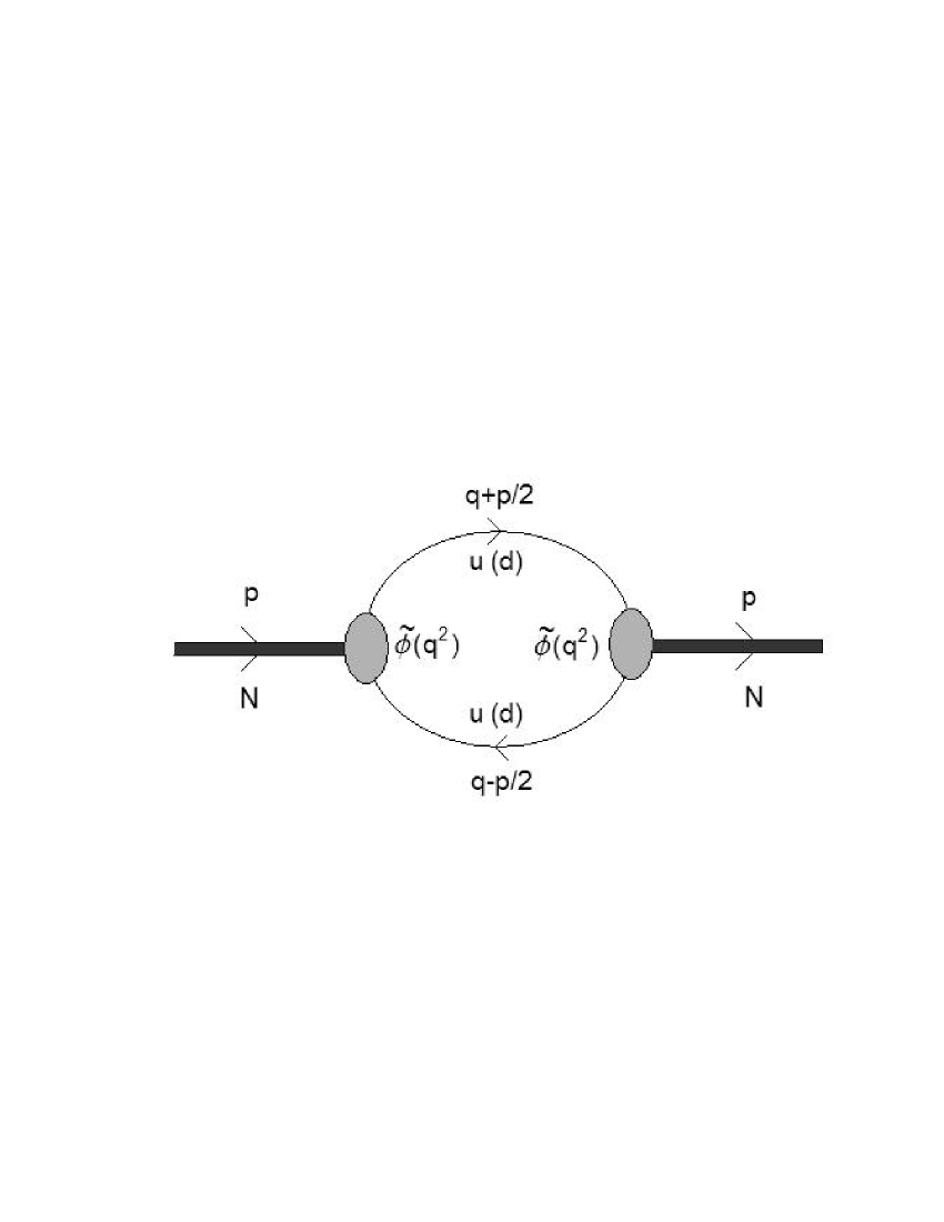
FIG. 1.: N-meson mass operator diagram.

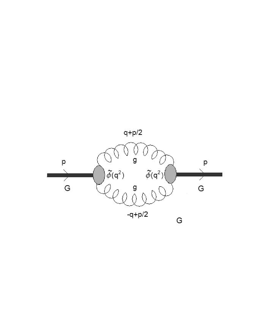
FIG. 2.: Glueball mass operator diagam.

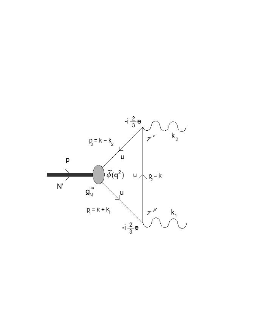
FIG. 3.: $N^{\prime}\equiv f_{0}(1370)$ meson decaying into two photons through a u-loop.

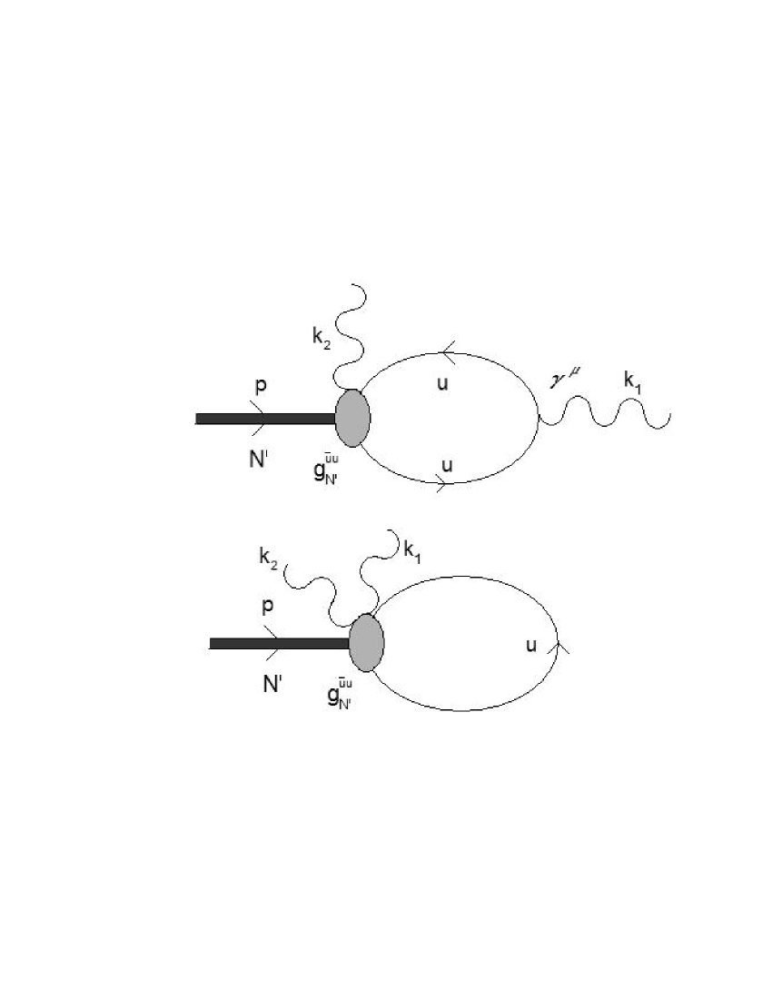
FIG. 4.: Bubble and tadpole diagrams for the two-photon decay of the $N^{\prime}\equiv f_{0}(1370)$ meson. Both diagrams are suppressed, but conceptually important for conservation of gauge invariance.

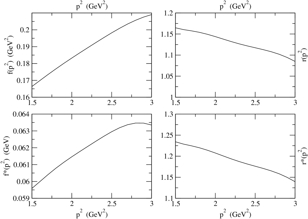
FIG. 5.: Plot of the mixing functions $f(p^{2}),r(p^{2})$ (eq. (52)) and $f^{*}(p^{2}),r^{*}(p^{2})$ (eq. (60)) for the first propagator choice and with a vertex cut-off $\Lambda=1.5$ $GeV.$

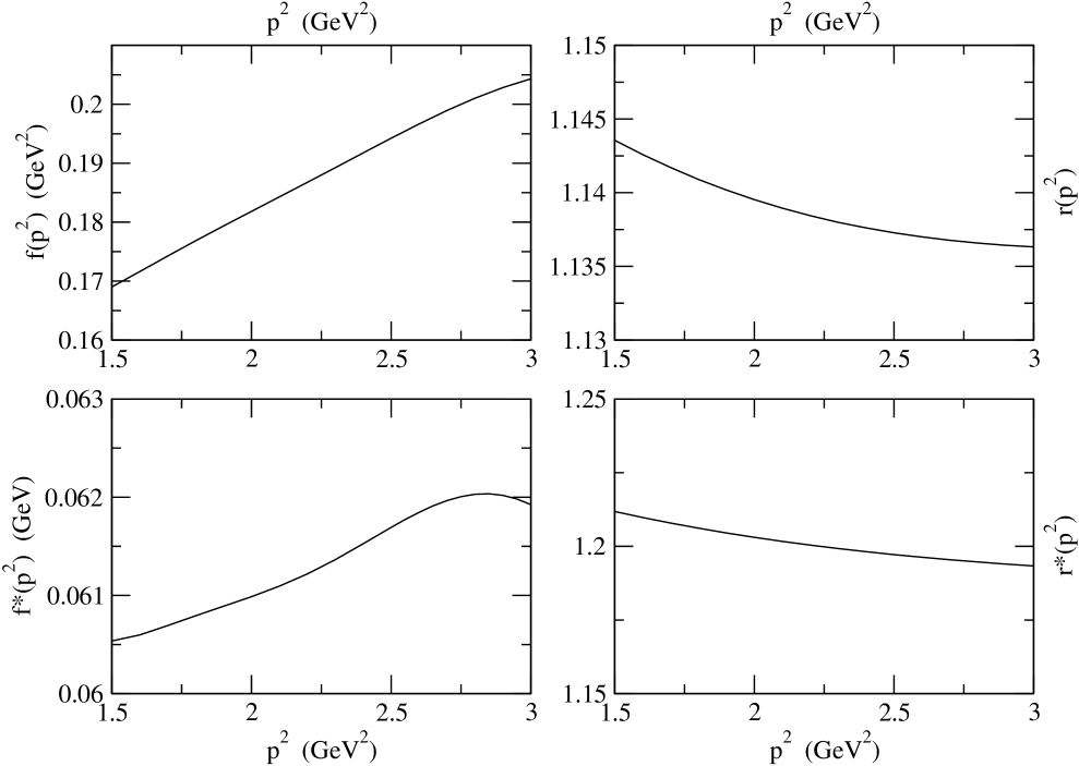
FIG. 6.: Plot of the mixing functions $f(p^{2}),r(p^{2})$ (eq. (52)) and $f^{*}(p^{2}),r^{*}(p^{2})$ (eq. (60)) for the second propagator choice and with a vertex cut-off $\Lambda=1.5$ $GeV.$

REFERENCES

- [1] C. Amsler and F. E. Close, Phys. Lett. B 353, 385 (1995) [arXiv:hep-ph/9505219]. C. Amsler and F. E. Close, Phys. Rev. D 53, 295 (1996) [arXiv:hep-ph/9507326].
- [2] C. Amsler, Rev. Mod. Phys. 70, 1293 (1998) [arXiv:hep-ex/9708025].
- [3] R. Bellazzini et al. [GAMS Collaboration], Phys. Lett. B 467, 296 (1999).
- [4] D. V. Bugg, I. Scott, B. S. Zou, V. V. Anisovich, A. V. Sarantsev, T. H. Burnett and S. Sutlief, Phys. Lett. B 353, 378 (1995).
- [5] R. Barate et al. [ALEPH Collaboration], Phys. Lett. B 472, 189 (2000) [arXiv:hep-ex/9911022].
- [6] C. Michael, arXiv:hep-lat/0302001.
- [7] M. Strohmeier-Presicek, T. Gutsche, R. Vinh Mau and A. Faessler, Phys. Rev. D 60, 054010 (1999) [arXiv:hep-ph/9904461].
- [8] W. J. Lee and D. Weingarten, Phys. Rev. D 61, 014015 (2000) [arXiv:hep-lat/9910008]. D. Weingarten, Nucl. Phys. Proc. Suppl. 53, 232 (1997) [arXiv:hep-lat/9608070].
- [9] F. E. Close and A. Kirk, Eur. Phys. J. C 21, 531 (2001) [arXiv:hep-ph/0103173].
- [10] F. E. Close and N. A. Tornqvist, J. Phys. G 28, R249 (2002) [arXiv:hep-ph/0204205].
- [11] P. Minkowski and W. Ochs, Eur. Phys. J. C 9, 283 (1999) [arXiv:hep-ph/9811518].
- [12] V. V. Anisovich, V. A. Nikonov and A. V. Sarantsev, Phys. Atom. Nucl. 66, 741 (2003) [Yad. Fiz. 66, 772 (2003)] [arXiv:hep-ph/0108188].
- [13] H. G. Dosch and S. Narison, arXiv:hep-ph/0208271.
- [14] C. Amsler and N. A. Tornqvist, Phys. Rept. 389, 61 (2004).
- [15] E. Klempt, arXiv:hep-ex/0101031.
- [16] M. Jaminon and B. van den Bossche, Nucl. Phys. A 636, 113 (1998) [arXiv:nucl-th/9712029].
- [17] D. Ebert, M. Nagy, M. K. Volkov and V. L. Yudichev, Eur. Phys. J. A 8, 567 (2000) [arXiv:hep-ph/0007131].
- [18] M. K. Volkov and V. L. Yudichev, Eur. Phys. J. A 10, 223 (2001) [arXiv:hep-ph/0103003].
- [19] T. Hatsuda and T. Kunihiro, Phys. Rept. 247, 221 (1994) [arXiv:hep-ph/9401310].
- [20] S. P. Klevansky, Rev. Mod. Phys. 64, 649 (1992).
- [21] U. Vogl and W. Weise, Prog. Part. Nucl. Phys. 27, 195 (1991).
- [22] A. Faessler, T. Gutsche, M. A. Ivanov, V. E. Lyubovitskij and P. Wang, Phys. Rev. D 68, 014011 (2003) [arXiv:hep-ph/0304031].
- [23] M. A. Ivanov, M. P. Locher and V. E. Lyubovitskij, Few Body Syst. 21, 131 (1996) [arXiv:hep-ph/9602372].
- [24] I. V. Anikin, M. A. Ivanov, N. B. Kulimanova and V. E. Lyubovitskij, Z. Phys. C 65, 681 (1995).
- [25] M. A. Ivanov, J. G. Korner, V. E. Lyubovitskij and A. G. Rusetsky, Phys. Rev. D 60, 094002 (1999) [arXiv:hep-ph/9904421].
- [26] R. Alkofer and L. von Smekal, Phys. Rept. 353, 281 (2001) [arXiv:hep-ph/0007355].
- [27] D. Ebert, T. Feldmann and H. Reinhardt, Phys. Lett. B 388, 154 (1996) [arXiv:hep-ph/9608223].
- [28] S. Ahlig, R. Alkofer, C. S. Fischer, M. Oettel, H. Reinhardt and H. Weigel, Phys. Rev. D 64, 014004 (2001) [arXiv:hep-ph/0012282].
- [29] R. Alkofer, P. Watson and H. Weigel, Phys. Rev. D 65, 094026 (2002) [arXiv:hep-ph/0202053].
- [30] A. Salam, Nuovo Cim. 25, 224 (1962). S. Weinberg, Phys. Rev. 130, 776 (1963).
- [31] G. V. Efimov and M. A. Ivanov,“The Quark Confinement Model of Hadrons,”, IOP Publishing, Bristol&Philadelfia, 1993.
- [32] Y. A. Simonov, Phys. Atom. Nucl. 64, 1876 (2001) [Yad. Fiz. 64, 1959 (2001)] [arXiv:hep-ph/0110033].
- [33] Y. A. Simonov, arXiv:hep-ph/9911237.
- [34] J. E. Mandula, Phys. Rept. 315 (1999) 273.
- [35] M. A. Ivanov and R. K. Muradov, JETP Lett. 42, 367 (1985).
- [36] A. B. Kaidalov and Y. A. Simonov, Phys. Atom. Nucl. 63, 1428 (2000) [Yad. Fiz. 63, 1428 (2000)] [arXiv:hep-ph/9911291].
- [37] D. Dudal, H. Verschelde, J. A. Gracey, V. E. R. Lemes, M. S. Sarandy, R. F. Sobreiro and S. P. Sorella, JHEP 0401, 044 (2004) [arXiv:hep-th/0311194].
- [38] W. J. Lee and D. Weingarten, arXiv:hep-lat/9805029.
- [39] G. S. Bali, K. Schilling, A. Hulsebos, A. C. Irving, C. Michael and P. W. Stephenson [UKQCD Collaboration], Phys. Lett. B 309, 378 (1993) [arXiv:hep-lat/9304012]. G. S. Bali et al. [TXL Collaboration], Phys. Rev. D 62, 054503 (2000) [arXiv:hep-lat/0003012].
- [40] C. Morningstar and M. J. Peardon, AIP Conf. Proc. 688, 220 (2004) [arXiv:nucl-th/0309068].
- [41] A. A. Natale, Mod. Phys. Lett. A 14, 2049 (1999) [arXiv:hep-ph/9909347].
- [42] K. Langfeld, H. Reinhardt and J. Gattnar, Nucl. Phys. B 621, 131 (2002) [arXiv:hep-ph/0107141].
- [43] K. I. Kondo, arXiv:hep-th/0307270.
- [44] K. Amemiya and H. Suganuma, Phys. Rev. D 60, 114509 (1999) [arXiv:hep-lat/9811035].
- [45] D. Dudal, A. R. Fazio, V. E. R. Lemes, M. Picariello, M. S. Sarandy, S. P. Sorella and H. Verschelde, Nucl. Phys. Proc. Suppl. 127C, 154 (2004) [arXiv:hep-th/0304249].
- [46] E. Gubankova, C. R. Ji and S. R. Cotanch, Phys. Rev. D 62, 074001 (2000) [arXiv:hep-ph/0003289].
- [47] F. Kleefeld, E. van Beveren, G. Rupp and M. D. Scadron, Phys. Rev. D 66, 034007 (2002) [arXiv:hep-ph/0109158].
- [48] M. A. DeWitt, H. M. Choi and C. R. Ji, Phys. Rev. D 68, 054026 (2003) [arXiv:hep-ph/0306060].
- [49] J. Terning, Phys. Rev. D 44, 887 (1991).
- [50] K. Hagiwara et al. [Particle Data Group Collaboration], Phys. Rev. D 66, 010001 (2002).
- [51] D. E. Groom et al. [Particle Data Group Collaboration], Eur. Phys. J. C 15, 1 (2000).
- [52] S. Eidelman et al. [Particle Data Group Collaboration], Phys. Lett. B 592, 1 (2004).