KWIECIŃSKI-CCFM
UNINTEGRATED PARTON DISTRIBUTIONS -
A FEW APPLICATIONS

Abstract

A few applications of recent unintegrated parton distributions from the solution of the recent equations formulated by Jan Kwieciński are shown.

1 Introduction

This talk shortly reviews practical applications of the unintegrated parton distributions which fulfil the Kwieciński evolution equations [1, 2, 3, 4]. The formal aspect is discussed in a parallel talk by Broniowski. I present some examples of application of the formalism. This talk is based on Refs.[7, 9, 14] where more details can be found.

2 Production of gauge bosons

In the formalism of unintegrated parton distributions the nonzero transverse momenta of gauge bosons are obtained already in the leading order. The invariant cross section for inclusive gauge boson production reads then as

$$\frac{d\sigma}{dyd^{2}p_{t,W}}=\sigma_{0}^{W}\sum_{qq^{\prime}}|V_{qq^{\prime}}|^{2}\int\frac{d^{2}\kappa_{1}}{\pi}\frac{d^{2}\kappa_{2}}{\pi}\;\delta^{2}(\vec{p}_{t}-\vec{\kappa}_{1}-\vec{\kappa}_{2})$$

$$\left[f_{q/1}(x_{1},\kappa_{1}^{2},\mu^{2})f_{{\bar{q}^{\prime}}/2}(x_{2},\kappa_{2}^{2},\mu^{2})+f_{{\bar{q}^{\prime}}/1}(x_{1},\kappa_{1}^{2},\mu^{2})f_{q/2}(x_{2},\kappa_{2}^{2},\mu^{2})\right]\;.$$ (1)

In the equation above the delta function assures the conservation of transverse momenta in the $q\bar{q}^{\prime}$ fusion subprocess. The momentum fractions are calculated as $x_{1,2}=\frac{m_{t,W}}{\sqrt{s}}\exp(\pm y)$, where in contrast to the collinear case $M_{W}$ is replaced by the transverse mass $m_{t,W}$.

Introducing unintegrated parton distributions in the space conjugated to the transverse momenta [1]

$$f_{q}(x,\kappa^{2},\mu^{2})=\frac{1}{2\pi}\int\exp\left(i\vec{\kappa}\vec{b}\right)\;\tilde{f}_{q}(x,b,\mu^{2})\;d^{2}b\;,$$ (2)

and taking the exponential representation of the $\delta$ function [7] the formula (1) can be written in the equivalent way

$$\frac{d\sigma}{dyd^{2}p_{t,W}}=\sigma_{0}^{W}/\pi^{2}\sum_{qq^{\prime}}|V_{qq^{\prime}}|^{2}\int d^{2}b\;J_{0}(p_{t}b)$$

$$\left[\tilde{f}_{q/1}(x_{1},b,\mu^{2})\tilde{f}_{{\bar{q}^{\prime}}/2}(x_{2},b,\mu^{2})+\tilde{f}_{{\bar{q}^{\prime}}/1}(x_{1},b,\mu^{2})\tilde{f}_{q/2}(x_{2},b,\mu^{2})\right]\;.$$ (3)

In the formulae for $Z^{0}$ boson production $|V_{qq^{\prime}}|^{2}$ is replaced by $\delta_{qq^{\prime}}\frac{1}{2}(V_{q}^{2}+A_{q}^{2})$.

As already mentioned in the introduction, it is our intention here to use uPDFs $\tilde{f}_{q}^{CCFM}(x,b,\mu^{2})$ which fulfil b-space CCFM equations [1, 2]. However, the perturbative solutions $\tilde{f}_{q}^{CCFM}(x,b,\mu^{2})$ do not include nonperturbative effects such as, for instance, intrinsic momentum distribution of partons in colliding hadrons. In order to include such effects we propose to modify the perturbative solution $\tilde{f}_{q}^{CCFM}(x,b,\mu^{2})$ and write the modified parton distributions $\tilde{f}_{q}(x,b,\mu^{2})$ in the simple factorized form

$$\tilde{f}_{q}(x,b,\mu^{2})=\tilde{f}_{q}^{CCFM}(x,b,\mu^{2})\cdot F_{q}^{NP}(b)\;.$$ (4)

In the present study we shall use two different functional forms for the form factor

$$F_{q}^{NP}(b)=F^{NP}(b)=\exp\left(-\frac{b^{2}}{4b_{0}^{2}}\right)\;or\;\exp\left(-\frac{b}{b_{e}}\right)$$ (5)

identical for all species of partons. In Eq.(5) $b_{0}$ (or $b_{e}$) is the only free parameter. In the next section we try to adjust this parameter to the experimental data on transverse momentum distribution of $W^{\pm}$.

Figure 1: Transverse momentum distribution of $W^{+}+W^{-}$ at W = 1.8 TeV within the formalism of the CCFM uPDF’s with Gaussian (left panel) and exponential (right panel) form factor. The three curves correspond to different values of the form factor parameter $b_{0}$ or $b_{e}$ as explained in the text. The experimental data are taken from Ref.[8].

As an example in Fig.1 we show transverse momentum distribution (integrated over rapidities) of $W^{\pm}$ in proton-antiproton collissions at Fermilab at W = 1.8 TeV for Gaussian (left panel) and exponential (right panel) form factor. The three curves in the left panel show results obtained with different values of the Gaussian form factor parameter $b_{0}$: $b_{0}$ = 0.5 GeV^-1 (dashed), $b_{0}$ = 1.0 GeV^-1 (solid) and $b_{0}$ = 2.0 GeV^-1 (dotted). Similarly, the curves in the right panel correspond to $b_{e}$ = 0.5 GeV^-1 (dashed), $b_{e}$ = 1.0 GeV^-1 (solid) and $b_{e}$ = 2.0 GeV^-1 (dotted). The results are overimposed on the D0 collaboration data [8] measured at Fermilab. The figure clearly demonstrates the importance of the nonperturbative effects. A better agreement is obtained with the exponential form factor. In Ref.[7] the results of the uPDF approach are compared with the results of the standard resummation approach.

3 Charm-anticharm correlations

The total cross section for quark-antiquark production in the reaction $\gamma+p\to Q+\bar{Q}+X$ can be written as

$$\sigma^{\gamma p\to Q\bar{Q}}(W)=\int d\phi\int dp_{1,t}^{2}\int dp_{2,t}^{2}\int dz\;\frac{f_{g}(x_{g},\kappa^{2})}{\kappa^{4}}\cdot\tilde{\sigma}(W,\vec{p}_{1,t},\vec{p}_{2,t},z)\;.$$ (6)

In the formula above $f_{g}(x,\kappa^{2})$ is the unintegrated gluon distribution. The gluon transverse momentum is related to the quark/antiquark transverse momenta $\vec{p}_{1,t}$ and $\vec{p}_{2,t}$ as:

$$\kappa^{2}=p_{1,t}^{2}+p_{2,t}^{2}+2p_{1,t}p_{2,t}cos\phi\;.$$ (7)

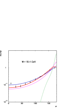
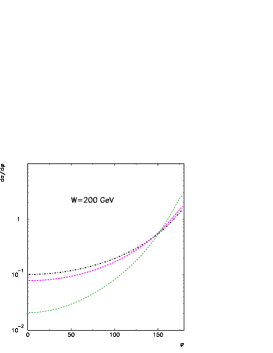
Figure 2: Azimuthal correlations between $c$ and $\bar{c}$. The theoretical results are compared to the recent results from [10] (fully reconstructed pairs).

The azimuthal correlation functions $w(\phi)$ defined as:

$$w(\phi)=\int dp_{1,t}^{2}\int dp_{2,t}^{2}\int dz\;\frac{f_{g}(x_{g},\kappa^{2})}{\kappa^{4}}\cdot\tilde{\sigma}(W,\vec{p}_{1,t},\vec{p}_{2,t},z)\;.$$ (8)

and normalized to unity for two energies of $W$ = 18.4 GeV (FOCUS) and $W$ = 200 GeV (HERA) are shown in Fig.2. The GBW-glue (thin dashed) gives too strong back-to-back correlations for the lower energy. Another saturation model (KL, [11]) provides more angular decorrelation, in better agreement with the experimental data. The BFKL-glue (dash-dotted) provides very good description of the data. The same is true for the CCFM-glue (thick solid) and resummation-glue (thin solid). The latter two models are more adequate for the lower energy. In the present calculations we have used exponential form factor with $b_{e}$ = 0.5 GeV^-1 (see [7]). For comparison in panel (b) we present predictions for $W$ = 200 GeV. Except of the GBW model, there is only a small increase of decorrelation when going from the lower fixed-order energy region to the higher collider-energy region.

4 Production of pions in NN collisions

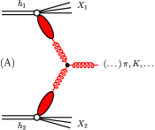
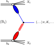
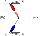
Figure 3: Leading-order diagrams for parton production

The $gg\to g$ mechanism considered in the literature is not the only one possible. In Fig.3 we show two other LO diagrams. They are potentially important in the so-called fragmentation region. The formulae for inclusive quark/antiquark distributions are similar to formula for gluons and will be given explicitly elsewhere [14]. The inclusive distributions of hadrons (pions, kaons, etc.) are obtained through a convolution of inclusive distributions of partons and flavour-dependent fragmentation functions

$$\frac{d\sigma(\eta_{h},p_{t,h})}{d\eta_{h}d^{2}p_{t,h}}=\int_{z_{min}}^{z_{max}}dz\frac{J^{2}}{z^{2}}$$

$$D_{g\rightarrow h}(z,\mu_{D}^{2})\frac{d\sigma_{gg\to g}^{A}(y_{g},p_{t,g})}{dy_{g}d^{2}p_{t,g}}\Bigg{|}_{y_{g}=\eta_{h}\atop p_{t,g}=Jp_{t,h}/z}$$

$$\sum_{f=-3}^{3}D_{q_{f}\rightarrow h}(z,\mu_{D}^{2})\frac{d\sigma_{q_{f}g\to q_{f}}^{B_{1}}(y_{q_{f}},p_{t,q_{f}})}{dy_{q_{f}}d^{2}p_{t,q}}\Bigg{|}_{y_{q}=\eta_{h}\atop p_{t,q}=Jp_{t,h}/z}$$

$$\sum_{f=-3}^{3}D_{q_{f}\rightarrow h}(z,\mu_{D}^{2})\frac{d\sigma_{gq_{f}\to q_{f}}^{B_{2}}(y_{q_{f}},p_{t,q_{f}})}{dy_{q_{f}}d^{2}p_{t,q}}\Bigg{|}_{y_{q}=\eta_{h}\atop p_{t,q}=Jp_{t,h}/z}\;.$$

In Fig.4 we show the distribution in pseudorapidity of charged pions calculated with the help of the CCFM parton distributions [3] and the Gaussian form factor (5) with $b_{0}$ = 0.5 GeV^-1, adjusted to roughly describe the UA5 collaboration data. Now both gluon-gluon and (anti)quark-gluon and gluon-(anti)quark fussion processes can be included in one consistent framework.

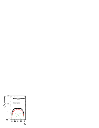
Figure 4: Pseudorapidity distribution of charged pions at W = 200 GeV calculated with the CCFM parton distributions. The experimental data are taken from [13]. The thin solid line is the gluon-gluon contribution while the dashed lines represent the gluon-(anti)quark and (anti)quark-gluon contributions.

As anticipated the missing up to now terms are more important in the fragmentation region, although its contribution in the central rapidity region is not negligible. More details concerning the calculation will be presented elsewhere [14].

For completeness in Fig.5 we show transverse momentum distribution of positive and negative pions for different incident energies. The presence of diagrams $B_{1}$ and $B_{2}$ leads to an asymmetry in $\pi^{+}$ and $\pi^{-}$ production. The higher the incident energy the smaller the asymmetry. This is caused by the dominance of diagram $A$ at high energies.

Figure 5: Transverse momentum distribution of $\pi^{+}$ (solid) and $\pi^{-}$ (dashed) mesons in proton-proton collisions for different center-of-mass energies.

5 Summary

I have presented three examples of application of unintegrated parton distributions to the description of three different processes. Adjusting a value of one parameter of the nonperturbative form factor a good description of different experimental data is achieved. The uPDF which fulfil the Kwieciński equations give a better description of the intermediate-x data than other unintegrated distributions in the literature. Many more additional tests are possible and will be done in the future.

References

• [1] J. Kwieciński, Acta Phys. Polon. B33 (2002) 1809.
• [2] A. Gawron and J. Kwieciński, Acta Phys. Polon. B34 (2003) 133.
• [3] A. Gawron, J. Kwieciński and W. Broniowski, Phys. Rev. D68 (2003) 054001.
• [4] A. Gawron and J. Kwieciński, hep-ph/0309303.
• [5] W. Broniowski, these proceedings.
• [6] A. Szczurek and M. Łuszczak, these proceedings.
• [7] J. Kwieciński and A. Szczurek, Nucl. Phys. B680 (2004) 164.
• [8] V.M. Abazov et al. (D0 collaboration), Phys. Lett. B517 (2001) 299.
• [9] M. Łuszczak and A. Szczurek, Phys. Lett. B594 (2004) 291.
• [10] J.M. Link et al. (FOCUS collaboration), Phys. Lett. B566 (2003) 51.
• [11] D. Kharzeev and E. Levin, Phys. Lett. B523 (2001) 79.
• [12] A. Szczurek, Acta Phys. Polon. 34 (2003) 3191.
• [13] G.J. Alner et al. (UA5 collaboration), Z. Phys. C33 (1986) 1.
• [14] A. Szczurek and M. Czech, a paper in preparation.