NDA and perturbativity in Higgsless models

Michele Papucci

Scuola Normale Superiore and INFN, Piazza dei Cavalieri 7, I-56126 Pisa, Italy

1 Introduction

Models where Electroweak Symmetry Breaking (EWSB) is triggered by boundary conditions for the gauge fields along a compact extra dimension have been proposed during the last year [1, 2, 3]. In 4D if the Higgs is removed from the Standard Model (SM), the scattering amplitudes of the longitudinally polarized vector bosons grow quadratically with the energy and rapidly violate unitarity bounds. Similarly, in these five dimensional models there is no Higgs boson, but here unitarity of scattering amplitudes is recovered by the presence of Kaluza Klein (KK) replicas of gauge bosons [1, 4]. Further investigations have shown the similarities between these models and Technicolor (TC) models in 4D where the Electroweak Symmetry is dynamically broken by some kind of strong interacting physics [2, 3, 5]. In particular, this connection is transparent in warped models using the AdS/CFT duality. Here the 5D KK states correspond to resonances of the strong sector of the TC-like dual 4D theory. Moreover, some of the results retrieved in warped models using the duality remain also valid in general metrics. Differently to standard TC models, in 5D Higgsless theories the first “resonances” can appear in an energy range where the theory is still perturbative. In this case calculability is clearly improved. Moreover early Naive Dimensional Analysis (NDA) [6] estimates of the perturbativity range indicated a cutoff lying in the 10 TeV region, parametrically higher than the one in 4D Higgsless models.

This has mainly motivated the interest in Higgsless theories as a novel possibility in addressing the EWSB problem. A deeper analysis has shown that they share with TC models the production of large corrections to Electroweak Precision observables. The effects are already large in the pure gauge sector and get worse when matter is taken into account [3, 7, 8, 9, 10]. Modifications have been introduced to try to reconcile them with precision data [11]. At present it seems impossible to succeed in this task, and this kind of theories are almost ruled out by past experiments [12].

Yet, it remains interesting to analyze how well qualitative expectations are respected in these models. In fact, the results coming from NDA estimates can also be useful in a more general context and they are usable in other situations where a gauge symmetry is broken by boundary conditions.

Naive dimensional analysis (NDA) is a powerful tool to estimate coefficients of operators in various dimensions taking into account loops and geometrical factors [13]. However, as it is stressed by its name, NDA is naive, since it does not account for order one factors. These are sometimes numerically as big as the “geometrical” $\pi$ factors meaningfully taken into account. In the following we want to test with an explicit calculation how robust some quantitative conclusions derived by NDA can be. In particular we are interested in the cutoff of a 5D Higgsless model as well as in its relation with the one of the correspondent 4D theory. The method used in the explicit determination of the cutoff is the analysis of tree level unitarity in gauge vector bosons scatterings.

In Sect. 2 we recall the NDA results of the 5D cutoff of a Higgsless theory. In Sect. 3 we set up the playground for the explicit calculation of the $WW\rightarrow WW$ scattering amplitudes, both elastic and inelastic. In Sect. 4 we define the analysis of tree level unitarity using elicity amplitudes. The results of the unitarity cutoff are then presented in Sect. 5 and compared with NDA estimates, while conclusions are drawn in Sect. 6.

2 NDA estimation of the cutoff

It is well known that a 4D Yang-Mills theory, in which the gauge symmetry is broken by some kind of strongly interacting physics, becomes strongly coupled at energies of the order of $4\pi v$ where $v$ is the symmetry breaking scale. In terms of $v$ the mass of the gauge bosons is given, as usual, by $M=gv/\sqrt{2}$ where $g$ is the coupling constant. This implies $\Lambda_{4}=4\sqrt{2}\pi M/g$. Thus in the case of the usual 4D SM without the Higgs boson the cutoff is $\Lambda_{4}\simeq 2TeV$.

We are interested in comparing this result with the Higgsless model one. Therefore it is necessary to repeat the NDA estimate in a 5D Yang-Mills theory broken by boundary conditions on an orbifold.

Let’s start recalling the well-known result of NDA applied to a 5D Yang-Mills theory in a non-compact space

$$\Lambda_{5}=24\pi^{3}/g_{5}^{2}$$ (1)

where $g_{5}$ is the 5D gauge coupling whose dimension is (mass)^1/2. This result remains unchanged if we compactify the fifth dimension on a circle, because the UV cutoff is essentially determined by local physics and this kind of compactification does not introduce any modification at short distances. The only requirement is for the whole picture to make sense, i.e. the new scale $1/R$, introduced by the compactification, has to be lower than the cutoff (1). Things are different if we compactify the theory on an orbifold, or more generically on a segment, since here the physics can be different whether it is probed near one of the fixed points or far from them. Orbifold projections change UV physics and in general new terms introduced at the fixed points can change eq. (1).

Let us now specialize to Higgsless models. In a five dimensional theory of EWSB without a Higgs, one requires only the photon to be a massless particle, while the other vector bosons and adjoint scalars (5-th components of vector fields) to be massive. We formulate the theory on a segment and these requirements fix the boundary conditions (BC) for all the fields. It is possible to use gauge freedom and go in unitary gauge reabsorbing massive adjoint scalars and leaving only massive vector bosons. At this point, if one does not add any new interaction at the fixed points and repeat NDA analysis in this configuration, one finds that eq. (1) is still valid. An equivalent procedure consists in adding boundary localized mass terms to the vector bosons. In the limit $m\rightarrow\infty$ one would get the same results as imposing BC. In this alternative setup one can consider these mass terms as originating by non-linear sigma models in the limit $f\rightarrow\infty$ [3]. Using a Feynmann-’t Hooft gauge where localized Goldstone bosons and adjoint scalars are explicitly present, the validity of (1) could be easily checked. Moreover a direct check will be provided by the explicit determination of the unitarity cutoff shown below. With this approach it can also be shown that the absence of any massless scalar is not maintained if we add mass terms localized at both the boundaries. In fact one can use gauge freedom to eliminate Goldstone bosons from one of the non linear sigma models localized at the boundaries, but the Goldstones at the other boundary will be present in the spectrum, as it is also clear from its deconstructed version.

Let us now return to the NDA estimate (1). To compare it with what NDA says on the cutoff of a standard 4D TC, one has to plug in (1) the relation between $g_{5}$ and the effective 4D coupling $g$, and express the W mass in terms of $R$.

The relation between $g_{5}$ and $g$ can be obtained integrating along the compact dimension the $W$-boson wave-functions (which are not flat since the $W$’s are massive). To do this one can either use the cubic or the quartic vertex. Using the 4W vertex for the determination, it is easy to see that in the previous setup one has

$$g_{4} =\frac{g_{5}}{\sqrt{2\pi R}}\sqrt{\frac{3}{2}}$$ (2)

$$M =\frac{1}{2R}$$ (3)

which gives

$$\Lambda_{5}=\frac{9\pi}{g\sqrt{2}}\Lambda_{4}$$ (4)

This analysis suggests that the cutoff of a 5D Higgsless theory is higher by a factor $k\pi/g$ with respect to the 4D one with the same mass and coupling. To better understand the origin of this increase it is useful to introduce the parameter $N\equiv\Lambda_{5}R$, which in flat geometries is related to the number of KK states below the cutoff. One can then rewrite the previous equations in terms of $N$ and of $\Delta M_{KK}$, the mass splitting between 2 KK gauge bosons. We get

$$g_{5} =2\pi\sqrt{\frac{6\pi}{N\Delta M_{KK}}}$$ (5)

$$\Lambda_{5} =N\Delta M_{KK}$$ (6)

$$\Lambda_{4} =\frac{2}{3}\sqrt{N}\Delta M_{KK}$$ (7)

$$\Lambda_{5}/\Lambda_{4} =\frac{3}{2}\sqrt{N}$$ (8)

From eq. (8) we can see that the before-mentioned increment is due to the presence of the additional KK states below the cutoff. They remedy for the bad energy behavior of the amplitudes and postpone unitarity violation. Therefore the effect is proportional to $\sqrt{N}$.

However this analysis is naive and order 1 factor in the coefficients of the previous expressions can numerically modify the results, potentially reabsorbing the increment, especially when $N$ is not very large.

Moreover these are the results for the simplest 5D theory, with equally spaced KK states. Unfortunately it is not phenomenologically interesting, because the spacing is $1/R\equiv 2M_{W}$, too small to be in accordance with the experiments.

It is therefore necessary to create a bigger separation between the lowest states and the heavier ones. Furthermore one has to make the excited states of vector bosons less coupled to the low energy theory in the hope to reconcile the model with the EWPT. This can be achieved either by progressively increasing the size of the coefficient of boundary localized kinetic terms for gauge fields [3] or by using a warped background [2]. From now on we will follow Ref. [3] and focus on the case of a flat background with a brane-localized kinetic operator.

This term introduces a new parameter in the cutoff relation and in principle can modify or even lower the cutoff.

NDA still suggests that, apart from ${\cal O}(1)$ factors, this is not the case and that in this kind of setup such a localized kinetic term does not modify the qualitative behavior of the cutoff.

A way to see this fact would be to repeat NDA in a different gauge as indicated in [14]. It is sufficient to see that the UV behavior of Goldstones and adjoint scalars’ propagators is not changed by the localized kinetic term. NDA goes like in the standard bulk case and eq. (1) remains unchanged.

Thus the main effects of a kinetic term are the change in the relation between the 4D and the 5D coupling constant and in the relation between $M_{W}$ and the 5D parameters $g$, $g_{5}$ and $L=\pi R$. The relation between $\Lambda_{5}$, $\Lambda_{4}$ and $N$ are changed consequently. The relevant equations, when $g^{2}L/g_{5}^{2}$ is small, are

$$g_{4}\simeq g(1-\frac{g^{2}L}{4g_{5}^{2}})$$ (9)

$$M\simeq\frac{g}{g_{5}\sqrt{L}}(1-\frac{g^{2}L}{6g_{5}^{2}})$$ (10)

$$\Lambda_{4}\simeq\frac{2}{\sqrt{3}}\frac{\sqrt{N}}{\pi}\Delta M_{KK}(1+\frac{Ng_{4}^{2}}{288\pi^{2}})$$ (11)

$$\Lambda_{5}/\Lambda_{4}\simeq\frac{\sqrt{3}\pi}{2}\sqrt{N}(1-\frac{Ng_{4}^{2}}{288\pi^{2}})$$ (12)

A few words of comment are necessary. Eq. (1) gets corrected when $g^{2}L/g_{5}^{2}$ become very large, i.e. when higher order corrections from localized kinetic terms become important. Trusting $\pi$ factors, NDA suggests that the coefficient of $\sqrt{N}$ in the $\Lambda_{5}/\Lambda_{4}$ ratio is bigger than the one in the pure bulk result by a factor $\pi/\sqrt{3}$. This means that not only the cutoff of a 5D Higgsless theory is parametrically higher than the one in 4D due to the effect of the KK tower, but there is also the possibility to increase this gain by another “geometrical” constant factor by increasing the separation between the low lying state and the higher ones [15]. Since this result can be of phenomenological interest but it is retrieved using NDA estimates and is ${\cal O}(1)$, it needs to be checked whether it may be canceled by other ${\cal O}(1)$ factors not taken into account by NDA.

3 The $WW\rightarrow WW$ scattering

Let us now begin defining the model used in the analysis before and then we will describe the calculation of the $2\rightarrow 2$ scattering for $W$ bosons. The helicity amplitude analysis will be illustrated in the next section.

We consider a 5D gauge theory compactified on a segment $[0,L]$, parameterized by the coordinate $y$. For simplicity we assume the gauge group to be $SU(2)$, completely broken by boundary conditions at $y=L$. This assumption is simple but general enough to apply also to the flat space Higgsless models in the limit $g^{\prime}\rightarrow 0$ [3]. As stated before the gauge breaking can be achieved by adding by hand to the gauge fields a mass term localized at $y=L$.

The relevant Lagrangian is then given by

$${\cal L}={\cal L}_{5}+{\cal L}_{0}\delta(y)+{\cal L}_{L}\delta(y-L)$$ (13)

where

$${\cal L}_{0}= -\frac{1}{4g^{2}}F_{\mu\nu}^{a}F^{\mu\nu\ a}$$ (14)

$${\cal L}_{5}= -\frac{1}{4g_{5}^{2}}F_{MN}^{a}F^{MN\ a}$$ (15)

$${\cal L}_{L}= -m^{2}W_{\mu}^{a}W^{\mu\ a}$$ (16)

where Greek letters indicate 4D coordinates while capital letters the 5D ones, and $a=1,2,3$ is the $SU(2)$ gauge index. Letting $m\rightarrow\infty$ we enforce the conditions $W_{\mu}^{a}=0$ at $y=L$ for every $a$. Moreover one can use the residual 5D gauge freedom to eliminate $W_{5}^{a}$, thus working in unitary gauge.

In order to study tree level unitarity in gauge vector boson scatterings one way to proceed is to expand all the field in KK modes, compute the relevant 4D Feynmann graphs and then sum over the KK towers of intermediate states. This procedure has been followed in advance in [1, 16] where the elastic $2\rightarrow 2$ process has been calculated and in [17] where the results of a numerical evaluation of inelastic amplitudes are presented. We do not pursue this way of calculation here, instead we integrate out the degrees of freedom contained in the bulk and we write down an “effective” Lagrangian at $y=0$, i.e. a generating functional for the $y=0$ fields’ amplitudes. This will be the tool used to calculate the scatterings [3, 14]. This is motivated by economy and physically by the fact that in the simplest Higgsless model setup SM matter couples to gauge bosons at $y=0$.

Let $g_{5}=g/M^{1/2}$. $ML$ then parameterizes the ratio between brane and bulk couplings. The regimes in which the brane dominates over the bulk and vice-versa are given by $ML\ll 1$, $ML\gg 1$ respectively. In order to compute the scattering amplitudes we need the $y=0$ “effective” Lagrangian at second order in $g$. Neglecting just for a while gauge and spacetime indexes, the vector bosons can be expanded perturbatively in $g$ as

$$W=W_{0}(x;y)+W_{1}(x;y)+W_{2}(x;y)+\ldots$$ (17)

where $W_{n}$ is of order ${\cal O}(g^{n})$ and the $W_{n}$s satisfy the conditions

$$W_{0}(x;y=0)\equiv\bar{W}(x),\ \ W_{n}(x;y=0)=0\ {\rm if}\ n>0$$ (18)

Then if we indicate with ${\cal L}_{5}^{(2)}(W,W)$, ${\cal L}_{5}^{(3)}(W,W,W)$, ${\cal L}_{5}^{(4)}(W,W,W,W)$ the quadratic, cubic and quartic part of the bulk Lagrangian respectively, the effective Lagrangian for the bulk contribution can be written as

$${\cal L}_{eff}=\int_{0}^{L}dy \left[{\cal L}_{5}^{(2)}(W_{0},W_{0})+{\cal L}_{5}^{(3)}(W_{0},W_{0},W_{0})+{\cal L}_{5}^{(4)}(W_{0},W_{0},W_{0},W_{0})\right.$$

$$+\left.{\cal L}_{5}^{(2)}(W_{1},W_{1})+{\cal L}_{5}^{(3)}(W_{(1},W_{0},W_{0)})\right]$$ (19)

where the other contributions to the perturbative expansion vanish after partial integration and/or use of the conditions (18), while the round parentheses on $W$ indexes mean symmetrization. Moreover the vector boson fields can be decomposed into transverse and longitudinal (gauge-like) components $W=W^{t}+W^{l}$. At zero-order level they satisfy the 5D homogeneous equation of motion

$$(\partial_{5}^{2}+p^{2})W_{0}^{t} =0$$ (20)

$$\partial_{5}^{2}W_{0}^{l} =0$$ (21)

while at first order level they satisfy the inhomogeneous version of the previous equations where the r.h.s. is $1/2(\delta{\cal L}_{5}^{(3)}/\delta W)(W_{0},W_{0})$. At this point one can see that the two terms in the second line of (3) are not independent among each others because the equations of motion enforce the relation

$$\int_{0}^{L}dy\ {\cal L}_{5}^{(2)}(W_{1},W_{1})=-\frac{1}{2}\int_{0}^{L}dy\ {\cal L}_{5}^{(3)}(W_{(1},W_{0},W_{0)})$$ (22)

Before going on a few comments on the physical meaning of (3) are worthly noticing. The first term describes the correction to the vector boson propagator because the W bosons can leave the $y=0$ brane and propagate in the bulk. The second and third terms include the corrections to the interaction vertices because the interaction point can be far from the brane. The last two terms, instead, describe an effective 4-point interaction originating from a tree level 2-2 scattering mediated by a vector boson exchange taking place entirely in the bulk. This can be clearly seen in eq. (27) below from the explicit form of the effective Lagrangian.

Going to momentum space only for the first four coordinates and solving the equations of motion for the vector bosons one finds

$$W^{t}_{0}(k;y) =\bar{W}^{t}(k)\frac{\sin\left(\sqrt{k^{2}}(L-y)\right)}{\sin\left(\sqrt{k^{2}}L\right)}$$ (23)

$$W^{l}_{0}(k;y) =\bar{W}^{l}(k)\frac{L-y}{L}$$ (24)

$$W^{t}_{1}(k;y) =-\bar{W}^{t}(k)\sin\left(\sqrt{k^{2}}(L-y)\right)\int_{0}^{y}ds\frac{1}{\sin^{2}\left(\sqrt{k^{2}}(L-s)\right)}\int_{s}^{L}dt\sin\left(\sqrt{k^{2}}(L-t)\right)\frac{\delta{\cal L}_{5}^{(3)}}{\delta W^{t}}(k;t)$$ (25)

$$W^{l}_{1}(k;y) =-\bar{W}^{t}(k)(L-y)\int_{0}^{y}ds\frac{1}{(L-s)^{2}}\int_{s}^{L}dt(L-t)\frac{\delta{\cal L}_{5}^{(3)}}{\delta W^{l}}(k;t)$$ (26)

where $(\delta{\cal L}_{5}^{(3)}/\delta W)(k;t)\equiv(\delta{\cal L}_{5}^{(3)}/\delta W)(W_{0}(p;t),W_{0}(q;t))$ and momentum conservation $p+q+k=0$ is enforced. Using these formulae the last two terms in the effective Lagrangian can be rewritten as

$$\int_{0}^{L}dy\left(\frac{\sin\left(\sqrt{k^{2}}L\right)}{\sin\left(\sqrt{k^{2}}(L-y)\right)}\right)^{2}\left[\int_{y}^{L}ds\frac{\delta{\cal L}_{5}^{(3)}}{\delta W^{t}}\left(k;s\right)\right]^{2}+\int_{0}^{L}dy\frac{L^{2}}{(L-y)^{2}}\left[\int_{y}^{L}ds\frac{\delta{\cal L}_{5}^{(3)}}{\delta W^{l}}\left(k;s\right)\right]^{2}$$ (27)

which clearly describes a 2-2 bulk scattering mediated by either a longitudinal vector boson or a transverse one. The propagators for the transverse and longitudinal components are:

$$\langle\bar{W}^{t,a}_{\mu}\bar{W}^{t,b}_{\nu}\rangle(k) =-i\delta^{ab}\left(g_{\mu\nu}-\frac{k_{\mu}k_{\nu}}{k^{2}}\right)\frac{1}{k(k-M\cot(kL))}$$ (28)

$$\langle\bar{W}^{l,a}_{\mu}\bar{W}^{l,b}_{\nu}\rangle(k) =i\delta^{ab}\frac{k_{\mu}k_{\nu}}{k^{2}}\frac{L}{M}$$ (29)

Since the W fields in the effective Lagrangian (3) are a superposition of Kaluza Klein fields of different masses, in order to calculate scattering amplitudes among mass eigenstates one has to apply the standard LSZ procedure on external legs multiplying each of them by $Z^{1/2}$. The last ingredient needed is then the pole residue of the zero-order vector boson propagator calculated at $p^{2}=m^{2}_{i}$, the mass of the i-th KK mode. This can be easily retrieved from eq. (28). For a KK state of mass $m$ it is

$$Z^{1/2}=\sqrt{\frac{2}{1+ML\csc(mL)}}$$ (31)

Having computed the relevant Lagrangian ${\cal L}={\cal L}_{0}+{\cal L}_{eff}$ we are able to calculate the $WW\rightarrow WW$ polarized scattering amplitudes in a straightforward way. In particular all the contractions between polarization vectors and external momenta work like in 4D.

4 Elicity amplitudes analysis of tree level unitarity

In order to investigate tree level unitarity one can decompose scattering amplitudes into elicity amplitudes of definite total angular momentum. In the following we will focus on the $J=0$ amplitude which, for massive spin 1 particles, is a 3 by 3 matrix in elicity space. It involves polarized scatterings of vector bosons of same helicity, i.e. $(0,0)$, $(+,+)$ and $(-,-)$.

It is easily seen that a general inelastic channel consists of five different independent amplitudes, because parity and time-reversal constrain the 3 by 3 matrix. Usually in a 4D Higgsless Yang-Mills theory the $(0,0,0,0)$ scattering amplitude grows linearly with $s$ and dominates upon the other polarized channels which are therefore neglected. In this way one can restrict the analysis to a single entry in elicity space. In the 5D case, this amplitude is better-behaved and grows logarithmically with $s$ [1, 4].

One could suspect that the other four elicity amplitudes could not be neglected anymore. However off diagonal amplitudes are smaller than the elicity-conserving ones. This is quite obvious for the $(+,+,-,-)$ amplitude which is well-known to be equal to 0 in the massless limit because of angular momentum conservation. The suppression can be easily derived also for the $(0,0,\pm,\pm)$ amplitudes taking the high energy limit (in this case the role of the KK tower is crucial, as it is crucial the role of the Higgs boson exchange in the SM case).

This fact keeps the $J=0$ matrix nearly diagonal, letting us to concentrate to the $(0,0)\rightarrow(0,0)$ matrix element, which is slightly bigger, but of the same order, of the other “elicity-conserving” amplitudes. To get a numerical feeling of this statement, Fig. 1 shows the elastic elicity amplitudes as a function of $\sqrt{s}$.

Figure 1: Elastic elicity amplitudes. Solid lines: $(0,0,0,0)$ and $(+,+,+,+)$. Dashed lines: $(0,0,+,+)$ and $(+,+,-,-)$.

As to the isospin indices, the $T_{3}=0$ channel will be analyzed. Indeed it is the fastest growing one because it involves both the $W^{+}W^{-}$ and $W^{0}W^{0}$ initial and final states. This 2 by 2 matrix can be easily diagonalized and the biggest eigenvalue, the $T=0$ one, will be taken in the following discussion on unitarity.

Having get rid of helicity, angular momentum and isospin indices with the previous considerations, an infinite matrix remains whose elements are the scattering amplitudes of different KK modes.

Let us define the transition matrix $T$ for $J=0$ amplitudes in such a way that its elements are

$$t_{\alpha\beta}=\frac{1}{32\pi}\int_{-\pi}^{\pi}d\theta{\cal M}_{\alpha\rightarrow\beta}(s;\cos\theta)$$ (32)

where $\alpha$ and $\beta$ are initial and final states labeled by a couple of KK indices. Unitarity constraints can then be recasted in matrix form as [18]

$$T-T^{\dagger}=-2\,i\ T\,\Phi\,T^{\dagger}$$ (33)

where $\Phi$ is the (diagonal) matrix of phase space contributions

$$\Phi_{\alpha}=\frac{2|p_{\alpha}|}{\sqrt{s}}=\sqrt{1+\frac{(m_{n}^{2}-m_{k}^{2})^{2}}{s^{2}}-2\frac{m_{n}^{2}+m_{k}^{2}}{s}}$$ (34)

where $\alpha=(n,k)$, $s$ is the squared C.M. energy and $|p_{\alpha}|$ is the absolute value of 3-momentum in C.M. frame of the state $\alpha$.

As a reference let us recall that when this matrix collapses to a single element $t$ one can derive the usual bound

$$|t|<1$$ (35)

In principle one should diagonalize the matrix equation in (33) and apply the condition (35) to every eigenvalue. It is however cumbersome to diagonalize the full matrix. A somewhat weaker bound can be derived by focusing on one single element of the l.h.s., i.e. on the row of $T$ with two low-lying KK modes as initial state. These are to be identified with SM vector bosons. Unitarity then implies

$$\Phi_{0,0}\,|t_{0,0}|+\frac{1}{|t_{0,0}|}\sum_{(n,m)\neq(0,0)}\Phi_{n,m}\,|t_{n,m}|^{2}<1$$ (36)

where now $t_{n,m}$ represents the $(0,0)\rightarrow(n,m)$ channel and the sum is performed over all accessible states for a given C.M. energy $\sqrt{s}$.

5 Tree-level unitarity and NDA comparison

In this section the scale of the unitarity cutoff is determined by taking into account both elastic and inelastic channels. Since all partial wave amplitudes singularly considered grow logarithmically with $\sqrt{s}$ [1, 4], the previous estimates of the cutoff based on the elastic amplitude alone [16] are in general not reliable when the excited KK states are not very heavy. In fact it is well known that in extra-dimensional models it is the multiplicity of states, i.e. the increasing number of open channels, that leads to unitarity violation and not the growing with the energy of a single amplitude.

In principle, since the kinetic term at $y=0$ completely breaks 5-momentum and every KK state can interact with all the others, one can estimate to have ${\cal O}(n^{2})$ open channels at C.M. energies of the order of the mass of the n-th Kaluza-Klein. If all the open channels had amplitudes of the same order one could expect a quadratic growth with the energy of at least one of the eigenvalues of $T$, hence a dependence of $\Lambda_{5}$ on $N_{KK}^{2}$ which strongly conflicts with NDA. Clearly this is not the case.

The reason is that all the channels which violates momentum along the 5th coordinate are suppressed.

In fact, all the transition amplitudes associated to them have a suppression factor proportional to the sum of the final particles masses, hence to the sum of the KK indices. Restricting the analysis to the 5th momentum-conserving amplitudes only, $(0,0)\rightarrow(n,n\pm 1)$ and $(0,0)\rightarrow(n,n)$, one obtains a transition matrix whose dimension is ${\cal O}(n)\times{\cal O}(n)$. Its largest eigenvalue then scales at most linearly with the number of accessible KK states, in agreement with NDA. Taking into account all the 5th momentum violating amplitudes, because of their suppression, gives an ${\cal O}(1)$ correction but does not modify qualitatively the energy behavior.

As a numerical example of the above statement Fig. 2 shows the l.h.s. of (36) where either all the amplitudes or only the $(0,0)\rightarrow(n,n)$ are included in the sum. In the same Figure it is also plotted the elastic amplitude alone, showing explicitly that inelastic contributions cannot be neglected. Having clarified this point, all the channels will be taken into account in the following computations.

Figure 2: Comparison between l.h.s. of eq. (36) calculated using all the scattering amplitudes (solid line), the 5th momentum-conserving ones (dashed line) and the elastic amplitude alone (dashed-dotted line) for $\sqrt{ML}=0.3$.

It is interesting to compare the 4D amplitude with the 5D elastic and inelastic ones. This is shown in Fig. 3 for two different values of $ML$.

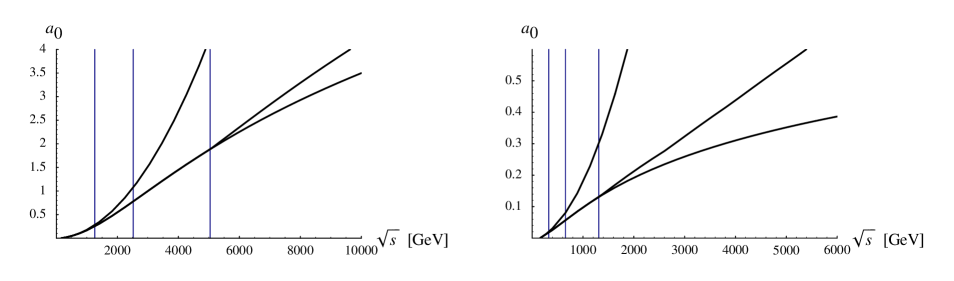
Figure 3: Comparison between 4D, 5D elastic and the l.h.s. of eq. (36) as a function of $\sqrt{s}$. Vertical lines are for $\sqrt{s}=M_{W^{\prime}}/2,M_{W^{\prime}},2M_{W^{\prime}}$. The two figures are plotted for $\sqrt{ML}=0.1,0.4$ respectively.

We can see that the amplitudes in the Higgsless model follow the energy behavior of the 4D one up to energies of the order of $M_{W^{\prime}}/2$, where $W^{\prime}$ is the first excited state. After that the presence of the KK modes modify the quadratic energy dependence into a logarithm. It is also clear that the elastic amplitudes gives the correct behavior up to $2M_{W^{\prime}}$ where the channel into $WW\rightarrow W^{\prime}W^{\prime}$ is open. In this region the energy dependence is almost linear since the $\log(\sqrt{s}/M_{W^{\prime}})$ is small. On the contrary, when the logarithm becomes large, other channels are opened and the elastic amplitude cannot be trusted anymore.

If the KK states are quite heavy then the amplitude becomes large in the region where $\sqrt{s}\lesssim M_{W^{\prime}}$ and it likely saturates the bound before inelastic channels are open. In this case the elastic amplitude suffices in giving a correct estimation of the cutoff. This is also the region where $N_{KK}$ is very small and 5D NDA fails. The cutoff of this 5D Higgsless theory is not too far from the one of a Higgsless SM. Moreover the effective field theory description, which is an expansion series in $1/N_{KK}$, is becoming meaningless when $N_{KK}$ is small. Conversely, if the KK states are light then a full inelastic computation is required. However Figs. 2 and 3 suggest that a behavior linear in energy is early attained and a linear extrapolation using the angular coefficient computed from the elastic amplitude in the range $M_{W^{\prime}}\lesssim\sqrt{s}\lesssim 2M_{W^{\prime}}$ can be a good approximation of the full result.

Let us now return to the comparison of the scattering amplitudes with NDA estimates.

From the perturbative unitarity analysis one can define $\bar{\Lambda}_{5}$ as the energy scale where the bound (36) saturates. Therefore $\bar{\Lambda}_{5}$ can be determined for a given set of values of $M$, $L$ and $g$.

One can compare it with $\Lambda_{5}$ from NDA and check directly both the $24\pi^{3}$ factor in (1) and the dependence of $\Lambda_{5}/\Lambda_{4}$ on $\sqrt{N}$ on (8) and (12).

To check (1) it is convenient to adimensionalize both sides of the equality using $L$. Since the scattering amplitudes are proportional to $g_{5}^{2}/L$, having defined $\bar{N}=\bar{\Lambda}_{5}/\Delta M_{KK}$, the unitarity bound reads

$$g_{5}^{2}/Lf(\bar{N},ML)=1$$ (37)

Inverting this relation, one can easily plot $\bar{N}$ versus $L/g_{5}^{2}$ for different values of the localization parameter $\sqrt{ML}=g\sqrt{L}/g_{5}$.

According to NDA a linear relation with a coefficient $12\pi^{2}$ should be obtained if we identify $N$ with $\bar{N}$. However, as long as eq. (37) is derived from an upper bound on $\Lambda_{5}$, then $\bar{N}\geq N$ and a smaller coefficient suffices.

Figure 4: Solid lines: $\bar{N}$ from eq. (37) as a function of $L/g_{5}^{2}$ for $\sqrt{ML}=0.3,1.75,15$. Dashed lines: the functions $3\pi^{2}L/\sqrt{2}g_{5}^{2}$ and $3\pi^{2}L/g_{5}^{2}$.

Fig. 4 shows $\bar{N}$ as a function of $L/g_{5}^{2}$ for $\sqrt{ML}=0.3,1.75,15$ compared with two linear functions of $\bar{N}$ with different coefficients (dashed lines). As a confirmation of 5D NDA, not only the linear behavior is respected but also the coefficients show the presence of the right power of $\pi$. The difference is only a numerical factor, ranging from $4$ to $4/\sqrt{2}$ as $ML$ changes from $ML\gg 1$ to $ML\ll 1$.

It is now possible to check the NDA result for $\Lambda_{5}/\Lambda_{4}$. Here things are simpler. Any overestimation in the definition of $\bar{\Lambda}$, if in the form of a multiplicative factor, equally affects both $\bar{\Lambda}_{5}$ and $\bar{\Lambda}_{4}$ and cancels out. Since the previous result suggested the presence of such multiplicative factor, we should get a sufficiently reliable result for $\Lambda_{5}/\Lambda_{4}$.

Figure 5: $\Lambda_{5}/\Lambda_{4}\sqrt{N_{KK}}$ as a function of $N_{KK}$ for $\sqrt{ML}=0.05,0.3,1.75,15$.

Here we are interested in the $\sqrt{N}$ coefficient. Hence we focus on the ratio $\bar{\Lambda}_{5}/\bar{\Lambda}_{4}\sqrt{\bar{N}}$, where $\bar{\Lambda}_{5}$ and $\bar{N}$ are defined as before and $\bar{\Lambda}_{4}$ is the unitarity cutoff of the correspondent 4D gauge theory, retrieved using the bound (35). Fig. 5 shows the plot of this quantity versus $\bar{N}$.

One can easily see that the $\sqrt{N}$ dependence of the cutoff ratio is quite good and the that coefficient in eq. (12) is approximately 1 for low values of $ML$ and decreases for higher values of the localization parameter (less localization). This confirms the qualitative NDA result that there is an increment in the ratio between the 5D and 4D cutoffs when a large localized kinetic term is added. It also shows that the numerical values of the $\sqrt{N}$ coefficients in both of the cases are different, lower than the NDA estimates. In particular the increase by $\pi/\sqrt{3}$, as suggested by NDA, is reduced to $1.15$ which is numerically irrelevant.

As a final result one can determine the cutoff for a “realistic” Higgsless theory setting the low lying state at $m_{W}=80\,GeV$ and relating the effective coupling $g_{(0,0,0)}$ between three W bosons to the SM value $g_{SM}$. An additional parameter, $ML$, is left out and can be determined by the position of the first excited state. Fig. 6 shows the results for $\Lambda_{5}$ as a function of $m_{W^{\prime}}$. One can see that the cutoff is always less than about 5 TeV for $m_{W^{\prime}}>500\,GeV$. This result rigorously applies only to the Higgsless “flat” models where the introduction of $g^{\prime}\neq 0$ does not modify the results. However in [19] it is found a numerically similar result also for warped models, although using a stronger bound $Re\,a_{0}<1/2$.

Figure 6: Cutoff of a flat space Higgsless theory as a function of the mass of the first excited vector boson.

This indicates a very low cutoff for those parameters space regions where 5D Higgsless theories are not in disagreement with Electroweak Precision Tests (EWPT) data. In fact EWPT constrain the first resonances exchanged in the neutral channel to be quite heavy, and this lowers the perturbative cutoff. Higher order operators parameterizing UV physics are weighted by powers of $1/N=1/\Lambda R$. Since $N$ turns out to be ${\cal O}(1)$, the price to be paid to be compatible to EWPT is that the same electroweak observables are affected by uncalculable UV physics with potentially large corrections. The situation is not very different from the one in 4D TC, whose calculability these models aimed to improve.

6 Conclusions

In this work we have computed both elastic and inelastic partial waves for 4W scatterings in a 5D Yang-Mills theory broken by boundary conditions. These results allowed us to study how reliable NDA estimates are in a 5D Higgsless theory. In particular, we have explicitly checked the $\sqrt{N}$ dependence of the ratio $\Lambda_{5}/\Lambda_{4}$ between a 5D Higgsless theory and the correspondent 4D one. We have also investigated the enhancement of the coefficient of this relation when a big localized kinetic term is added to the theory. It was found that this increase, suggested by NDA, is reabsorbed by ${\cal O}(1)$ factors which NDA can’t control. Finally we have given a better determination of $\Lambda_{5}$ in 5D Higgsless flat models finding a very low value. $\Lambda_{5}$ can be raised up to about $5\,TeV$ only if $M_{W_{3}^{\prime}}\sim 500\,GeV$, which is however excluded by EWPT. In those parameter space regions where the models are still compatible with EWPT data the cutoff is $2-3\,TeV$, giving $N\sim 2$.

References

- [1] C. Csaki, C. Grojean, H. Murayama, L. Pilo and J. Terning, Phys. Rev. D 69, 055006 (2004) [arXiv:hep-ph/0305237].
- [2] C. Csaki, C. Grojean, L. Pilo and J. Terning, Phys. Rev. Lett. 92, 101802 (2004) [arXiv:hep-ph/0308038].
- [3] R. Barbieri, A. Pomarol and R. Rattazzi, arXiv:hep-ph/0310285.
- [4] R. Sekhar Chivukula, D. A. Dicus and H. J. He, Phys. Lett. B 525, 175 (2002) [arXiv:hep-ph/0111016].
- [5] G. Burdman and Y. Nomura, arXiv:hep-ph/0312247.
- [6] A. Manohar and H. Georgi, Nucl. Phys. B 234 (1984) 189.
- [7] M. E. Peskin and T. Takeuchi, Phys. Rev. Lett. 65, 964 (1990).
- [8] M. Golden and L. Randall, Nucl. Phys. B 361, 3 (1991).
- [9] B. Holdom and J. Terning, Phys. Lett. B 247, 88 (1990).
- [10] C. Csaki, C. Grojean, J. Hubisz, Y. Shirman and J. Terning, arXiv:hep-ph/0310355.
- [11] G. Cacciapaglia, C. Csaki, C. Grojean and J. Terning, arXiv:hep-ph/0401160.
- [12] R. Barbieri, A. Pomarol, R. Rattazzi and A. Strumia, arXiv:hep-ph/0405040.
- [13] Z. Chacko, M. A. Luty and E. Ponton, JHEP 0007, 036 (2000) [arXiv:hep-ph/9909248].
- [14] M. A. Luty, M. Porrati and R. Rattazzi, JHEP 0309 (2003) 029 [arXiv:hep-th/0303116].
- [15] R. Rattazzi, Les Rencontres de Physique de la Vallée d’Aoste, 2004
- [16] R. Foadi, S. Gopalakrishna and C. Schmidt, JHEP 0403 (2004) 042 [arXiv:hep-ph/0312324].
- [17] H. Davoudiasl, J. L. Hewett, B. Lillie and T. G. Rizzo, arXiv:hep-ph/0312193.
- [18] S. De Curtis, D. Dominici and J. R. Pelaez, Phys. Rev. D 67 (2003) 076010 [arXiv:hep-ph/0301059].
- [19] H. Davoudiasl, J. L. Hewett, B. Lillie and T. G. Rizzo, arXiv:hep-ph/0403300.