Implications of the Present Bound on the Width of the $\mathbf{\Theta^{+}(1540)}$

Abstract

The recently reported $\Theta^{+}(1540)$ exotic baryon seems to be very narrow: $\Gamma(\Theta)<$ 1 MeV according to some analyses. Using methods of low energy scattering theory, we develop expectations for the width of the $\Theta$, an elastic resonance in $KN$ scattering in a theory where the characteristic range of interactions is $\sim$ 1 Fermi. If the $\Theta$ is a potential scattering resonance, generated by the forces in the $KN$ channel, its width is hard to account for unless the $KN$-channel orbital angular momentum is two or greater. If the $\Theta$ is generated by dynamics in a confined channel, its coupling to the scattering channel is at least an order of magnitude less than the coupling of the $\Lambda(1520)$ unless $\ell\geq 2$. Either way, if the $\Theta$ proves to be in the $KN$ $s$- or $p$-wave, new physics must be responsible for its narrow width.

1. Introduction

Reports of a narrow, light exotic baryon, the $\Theta^{+}(1540)$, have stirred considerable interest over the past year. Although the existence of the $\Theta^{+}(1540)$ has yet to be decisively confirmedtrilling , it certainly must be taken seriously. Perhaps the most striking characteristic of the $\Theta$ is its narrow width. Most sightings quote only upper limits on $\Gamma(\Theta)$ determined by experimental resolution. These limits are as small as 9 MeVNakano:2004cr . Cahn and Trilling have extracted $\Gamma(\Theta)=0.9\pm 0.3$ MeV from their analysis of Xenon bubble chamber dataCahn:2003wq . The $\Theta$ is seen as a bump in $K_{S}p$ or $K^{+}n$ invariant mass spectra. These are the only open channels to which it can couple, therefore $\Theta$ must appear in some partial wave of definite angular momentum, $j$, isospin, $I$, and orbital angular momentum, $\ell$, in $KN$ scattering The elastic scattering cross section is $\sigma^{I}_{\ell,j}(k)=2\pi(2j+1)\sin^{2}\delta^{I}_{\ell,j}(k)/k^{2}$ for center of mass momentum $k$. At a narrow, elastic resonance the phase shift must rise rapidly through $\pi$. Therefore the $\Theta$ must appear as a classic Breit-Wigner resonance in $KN$ scattering. Re-evaluations of old $KN$ scattering data fail to show any evidence of the $\Theta$, leading to upper limits on its width in the range of 0.8 – “a few” MeV Nussinov:2003ex ; Arndt:2003xz ; Cahn:2003wq ; Sibirtsev:2004bg ; trillingagain .

It is clear that the $\Theta$ is narrow, but so are other hadrons like the $\phi(1020)$ ($\Gamma(\phi)=4.26\pm 0.05$ MeV) and $\Lambda(1520)$ ($\Gamma(\Lambda(1520))=15.6\pm 1.0$ MeV). We think we know what makes these states narrow, but so far we lack a good physical explanation why the $\Theta$ should be so stable. Its small width poses a challenge for any theoretical interpretation. In this paper we use low energy scattering theory to gauge how great is the challenge. In particular we compare the width of the $\Theta$ with what we should expect for a resonance that appears at 1540 MeV in $KN$ scattering in QCD, where the characteristic range of interactions is $\sim$ 1 Fermi.

The analysis of low energy hadron-hadron scattering in QCD is, in general, a very difficult problem. Typically many channels are open, inelastic processes (particle production) are important, and relativistic effects cannot be ignored. The $\phi(1020)$, for example, is thought to be predominantly a $J=1$, $I=0$, $\bar{s}s$ state strongly coupled to $\bar{K}K$. At 1020 MeV the kaons are non-relativistic. However the $\phi$ couples strongly to $\pi\pi$ which must be described relativistically, and to $\pi^{+}\pi^{-}\pi^{0}$ which involves production and possibly the $\rho$ resonance in the final state. In general it is not possible to subject QCD models of hadrons to definitive tests by making predictions for hadron-hadron scattering.

The $\Theta(1540)$ is a striking exception: particle production is not kinematically possible; only one channel is open; and the motion is non-relativistic ($v^{2}/c^{2}=0.08$ for the nucleon and 0.30 for the kaon). Therefore it should be possible to use the methods of non-relativistic, two-body scattering theory, based on the Schrödinger equation, to help characterize this peculiar particle.

Roughly speaking — we shall be more precise in the following sections — a resonance at low energy (a) can arise from the potential in the $KN$ channel or (b) can be induced in $KN$ scattering by coupling to a closed or confined channel. These mechanisms differ both in principle and in practice. Case (a) is the one familiar from single channel potential scattering. The analysis of Case (a) begins with a non-relativistic $KN$ potential, $V(r)$, which may depend on isospin, $\ell$ and $j$. If $V(r)$ is attractive enough, it can generate a resonance in partial waves with $\ell>0$, where the angular momentum barrier stabilizes the resonance. A resonance in the $s$-wave requires a potential with repulsion at long distances and attraction within. The resonance is a feature of the $KN$ continuum. If the interaction were “turned off”, the resonance would become broader and broader until it disappeared into the continuum. Case (b) is quite different. The resonance exists ab initio, independent of the $KN$ interaction. In the case of a non-exotic channel in, say, $\overline{K}N$ scattering, it could be a $qqq$ state which happens to have the same quantum numbers as some $\overline{K}N$ partial wave. If quark pair creation is ignored, it is stable — a zero width bound state immersed in the meson-nucleon continuum. As the coupling is “turned on”, the state develops a width and appears as a resonance in meson nucleon scattering. Cases (a) and (b) behave oppositely as the relevant coupling is sent to zero: potential resonances disappear from the scattering channel by subsiding into the continuum, confined channel resonances disappear because their widths go to zero.

Our prejudice is that most hadrons should be regarded as closed channel resonances: they decouple from hadron-hadron scattering as quark pair creation is turned off. However, exotics in general, and the $\Theta$ in particular, could be an exception. The $\Theta$ could be a $KN$ scattering state, since its minimal quark content is $qqqq\bar{q}$. Therefore we are obliged to compare the predictions of both mechanisms, (a) and (b), with the properties of the $\Theta$.

Case (a) — single channel, non-relativistic potential scattering — needs no introduction. In contrast, Case (b), non-relativistic scattering with confined channels, is not familiar to particle physicists. The natural formalism for discussing resonances in closed or confined channels in non-relativistic scattering was developed by Fano and Feshbachfano ; fesh . It is well known in atomic and nuclear physics where the resulting states are known as “Feshbach resonances”. The basic idea is extremely simple. In the case of two channels, one open, the other closed/confined, the scattering particles make a transition to the closed channel where there is assumed to be an energy eigenstate nearby. The system sits in this state until the transition is reversed. If the transition potential is weak, the resonance is narrow. We explain the method further when we apply it to the $KN\Theta$ system in Section 3.

We consider both possible origins for the $\Theta$. In Case (a) we find that the $\Theta$’s narrow width is unnatural unless the orbital angular momentum in the $KN$ system is at least $\ell=2$, or better $\ell=3$. There is no resonance for $\ell=0$. For $\ell=1$, a resonance at 1540 MeV with width of order 1 MeV requires a unacceptably short range or otherwise unnatural potentialjw . Further results for this case are presented in Fig. 1.

In Case (b) we find the strength of coupling between the scattering channel and the confined/closed channel as a function of the range, $b$, and orbital angular momentum $\ell$, required to produce a width of order 1 MeV. In order to normalize this strength, we compare it with the results of an identical calculation for the $\Lambda(1520)$. The $\Lambda(1520)$ is an excellent candidate for comparison because it is well described as a $uds$-configuration that requires quark pair creation in order to decay into $\overline{K}N$. Since it has approximately the same mass as the $\Theta$, the kinematics of $\Lambda(1520)\to\overline{K}N$ and $\Theta\to KN$ are nearly identical. The $\Lambda(1520)$ partial width into $\overline{K}N$ is 7 MeV. Our conclusions in this case depend on $b$ and are summarized in Fig. 2. In brief, for $\ell=0$ and $b\approx$ 1 fm, a state with the width of the $\Theta$ would have to couple to $KN$ with strength of order 1/50 of the $\overline{K}N\Lambda(1520)$ coupling. For $\ell=1$ the strength would have to be of order 1/10 of the $\overline{K}N\Lambda(1520)$ coupling, and for $\ell=2$, 1/3.

Our analysis has serious consequences for models of the $\Theta$. The important distinction between models is whether they rely on the $KN$ potential to generate the resonance or they allow for confined/closed channels. Chiral soliton models (CSM) fall into the first class and quark models can, at least in principle, lie in the second.

The width of the $\Theta$ has been discussed in the chiral soliton model. Indeed a narrow width was predicted before the particle was reporteddpp ; thetawidth . However these predictions were not based on explicit calculations of $KN$ scattering, but rather on the extraction of coupling constants using effective field theory. The meson-nucleon continuum in the CSM model is described by quantizing mesonic small oscillations in the soliton backgroundMattis:1984dh . Partial wave amplitudes can be projected out using methods of group theory. Since the model includes nothing beyond mesons and baryons (which are coherent states of the meson field), it appears to fall into the category of $KN$ potential models. This makes the extremely narrow width of the $\Theta$ a mystery in the CSM unless a) $\ell\geq 2$, b) the $KN$ potential is very unusual, or c) the resonance arises through coupling to some heretofore unknown closed or confined channel.

Quark models of the $\Theta$ fare a little better. Correlated quark models (diquarks, triquarks, etc.) introduce color configurations of the $qqqq\bar{q}$ system which cannot separate into $KN$jw1 ; Karliner:dt ; Nussinov:2003ex . If so, Case (b) would apply. The configuration barrier that prevents $\Theta$ decay has to be quite high. $\Lambda(1520)\to\overline{K}N$ is suppressed by quark pair creation and $\ell=2$ with a resulting partial width of 7 MeV. The barrier preventing the $qqqq\bar{q}$ system from reorganizing into $KN$ would have to be almost two orders of magnitude greater than this if it has $\ell=0$ and one order of magnitude greater for $\ell=1$. This is a significant constraint on quark models.

The remainder of this paper is organized as follows: In Section 2 we analyze the $\Theta$ as a potential scattering resonance (Case (a)) and in Section 3 we analyze it as a bound state in the $KN$ continuum (Case (b)).

2. One channel, non-relativistic potential scattering

Resonances in non-relativistic potential scattering arise from the interplay of attraction and repulsion. There are no resonances in a uniformly attractive potential, only virtual states or bound states. The angular momentum barrier, $\hbar^{2}\ell(\ell+1)/2\mu r^{2}$, adds a repulsive term which can generate resonances for $\ell\neq 0$ in otherwise attractive potentials. To generate a resonance in the $s$-wave it would be necessary to introduce a potential that is repulsive at long distances and strongly attractive at shorter distances. We put such unusual potentials aside and limit ourselves to the uniformly attractive case. Under these conditions potential scattering cannot explain a narrow resonance in the $s$-wave.

For $\ell\neq 0$, the narrower the resonance at a fixed center-of-mass momentum, $k_{0}$, the shorter the range and greater the depth of the potential. A shorter range produces a higher barrier but must be accompanied by a greater depth in order to keep $k_{0}$ fixed. The question is, therefore, whether the width of the $\Theta^{+}(1540)$ requires a range which is unnaturally small or equivalently, a potential that is unnaturally deep. To answer the question quantitatively we must choose a specific form for the potential $V(r)$. For our purposes the simplest form, a potential hole, or “square well”, $V(r)=-V_{0}\theta(b-r)$, is adequate. Smoothing out the edges of the square well would not change our results significantly. Also we have checked that using a Yukawa potential $V_{Y}(r)=-V_{0}e^{-r/b}/r$ does not change our results qualitatively. In fact a square well is probably more realistic than a Yukawa because the singularity at $r=0$ in the Yukawa potential is not realistic in QCD since the kaon and nucleon are not point particles.

In the channel with angular momentum $\ell$, the phase shift, $\delta_{\ell}(k)$, for the square well is given by an elementary calculation,

$$\cot\delta_{\ell}(k)=\frac{kn_{\ell}^{\prime}(kb)j_{\ell}(qb)-qn_{\ell}(kb)j_{\ell}^{\prime}(qb)}{kj_{\ell}^{\prime}(kb)j_{\ell}(qb)-qj_{\ell}(kb)j_{\ell}^{\prime}(qb)},$$ (1)

where $q=\sqrt{k^{2}+2\mu V_{0}}$ and $j_{\ell}$ and $n_{\ell}$ are spherical Bessel and Neumann functions respectively. The resonance, if there is one, is associated with a pole in the scattering amplitude, $f_{\ell}(k)$, which is related to $\delta_{\ell}(k)$ by $kf_{\ell}(k)\equiv 1/(\cot\delta_{\ell}(k)-\imath)$. For a narrow resonance any of the conventional definitions of the resonance location and width will suffice. To be specific we use the definitions suggested by Sakurai sakurai , according to which the resonant energy $k_{0}^{2}/2\mu$ is defined by $\cot\delta_{\ell}(k_{0})=0$ and width by

$$\Gamma=-\frac{2k_{0}}{\mu}\biggl{[}\frac{d\cot\delta_{\ell}(k)}{dk}\biggr{|}_{k=k_{0}}\biggr{]}^{-1}.$$ (2)

This is meaningful only if $\Gamma/2\ll k_{0}^{2}/2\mu$. Of course we are interested in generating a narrow resonance, therefore in presenting the results below we restrict to values of $b$ for which this strong inequality is satisfied.

Our results are shown in Fig. 1(a-c) for $\ell=1,2$, and $3$, where we plot the width and the depth of the potential as functions of the range, $b$, the depth having been adjusted to keep the resonance at $k_{0}=270$ MeV corresponding to $M(\Theta)=1540$ MeV. In Fig. 2(d) we show the same information for a Yukawa potential for $\ell=1$. We conclude that a narrow $\Theta$ at 1540 MeV cannot be obtained from a “typical” potential for $\ell=0$ or $\ell=1$. Even $\ell=2$ requires quite a short range $b\approx 0.24$ fm for a width of 1 MeV.

Should the $\Theta$ be established to occur in the $s$- or $p$- wave, its origin cannot lie in the forces between kaons and nucleons unless they are characterized by a distance scale very different from $1/\Lambda_{\rm QCD}$ or involve some exotic behavior like repulsion at long distances.

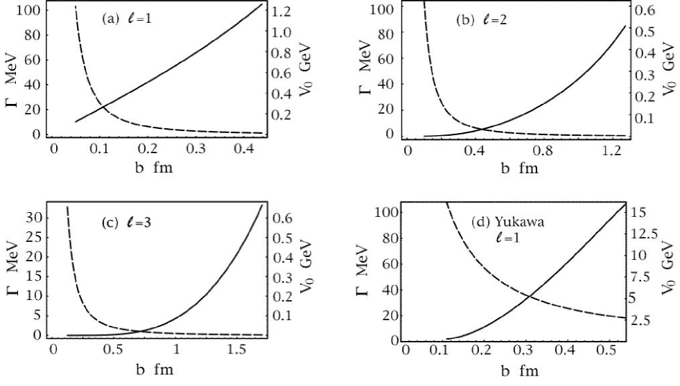
Figure 1: The width of the $\Theta$ in MeV as a function of the range of the attractive potential in Fermis with the mass of the $\Theta$ held fixed at 1540 MeV, for a square well, with (a) $\ell=1$; (b) $\ell=2$; and (c) $\ell=3$; and for a Yukawa potential and $\ell=1$, (d). Also shown is the depth of the potential (dashed).

3. Feshbach Resonances in a Two Channel Model

Having failed to find a narrow $\Theta$ in a low partial wave in $KN$ potential scattering, we explore the possibility of adding the resonance by hand as a bound state in the $KN$ continuum which can decay to $KN$. We review the formulation and solution of this simple scattering problem since it is not so widely known.

In addition to the open $KN$ channel (of definite isospin) we introduce a second channel which only has discrete eigenstates in the energy range of interest. The two channels are coupled by an off-diagonal potential, $V_{12}(\vec{x})$, which without loss of generality we take to be real. We do not need to know the potential in channel-2. The potential in channel-1, $V_{11}(\vec{x})$, is also unimportant. Since it does not generate the resonance, it merely introduces a smooth background phase in the neighborhood of the narrow (by assumption) resonance generated by the bound state in channel-2. Therefore we set $V_{11}=0$. The Hamiltonian for this system is given by

$$\mathcal{H}=\begin{pmatrix}-\nabla^{2}&V_{12}(\vec{x})\\ V_{12}(\vec{x})&H_{22}\end{pmatrix}$$ (3)

As explained, we assume that $H_{22}$ has a bound state solution given by

$$H_{22}\phi={k_{0}}^{2}\phi,$$ (4)

with ${k_{0}}=\sqrt{2\mu E_{0}}$= 270 MeV. We want to solve coupled set of Schrödinger equations $\mathcal{H}\Psi=k^{2}\Psi$ with $\Psi=\bigl{(}\begin{smallmatrix}\psi_{1}\\ \psi_{2}\end{smallmatrix}\bigr{)}$,

$$-\nabla^{2}\psi_{1}(\vec{x})+V_{12}(\vec{x})\psi_{2}(\vec{x}) = k^{2}\psi_{1}(\vec{x})$$

$$H_{22}\psi_{2}(\vec{x})+V_{12}(\vec{x})\psi_{1}(\vec{x}) = k^{2}\psi_{2}(\vec{x})$$ (5)

to obtain the scattering amplitude in channel-1. The particular solution for the second equation can be written in terms of the Green’s function in channel-2,

$$\psi_{2}(\vec{x})=-\int G_{22}(\vec{x},\vec{x}\ ^{\prime};k)V_{12}(\vec{x}\ ^{\prime})\psi_{1}(\vec{x}\ ^{\prime})d\vec{x}\ ^{\prime}$$ (6)

Note the absence of a solution, $\psi^{(0)}_{2}(\vec{x})$, to the homogeneous equation, $\left(H_{22}-k^{2}\right)\psi^{(0)}_{2}(\vec{x})=0$, which is excluded because there is no incoming wave in this confined/closed channel.

This problem is simplified dramatically because the resonance is narrow. Therefore we are only interested in values of $k$ close to $k_{0}$. In that region $G_{22}$ is dominated by the single pole associated with the state $\phi$,

$$G_{22}(\vec{x},\vec{x}\ ^{\prime};k)\approx-\frac{\phi(\vec{x})\phi(\vec{x}\ ^{\prime})}{{k_{0}}^{2}-k^{2}}\quad\mbox{for}\quad k\approx k_{0}$$ (7)

Note $\phi(x)$ can be taken to be real without loss of generality. Substituting eq. (7), together with eq. (6) into the first of eqs. (5) we obtain an integro-differential equation for $\psi_{1}$:

$$-\nabla^{2}\psi_{1}(\vec{x})-\int d\vec{x}^{\prime}\frac{\phi(\vec{x})\phi(\vec{x}\ ^{\prime})V_{12}(\vec{x})V_{12}(\vec{x}\ ^{\prime})}{{k_{0}}^{2}-k^{2}}\psi_{1}(\vec{x}\ ^{\prime})=k^{2}\psi_{1}(\vec{x}).$$ (8)

Although the potential in this effective Schrödinger equation is non-local, it is separable, and therefore amenable to an analytic treatment. The form of eq. (8) explains the physics: if $V_{12}$ is “small” and $k$ is not close to $k_{0}$, then there is no interaction and $\psi_{1}$ is a free continuum state — there is no scattering. However, no matter how small $V_{12}$ is, as long as it is not identically zero, there are values of $k$ close to $k_{0}$ for which the potential in eq. (8) is arbitrarily strong and attractive. Therefore there is always a resonance at $k\approx k_{0}$ and its width is controlled by the magnitude of $V_{12}$.

Conservation of angular momentum requires $V_{12}(\vec{x})$ and $H_{22}$ to be spherically symmetric. We assume that the bound state in channel-2 occurs in the $\ell^{\rm th}$ partial wave, in which case eq. (8) reduces to

$$-u_{\ell}^{\prime\prime}(r)+\frac{\ell(\ell+1)}{r^{2}}u_{\ell}(r)-\frac{V_{12}(r)v_{\ell}(r)}{{k_{0}}^{2}-k^{2}}\int dr^{\prime}V_{12}(r^{\prime})v_{\ell}(r^{\prime})u_{\ell}(r^{\prime})=k^{2}u_{\ell}(r)$$ (9)

where $\psi_{1}(\vec{x})=\frac{1}{r}u_{\ell}(r)Y_{\ell m}(\Omega)$ and $\phi(\vec{x})=\frac{1}{r}v_{\ell}(r)Y_{\ell m}(\Omega)$. We require $u_{\ell}(r)/r$ to be regular at the origin. For $V_{12}\equiv 0$ the solution of the above equation is given by ${\mathcal{U}}_{\ell}\propto krj_{\ell}(kr)$; for non-vanishing $V_{12}$ the solution can be written,

$$u_{\ell}^{(+)}(r)={\mathcal{U}}_{\ell}(r)+\int_{0}^{\infty}dr^{\prime}G_{\ell}^{(+)}(r,r^{\prime};k)\frac{V_{12}(r^{\prime})v_{\ell}(r^{\prime})}{{k_{0}}^{2}-k^{2}}\int_{0}^{\infty}dr^{\prime\prime}V_{12}(r^{\prime\prime})v_{\ell}(r^{\prime\prime})u_{\ell}^{(+)}(r^{\prime\prime}),$$ (10)

where we choose the Greens function $G_{\ell}^{(+)}$ to obey outgoing wave boundary conditions corresponding to scattering,

$$\begin{split}G_{\ell}^{(+)}(r,r^{\prime};k)&=\imath krr^{\prime}j_{\ell}(kr_{<})h_{\ell}^{(1)}(kr_{>})\\ &=\frac{rr^{\prime}}{\pi}\int_{-\infty}^{\infty}dq~{}q^{2}\frac{h_{\ell}^{(1)}(qr)j_{\ell}(qr^{\prime})}{q^{2}-k^{2}-\imath\epsilon}.\end{split}$$ (11)

We solve eq. (10) by multiplying by $V_{12}(r)v_{\ell}(r)$ and integrating over $r$. Using the Cauchy integral representation for the Green’s function, we obtain,

$$\eta_{\ell}(k)=\frac{\xi_{\ell}(k)}{1-\frac{X_{\ell}(k^{2})}{{k_{0}}^{2}-k^{2}}}$$ (12)

where

$$\eta_{\ell}(k) = \int_{0}^{\infty}dru_{\ell}^{(+)}(r)V_{12}(r)v_{\ell}(r)$$

$$\xi_{\ell}(k) = \int_{0}^{\infty}drrj_{\ell}(kr)V_{12}(r)v_{\ell}(r)$$ (13)

and

$$X_{\ell}(k^{2})=\frac{2}{\pi}\int\limits_{0}^{\infty}dq\frac{q^{2}}{q^{2}-k^{2}-\imath\epsilon}|\xi_{\ell}(q)|^{2}.$$ (14)

To extract the scattering amplitude we take the limit $r\to\infty$ in eq. (10) and compare with the expected form

$$\lim\limits_{r\rightarrow\infty}u_{\ell}^{(+)}(r)=e^{\imath\delta_{\ell}(k)}\sin(kr-\frac{\ell\pi}{2}+\delta_{\ell}(k)),$$ (15)

from which we obtain the following partial wave scattering amplitude

$$kf_{\ell}(k)\equiv e^{\imath\delta_{\ell}(k)}\sin\delta_{\ell}(k)=\frac{{k}|\xi_{\ell}(k)|^{2}}{{k_{0}}^{2}-k^{2}-X_{\ell}(k)}.$$ (16)

This constitutes a complete solution to the problem because $\xi_{\ell}(k)$ and $X_{\ell}(k)$ depend only on the known functions $V_{12}(r),v_{\ell}(r)$ and the free wavefunction $rj_{\ell}(kr)$.

To leading order in the (small) channel coupling the resonance occurs at $k_{0}$ and has width,

$$\Gamma_{\ell}(k_{0})=\frac{k_{0}}{\mu}|\xi_{\ell}(k_{0})|^{2},$$ (17)

$\Gamma_{\ell}$ depends strongly on $k_{0}$ through the dependence of $\xi_{\ell}(k)$ on $j_{\ell}(kr)$.

The width $\Gamma_{\ell}$ depends only on the product of $V_{12}(r)$ and $v_{\ell}(r)$. For simplicity we once again take a square well, $V_{12}(r)=-2\mu\Omega\theta(b-r)$, and we take $v_{\ell}(r)/r$ to be the nodeless $\ell$-wave bound state solution for the infinite square well of range $b$ and depth adjusted such that the energy of the state is $k_{0}^{2}/2\mu$. The results do not depend significantly on these choices because we normalize the parameters to the known width of the $\Lambda(1520)$. In this simple case the width of the resonance in $\ell^{\rm th}$ partial wave is given by

$$\Gamma_{\ell}(k_{0})=8\chi_{\ell}^{2}\mu\Omega^{2}k_{0}b^{3}\frac{j_{\ell}^{2}(k_{0}b)}{\bigl{[}\chi_{\ell}^{2}-k_{0}^{2}b^{2}\bigr{]}^{2}},$$ (18)

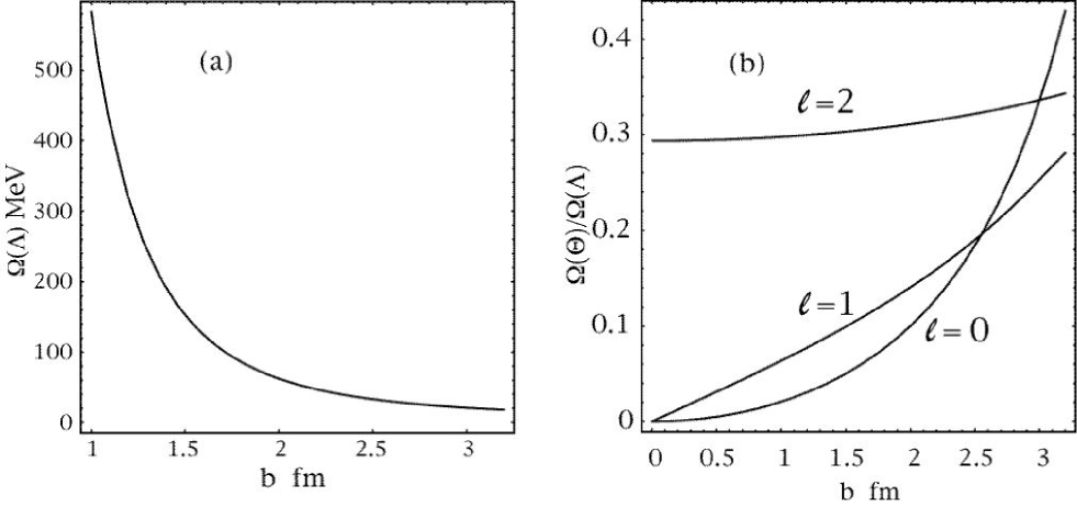
Figure 2: (a) The strength of the channel coupling potential responsible for the width of the $\Lambda(1520)$ in the Feshbach-Fano formalism (see eq. (18)). (b) Ratio of the channel coupling potential strengths for the $\Theta$ and $\Lambda(1520)$ for various assignments of the orbital angular momentum in the $\Theta$ channel.

where $\chi_{\ell}$ is the first zero of $j_{\ell}(x)$.

This result allows us to relate the range, $b$, and the strength, $\Omega$, of the channel coupling to the width of the resonance as a function of $\ell$. Fortunately, as we have noted in the introduction, Nature has provided us with a conventional non-exotic $\overline{K}N$ resonance, the $\Lambda(1520)$ at nearly the same mass as the $\Theta^{+}(1540)$. The $\Lambda(1520)$ is not a controversial resonance. It is usually described as a $p$-wave $uds$ state, and for the purposes of this analysis we can represent it in $\overline{K}N$ scattering as a Feshbach resonance. The analysis we have just completed therefore applies without alteration to the $\Lambda(1520)$. It appears in the $d$-wave and has a partial width into $\overline{K}N$ of 7 MeV, so we have enough information to use eq. (18) to determine $\Omega(\Lambda)$ as a function of $b$. This is shown in Fig. 2(a). This, in turn, enables us to normalize the values of $\Omega$ needed to account for the width of the $\Theta^{+}(1540)$. It is a simple matter to determine the value of $\Omega(\Theta)$ for some fiducial value of $\Gamma(\Theta)$ and compare it with $\Omega(\Lambda)$ as a function of $b$ and $\ell$. Our results are shown in Fig. 2(b). There we plot the ratio $\Omega_{\ell}(\Theta)/\Omega(\Lambda)$ as a function of $b$ for $\ell=0,1$ and 2. In Fig. 2(b) we have assumed $\Gamma(\Theta)=1$ MeV. When the width of the $\Theta$ is measured one can obtain the actual value of $\Omega_{\ell}(\Theta)/\Omega(\Lambda)$ by multiplying the result(s) shown in the figure by $\sqrt{\Gamma(\Theta)}$ in MeV^1/2. The trends in Fig. 2(b) are easy to understand. As $b$ decreases the channel coupling occurs at distances where $rj_{\ell}(kb)$ decreases like $kb^{\ell+1}$. To account for the width of the ($d$-wave) $\Lambda(1520)$, $\Omega(\Lambda)$ must increase rapidly as $b\to 0$. If the $\Theta$ also appears in the $d$-wave its width scales the same way as the $\Lambda(1520)$’s and the ratio is only weakly dependent on $b$. It would be exactly constant if the masses of the $\Theta$ and the $\Lambda(1520)$ were equal. If the $\Theta$ appears in a lower partial wave its width decreases more slowly as $b\to 0$, so the value of $\Omega(\Theta)$ must decrease relative to $\Omega(\Lambda)$ in order to keep $\Gamma(\Theta)$ fixed at 1 MeV. Thus as $b\to 0$ the channel coupling of the $\Theta$ becomes progressively more unnatural. At $b=1$ fm. the ratio $\Omega(\Theta)/\Omega(\Lambda)$ must be 0.02 for $\ell=0$, 0.06 for $\ell=1$, 0.3 for $\ell=2$. It is in this sense that the a width of 1 MeV for the $\Theta$ is extraordinary compared to the width of the conventional $\Lambda(1520)$ resonance. A theorist attempting to understand the width of the $\Theta$ implemented as a confined state appearing in the $KN$ $s$- or $p$-wave, must explain why its coupling to the open channel is suppressed compared to the coupling of a state (the $\Lambda(1520)$) with a natural suppression mechanism. The small width of the $\Theta$ presents a challenge to model builders even when it is introduced by hand as a Feshbach resonance.

References

- (1) For a recent review of the experimental situation see, G. Trilling in S. Eidelman et al. [Particle Data Group Collaboration], Phys. Lett. B 592, 1 (2004).
- (2) For a summary see T. Nakano and K. Hicks, Mod. Phys. Lett. A 19, 645 (2004).
- (3) R. N. Cahn and G. H. Trilling, Phys. Rev. D 69, 011501 (2004) [arXiv:hep-ph/0311245].
- (4) S. Nussinov, arXiv:hep-ph/0307357.
- (5) R. A. Arndt, I. I. Strakovsky and R. L. Workman, Phys. Rev. C 68, 042201 (2003) [Erratum-ibid. C 69, 019901 (2004)] [arXiv:nucl-th/0308012].
- (6) A. Sibirtsev, J. Haidenbauer, S. Krewald and U. G. Meissner, Phys. Lett. B 599, 230 (2004) [arXiv:hep-ph/0405099].
- (7) See Ref. trilling for further references and discussion.
- (8) U. Fano, Nuovo Cim. 12, 154 (1935), Phys. Rev. 124 1866 (1961).
- (9) H. Feshbach, Ann. Phys. 5, 357 (1958).
- (10) This case was mentioned in Ref. jw1
- (11) R. L. Jaffe and F. Wilczek, Phys. Rev. Lett. 91, 232003 (2003) [arXiv:hep-ph/0307341].
- (12) D. Diakonov, V. Petrov and M. V. Polyakov, Z. Phys. A 359, 305 (1997) [arXiv:hep-ph/9703373].
- (13) For a critical discussion of Ref. dpp , see R. L. Jaffe, Eur. Phys. J. C 35, 221 (2004) [arXiv:hep-ph/0401187]; D. Diakonov, V. Petrov and M. Polyakov, arXiv:hep-ph/0404212; R. L. Jaffe, arXiv:hep-ph/0405268.
- (14) M. P. Mattis and M. Karliner, Phys. Rev. D 31, 2833 (1985); Phys. Rev. D 34, 1991 (1986); N. Itzhaki, I. R. Klebanov, P. Ouyang and L. Rastelli, Nucl. Phys. B 684, 264 (2004) [arXiv:hep-ph/0309305].
- (15) M. Karliner and H. J. Lipkin, arXiv:hep-ph/0307243, and Phys. Lett. B 575, 249 (2003) [arXiv:hep-ph/0402260].
- (16) J. J. Sakurai, Modern Quantum Mechanics (Addison-Wesley, 1994).