Observables sensitive to absolute neutrino masses:
Constraints and correlations from world neutrino data

Abstract

In the context of three-flavor neutrino mixing, we present a thorough study of the phenomenological constraints applicable to three observables sensitive to absolute neutrino masses: The effective neutrino mass in Tritium beta decay $(m_{\beta})$; the effective Majorana neutrino mass in neutrinoless double beta decay $(m_{\beta\beta})$; and the sum of neutrino masses in cosmology $(\Sigma)$. We discuss the correlations among these variables which arise from the combination of all the available neutrino oscillation data, in both normal and inverse neutrino mass hierarchy. We set upper limits on $m_{\beta}$ by combining updated results from the Mainz and Troitsk experiments. We also consider the latest results on $m_{\beta\beta}$ from the Heidelberg-Moscow experiment, both with and without the lower bound claimed by such experiment. We derive upper limits on $\Sigma$ from an updated combination of data from the Wilkinson Microwave Anisotropy Probe (WMAP) satellite and the 2 degrees Fields (2dF) Galaxy Redshifts Survey, with and without Lyman-$\alpha$ forest data from the Sloan Digital Sky Survey (SDSS), in models with a non-zero running of the spectral index of primordial inflationary perturbations. The results are discussed in terms of two-dimensional projections of the globally allowed region in the $(m_{\beta},m_{\beta\beta},\Sigma)$ parameter space, which neatly show the relative impact of each data set. In particular, the (in)compatibility between $\Sigma$ and $m_{\beta\beta}$ constraints is highlighted for various combinations of data. We also briefly discuss how future neutrino data (both oscillatory and non-oscillatory) can further probe the currently allowed regions.

I introduction

Atmospheric Atmo ; SKLE ; MACR ; Soud , solar Home ; SAGE ; GALL ; Catt ; SKso ; SNOs , reactor KamL ; Grat ; KL04 and accelerator K2K1 ; K2K2 neutrino experiments have convincingly established that neutrinos are massive and mixed Pont ; Maki . World neutrino data (with a single controversial exception LSND ) are consistent with a three-flavor mixing framework Conc ; Barg ; Keow ; Ours ; Malt ; Srub , parameterized in terms of three neutrino masses $(m_{1},m_{2},m_{3})$ and of three mixing angles $(\theta_{12},\theta_{23},\theta_{13})$ PDG4 , plus a possible CP violating phase $\delta$ Kays .

Neutrino oscillation experiments are sensitive to two independent squared mass difference, $\delta m^{2}$ and $\Delta m^{2}$ (with $\delta m^{2}\ll\Delta m^{2}$), hereafter defined as Delt

$$(m^{2}_{1},m^{2}_{2},m^{2}_{3})=\mu^{2}+\left(-\frac{\delta m^{2}}{2},+\frac{\delta m^{2}}{2},\pm\Delta m^{2}\right),$$ (1)

where $\mu$ fixes the absolute neutrino mass scale, while the cases $+\Delta m^{2}$ and $-\Delta m^{2}$ identify the so-called normal and inverted neutrino mass hierarchies, respectively. Neutrino oscillation data indicate that $\delta m^{2}\simeq 8\times 10^{-5}$ eV² KL04 and $\Delta m^{2}\simeq 2.4\times 10^{-3}$ eV² SKLE ; K2K2 . They also indicate that $\sin^{2}\theta_{12}\simeq 0.3$ KL04 , $\sin^{2}\theta_{23}\simeq 0.5$ SKLE ; K2K2 , and $\sin^{2}\theta_{13}\lesssim\mathrm{few}\%$ CHOO . However, they are currently unable to determine the mass hierarchy ($\pm\Delta m^{2}$) and the phase $\delta$ Kays , and are insensitive to the absolute mass parameter $\mu$ in Eq. (1).

The absolute neutrino mass scale can be probed by non-oscillatory neutrino experiments. The most sensitive laboratory experiments to date have been focussed on tritium beta decay Holz ; Wein ; Mass and on neutrinoless double beta decay Doub ; Vo02 ; Elli . Beta decay experiments probe the so-called effective electron neutrino mass $m_{\beta}$ Mbet ,

$$m_{\beta}=\left[c^{2}_{13}c^{2}_{12}m^{2}_{1}+c^{2}_{13}s^{2}_{12}m^{2}_{2}+s^{2}_{13}m^{2}_{3}\right]^{\frac{1}{2}}\ ,$$ (2)

where $c^{2}_{ij}=\cos^{2}\theta_{ij}$ and $s^{2}_{ij}=\sin^{2}\theta_{ij}$. Current experiments (Mainz Main and Troitsk Troi ) provide upper limits in the range $m_{\beta}\lesssim\mathrm{few}$ eV PDG4 ; Eite .

Neutrinoless double beta decay ($0\nu 2\beta$) experiments are instead sensitive to the so-called effective Majorana mass $m_{\beta\beta}$ (if neutrinos are Majorana fermions) Wo81 ; BiPe ,

$$m_{\beta\beta}=\left|c^{2}_{13}c^{2}_{12}m_{1}+c^{2}_{13}s^{2}_{12}m_{2}e^{i\phi_{2}}+s^{2}_{13}m_{3}e^{i\phi_{3}}\right|\ ,$$ (3)

where $\phi_{2}$ and $\phi_{3}$ parameterize relative (and unknown) Majorana neutrino phases ScVa . All $0\nu 2\beta$ experiments place only upper bounds on $m_{\beta\beta}$ (the most sensitive being in the eV range Elli ), with the exception of the Heidelberg-Moscow experiment Kl01 , which claims a positive (but highly debated Elli ) $0\nu 2\beta$ signal, corresponding to $m_{\beta\beta}$ in the sub-eV range at best fit Kl03 ; Kl04 .

Recently, astrophysical and cosmological observations have started to provide indirect upper limits on absolute neutrino masses (see, e.g., the reviews Barg ; Mass ; Dolg ), competitive with those from laboratory experiments. In particular, the combined analysis of high-precision data from Cosmic Microwave Background (CMB) anisotropies and Large Scale Structures (LSS) has already reached a sensitivity of $O(\mathrm{eV})$ (see, e.g., Be03 ; Tg04 ; Laha ) for the sum of the neutrino masses $\Sigma$,

$$\Sigma=m_{1}+m_{2}+m_{3}\ .$$ (4)

We recall that the total neutrino energy density in our Universe, $\Omega_{\nu}h^{2}$ (where $h$ is the Hubble constant normalized to $H_{0}=100$ km s^-1 Mpc^-1) is related to $\Sigma$ by the well-known relation $\Omega_{\nu}h^{2}=\Sigma/(93.2\mathrm{\ eV})$ PDG4 , and plays an essential role in theories of structure formation. It can thus leave key signatures in LSS data (see, eg., Hu98 ) and, to a lesser extent, in CMB data (see, e.g., Ma95 ). Very recently, it has also been shown that accurate Lyman-$\alpha$ (Ly$\alpha$) forest data Mc04 , taken at face value, can improve the current CMB+LSS constraints on $\Sigma$ by a factor of $\sim 3$, with important consequences on absolute neutrino mass scenarios Se04 . Given the potentially large systematics of Ly$\alpha$ data Mc04 , we will conservatively perform and compare global cosmological fits both with and without Ly$\alpha$ constraints.

There is a vast literature about the theoretical and phenomenological links and correlations connecting [via Eqs. (1)–(4)] the $3\nu$ mass-mixing oscillation parameters $(\delta m^{2},\Delta m^{2},\theta_{ij})$ with the observables sensitive to absolute neutrino masses $(m_{\beta},m_{\beta\beta},\Sigma)$; see, e.g., the extensive bibliography in the reviews Barg ; Keow ; Mass ; Elli . These interesting correlations have often been studied and plotted in terms of an auxiliary variable, such as the lightest neutrino mass $m_{\mathrm{lightest}}$; in particular, many relevant papers have focussed on constraints in the $(m_{\beta\beta},m_{\mathrm{lightest}})$ plane (see, e.g., Ligh ; Simk ). However, since $m_{\mathrm{lightest}}$ is not directly measured, it can actually be removed from data analyses, by charting the results just in terms of the three measurable quantities $(m_{\beta},m_{\beta\beta},\Sigma)$.

In this work we undertake a global phenomenological analysis of the constraints applicable to the observables $(m_{\beta},m_{\beta\beta},\Sigma)$, by using up-to-date experimental data and state-of-the-art calculations for all the relevant laboratory and astrophysical quantities. To our knowledge, this is the first attempt to fitting world neutrino data, both oscillatory and non-oscillatory, in the “standard” astroparticle physics scenario emerged in the last few years (i.e., standard $3\nu$ mixing plus standard cosmology). The results are shown and discussed in terms of allowed regions in each of the three 2-dimensional projections of the parameter space $(m_{\beta},m_{\beta\beta},\Sigma)$, for both normal and inverted hierarchy. Such projections neatly show the interplay among different observables, as well as the impact of each data set. In particular, a tension is seen to emerge between current constraints on $\Sigma$ and $m_{\beta\beta}$. Our synthesis of world neutrino data appears also useful for estimating the sensitivity required by future experiments in order to solve, e.g., the mass hierarchy ambiguity, or to probe Majorana phases.

The structure of the paper is as follows. In Secs. II, III, IV, and V we describe our treatment of the relevant input from oscillation, beta-decay, $0\nu 2\beta$, and cosmological data, respectively. In Sec. VI we discuss the bounds on $(m_{\beta},m_{\beta\beta},\Sigma)$ coming from neutrino oscillation data only, with emphasis on the correlations among couples of observables. In Sec. VII we combine the previous results with the upper bounds on $(m_{\beta},m_{\beta\beta},\Sigma)$ coming from laboratory experiments and cosmological CMB+LSS data (without Ly$\alpha$ forest data). In Sec. VIII we implement a possible lower bound on $m_{\beta\beta}$ based on the claim in Kl03 ; Kl04 , and describe its effect on the global fit. Finally, in Sec. IX we discuss the impact of recent Ly$\alpha$ data Mc04 ; Se04 . We draw our conclusions in Sec. X.

II Input from $\nu$ oscillation data

In this work, we perform an updated global analysis of oscillation neutrino data including: Atmospheric Super-Kamiokande (SK) data SKLE ; solar data from the Chlorine (Cl) Home , Gallium (Ga) SAGE ; GALL ; Catt , SK SKso , and Sudbury Neutrino Observatory (SNO) SNOs experiments; reactor data from the KamLAND KamL ; KL04 and CHOOZ CHOO experiments; and KEK-to-Kamioka (K2K) accelerator data K2K1 ; K2K2 . We refer the reader to previous works Prev for details of the analysis. We include the latest experimental data presented at the Neutrino 2004 Conference Catt ; Grat ; K2K2 . In particular, we make a $3\nu$ analysis of the available solar and KamLAND data, which are sensitive to the mass-mixing parameters $(\delta m^{2},\sin^{2}\theta_{12},\sin^{2}\theta_{13})$. We derive the likelihood of the $\Delta m^{2}$ parameter from a graphical reduction and combination of the corresponding likelihoods determined by the SK atmospheric SKLE and K2K accelerator K2K2 experiments in the $2\nu$ limit, marginalized with respect to $\theta_{23}$. The probability distribution of $\Delta m^{2}$ is crucial to obtain upper bounds on $\theta_{13}$ from the CHOOZ reactor experiment Th13 . The results of our analysis of neutrino oscillation data are embedded in a $\chi^{2}$ fit function,

$$\chi^{2}_{\mathrm{osc}}(\delta m^{2},\Delta m^{2},\sin^{2}\theta_{12},\sin^{2}\theta_{13})=$$ (5)

$$\chi^{2}_{\mathrm{solar+KamL}}(\delta m^{2},\sin^{2}\theta_{12},\sin^{2}\theta_{13})+$$

$$\chi^{2}_{\mathrm{SK+K2K}}(\Delta m^{2})+\chi^{2}_{\mathrm{CHOOZ}}(\Delta m^{2},\sin^{2}\theta_{13})\ ,$$

which provides the likelihood for the four oscillation parameters $(\delta m^{2},\Delta m^{2},\sin^{2}\theta_{12},\sin^{2}\theta_{13})$ needed for the calculation of the $(m_{\beta},m_{\beta\beta},\Sigma)$ observables.

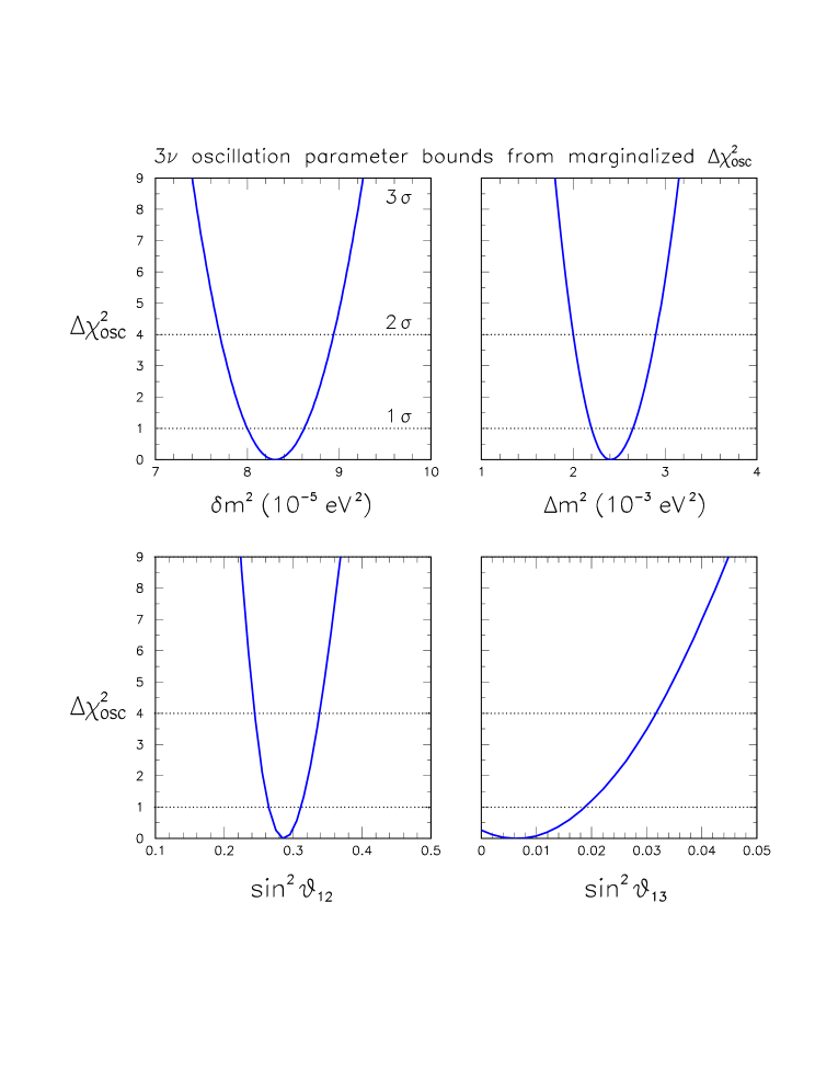
Figure 1: Bounds on the $3\nu$ mass-mixing neutrino parameters $(\delta m^{2},\Delta m^{2},\sin^{2}\theta_{12},\sin^{2}\theta_{13})$ from our analysis of current neutrino oscillation data. The solid curves represent projections of the $\Delta\chi^{2}_{\mathrm{osc}}$ fit function. The intercepts of the curves with the horizontal dotted lines at $\Delta\chi^{2}=n^{2}$ define the $n$-$\sigma$ limits on each parameter. There is no statistically significant lower limit for $\sin^{2}\theta_{13}$.

Figure 1 shows the function $\Delta\chi^{2}_{\mathrm{osc}}=\chi^{2}_{\mathrm{osc}}-\min\chi^{2}_{\mathrm{osc}}$ from the global $\nu$ oscillation data fit, marginalized with respect to each of its four arguments. The condition $\Delta\chi_{\mathrm{osc}}^{2}=n^{2}$ provides $n$-$\sigma$ bounds on each mass-mixing parameter. At best fit we find

$$\sqrt{\delta m^{2}} \simeq 9.1\times 10^{-3}\mathrm{\ eV}\ ,$$ (6)

$$\sqrt{\Delta m^{2}} \simeq 4.9\times 10^{-2}\mathrm{\ eV}\ ,$$ (7)

and

$$\sin^{2}\theta_{12} \simeq 0.29\ ,$$ (8)

$$\sin^{2}\theta_{13} \simeq 0.007\ .$$ (9)

Notice, however, that the slight preference for nonzero $\sin^{2}\theta_{13}$ in Fig. 1 is not statistically significant.

III Input from Tritium $\beta$-decay data

Updated determinations of the effective electron neutrino mass squared $m^{2}_{\beta}$ have been recently presented Eite for the Mainz Main and Troitsk Troi tritium $\beta$-decay experiments. The experimental values are consistent with zero within errors:

$$m^{2}_{\beta} = -1.2\pm 3.0\mathrm{\ eV}^{2}\ (\mathrm{Mainz})\ ,$$ (10)

$$m^{2}_{\beta} = -2.3\pm 3.2\mathrm{\ eV}^{2}\ (\mathrm{Troitsk})\ ,$$ (11)

where errors are at $1\sigma$ level, and systematic and statistical components have been added in quadrature. The $\chi^{2}_{\beta}$ function associated to the above $\beta$-decay data can be simply defined as:

$$\chi^{2}_{\beta,X}(m_{\beta})=\left(\frac{m^{2}_{\beta}-m^{2}_{\beta,X}}{\sigma_{\beta,X}}\right)^{2}\ ,$$ (12)

where $m^{2}_{\beta,X}$ and $\sigma_{\beta,X}$ are the central values and errors on the right hand side of Eqs. (10) and (11), for $X=\mathrm{Mainz}$ and $X=\mathrm{Troitsk}$, respectively. By restricting the domain to the physical region ($m^{2}_{\beta}\geq 0$), the $\Delta\chi^{2}$ function relevant for our analysis becomes

$$\Delta\chi^{2}_{\beta,X}(m_{\beta})=\chi^{2}_{\beta,X}(m_{\beta})-\chi^{2}_{\beta,X}(0)\ ,$$ (13)

providing the following upper bounds at 95% C.L. ($\Delta\chi^{2}\simeq 4$),

$$m_{\beta} < 2.2\mathrm{\ eV}\ (\mathrm{Mainz})\ ,$$ (14)

$$m_{\beta} < 2.1\mathrm{\ eV}\ (\mathrm{Troitsk})\ ,$$ (15)

in agreement with the upper bounds quoted by the experimental collaborations Eite .

It is matter of debate whether the two experiments have common systematics, e.g., responsible for the negative central value of $m^{2}_{\beta}$ (see Brad for a recent discussion). In the absence of a clear indication in this sense, we assume that the two experimental results are independent, and simply combine them through

$$\Delta\chi^{2}_{\beta}(m_{\beta})=\Delta\chi^{2}_{\beta,\mathrm{Mainz}}(m_{\beta})+\Delta\chi^{2}_{\beta,\mathrm{Troitsk}}(m_{\beta})\ .$$ (16)

From the above definition, we get a combined upper limit at 95% C.L.,

$$m_{\beta}<1.8~{}\mathrm{eV}\ (\mathrm{Mainz}+\mathrm{Troitsk})\ ,$$ (17)

which is less conservative than the $3$ eV upper limit recommended in PDG4 . However, as we will see, upper limits on $m_{\beta}$ in the 2–3 eV range are, in any case, too weak to contribute significantly to the current global fit in the $(m_{\beta},m_{\beta\beta},\Sigma)$ parameter space, so that “conservativeness” is not (yet) an issue in this context.

IV Input from Germanium $0\nu 2\beta$ decay data

Neutrinoless double beta decay processes of the kind $(Z,A)\to(Z+2,A)+2e^{-}$ have been searched in many experiments with different isotopes, yielding negative results (see Vo02 ; Elli for reviews). Recently, members of the Heidelberg-Moscow experiment HMex have claimed the detection of a $0\nu 2\beta$ signal from the ⁷⁶Ge isotope Kl01 ; Kl03 ; Kl04 . The claimed signal would correspond to a decay half-life $T$ in years (y) within the following $3\sigma$ interval Kl03 ; Kl04 :

$$\log_{10}(T/\mathrm{y})=25.08^{+0.54}_{-0.24}\ (3\sigma)\ .$$ (18)

If the $0\nu 2\beta$ signal is entirely due to light Majorana neutrino masses, the half-life $T$ is related to the $m_{\beta\beta}$ parameter in Eq. (3) by the relation

$$m^{2}_{\beta\beta}=\frac{m^{2}_{e}}{C_{mm}T}\ ,$$ (19)

where $m_{e}$ is the electron mass and $C_{mm}$ is the nuclear matrix element for the considered isotope Elli .

Unfortunately, theoretical uncertainties on $C_{mm}$ are rather large (see e.g. Elli ), and their—somewhat arbitrary—estimate is matter of debate (see Simk ; Civi ; Bahc and refs. therein). Our approach to estimate a central value and an error for matrix element $C_{mm}$ relevant to ⁷⁶Ge experiments is the following. We take from the list of “acceptable” $C_{mm}$ calculations (i.e., calculations with no subsequently recognized errors or biases) discussed in Elli the “extremal” estimates: $\log_{10}(C_{mm}^{\mathrm{min}}/\mathrm{y}^{-1})=-13.85$ Mini and $\log_{10}(C_{mm}^{\mathrm{max}}/\mathrm{y}^{-1})=-12.88$ Maxi . Then we assume that their half-sum and their difference define, respectively, the central value and the $3\sigma$ uncertainty (in log scale), namely: $\log_{10}(C_{mm}^{0}/\mathrm{y}^{-1})=-13.36$ and $3\sigma\equiv 13.85-12.88=0.97$. We thus take

$$\log_{10}(C_{mm}/\mathrm{y}^{-1})=-13.36\pm 0.97\ (3\sigma)$$ (20)

which embeds a rather conservative error estimate—the $3\sigma$ uncertainty being almost equal to an order of magnitude variation in $C_{mm}$, as also evaluated in Bahc . The above central value for $C_{mm}$ is close to recent detailed theoretical calculations Rodi .

From the previous equations, under the assumption of a positive $0\nu 2\beta$ signal in Ref. Kl03 ; Kl04 , we derive that

$$\log_{10}(m_{\beta\beta}/\mathrm{eV}) = \log_{10}(m_{e}/\mathrm{eV})-\frac{1}{2}\log_{10}(C_{mm}/\mathrm{y}^{-1})-\frac{1}{2}\log_{10}(T/\mathrm{y})$$ (21)

$$= 5.71+\frac{1}{2}(13.36\pm 0.97)-\frac{1}{2}\left(25.08^{+0.54}_{-0.24}\right)\$$ (22)

$$= -0.23\pm 0.53\ (3\sigma)\ ,$$ (23)

where, in the last line, we have symmetrized the asymmetric range $25.08^{+0.54}_{-0.24}$ as $25.23\pm 0.39$ (according to the recipe suggested in Dago ) before adding the errors in quadrature (see Dago for the statistical rationale of this procedure). Equation (23) allows us to define the $\Delta\chi^{2}_{\beta\beta}(m_{\beta\beta})$ function associated to the claim in Ref. Kl03 ; Kl04 , and provides the $3\sigma$ range $0.17<m_{\beta\beta}<2.0$ (in eV).

The claim in Kl03 ; Kl04 has been subject to strong criticism, especially after the first publication Kl01 (see Elli and refs. therein). Therefore, we will also consider the possibility that $T=\infty$ is allowed (i.e., that there is no $0\nu 2\beta$ signal), in which case the experimental lower bound on $m_{\beta\beta}$ disappears. Since one cannot really reprocess the data of Kl03 ; Kl04 under the assumption of no signal, nor combine such data with the negative results of other experiments with comparable sensitivity to $m_{\beta\beta}$ Elli , the definition of a $\Delta\chi^{2}_{\beta\beta}(m_{\beta\beta})$ function in the absence of a $0\nu 2\beta$ signal is somewhat ambiguous and, in part, arbitrary. Our approach simply consists in stretching the lower error in Eq. (23) to infinity, so that the lower bound on $m_{\beta\beta}$ disappears, while the upper bound remains in the $O(\mathrm{eV})$ ballpark indicated by the most sensitive experiments to date Elli . It is worth noticing that none of the main results of our work depends on the precise definition of the upper bound on $m_{\beta\beta}$.

In conclusion, we adopt the following two possible $0\nu 2\beta$ inputs (and associated $\Delta\chi^{2}_{\beta\beta}$ functions) for our global analysis:

$$\log_{10}(m_{\beta\beta}/\mathrm{eV}) = -0.23\pm 0.18\ (0\nu 2\beta\mathrm{\ signal\ assumed})\ ,$$ (24)

$$\log_{10}(m_{\beta\beta}/\mathrm{eV}) = -0.23^{+0.18}_{-\infty}\ (0\nu 2\beta\mathrm{\ signal\ not\ assumed})\ ,$$ (25)

where errors are at $1\sigma$ level. Concerning the unknown Majorana phases $\phi_{2}$ and $\phi_{3}$ in Eq. (3), we simply assume that they are independent and uniformly distributed in the range $[0,\pi]$.

V Input from cosmological data

The neutrino contribution to the overall energy density of the universe can play a relevant role in large scale structure formation and leave key signatures in several cosmological data sets. More specifically, neutrinos suppress the growth of fluctuations on scales below the horizon when they become non relativistic. A massive neutrinos of a fraction of eV would therefore produce a significant suppression in the clustering on small cosmological scales (namely, for comoving wavenumber $k\sim 0.05\ h\ \mathrm{Mpc}^{-1}$).

To constrain $\Sigma$ from cosmological data, we perform a likelihood analysis comparing the recent observations with a set of models with cosmological parameters sampled as follows: cold dark matter (cdm) density $\Omega_{\mathrm{cdm}}h^{2}\in[0.05,0.20]$ in steps of $0.01$; baryon density $\Omega_{b}h^{2}\in[0.015,0.030]$ (motivated by Big Bang Nucleosynthesis) in steps of $0.001$; a cosmological constant $\Omega_{\Lambda}\in[0.50,0.96]$ in steps of $0.02$; and neutrino density $\Omega_{\nu}h^{2}\in[0.001,0.020]$ in steps of $0.002$. We restrict our analysis to flat $\Lambda$-CDM models, $\Omega_{\mathrm{tot}}=1$, and we add a conservative external prior on the age of the universe, $t_{0}>10$ Gyrs. The use of a method based on a database of models instead of Markov Chains (see e.g. Be03 ) has the advantage of being more reliable in the definition of likelihood confidence contours at more than 3$\sigma$ level. No alternative model to a cosmological constant is considered: the dark energy is described by an unclustered fluid with constant equation of state ($w=-1$). Variations in the equation of state affect mainly curvature parameters (see, e.g., bean ) and therefore do not alter our results on $\Sigma$.

The value of the Hubble constant in our database is not an independent parameter, since it is determined through the flatness condition. We adopt the conservative top-hat bound $0.50<h<0.90$ and we also consider the $1\sigma$ constraint on the Hubble parameter, $h=0.71\pm 0.07$, obtained from Hubble Space Telescope (HST) measurements freedman . We allow for a reionization of the intergalactic medium by varying the CMB photon optical depth $\tau_{c}$ in the range $\tau_{c}\in[0.05,0.30]$ in steps of $0.02$.

We restrict the analysis to adiabatic inflationary models with a negligible contribution of gravity waves. We do not consider the possibility of isocurvature perturbations jxd or topological defects (see, e.g., dkm ). We let vary the spectral index $n$ of scalar primordial fluctuations in the range $n\in[0.85,1.3]$ and its running $dn/d\ln k\in[-0.40,0.2]$ assuming pivot scales at $k_{0}=0.05\mathrm{\ Mpc}^{-1}$ and $k_{0}=0.002\mathrm{\ Mpc}^{-1}$. We rescale the fluctuation amplitude by a prefactor $C_{110}$, in units of the value $C_{110}^{\mathrm{WMAP}}$ measured by the Wilkinsin Microwave Anisotropy Probe (WMAP) satellite. Finally, concerning the neutrino parameters, we fix the number of neutrino species to $N_{\nu}=3$, all with the same mass (the effect of mass differences compatible with neutrino oscillation being negligible in the current cosmological data pastor ). An higher number of neutrino species can weakly affect both CMB and LSS data (see, e.g., bowen ) but is highly constrained by standard big bang nucleosynthesis and is not considered in this work, where we focus on $3\nu$ mixing.

The cosmological data we considered comes from observation of CMB anisotropies and polarization, galaxy redshift surveys and luminosity distances of type Ia supernovae. For the CMB data we use the recent temperature and cross polarization results from the WMAP satellite Be03 using the method explained in map5 and the publicly available code on the LAMBDA web site LAMBDA . Given a theoretical temperature anisotropy and polarization angular power spectrum in our database, we can therefore associate a $\chi^{2}_{\mathrm{WMAP}}$ to the corresponding theoretical model.

We further include the latest results from the BOOMERanG-98 ruhl , Degree Angular Scale Interferometer (DASI) halverson , MAXIMA-1 lee , Cosmic Background Imager (CBI) pearson , and Very Small Array Extended (VSAE) clive experiments by using the publicly available correlation matrices, window functions and beam and absolute calibration errors. The CMB data analysis methods for the non-WMAP data have been already extensively described in various papers (see, e.g., mesilk ) and will not be reported here.

In addition to the CMB data we also consider the real-space power spectrum of galaxies from either the 2 degrees Fields (2dF) Galaxy Redshifts Survey or the Sloan Digital Sky Survey (SDSS), using the data and window functions of the analysis of thx and Tg04 . We restrict the analysis to a range of scales over which the fluctuations are assumed to be in the linear regime ($k<0.2h^{-1}\mathrm{\ Mpc}$). When combining with the CMB data, we marginalize over a bias $b$ for each data set considered as an additional free parameter.

We also include information from the Ly$\alpha$ Forest in the SDSS, using the results of the analysis of Se04 and Mc04 , which probe the amplitude of linear fluctuations at very small scales. For this data set, small-scale power spectra are computed at high redshifts and compared with the values presented in Mc04 . As in Se04 , we do not consider running.

We finally incorporate constraints obtained from the SN-Ia luminosity measurements of riess using the so-called GOLD data set. Luminosity distances at SN-Ia redshifts are computed for each model in our database and compared with the observed apparent bolometric SN-Ia luminosities.

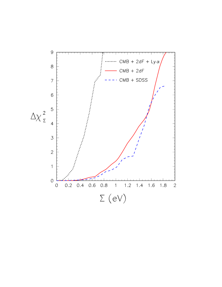
Figure 2: Upper bounds on the sum of neutrino masses $\Sigma$ from our $3\nu$ analysis of cosmological data, given in terms of the $\Delta\chi^{2}_{\Sigma}$ function. The solid and dashed curves refer to the combination of CMB and LSS data (CMB+2dF and CMB+SDSS, respectively). The two CMB+LSS fits provide comparable results and, for definiteness, the CMB+2df one is adopted. In addition, we consider also the case where the recent Ly$\alpha$ data from the SDSS are included, providing significantly stronger constraints on $\Sigma$ (dotted curve). See the text for details.

In Fig. 2 we plot the likelihood distribution for $\Sigma$ from our joint analysis of CMB + SN-Ia + HST + LSS data, transformed into an equivalent $\Delta\chi^{2}_{\Sigma}$ function, which allows to derive bounds on $\Sigma$ at any fixed confidence level. We take LSS data either from the SDSS or the 2dF survey (dashed and solid curves, respectively).

As we can see, these curves do not show evidence for a neutrino mass (the best fit being at $\Sigma\simeq 0$) and provide the $2\sigma$ bound $\Sigma\lesssim 1.4$ eV. Such bound is in good agreement with previous results in similar analyses Be03 ; hannestad ; Tg04 ; barger ; crotty . However our results can be considered complementary and, in some cases, independent from those analyses. For example, the recent SN-Ia data from riess were not included in those analyses, so that a model with $\Omega_{m}=1$ and break in the spectrum as in sarkar could produce a good fit to the CMB and LSS data, strongly increasing the upper limits on $\Sigma$. Models of this kind are ruled out by the inclusion of the SN-Ia data.

We found that the CMB+LSS results in Fig. 2 are stable under the assumption of running, i.e. there is a weak correlation between the running and the neutrino masses in the range of scales probed by these data sets. For definiteness, we will use the combination including 2dF data (solid line in Fig. 2) in the global analyses of Secs. VII and VIII.

Also plotted in Fig. 2 is the $\Delta\chi^{2}_{\Sigma}$ function from a joint analysis of CMB + SN-Ia + HST + 2dF + Ly$\alpha$. No running is assumed in this analysis, and we find a $2\sigma$ bound $\Sigma<0.47$ eV, in very good agreement (despite the more approximate method we used) with the analysis already presented in Se04 .

As shown in Fig. 2 and already discussed in Se04 , the inclusion of the Ly$\alpha$ data from the SDSS set greatly improves the constraints on $\Sigma$. However, we remark that the constraints on the linear density fluctuations obtained from this dataset are derived from measurement of the Ly$\alpha$ flux power spectrum $P_{F}(k)$ after a long inversion process, which involves numerical simulations and marginalization over the several parameters of the Ly$\alpha$ model. Since the effects of possible systematics need still to be explored further both observationally and theoretically, we here take a conservative approach, and discuss the implications of this results for neutrino physics in a separate section (Sec. IX).

VI Constraints on $(m_{\beta},m_{\beta\beta},\Sigma)$ from oscillation data only

In this Section we present and discuss the regions allowed by neutrino oscillation data in the parameter space $(m_{\beta},m_{\beta\beta},\Sigma)$. Figure 3 shows the projections of the $2\sigma$ regions ($\Delta\chi^{2}_{\mathrm{osc}}$=4), onto each of the three coordinate planes $(m_{\beta\beta},\Sigma)$, ($m_{\beta\beta}$,$m_{\beta}$), and ($m_{\beta},\Sigma$), for both normal hierarchy (thick solid curves) and inverted hierarchy (thin solid curves). In each of the three coordinate planes, the observables appear to be strongly correlated. Such correlations can be largely understood in the approximation $\sin^{2}\theta_{13}\simeq 0$, and by distinguishing the following three main cases for Eq. (1): a) $\mu^{2}\gg\Delta m^{2}$; b) $\mu^{2}\gtrsim\Delta m^{2}$; and c) $\mu^{2}<\Delta m^{2}$. Earlier discussions of correlations in the $(m_{\beta\beta},\Sigma)$ and ($m_{\beta\beta}$,$m_{\beta}$) planes have been presented in Whis ; Glas and in Mats , respectively.

VI.1 Degenerate spectrum (DS)

For $\mu^{2}\gg\Delta m^{2}$ in Eq. (1), the neutrino masses $m_{i}$ ($i=1,2,3$) form a degenerate spectrum (DS) and, in both hierarchies, for $s^{2}_{13}\simeq 0$ one has

$$m_{i} \simeq (\mu,\mu,\mu)\ ,$$ (26)

$$m_{\beta} \simeq \mu\ ,$$ (27)

$$m_{\beta\beta} \simeq \mu\,|c^{2}_{12}+s^{2}_{12}e^{i\phi_{2}}|\ ,$$ (28)

$$\Sigma \simeq 3\mu\ .$$ (29)

By eliminating the auxiliary mass scale parameter $\mu$, one gets the following linear correlations among observables:

$$m_{\beta} \simeq \frac{\Sigma}{3},$$ (30)

$$m_{\beta\beta} \simeq \frac{\Sigma}{3}\,f\ ,$$ (31)

$$m_{\beta\beta} \simeq m_{\beta}\,f\ ,$$ (32)

where the factor

$$f=|c^{2}_{12}+s^{2}_{12}e^{i\phi_{2}}|\ ,$$ (33)

which can take any value in the range $c^{2}_{12}-s^{2}_{12}\leq f\leq 1$, embeds our ignorance about the Majorana phase $\phi_{2}$.

Equation (30) explains the tight correlation in the $(m_{\beta},\Sigma)$ plane of Fig. 3, where, for DS masses, the allowed region reduces to a “line.” The correlation is instead relaxed by the variable factor $f$ in the $(m_{\beta\beta},\Sigma)$ and $(m_{\beta\beta},m_{\beta})$ planes, where the allowed regions appear as “strips” in the DS limit.

VI.2 Partially degenerate (PD) spectrum

For $\mu^{2}\gtrsim\Delta m^{2}$ in Eq. (1), the neutrino mass spectrum can be considered as partially degenerate (PD), in the sense that the largest (smallest) mass splitting can(not) be resolved. For vanishing $s^{2}_{13}$ and $\delta m^{2}$ one has

$$m_{i} \simeq (\mu,\mu,\sqrt{\mu^{2}\pm\Delta m^{2}})\ ,$$ (34)

$$m_{\beta} \simeq \mu\ ,$$ (35)

$$m_{\beta\beta} \simeq \mu\,|c^{2}_{12}+s^{2}_{12}e^{i\phi_{2}}|\ ,$$ (36)

$$\Sigma \simeq 2\mu+\sqrt{\mu^{2}\pm\Delta m^{2}}\ ,$$ (37)

where the upper (lower) sign refers to normal (inverted) hierarchy. By eliminating $\mu$, the following correlations are obtained:

$$\Sigma \simeq 2m_{\beta}+\sqrt{m^{2}_{\beta}\pm\Delta m^{2}}\ ,$$ (38)

$$m_{\beta\beta} \simeq m_{\beta}\,f\ ,$$ (39)

$$\Sigma \simeq \frac{2m_{\beta\beta}+\sqrt{m^{2}_{\beta\beta}\pm f\Delta m^{2}}}{f}\ ,$$ (40)

where $f$ is defined as in Eq. (33).

According to Eq. (38), the regions allowed in the $(m_{\beta},\Sigma)$ plane of Fig. 3 for normal and inverted hierarchies—which overlap in the degenerate spectrum case—branch out when the spectrum becomes partially degenerate and sensitive to $\pm\Delta m^{2}$. In particular, the curve for inverted hierarchy bends upwards and ends at $(m_{\beta,\mathrm{min}},\Sigma_{\mathrm{min}})\simeq(\sqrt{\Delta m^{2}},2\sqrt{\Delta m^{2}})$, while the curve for normal hierarchy bends downwards, and eventually enters the regime of hierarchical spectrum discussed in the next section. The two hierarchies are instead not distinguishable in the $(m_{\beta\beta},m_{\beta})$ plane of Fig. 3, where Eq. (39) provides, in the PD case, the same hierarchy-independent linear correlation as in the DS case [Eq. (32)].

Finally, Eq. (40) explains the correlation in the plane ($m_{\beta\beta},\Sigma$); in particular, by taking extremal values of $f$ (1 and $c^{2}_{12}-s^{2}_{12}$) at fixed $m_{\beta\beta}$, one gets upper and lower bounds on $\Sigma$ in the PD case, which are different in the normal hierarchy ($+\Delta m^{2}$) and inverted hierarchy ($-\Delta m^{2}$) cases Whis ; Glas ; analogously, for fixed $\Sigma$ one gets upper and lower bounds on $m_{\beta\beta}$. In conclusion, it appears that for PD spectra the cases of normal and inverted hierarchy might be discriminated (the better the lower the neutrino masses) in the planes $(m_{\beta},\Sigma)$ and ($m_{\beta\beta},\Sigma$), but not in the plane $(m_{\beta\beta},m_{\beta})$.

VI.3 Hierarchical spectrum (HS)

Finally, only for normal mass hierarchy one can also consider cases with $\mu^{2}<\Delta m^{2}$, where the smallest mass splitting cannot be neglected, and a truly “hierarchical spectrum” (HS) with three resolved masses ($m_{1}<m_{2}\ll m_{3}$) is obtained. For $s^{2}_{13}\simeq 0$ one gets in the HS case:

$$m_{i} \simeq \left(\sqrt{\mu^{2}-\frac{\delta m^{2}}{2}},\sqrt{\mu^{2}+\frac{\delta m^{2}}{2}},\sqrt{\mu^{2}+\Delta m^{2}}\right)\ ,$$ (41)

$$m_{\beta} \simeq \sqrt{\mu^{2}-\delta m^{2}(c^{2}_{12}-s^{2}_{12})/2}\ ,$$ (42)

$$m_{\beta\beta} \simeq \left|c^{2}_{12}\sqrt{\mu^{2}-\frac{\delta m^{2}}{2}}+s^{2}_{12}e^{i\phi_{2}}\sqrt{\mu^{2}+\frac{\delta m^{2}}{2}}\right|\ ,$$ (43)

$$\Sigma \simeq \sqrt{\mu^{2}-\frac{\delta m^{2}}{2}}+\sqrt{\mu^{2}+\frac{\delta m^{2}}{2}}+\sqrt{\mu^{2}+\Delta m^{2}}\ .$$ (44)

Eliminating the auxiliary mass scale $\mu$ from the above equations does not lead to particular transparent formulae, and we shall limit ourselves to a few comments. For $\mu^{2}=\delta m^{2}/2$ one gets from the above equations the minima $m_{\beta,\mathrm{min}}\simeq\sqrt{s^{2}_{12}\delta m^{2}}$ and $\Sigma_{\mathrm{min}}\simeq\sqrt{\delta m^{2}}+\sqrt{\Delta m^{2}+\delta m^{2}/2}$, but not the minimum of $m_{\beta\beta}$. In fact, $m_{\beta\beta,\mathrm{min}}\simeq 0$ is reached at $e^{i\phi_{2}}=-1$ and for values of $\mu^{2}$ slightly higher than $\delta m^{2}/2$ in Eq. (43), which also lead to values of $m_{\beta}$ and $\Sigma$ above their minima. Therefore, while the allowed region for normal hierarchy has an endpoint at $(m_{\beta,\mathrm{min}},\Sigma_{\mathrm{min}})$ in the $(m_{\beta},\Sigma)$ plane, it continues indefinitely ($\log m_{\beta\beta}\to-\infty$) in the other two planes. We also mention that, in the HS case, corrections induced by nonzero values of $s^{2}_{13}$ (not included in the above equation, but included in the fit of Fig. 3) can be nonnegligible, and contribute to the spread of the allowed regions for small values of the three parameters $(m_{\beta},m_{\beta\beta},\Sigma)$.

We conclude this section with a few remarks on prospective improvements. Besides current neutrino oscillation experiments, a number of new experiments have been planned for the next decade, aiming at a better determination of the mass-mixing neutrino parameters Futu , and in particular of $\theta_{13}$ Fu13 , which is currently unknown. A nonzero value of $\theta_{13}$ is crucial to discriminate normal and inverted hierarchies $(\pm\Delta m^{2})$ through matter effects in future long-baseline experiments NuFa . If the neutrino oscillation parameters were all perfectly known, the allowed regions in the upper panel of Fig. 3 would shrink to two lines (for the two possible hierarchies). In the other two panels the allowed regions would be only moderately reduced, given the irreducible spread in $m_{\beta\beta}$ (for any fixed value of $m_{\beta}$ or $\Sigma$) induced by the unknown Majorana phases, and in particular by the phase $\phi_{2}$ through the factor $f$ in Eq. (33).

VII Adding upper bounds to $(m_{\beta},m_{\beta\beta},\Sigma)$ from laboratory and cosmology

The results of the previous sections have been obtained by projecting $\Delta\chi^{2}=4$ regions from neutrino oscillation data only ($\Delta\chi^{2}=\Delta\chi^{2}_{\mathrm{osc}}$). Here we consider also the regions obtained by projecting the various $\Delta\chi^{2}$ functions associated with the $m_{\beta}$ data input (Sec. III), with the $m_{\beta\beta}$ input in the conservative case [Sec. IV, Eq. (25)] and with the cosmological CMB+LSS input (Sec. V), both separately and in combination with $\Delta\chi^{2}_{\mathrm{osc}}$.

Figure 4 shows such projections in the three coordinate planes. Separate laboratory and cosmological upper bounds at the $2\sigma$ level are shown as dashed lines, while the regions allowed by the combination of laboratory, cosmological, and oscillation data are shown as thick solid curves for normal hierarchy and as thin solid curves for inverted hierarchy. It can be seen that the upper bounds on the $(m_{\beta},m_{\beta\beta},\Sigma)$ observables are dominated by the cosmological upper bound on $\Sigma$. This bound, via the $(m_{\beta},\Sigma)$ and $(m_{\beta\beta},\Sigma)$ correlations induced by oscillation data, provides upper limits also on $m_{\beta\beta}$ and $m_{\beta}$, which happen to be stronger than the current laboratory limits by a factor $\sim 4$. Since significant improvements on laboratory limits for $m_{\beta\beta}$ and $m_{\beta}$ will require new experiments and several years of data taking Eite ; Avig , cosmological determinations of $\Sigma$, although indirect, will continue to provide, in the next future, the most sensitive upper limits (and hopefully a signal) for absolute neutrino mass observables.

Figure 4 is useful to estimate the prospective impact of possible future measurements of the kind $M\pm\sigma_{M}$, where $M$ is any one of the three observables $(m_{\beta},m_{\beta\beta},\Sigma)$. The intersections of the currently allowed regions with the prospective $M\pm\sigma_{M}$ band(s) provide immediately an estimate of “future” allowed regions in the presence of one or more positive signals. In particular, we invite the reader to evaluate by herself or himself the relative accuracy needed to discriminate—if possible at all—the two mass spectrum hierarchies in the three planes of Fig. 4, as well as the $m_{\beta\beta}$ accuracy needed to reduce the vertical spread (largely due to the Majorana phase factor $f$) of the allowed bands in the two lower panels. It will then be clear that probing the spectrum hierarchy and the Majorana phase(s) with future experiments will be a very challenging task.

VIII Adding lower bounds on $m_{\beta\beta}$ from the claimed $0\nu 2\beta$ signal

In this Section we keep the same data set as in Sec. VII, except for the $0\nu 2\beta$ data input, which we now take from Eq. (24), in order to show the effect of the signal claimed in Kl03 ; Kl04 on the global fit.

Figure 5 shows that, in this case, there is a lower bound on $m_{\beta\beta}$ at $2\sigma$, as indicated by an additional horizontal dashed line (not present in the previous Fig. 4). This lower bound is somewhat “too high” to allow a good combined fit with oscillation and cosmological CMB+LSS data (beta decay limits still being not relevant in the global fit). Therefore, the global $2\sigma$ allowed region extends somewhat outside the $2\sigma$ limits from cosmology and $0\nu 2\beta$ data taken separately — a clear indication of some statistical tension between such data.

From Fig. 5 it follows that, assuming standard $3\nu$ mixing and the $0\nu 2\beta$ claim in Kl03 ; Kl04 : 1) The preferred spectrum is degenerate and there is no possibility to discriminate normal and inverted hierarchy in the $(m_{\beta},m_{\beta\beta},\Sigma)$ parameter space; 2) A significant fraction of the $2\sigma$ region allowed by the current global fit is within the sensitivity reach ($m_{\beta}\sim 0.2$–0.3 eV) of the future beta-decay experiment KATRIN Eite ; 3) A cosmological signal for $\Sigma\sim O(1)$ eV should be “around the corner;” 4) if such a signal will not be found, the tension between $0\nu 2\beta$ and $\Sigma$ data will increase, unless the theoretical central value for the matrix element $C_{mm}$ is significantly shifted upwards, so as to decrease the preferred values of $m_{\beta\beta}$. Indeed, we shall see in the next section that such tension is already increased by including recent Ly$\alpha$ data.

Let us speculate, however, about the possibility that the true values of $(m_{\beta},m_{\beta\beta},\Sigma)$ lye within the allowed regions of Fig. 5. It appears that, in order to significantly reduce such regions, one should: improve the sensitivity to $m_{\beta}$ by a factor $\sim 5$ at least, find a cosmological signal of $\Sigma\sim O(\mathrm{eV})$ with an uncertainty definitely smaller than a factor $\sim 2$, and confirm the current $0\nu 2\beta$ signal claim with a total (experimental+theoretical) error reduced by better than a factor of $2$ (with respect to our estimate). Improvements in neutrino oscillation data would instead produce marginal effects (not shown). These stringent requirements set the stage for possible future tests of the absolute neutrino mass scenario allowed by the global data fit in Fig. 5.

IX Adding Ly$\alpha$ forest data

In this Section we re-evaluate the bounds shown in Sec. VII (without $0\nu 2\beta$ signal) and in Sec. VIII (with $0\nu 2\beta$ signal), by adding the recent Ly$\alpha$ forest data Mc04 ; Se04 discussed in Sec. V.

IX.1 Case with no $0\nu 2\beta$ signal

Figure 6 shows the global fit assuming no $0\nu 2\beta$ signal, but adding Ly$\alpha$ data. The same fit, without Ly$\alpha$ data, has previously shown in Fig. 4. By comparing Figs. 4 and 6 the impact of Ly$\alpha$ data, taken at face value, is impressive: The upper limit on $\Sigma$ is improved by a factor $\sim 3$ and, through the correlations induced by neutrino oscillation data constraints, it is transformed into upper limits onto $m_{\beta}$ and $m_{\beta\beta}$, which are an order of magnitude stronger than the current laboratory ones. The overall bounds are strong enough to approach the regime of partially degenerate spectrum, where the bands for normal and inverted hierarchies start to branch out in the two left panels of Fig. 6.

The bounds in Fig. 6 set very stringent requirements to future laboratory experiments sensitive to absolute neutrino mass. A factor of $\gtrsim 10$ improvement is required both for $m_{\beta}$ and for $m_{\beta\beta}$ measurements, in order to be competitive with the cosmological upper bounds and to improve current upper limits in the $(m_{\beta},m_{\beta\beta},\Sigma)$ parameter space; finding a signal would be even more demanding. On the other hand, cosmological data should eventually provide evidence for nonzero $\Sigma$ in the range $0.05\lesssim\Sigma/\mathrm{eV}\lesssim 0.5$ for normal hierarchy, or in the range $0.09\lesssim\Sigma/\mathrm{eV}\lesssim 0.5$ for inverted hierarchy.

IX.2 Case with claimed $0\nu 2\beta$ signal

The strong upper bound on $\Sigma$ obtained by adding Ly$\alpha$ data to the cosmological data input increases the already existing tension with the $0\nu 2\beta$ claim (see Sec. VIII) to the point that a global fit would provide meaningless and unstable results.

For this reason, we show in Figure 7 the bands separately allowed at $2\sigma$ by the $0\nu 2\beta$ claim (horizontal band) and by the combination of all oscillation and cosmological (CMB+2dF+Ly$\alpha$) neutrino data (lower slanted bands), for both normal and inverted mass hierarchy. Only the plane $(m_{\beta\beta},\Sigma)$ is shown in Fig. 7, since current laboratory bounds on $m_{\beta}$ are an order of magnitude away from the global allowed region, as previously discussed.

In Fig. 7, the absence of overlap between the bands separately allowed at $2\sigma$ is a clear symptom of possible problems, either in some data sets or in their theoretical interpretation, which definitely prevent any global combination of data. However, it would be premature to conclude that, e.g., the $0\nu 2\beta$ claim is “ruled out” by cosmological data. Firstly, cosmological bounds on $\Sigma$ are rather indirect, and involve the processing of a large amount of data, whose systematics must be more closely scrutinized, in particular for the latest Ly$\alpha$ data set. Secondly, one cannot exclude that future calculations of the nuclear matrix element $C_{mm}$ in $0\nu 2\beta$ may be revised upwards, thus lowering the $m_{\beta\beta}$ allowed range and relaxing the tension with current upper limits on $\Sigma$. Thirdly, one cannot exclude that $0\nu 2\beta$ decay might receive contributions from new physics effects beyond the exchange of light Majorana neutrinos. Finally, either some data or some fundamental assumptions about the standard three-neutrino mixing and the cosmological scenarios might be wrong. With all the above cautionary remarks, it is anyway exciting that global neutrino data analyses have already reached a point where such fundamental questions start to arise.

X Conclusions and perspectives

In the context of standard $3\nu$ mixing and standard cosmology, we have performed a global phenomenological analysis of the constraints applicable to three observables sensitive to absolute neutrino masses: the effective neutrino mass in Tritium beta decay $(m_{\beta})$; the effective Majorana neutrino mass in neutrinoless double beta decay $(m_{\beta\beta})$; and the sum of neutrino masses in cosmology $(\Sigma)$.

We have first discussed the correlations among such variables induced by neutrino oscillation data, in both normal and inverse neutrino mass hierarchy (see Fig. 3 and related comments). We have then applied laboratory constraints on $m_{\beta}$ and $m_{\beta\beta}$, as well as cosmological constraints on $\Sigma$, in order to obtain global fits in the $(m_{\beta},m_{\beta\beta},\Sigma)$ parameter space, which embed all world neutrino data relevant to absolute neutrino mass scenarios. The results have been discussed in terms of two-dimensional projections of the globally allowed region in the $(m_{\beta},m_{\beta\beta},\Sigma)$ parameter space, which neatly show the relative impact of each data set. In particular, the (in)compatibility between $\Sigma$ and $m_{\beta\beta}$ constraints has been discussed for various combinations of data, as shown in Figs. 4 and 5 (without and with the $0\nu 2\beta$ signal claim, respectively) and in Figs. 6 and 7 (which include recent Ly$\alpha$ data).

We have also briefly discussed how future neutrino data (both oscillatory and non-oscillatory) with improved sensitivity can further probe the currently allowed regions. Our graphical representations appear to be rather useful in this sense, since prospective measurements of any of the three observable $(m_{\beta},m_{\beta\beta},\Sigma)$ can be easily mapped onto the currently allowed regions.

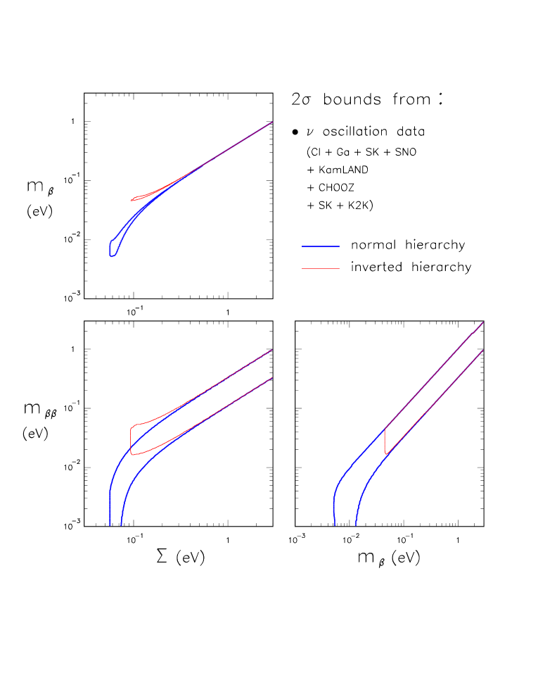
Figure 3: Global $3\nu$ analysis in the $(m_{\beta},m_{\beta\beta},\Sigma)$ parameter space, using oscillation data only. The three panels show the two-dimensional projections of the volume allowed at $\Delta\chi^{2}_{\mathrm{osc}}=4$ ($2\sigma$ on each parameter) for both normal hierarchy (thick solid curves) and inverted hierarchy (thin solid curves), respectively. The emerging correlations between parameters are discussed in the text.

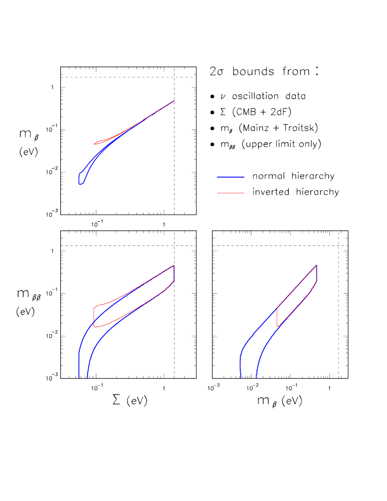
Figure 4: Global $3\nu$ analysis in the $(m_{\beta},m_{\beta\beta},\Sigma)$ parameter space, using oscillation data plus laboratory data and cosmological data. With respect to Fig. 3, this figure implements also upper limits (shown as dashed lines at $2\sigma$ level) on $m_{\beta}$ from Mainz+Troitsk data, on $m_{\beta\beta}$ from $0\nu 2\beta$ data, and on $\Sigma$ from CMB+2dF data. In combination with oscillation parameter bounds, the cosmological upper limit on $\Sigma$ dominates over the laboratory upper limits on $m_{\beta}$ and $m_{\beta\beta}$.

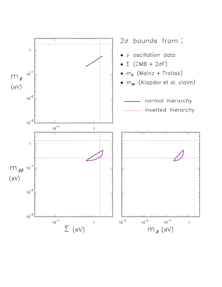
Figure 5: Global $3\nu$ analysis in the $(m_{\beta},m_{\beta\beta},\Sigma)$ parameter space, using oscillation data plus laboratory and cosmological data. With respect to Fig. 4, lower bounds on $m_{\beta\beta}$ from a claimed $0\nu 2\beta$ signal are implemented. The globally allowed $2\sigma$ regions appear to be stretched somewhat beyond the separate $2\sigma$ bands. This feature reflects some tension existing between the $0\nu 2\beta$ claim and cosmological CMB+LSS data within the $3\nu$ oscillation scenario.

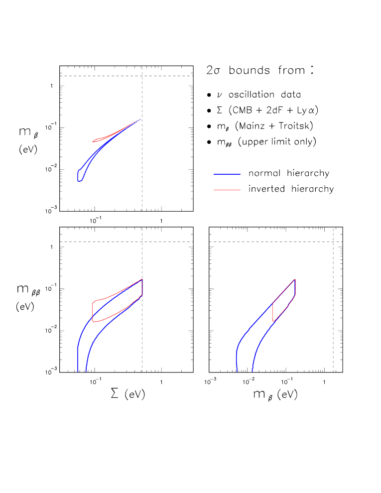
Figure 6: Global $3\nu$ analysis in the $(m_{\beta},m_{\beta\beta},\Sigma)$ parameter space as in Fig. 4, but including Ly$\alpha$ forest data from the SDSS, which lead to a stronger upper bound on $\Sigma$, close to the zone where normal and inverted hierarchies start to branch out in the $(m_{\beta},\Sigma)$ and $(m_{\beta\beta},\Sigma)$ planes.

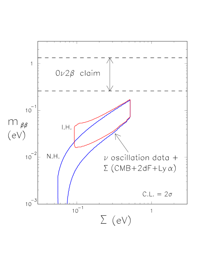
Figure 7: $3\nu$ analysis in the $(m_{\beta\beta},\Sigma)$ plane, showing the absence of overlap between the regions separately allowed at $2\sigma$ by the $0\nu 2\beta$ claim (horizontal band) and by the combination of $\nu$ oscillation data with CMB+2dF+Ly$\alpha$ cosmological data (slanted bands), for both normal hierarchy (N.H.) and inverted hierarchy (I.H.). Such strong tension might indicate possible problems either in some experimental data or in their theoretical interpretation.

- (1) T. Kajita and Y. Totsuka, Rev. Mod. Phys. 73, 85 (2001).
- (2) Super-Kamiokande Collaboration, Y. Ashie et al., Phys. Rev. Lett. 93, 101801 (2004).
- (3) MACRO Collaboration, M. Ambrosio et al., Phys. Lett. B 566, 35 (2003).
- (4) Soudan 2 Collaboration, M. Sanchez et al., Phys. Rev. D 68, 113004 (2003).
- (5) Homestake Collaboration, B.T. Cleveland, T. Daily, R. Davis Jr., J.R. Distel, K. Lande, C.K. Lee, P.S. Wildenhain, and J. Ullman, Astrophys. J. 496, 505 (1998).
- (6) SAGE Collaboration, J.N. Abdurashitov et al., J. Exp. Theor. Phys. 95, 181 (2002) [Zh. Eksp. Teor. Fiz. 95, 211 (2002)].
- (7) T. Kirsten for the GALLEX/GNO Collaboration, in the Proceedings of Neutrino 2002, 20th International Conference on Neutrino Physics and Astrophysics (Munich, Germany, 2002), edited by F. von Feilitzsch and N. Schmitz, Nucl. Phys. B Proc. Suppl. 118, 33 (2003).
- (8) C. Cattadori, “Results from radiochemical solar neutrino experiments,” in Neutrino 2004, 21st International Conference on Neutrino Physics and Astrophysics (Paris, France, 2004); website: neutrino2004.in2p3.fr
- (9) SK Collaboration, S. Fukuda et al., Phys. Rev. Lett. 86, 5651 (2001); Phys. Rev. Lett. 86, 5656 (2001); Phys. Lett. B 539, 179 (2002); M.B. Smy et al., Phys. Rev. D 69, 011104 (2004).
- (10) SNO Collaboration, Q.R. Ahmad et al., Phys. Rev. Lett. 87, 071301 (2001); Phys. Rev. Lett. 89, 011301 (2002); Phys. Rev. Lett. 89, 011302 (2002); S.N. Ahmed et al., Phys. Rev. Lett. 92, 181301 (2004).
- (11) KamLAND Collaboration, K. Eguchi et al., Phys. Rev. Lett. 90, 021802 (2003).
- (12) G. Gratta, “Results from the KamLAND experiment,” in Neutrino 2004 Catt .
- (13) KamLAND Collaboration, T. Araki et al., hep-ex/0406035.
- (14) K2K Collaboration, M.H. Ahn et al., Phys. Rev. Lett. 90, 041801 (2003).
- (15) T. Nakaya, “K2K Results,” in Neutrino 2004 Catt .
- (16) B. Pontecorvo, Zh. Eksp. Teor. Fiz. 53, 1717 (1968) [Sov. Phys. JETP 26, 984 (1968)].
- (17) Z. Maki, M. Nakagawa, and S. Sakata, Prog. Theor. Phys. 28, 870 (1962).
- (18) LSND Collaboration, A. Aguilar et al. Phys. Rev. D 64, 112007 (2001).
- (19) M.C. Gonzalez-Garcia and Y. Nir, Rev. Mod. Phys. 75, 345 (2003).
- (20) V. Barger, D. Marfatia and K. Whisnant, Int. J. Mod. Phys. E 12, 569 (2003).
- (21) R.D. McKeown and P. Vogel, Phys. Rept. 394, 315 (2004).
- (22) G.L. Fogli, E. Lisi, A. Marrone, D. Montanino, A. Palazzo, and A.M. Rotunno, in the electronic Proceedings of PIC 2003, 23rd International Conference on Physics in Collision (Zeuthen, Germany, 2003), eConf C030626: THAT05, 2003 [hep-ph/0310012].
- (23) M. Maltoni, T. Schwetz, M.A. Tortola, and J.W.F. Valle, New J. Phys. 6, 122 (2004).
- (24) S. Goswami, “Global analysis of neutrino oscillations,” in Neutrino 2004 Catt .
- (25) Review of Particle Physics, S. Eidelman et al., Phys. Lett. B 592, 1 (2004).
- (26) See also the review by B. Kayser in PDG4 .
- (27) G. L. Fogli, E. Lisi, D. Montanino, and A. Palazzo, Phys. Rev. D 65, 073008 (2002).
- (28) CHOOZ Collaboration, M. Apollonio et al. Phys. Lett. B 466, 415 (1999); Eur. Phys. J. C 27, 331 (2003).
- (29) E. Holzschuh, Rept. Prog. Phys. 55, 1035 (1992).
- (30) C. Weinheimer, in the Proceedings of the International School of Physics Enrico Fermi, Course 152: Neutrino Physics (Varenna, Lake Como, Italy, 2002), hep-ex/0210050.
- (31) S.M. Bilenky, C. Giunti, J.A. Grifols and E. Masso, Phys. Rept. 379, 69 (2003).
- (32) M. Doi, T. Kotani and E. Takasugi, Prog. Theor. Phys. Suppl. 83, 1 (1985).
- (33) S.R. Elliott and P. Vogel, Ann. Rev. Nucl. Part. Sci. 52, 115 (2002).
- (34) S.R. Elliott and J. Engel, J. Phys. G 30, R183 (2004).
- (35) B.H.J. McKellar, Phys. Lett. B 97, 93 (1980); F. Vissani, in the Proceedings of NOW 2000, Europhysics Neutrino Oscillation Workshop (Conca Specchiulla, Otranto, Italy, 2000), ed. by G.L. Fogli, Nucl. Phys. B (Proc. Suppl.) 100, 273 (2001); J. Studnik and M. Zralek, hep-ph/0110232. See also the discussion in Y. Farzan and A.Yu. Smirnov, Phys. Lett. B 557, 224 (2003).
- (36) C. Weinheimer, in the Proceedings of Neutrino 2002 GALL , p. 279.
- (37) V.M. Lobashev, in the Proceedings of NPDC 17, 17th International Nuclear Physics Divisional Conference: Europhysics Conference on Nuclear Physics in Astrophysics (Debrecen, Hungary, 2002), ed. by N. Auerbach, Zs. Fulop, Gy. Gyurky, and E. Somorjai, Nucl. Phys. A 719, 153 (2003).
- (38) K. Eitel, “Direct Neutrino Mass Experiments,” in Neutrino 2004 Catt .
- (39) L. Wolfenstein, Phys. Lett. B 107, 77 (1981).
- (40) S.M. Bilenky and S.T. Petcov, Rev. Mod. Phys. 59, 671 (1987).
- (41) S.M. Bilenky, J. Hosek, and S.T. Petcov, Phys. Lett. B 94, 495 (1980); J. Schechter and J.W.F. Valle, Phys. Rev. D 22, 2227 (1980).
- (42) H.V. Klapdor-Kleingrothaus, A. Dietz, H.L. Harney, and I.V. Krivosheina, Mod. Phys. Lett. A 16, 2409 (2001).
- (43) H.V. Klapdor-Kleingrothaus, A. Dietz, I.V. Krivosheina, and O. Chkvorets, Nucl. Instrum. Meth. A 522, 371 (2004).
- (44) H.V. Klapdor-Kleingrothaus, I.V. Krivosheina, A. Dietz, and O. Chkvorets, Phys. Lett. B 586, 198 (2004).
- (45) A.D. Dolgov, Phys. Rept. 370, 333 (2002).
- (46) WMAP Collaboration, C.L. Bennett et al., Astrophys. J. Suppl. 148, 1 (2003).
- (47) SDSS Collaboration, M. Tegmark et al., Phys. Rev. D 69, 103501 (2004).
- (48) See also O. Lahav, “Massive Neutrinos and Cosmology,” in Neutrino 2004 Catt .
- (49) W. Hu, D.J. Eisenstein, and M. Tegmark, Phys. Rev. Lett. 80, 5255 (1998).
- (50) C.P. Ma and E. Bertschinger, Astrophys. J. 455, 7 (1995).
- (51) SDSS Collaboration, P. McDonald et al., astro-ph/0405013.
- (52) U. Seljak et al., astro-ph/0407372.
- (53) An incomplete list includes: F. Vissani, JHEP 9906, 022 (1999); S. M. Bilenky, S. Pascoli, and S.T. Petcov, Phys. Rev. D 64, 053010 (2001); H.V. Klapdor-Kleingrothaus, H. Päs, and A.Yu. Smirnov, Phys. Rev. D 63, 073005 (2001); W. Rodejohan, Nucl. Phys. B 597, 110 (2001); M. Czakon, J. Gluza, J. Studnik, and M. Zralek, Phys. Rev. D 65, 053008 (2002); F. Feruglio, A. Strumia, and F. Vissani, Nucl. Phys. B 637, 345 (2002) [Addendum-ibid. B 659, 359 (2003); S. Pascoli, S.T. Petcov, and L. Wolfenstein, Phys. Lett. B 524, 319 (2002) 359 (2003)]; S. Pascoli and S.T. Petcov, Phys. Lett. B 544, 239 (2002); H. Nunokawa, W.J.C. Teves, and R. Zukanovich Funchal, Phys. Rev. D 66, 093010 (2002); F.R. Joaquim, Phys. Rev. D 68, 033019 (2003); S. Pascoli, S.T. Petcov, and W. Rodejohann, Phys. Lett. B 558, 141 (2003).
- (54) S.M. Bilenky, A. Faessler, and F. Simkovic, Phys. Rev. D 70, 033003 (2004).
- (55) G.L. Fogli, E. Lisi, A. Marrone, D. Montanino, and A. Palazzo, Phys. Rev. D 66, 053010 (2002); G.L. Fogli, G. Lettera, E. Lisi, A. Marrone, A. Palazzo, and A. Rotunno, Phys. Rev. D 66, 093008 (2002); G.L. Fogli, E. Lisi, A. Marrone, D. Montanino, A. Palazzo, and A.M. Rotunno, Phys. Rev. D 67, 073002 (2003); G.L. Fogli, E. Lisi, A. Marrone, and D. Montanino, Phys. Rev. D 67, 093006 (2003).
- (56) G.L. Fogli, E. Lisi, A. Marrone, D. Montanino, A. Palazzo, and A.M. Rotunno, Phys. Rev. D 69, 017301 (2004).
- (57) S. Gardner, V. Bernard, and U.G. Meissner, Phys. Lett. B 598, 188 (2004).
- (58) H.V. Klapdor-Kleingrothaus et al., Eur. Phys. J. A 12, 147 (2001).
- (59) O. Civitarese and J. Suhonen, Nucl. Phys. A 729, 867 (2003).
- (60) J.N. Bahcall, H. Murayama, and C. Peña-Garay, Phys. Rev. D 70, 033012 (2004).
- (61) F. Simkovic, G. Pantis, J.D. Vergados and A. Faessler, Phys. Rev. C 60, 055502 (1999).
- (62) M. Aunola and J. Suhonen, Nucl. Phys. A 643, 207 (1998).
- (63) V.A. Rodin, A. Faessler, F. Simkovic, and P. Vogel, Phys. Rev. C 68, 044302 (2003).
- (64) G. D’Agostini, physics/0403086. The homepage www-zeus.roma1.infn.it/∼dagos also contains extensive references to statistical issues in physics.
- (65) R. Bean and A. Melchiorri, Phys. Rev. D 65, 041302 (2002).
- (66) W. Freedman et al., Astrophys. J. 553, 47 (2001).
- (67) J. Dunkley et al., astro-ph/0405462.
- (68) R. Durrer et al., Phys. Rev. D 59, 123005 (1999).
- (69) J. Lesgourgues, S. Pastor, and L. Perotto, Phys. Rev. D 70, 045016 (2004).
- (70) R. Bowen et al., Mon. Not. Roy. Astron. Soc. 334, 760 (2002).
- (71) L. Verde et al., Astrophys. J. Suppl. 148, 195 (2003).
- (72) See the website: lambda.gsfc.nas.gov/index.cfm
- (73) BOOMERanG Collaboration, J.E. Ruhl et al., Astrophys. J. 599, 786 (2003).
- (74) N.W. Halverson et al., Astrophys. J. 568, 38 (2002).
- (75) A.T. Lee et al., Astrophys. J. 561, L1 (2001).
- (76) A.C.S. Readhead et al., Astrophys. J. 609, 498 (2004).
- (77) C. Dickinson et al., astro-ph/0402498.
- (78) A. Melchiorri and J. Silk, Phys. Rev. D 66, 041301 (2002).
- (79) W.J. Percival et al., Mon. Not. Roy. Astron. Soc. 327, 1297 (2001).
- (80) Supernova Search Team Collaboration, A.G. Riess et al., Astrophys. J. 607, 665 (2004).
- (81) S. Hannestad, JCAP 0305, 004 (2003).
- (82) V. Barger, D. Marfatia, and A. Tregre, Phys. Lett. B 595, 55 (2004).
- (83) P. Crotty, J. Lesgourgues, and S. Pastor, Phys. Rev. D 69, 123007 (2004).
- (84) A. Blanchard, M. Douspis, M. Rowan-Robinson, and S. Sarkar, Astron. Astrophys. 412, 35 (2003).
- (85) V.D. Barger and K. Whisnant, Phys. Lett. B 456, 194 (1999).
- (86) V. Barger, S.L. Glashow, D. Marfatia, and K. Whisnant, Phys. Lett. B 532, 15 (2002).
- (87) K. Matsuda, N. Takeda, T. Fukuyama, and H. Nishiura, Phys. Rev. D 64, 013001 (2001).
- (88) See, e.g., the talks by Y. Suzuki, H. Gallagher, T. Kobayashi, and M. Mezzetto in Neutrino 2004 Catt .
- (89) See, e.g., the talks by Y. Hayato, L. Oberauer, and M. Messier in Neutrino 2004 Catt .
- (90) See, e.g., the talk by A. Blondel in Neutrino 2004 Catt .
- (91) F. Avignone, “Strategy for future double beta experiments,” in Neutrino 2004 Catt .