Abstract

Gauge fields and both adjoint and fundamental Higgs fields are unified in gauge theory defined on an orbifold. It is shown how the Hosotani mechanism at the quantum level resolves the problem of the arbitrariness in boundary conditions imposed at the fixed points of the orbifold. The role of adjoint Higgs fields in the standard GUT, which are extra-dimensional components of gauge fields in the current scheme, is taken by the Hosotani mechanism and additional dynamics governing the selection of equivalence classes of boundary conditions. The roles of fundamental Higgs fields, namely those of inducing the electroweak symmetry breaking and giving masses to quarks and leptons, are taken by the Hosotani mechanism and by extra twists in boundary conditions for matter. SUSY scenario nicely fits this scheme. Explicit models are given for the gauge groups $U(3)\times U(3)$, $SU(5)$, and $SU(6)$ on the orbifolds $M^{4}\times(S^{1}/Z_{2})$ and $M^{4}\times(T^{2}/Z_{2})$.

31 July 2004 OU-HET 477/2004

(No. 12-0068)

Yutaka Hosotani

Department of Physics, Osaka University, Toyonaka, Osaka 560-0043, Japan

1.  Introduction

Gauge theory in higher dimensions, particularly gauge theory on orbifolds, has been studied extensively in hoping to resolve the long-standing problems in grand unified theory (GUT) such as the gauge hierarchy problem, the doublet-triplet splitting problem, and the origin of gauge symmetry breaking.[1]-[5] One intriguing aspect is the gauge-Higgs unification in which Higgs bosons are regarded as a part of extra-dimensional components of gauge fields.[6]-[15]

When extra-dimensional space is not simply connected, dynamical gauge symmetry breaking can occurs through the Hosotani mechanism, gauge symmetry breaking by the Wilson lines.[7, 8] Extra-dimensional components of gauge fields (Wilson line phases) become dynamical degrees of freedom, which cannot be gauged away. They, in general circumstances, develop nonvanishing vacuum expectation values. Extra-dimensional components of gauge fields act as Higgs bosons at low energies. Thus gauge fields and Higgs particles are unified through higher dimensional gauge invariance. One does not need to introduce extra Higgs fields to break the gauge symmetry. The gauge invariance also protects Higgs fields from aquiring large masses by radiative corrections.

To construct realistic GUT or unified electroweak theory, one can choose extra dimensions to be an orbifold. By having an orbifold in extra dimensions, one can accommodate chiral fermions in four dimensions, and also rich patterns of gauge symmetry breaking. In this paper we discuss gauge theory on $M^{4}\times(S^{1}/Z_{2})$ and $M^{4}\times(T^{2}/Z_{2})$.

2.  Gauge-Higgs unification

The idea of unifying Higgs scalar fields with gauge fields was first proposed by Manton and Fairlie[6]. Manton considered $SU(3)$ or $G_{2}$ gauge theory on $M^{4}\times S^{2}$. He, in ad hoc way, supposed that field strengths on $S^{2}$ are nonvanishing in such a way that gauge symmetry breaks down to the electroweak $SU(2)_{L}\times U(1)_{Y}$. Extra-dimensional components of gauge fields of the broken part are the Weinberg-Salam Higgs fields. One of the serious problems in this senario is the fact that the configuration with nonvanishing field strengths has higher energy density than the trivial configration with vanishing field strengths so that it will decay. The stability is not guaranteed even if the $S^{2}$ topology of the extra-dimnsional space is maintained for other causes.

There is a natural way of implementing the gauge-Higgs unification. In 1983 it was shown that in gauge theory defined on non-simply connected space, dynamics of Wilson line phases can induce gauge symmetry breaking. Particularly it was proposed there that adjoint Higgs fields in GUT are extra-dimensional components of gauge fields. Dynamical symmetry breaking $SU(5)\rightarrow SU(3)\times SU(2)\times U(1)$ can take place at the quantum level by the Hosotani mechanism.[7]

Recently it has been found that in gauge theory defined on orbifolds boundary conditions at fixed points on orbifolds can implement gauge symmetry breaking. It is subsequently pointed out that different sets of boundary conditions can be physically equivalent through the Hosotani mechanism. Consequently quantum treatment of Wilson line phases becomes crucial to determine the physical symmetry of the theory.[13]

Before going into the details, we stress that there are two types of gauge-Higgs unification.

(i) Gauge-adjoint-Higgs unification

In most of grand unified theories (GUT), Higgs fields in the adjoint representation are responsible for inducing gauge symmetry breaking down to the standard model symmetry, $SU(3)\times SU(2)\times U(1)$. The expectation value of such Higgs fields is typically of O($M_{\rm GUT}$). In higher dimensional gauge theory extra-dimensional components of gauge fields can serve as Higgs fields in the adjoint representation in four dimensions at low energies. This is called gauge-adjoint-Higgs unification. It was first introduced in ref. [7].

(ii) Gauge-fundamental-Higgs unification

Electroweak symmetry breaking is induced by Higgs fields in the fundamental representation. In the Weinberg-Salam theory they are $SU(2)_{L}$ doublets. In the $SU(5)$ GUT they are in the 5 representation. Higgs fields in the fundamental representation have another important role of giving fermions finite masses.

To unify a scalar field in the fundamental representation with gauge fields, the gauge group has to be enlarged, as the scalar field need to become a part of gauge fields. In Manton’s approach,[6] the gauge group is $SU(3)$ or $G_{2}$. In GUT one can start with $SU(6)$ which breaks to $SU(3)\times SU(2)\times U(1)^{2}$.

3.  Gauge theory on non-simply connected manifolds and orbifolds

If the space is non-simply connected, Wilson line phases become physical degrees of freedom. Although constant Wilson line phases yield vanishing field strengths, they are dynamical and affect physics. At the classical level Wilson line phases label degenerate vacua. The degeneracy is lifted by quantum effects. The effective potential of Wilson line phases become non-trivial. Wilson line phases are non-Abelian Aharonov-Bohm phases. If the effective potential is minimized at nontrivial values of Wilson line phases, then the rearrangement of gauge symmetry takes place. Spontaneous gauge symmetry breaking or enhancement is achieved dynamically.

A class of orbifolds are obtained by dividing non-simply connected manifolds by discrete symmetry. Examples are $S^{1}/Z_{2}$ and $T^{2}/Z_{n}$. In the course of this “orbifolding” there appear fixed points under the discrete symmetry operation. Theory requires additional boundary conditions at those fixed points. It gives us benefit of eliminating some of light modes in various fields. Chiral fermions naturally appears at low energies. Some of Wilson line phases drops out from the spectrum, while the others survive. The surviving Wilson line phases can dynamically alter the boundary conditions at the fixed points and the physical symmetry of the theory.

Let us take an example. First consider $SU(N)$ gauge theory on $M^{4}\times T^{n}$. $x^{\mu}$ ($\mu=0,\cdots,3$) and $y^{a}$ $(a=1,\cdots,n)$ are coordinates of $M^{4}$ and $T^{n}$, respectively. Loop translation along the $a$-th axis on $T^{n}$ gives

$$T_{a} : \vec{y}+\vec{l}_{a}~{}\sim~{}\vec{y}$$ (3.2)

$$\vec{l}_{a}=(0,\cdots,2\pi R_{a},\cdots,0)~{}~{}~{}(a=1,2,\cdots,n)~{}.$$

Although $(x,\vec{y})$ and $(x,\vec{y}+\vec{l}_{a})$ represent the same point on $T^{n}$, the values of fields need not be the same. In general

$$\hskip-28.45274ptA_{M}(x,\vec{y}+\vec{l}_{a})=U_{a}A_{M}(x,\vec{y})\,U_{a}^{\dagger}~{}~{}~{},$$ (3.3)

$$\hskip-28.45274pt\psi(x,\vec{y}+\vec{l}_{a})=\eta_{a}\,T[U_{a}]\psi(x,\vec{y})~{}~{}~{},$$ (3.4)

$$\hskip-28.45274pt[U_{a},U_{b}]=0~{}~{}~{},~{}~{}~{}U_{a}\in SU(N)~{}~{}~{}(a,b=1,\cdots,n)~{}.$$ (3.5)

$\eta_{a}$ is a $U(1)$ phase factor. $T[U_{a}]\psi=U_{a}\psi$ or $U_{a}\psi U_{a}^{\dagger}$ for $\psi$ in the fundamental or adjoint representation, respectively. The boundary condition (3.5) guanrantees that the physics is the same at $(x,\vec{y})$ and $(x,\vec{y}+\vec{l}_{a})$. The condition $[U_{a},U_{b}]=0$ is necessary to ensure $T_{a}T_{b}=T_{b}T_{a}$. The theory is defined with a set of boundary conditions $\{U_{a},\eta_{a}\}$.

Similar construction is done for gauge theory on orbifolds. Take $M^{4}\times(T^{n}/Z_{2})$ as an example. $Z_{2}$ orbifolding gives

$$Z_{2}~{}:~{}-\vec{y}~{}\sim~{}\vec{y}~{}~{}~{}.$$ (3.6)

Applied on $T^{n}$, this parity operation allows a fixed point $z$ where the relation $\vec{z}=-\vec{z}+\sum_{a}m_{a}\vec{l}_{a}$ ($m_{a}=$ an integer) is satisfied. There appear $2^{n}$ fixed points on $T^{n}$. Combining it with loop translations $T_{a}$ in (3.2), one finds that parity around each fixed point is also a symmetry:

$$Z_{2,j}~{}:~{}\vec{z}_{j}-\vec{y}~{}\sim~{}\vec{z}_{j}+\vec{y}\quad(j=0,\cdots,2^{n}-1)~{}~{}~{}.$$ (3.7)

Accordingly fields must satisfy additional boundary conditions. To be definite, let spacetime be $M^{4}\times(T^{2}/Z_{2})$, in which case $\vec{z}_{0}=(0,0)$, $\vec{z}_{1}=(\pi R_{1},0)$, $\vec{z}_{2}=(0,\pi R_{2})$, and $\vec{z}_{3}=(\pi R_{1},\pi R_{2})$.

Under $Z_{2,j}$ in (3.7)

$$\hskip-28.45274pt\pmatrix{A_{\mu}\cr A_{y^{a}}\cr}(x,\vec{z}_{j}-\vec{y})=P_{j}\pmatrix{A_{\mu}\cr-A_{y^{a}}\cr}(x,\vec{z}_{j}+\vec{y})\,P_{i}^{\dagger}~{}~{},$$ (3.8)

$$\hskip-28.45274pt\psi(x,\vec{z}_{j}-\vec{y})=\eta_{j}^{\prime}\,T[P_{j}]\,(i\Gamma^{4}\Gamma^{5})\psi(x,\vec{z}_{j}+\vec{y})\qquad(\eta_{j}^{\prime}=\pm 1)$$ (3.9)

$$\hskip-28.45274pt\qquad(a=1,2,\quad j=0,1,2,3)~{}~{}.$$ (3.10)

Here $P_{j}=P_{j}^{-1}=P_{j}^{\dagger}\in SU(N)$. Not all $U_{a}$’s and $P_{j}$’s are independent. On $T^{2}/Z_{2}$, only three of them are independent. One can show that

$$\hskip-28.45274ptU_{a}=P_{a}P_{0}~{}~{}~{},~{}~{}~{}P_{3}=P_{2}P_{0}P_{1}=P_{1}P_{0}P_{2}~{}~{}~{},$$ (3.11)

$$\hskip-28.45274pt\eta_{a}=\eta_{0}^{\prime}\eta_{a}^{\prime}=\pm 1\quad(a=1,2)~{}.$$ (3.12)

Gauge theory on $M^{4}\times(T^{2}/Z_{2})$ is specified with a set of boundary conditions $\{P_{j},\eta_{j}^{\prime}~{};~{}j=0,1,2\}$. If fermions $\psi$ in (3.10) are 6-D Weyl fermions, i.e. $\Gamma^{7}\psi=+\psi$ or $-\psi$ where $\Gamma^{7}=\Gamma^{0}\cdots\Gamma^{5}$, then the boundary condition (3.10) makes 4D fermions chiral.

At a first look, the original gauge symmetry is broken by the boundary conditions if $P_{0}$, $P_{1}$ and $P_{2}$ are not proportional to the identity matrix. This part of the symmetry breaking is often called the orbifold symmetry breaking in the literature. As we see below, however, the physical symmetry of the theory can be different from the symmetry of the boundary conditions, and different sets of boundary conditions can be equivalent to each other.

4.  Wilson line phases and the Hosotani mechanism

It is important to recognize that sets of boundary conditions form equivalence classes. Under a gauge transformation

$$A_{M}^{\prime}=\Omega\bigg{(}A_{M}-{i\over g}\partial_{M}\bigg{)}\Omega^{\dagger}$$ (4.1)

$A_{M}^{\prime}$ obeys a new set of boundary conditions $\{P_{j}^{\prime},U_{a}^{\prime}\}$ where

$$\hskip-28.45274ptP_{j}^{\prime}=\Omega(x,\vec{z}_{j}-\vec{y})\,P_{j}\,\Omega(x,\vec{z}_{j}+\vec{y})^{\dagger}~{},$$ (4.2)

$$\hskip-28.45274ptU_{a}^{\prime}=\Omega(x,\vec{y}+\vec{l}_{a})\,U_{a}\,\Omega(x,\vec{y})^{\dagger}~{},$$ (4.3)

$$\hskip 0.0pt\hbox{provided ~{}}\partial_{M}P_{j}^{\prime}=\partial_{M}U_{a}^{\prime}=0~{}~{}.$$ (4.4)

The set $\{P_{j}^{\prime}\}$ can be different from the set $\{P_{j}\}$. When the relations in (4.4) are satisfied, we write

$$\{P_{j}^{\prime}\}~{}\sim~{}\{P_{j}\}~{}~{}.$$ (4.5)

This relation is transitive, and therefore is an equivalence relation. Sets of boundary conditions form equivalence classes of boundary conditions with respect to the equivalence relation (4.5). [8, 13, 16]

The equivalence relation (4.5) indeed implies the equivalence of physics as a result of dynamics of Wilson line phases. Wilson line phases are zero modes ($x$- and $\vec{y}$-independent modes) of extra-dimensional components of gauge fields which satisfy

$$\hskip-28.45274ptA_{y_{a}}=\sum_{\alpha\in H_{W}}\hbox{${1\over 2}$}A_{y_{a}}^{\alpha}\lambda^{\alpha}~{}~{}~{},~{}~{}~{}[A_{y_{a}},A_{y_{b}}]=0~{}~{}~{},~{}~{}~{}(a,b=1,\cdots,n)~{},$$ (4.6)

$$\hskip-28.45274ptH_{W}=\Big{\{}~{}\lambda^{\alpha}~{};~{}\{\lambda^{\alpha},P_{j}\}=0\quad(j=0,\cdots,2^{n}-1)~{}\Big{\}}~{}.$$ (4.7)

Consistency with the boundary condition (3.10) requires $\lambda^{\alpha}$ in the sum to belong to $H_{W}$. Given the boundary conditions, these Wilson line phases cannot be gauged away. They are physical degrees of freedom. They label degenerate classical vacua. To put it differently, Wilson line phases parametrize flat dirrections in the classical potential. The values of $\raise 0.68889pt\hbox{$\langle$}\lower 0.68889pt\hbox{}A_{y_{a}}\,\raise 0.68889pt\hbox{$\rangle$}\lower 0.68889pt\hbox{}$ are determined, at the quantum level, from the location of the absolute minimum of the effective potential $V_{\rm eff}[A_{y_{a}}]$.

Physical symmetry is determined in the combination of the boundary conditions $\{P_{j},\eta_{j}^{\prime}\}$ and the expectation values of the Wilson line phases $\raise 0.68889pt\hbox{$\langle$}\lower 0.68889pt\hbox{}A_{y_{a}}\,\raise 0.68889pt\hbox{$\rangle$}\lower 0.68889pt\hbox{}$. Physical symmetry is, in general, different from the symmetry of the boundary conditions. As a result of quantum dynamics gauge symmetry can be dynamically broken by Wilson line phases.

This is called the Hosotani mechanism. The mechanism on non-simply connected manifolds was put forward in ref. [7]. The importance of equivalence classes of boundary conditions was clarified in ref. [8]. The detailed analysis of the Hosotani mechanism in gauge theory on orbifolds was given in ref. [13]. The mechanism is summarized as follows.

• Wilson line phases, $\theta_{W}$, are physical degrees of freedom and specify degenerate classical vacua.

• Quantum effects lift the degeneracy. The effective potential for the Wilson line phases $V_{\rm eff}[\theta_{W}]$ is nontrivial at the quantum level. The global minimum of $V_{\rm eff}[\theta_{W}]$ determines the physical vacuum.

• If $V_{\rm eff}[\theta_{W}]$ is minimized at nontrivial $\theta_{W}$, gauge symmetry is spontaneously broken or enhanced.

• Gauge fields and adjoint Higgs fields (zero modes of $A_{y}$) are unified.

• Adjoint Higgs fields acquire finite masses at the one loop level. Finiteness of the masses is guaranteed by the gauge invariance.

• Physics is the same within each equivalence class of boundary conditions. It does not depend on sets of boundary conditions to start with so long as they belong to the same equivalence class.

• Physical symmetry of theory is determined by matter content.

In the mechanism Higgs fields are naturally identified with extra-dimensional components of gauge fields. The expectation values of Higgs fields are determined dynamically. It is dynamical gauge-Higgs unification.

5.  $SU(N)$ gauge theory on $M^{4}\times T^{n}$

On a torus $T^{n}$ the boundary conditions are given by (3.5), denoted by $\{U_{a}~{}(a=1,\cdots,n)\}$. Making use of the commutativity relations $U_{a}U_{b}=U_{b}U_{a}$, one can show that

$$\{~{}U_{a}~{}\}~{}\sim~{}\{~{}I~{}\}~{}~{}.$$ (5.1)

In other words, there is only one equivalence class. Physics does not depend on $\{U_{a}~{}(a=1,\cdots,n)\}$. In particular, in pure gauge theory the gauge symmetry remains unbroken even if nontrivial $U_{a}\in SU(N)$ are imposed.

6.  $SU(5)$ GUT on $M^{4}\times(S^{1}/Z_{2})$

Kawamura pointed out that in $SU(5)$ gauge theory on $M^{4}\times(S^{1}/Z_{2})$ with the boundary conditions

$${\rm BC}_{1}~{}:~{}~{}P_{0}=\pmatrix{1\cr&1\cr&&1\cr&&&1\cr&&&&1\cr}~{}~{}~{},~{}~{}~{}P_{1}=\pmatrix{1\cr&1\cr&&1\cr&&&-1\cr&&&&-1\cr}~{}~{}~{},$$ (6.1)

the triple-doublet Higgs mass splitting problem can be naturally solved.[4] In his model there are no Wilson line phases surviving. $SU(5)$ symmetry is broken to $SU(3)\times SU(2)\times U(1)$ by boundary conditions, and there are no colored Higgs triplets to begin with.

A question arises about the choice of boundary conditions to be imposed. Why do one need to choose BC₁? This problem is called as the arbitrariness problem of boundary conditions.[14] It is known that in $SU(N)$ gauge theory on $M^{4}\times(S^{1}/Z_{2})$, there are $(N+1)^{2}$ equivalence classes of boundary conditions.[16]

One can start with

$${\rm BC}_{2}~{}:~{}~{}P_{0}=P_{1}=\pmatrix{1\cr&1\cr&&1\cr&&&-1\cr&&&&-1\cr}~{}~{}~{},$$ (6.2)

or more generally

$${\rm BC}_{3} : P_{0}=\pmatrix{1\cr&1\cr&&1\cr&&&-1\cr&&&&-1\cr}~{}~{}~{},$$ (6.4)

$$P_{1}=\pmatrix{\cos\alpha&0&0&i\sin\alpha&0\cr 0&\cos\beta&0&0&i\sin\beta\cr 0&0&1&0&0\cr-i\sin\alpha&0&0&-\cos\alpha&0\cr 0&-i\sin\beta&0&0&-\cos\beta\cr}~{}~{}~{}.$$

BC₂ is a special case of BC₃ with $\alpha=\beta=0$. The detailed analysis of the theory with BC₃ was given in ref. [13].

Note first that BC₂ and BC₃ belong to the same equivalence class:

$${\rm BC}_{2}~{}\sim~{}{\rm BC}_{3}~{}~{}~{}.$$ (6.5)

Symmetry of boundary conditions, however, depends on $\alpha$ and $\beta$:

$$\hbox{symmetry of BC}~{}=~{}\cases{SU(3)\times SU(2)\times U(1)&for $(\alpha,\beta)=(0,0)$\cr\kern 3.0pt\cr SU(2)\times U(1)^{3}&for $(\alpha,\beta)=(\pi,0),(0,\pi)$\cr\kern 3.0pt\cr SU(2)^{2}\times U(1)^{2}&for $(\alpha,\beta)=(\pi,\pi)$\cr\kern 3.0pt\cr U(1)^{3}&otherwise.\cr}$$ (6.6)

The Hosotani mechanism tells us that once matter content in the theory is specified, physical symmetry is uniquely determined. It is of great interest to know if $SU(3)\times SU(2)\times U(1)$ symmetry remains intact in supersymmetric $SU(5)$ theory.

To determine the physical vacuum, one need to evaluate the effective potential for the Wilson line phases.[11, 13, 19, 20] With the aid of gauge invariance, it suffices to evaluate the effective potential in the theory with any values of $(\alpha,\beta)$ in BC₃. Take $(\alpha,\beta)=(0,0)$, or BC₂. Wilson line phases are the components of $A_{y}$ marked with $\star$ in

$$A_{y}=\pmatrix{&&&\star&\star\cr&&&\star&\star\cr&&&\star&\star\cr\star&\star&\star\cr\star&\star&\star\cr}~{}~{}.$$ (6.7)

Employing the residual $SU(3)\times SU(2)\times U(1)$ symmetry of boundary conditions, one can reduce it to

$$2gRA_{y}=\pmatrix{&&&a\cr&&&&b\cr&&&\cr a\cr&b\cr}~{}~{}.$$ (6.8)

$a$ and $b$ are phases with a normalized period 2.

We consider supersymmetric $SU(5)$ model with $N_{h}$ Higgs scalar fields in 5 representation. We suppose that quarks and leptons are localized on the brane at one of the fixed points on $S^{1}/Z_{2}$. Supersymmetry breaking is introduced by Scherk-Schwarz $SU(2)_{R}$ twist. The Scherk-Schwarz phase is denoted by $\beta$. Then the effective potential becomes

$$\hskip-42.67912ptV_{\rm eff}(a,b)=-{3\over 32\pi^{7}R^{5}}\sum_{n=1}^{\infty}{1\over n^{5}}(1-\cos 2\pi n\beta)~{}\bigg{\{}2(1-N_{h})(\cos\pi na+\cos\pi nb)$$ (6.9)

$$\hskip 113.81102pt+4\cos\pi na\cos\pi nb+\cos 2\pi na+\cos 2\pi nb\bigg{\}}~{}.$$ (6.10)

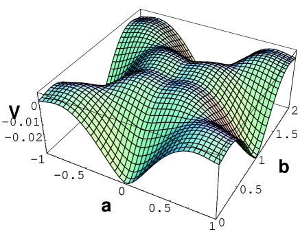
In the minimal model, $N_{h}=1$. As displayed in fig. 1, $V_{\rm eff}(a,b)$ is minimized at $(a,b)=(0,0)$ and $(1,1)$. Physical symmetry at $(a,b)=(0,0)$ is $SU(3)\times SU(2)\times U(1)$, whereas $SU(2)\times SU(2)\times U(1)\times U(1)$ at $(a,b)=(1,1)$. In the minimal supersymmetric model these two phases are degenerate. For $N_{h}\geq 2$, $(a,b)=(1,1)$ is the global minimum. One sees that the standard model symmetry can be obtained only for $N_{h}\leq 1$.

Figure 1: $(32\pi^{7}R^{5}/3)V_{\rm eff}(a,b)$ in (6.10) for $N_{h}=1$ and $\beta=0.1$ is depicted. For $N_{h}=1$ there are degenerate global minima at $(0,0)$ and $(1,1)$.

In this model $M_{\rm GUT}\sim 1/R$. Supersymmetry breaking scale is given by $M_{\rm SUSY}\sim\beta/R\sim\beta M_{\rm GUT}$. Adjoint Higgs bosons ($A_{y}$ in $H_{W}$) acquire masses of $g_{4}M_{\rm SUSY}$ where $g_{4}$ is the four-dimensional gauge coupling.

7.  $U(3)_{S}\times U(3)_{W}$ model on $M^{4}\times(T^{2}/Z_{2})$

In the $SU(5)$ model described above, the Higgs fields in the fundamental representation are not unified. To achieve the gauge-fundamental-Higgs unification one has to enlarge the gauge group such that fundamental Higgs fields in group $G$ can be identified with a part of gauge fields in the enlarged group $\hat{G}$.

The original proposal by Manton was along this line, but the resultant low energy theory was far from the reality. One interesting model was proposed by Antoniadis, Benakli and Quiros a few years ago.[10] They start with a product of two gauge groups $U(3)_{S}\times U(3)_{W}$ with gauge couplings $g_{S}$ and $g_{W}$. $U(3)_{S}$ is “strong” $U(3)$ which decomposes to color $SU(3)_{c}$ and $U(1)_{3}$. $U(3)_{W}$ is “weak” $U(3)$ which decomposes to weak $SU(3)_{W}$ and $U(1)_{2}$. The theory is defined on $M^{4}\times(T^{2}/Z_{2})$. Boundary conditions at fixed points of $T^{2}/Z_{2}$ are imposed in the following manner. For the $U(3)_{S}$ group, all $P_{0}$, $P_{1}$ and $P_{2}$ are taken to be identity matrix. For $U(3)_{W}$ one takes

$$P_{0}=P_{1}=P_{2}=\pmatrix{-1\cr&-1\cr&&+1\cr}~{}~{}~{}.$$ (7.1)

The boundary condition (7.1) breaks $SU(3)_{W}$ to $SU(2)_{L}\times U(1)_{1}$ at the classical level. There are three $U(1)$’s left over.

Fermions obey boundary condition in (3.10). Let $(n_{S},n_{W})^{\sigma}$ stand for a fermion in the $n_{S}$ ($n_{W}$) representation of $U(3)_{S}$ ($U(3)_{W}$) with 6D-Weyl eigenvalue $\Gamma^{7}=\sigma$. Three generations of leptons are assigned as follows. Leptons are

$$L_{1,2,3}=(1,3)^{+}~{}~{}~{}:~{}~{}~{}\pmatrix{{\nu_{L}}\cr{e_{L}}\cr\tilde{e}_{L}\cr}~{},~{}\pmatrix{\tilde{\nu}_{R}\cr\tilde{e}_{R}\cr{e_{R}}\cr}~{}~{}\hbox{etc}.$$ (7.2)

Similarly, for right-handed down quarks we have

$$D^{c}_{1,2,3}=(\bar{3},1)^{+}~{}~{}~{}:~{}~{}~{}{d^{c}_{L}}~{}~{},~{}~{}{\tilde{d}^{c}_{R}}~{}~{}\hbox{etc}.$$ (7.3)

For other quarks, each generation has its own assignment:

$$Q_{1}=(3,\bar{3})^{+} \pmatrix{{u_{L}}\cr{d_{L}}\cr\tilde{u}_{L}\cr}~{},~{}\pmatrix{\tilde{u}_{R}\cr\tilde{d}_{R}\cr{u_{R}}\cr}$$ (7.4)

$$Q_{2}=(3,\bar{3})^{-} \pmatrix{{c_{L}}\cr{s_{L}}\cr\tilde{c}_{L}\cr}~{},~{}\pmatrix{\tilde{c}_{R}\cr\tilde{s}_{R}\cr{c_{R}}\cr}$$ (7.5)

$$Q_{3}=(\bar{3},3)^{-} \pmatrix{\tilde{t}_{L}^{c}\cr\tilde{b}_{L}^{c}\cr{t_{L}^{c}}\cr}~{},~{}\pmatrix{{t_{R}^{c}}\cr{b_{R}^{c}}\cr\tilde{t}_{R}^{c}\cr}~{}.$$ (7.6)

Due to the boundary conditions either $SU(2)_{L}$ doublet part or singlet part has zero modes. In (7.2)-(7.6), fields with tilde $\tilde{~{}}$ do not have zero modes.

With these assignments of fermions only one combination of three $U(1)$ gauge groups remains anomaly free, which is identified with weak hypercharge $U(1)_{Y}$. Gauge bosons corresponding to the other two combinations of three $U(1)$ gauge groups become massive by the Green-Schwarz mechanism. Hence, the remaining symmetry at this level is $SU(3)_{c}\times SU(2)_{L}\times U(1)_{Y}$.

There are Wilson line phases in the $SU(3)_{W}$ group. They are

$$A_{y_{1}}=\pmatrix{&&\star\cr&&\star\cr\star&\star\cr}=\pmatrix{~{}&{\vphantom{{\displaystyle 1\over\displaystyle 2}}}\Phi_{1}\cr~{}~{}\Phi_{1}^{\dagger}~{}&\cr}~{}~{},~{}~{}A_{y_{2}}=\pmatrix{~{}&{\vphantom{{\displaystyle 1\over\displaystyle 2}}}\Phi_{2}\cr~{}~{}\Phi_{2}^{\dagger}~{}&\cr}~{}~{}.$$ (7.7)

$\Phi_{1}$ and $\Phi_{2}$ are $SU(2)_{L}$ doublets. The resultant theory is the Weinberg-Salam theory with two Higgs doublets. The classical potential for the Higgs fields results from the $F_{y_{1}y_{2}}^{2}$ part of the gauge field action:

$$V_{\rm tree}(\Phi_{1},\Phi_{2})=g_{W}^{2}\Big{\{}\Phi_{1}^{\dagger}\Phi_{1}\cdot\Phi_{2}^{\dagger}\Phi_{2}+\Phi_{2}^{\dagger}\Phi_{1}\cdot\Phi_{1}^{\dagger}\Phi_{2}-(\Phi_{2}^{\dagger}\Phi_{1})^{2}-(\Phi_{1}^{\dagger}\Phi_{2})^{2}\Big{\}}~{}~{}.$$ (7.8)

There is no quadratic term. The potential (7.8) is positive definite and has flat directions. The potential vanishes if $\Phi_{1}$ and $\Phi_{2}$ are proportional to each other with a real proportionality constant.

To determine if the electroweak symmetry is dynamically broken, one need to evaluate quantum corrections to the effective potential of $\Phi_{1}$ and $\Phi_{2}$. The detailed analysis is given in ref. [18]. The effective potential in the flat directions is obtained, without loss of generality, for the configuration

$$2g_{W}R_{1}A_{y_{1}}=\pmatrix{&&0\cr&&a\cr 0&a\cr}~{}~{},~{}~{}2g_{W}R_{2}A_{y_{2}}=\pmatrix{&&0\cr&&b\cr 0&b\cr}~{}~{},$$ (7.9)

where $a$ and $b$ are real. Our task is to find $V_{\rm eff}(a,b)$ and thereby determine the physical vacuum.

Depending on the location of the global minimum of $V_{\rm eff}(a,b)$, the physical symmetry varies. It is given by

$$(a,b)=\cases{(0,0)&$SU(2)_{L}\times U(1)_{Y}$\cr\kern 5.0pt\cr(0,1),(1,0),(1,1)~{}~{}~{}&$U(1)_{EM}\times U(1)_{Z}$\cr\kern 5.0pt\cr\hbox{otherwise}&$U(1)_{EM}$.\cr}$$ (7.10)

For generic values of $(a,b)$, electroweak symmetry breaking takes place. The Weinberg angle is given by

$$\sin^{2}\theta_{W}={1\over 4+{\displaystyle 2g_{W}^{2}\over\displaystyle 3g_{S}^{2}}}~{}~{},$$ (7.11)

which can be very close to the observed value. The deviation from the value $0.25$ is brought by a small ratio $g_{W}/g_{S}$. We note that in the $SU(3)_{c}\times SU(3)_{W}$ model the Weinberg angle turns out too large.[15]

The evaluation of $V_{\rm eff}(a,b)$ is straightforward. A general method of computations on $T^{2}/Z_{2}$ has been described in ref. [17]. In the non-supersymmetric model the matter content is given by gauge fields (including ghosts) and fermions summarized in (7.2)-(7.6). Only gauge fields in $SU(3)_{W}$ give contributions having the ($a,b$) dependence. The result is

$$\hskip-28.45274ptV_{\rm eff}(a,b)=4\bigg{\{}I(0,0)+2\cdot I\Big{(}{a\over 2},{b\over 2}\Big{)}+I(a,b)\bigg{\}}-3\bigg{\{}14\cdot I(0,0)+16\cdot I\Big{(}{a\over 2},{b\over 2}\Big{)}\bigg{\}}$$ (7.12)

$$\hskip 14.22636pt=-40\cdot I\Big{(}{a\over 2},{b\over 2}\Big{)}+4\cdot I(a,b)+\hbox{const.}$$ (7.13)

where

$$\hskip-28.45274ptI(a,b)=-{1\over 16\pi^{2}}\bigg{\{}{1\over R_{1}^{6}}\sum_{n=1}^{\infty}{\cos 2\pi na\over n^{6}}+{1\over R_{2}^{6}}\sum_{m=1}^{\infty}{\cos 2\pi mb\over m^{6}}$$ (7.14)

$$\hskip 85.35826pt+\sum_{n=1}^{\infty}\sum_{m=1}^{\infty}{2\cos 2\pi na\cos 2\pi mb\over(n^{2}R_{1}^{2}+m^{2}R_{2}^{2})^{3}}\bigg{\}}~{}~{}.$$ (7.15)

In the first equality in (7.13), the first and second terms represents contributions from gauge fields and fermions, respectively.

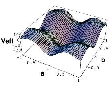
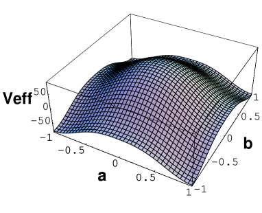
(a) In pure gauge theory.                                    (b) With fermions.

Figure 2: $V_{\rm eff}(a,b)$ in the $U(3)_{S}\times U(3)_{W}$ model.

If there were no fermions, $V_{\rm eff}(a,b)$ has the global minimum at $(a,b)=(0,0)$ so that $SU(2)_{L}\times U(1)_{Y}$ symmetry is unbroken. In the presence of fermions, the point $(a,b)=(0,0)$ becomes unstable. The effective potential (7.13) is displayed in fig. 2. The global minimum is located at $(a,b)=(1,1)$, which corresponds to the $U(1)_{EM}\times U(1)_{Z}$ symmetry. Although the $SU(2)_{L}$ symmetry is partially broken and $W$ bosons acquire masses, $Z$ bosons remain massless.

This result is not what we hoped to obtain. We would like to have a model in which the global minimum of the effective potential is located at non-integral values of $(a,b)$. As Antoniadis et al. mentioned in ref. [10], more general symmetry breaking may occur if one considers a two-torus of general parallelogram. (In this section a rectangular torus has been considered.) More promissing is to incorporate additional fermions, for instance, in the adjoint representation. One can show that such modification indeed yields the global minimum at a generic point.[18]

8.  $SU(6)$ model on $M^{4}\times(S^{1}/Z_{2})$

Gauge-fundamental-Higgs unification can be realized in the framework of GUT as well. To illustrate it, let us consider $SU(6)$ gauge theory on $M^{4}\times(S^{1}/Z_{2})$.[15] We take boundary conditions to be

$$P_{0}=\pmatrix{1\cr&1\cr&&1\cr&&&1\cr&&&&-1\cr&&&&&-1\cr}~{}~{},~{}~{}P_{1}=\pmatrix{1\cr&-1\cr&&-1\cr&&&-1\cr&&&&-1\cr&&&&&-1\cr}~{}~{}.$$ (8.1)

Symmetry of boundary conditions is $SU(3)\times SU(2)\times U(1)^{2}$. Wilson line phases are

$$A_{y}=\pmatrix{0&0&0&0&\star&\star\cr 0\cr 0\cr 0\cr\star\cr\star\cr}=\pmatrix{0&0&0&0&~{}\Phi^{\dagger}~{}~{}\cr 0\cr 0\cr 0\cr{\vphantom{{\displaystyle 1\over\displaystyle 2}}}\Phi\cr}~{}~{}.$$ (8.2)

They serve as a Higgs doublet. Electroweak symmetry breaking is induced if $\Phi$ dynamically develops an expectation value:

$$2gR~{}\raise 0.68889pt\hbox{$\langle$}\lower 0.68889pt\hbox{}\Phi\,\raise 0.68889pt\hbox{$\rangle$}\lower 0.68889pt\hbox{}=\pmatrix{0\cr a\cr}~{}~{}.$$ (8.3)

The effective potential $V_{\rm eff}(a)$ depends on the matter content. On $M^{4}\times(S^{1}/Z_{2})$ fermions satisfy

$$\psi(x,z_{j}-y)=\eta_{j}^{\prime}\,T[P_{j}]\,\Gamma^{5}\psi(x,z_{j}+y)\qquad(\eta_{j}^{\prime}=\pm 1~{},~{}j=0,1)~{}~{}.$$ (8.4)

Here $z_{0}=0$ and $z_{1}=\pi R$. Let $N_{a}^{(+)}$ ($N_{f}^{(-)}$) be the number of fermions in the adjoint (fundamental) representation with $\eta_{0}^{\prime}\eta_{1}^{\prime}=+1$ $(-1)$. Then

$$\hskip 0.0ptV_{\rm eff}(a)={3\over 64\pi^{7}R^{5}}\sum_{n=1}^{\infty}{1\over n^{5}}\bigg{\{}\Big{(}-{3\over 2}+2N_{a}^{(+)}\Big{)}\cos 2\pi na$$ (8.5)

$$\hskip 28.45274pt+\Big{(}-3+4N_{a}^{(+)}\Big{)}\cos\pi na+\Big{(}-9+12N_{a}^{(+)}+2N_{f}^{(-)}\Big{)}\cos\pi n(a-1)\bigg{\}}~{}~{}.$$ (8.6)

When $N_{a}^{(+)}=N_{f}^{(-)}=2$, the global minimum is located at $a=0.072$. From the $W$ boson mass it follows that $a/g_{4}R\sim 246\,$GeV. The mass of the neutral Higgs is found to be

$$m_{H}\sim{0.038g_{4}\over R}\sim 130\,g_{4}^{2}\,\hbox{GeV}~{}.$$ (8.7)

In this senario $1/R$ is at a TeV scale.

The point of this example is to show that it is possible to have a small value for $a$ at the minimum, once one introduces additional fermions.

9.  Summary

We have shown in this paper that dynamical gauge-Higgs unification is achieved in higher dimensional gauge theory. Higgs fields are identified with Wilson line phases in gauge theory. Dynamical symmetry breaking is induced by the Hosotani mechanism.

Boundary conditions which appear in gauge theory on non-simply connected manifolds or orbifolds are classified with equivalence relations. In each equivalence class of boundary conditions physics is the same, as a consequence of quantum dynamics of Wilson line phases.

We have shown that both GUT symmetry breaking and electroweak symmetry breaking can be induced in the present approach. One of the remaining problems is the origin of fermion masses. Fermion masses brought by the Hosotani mechanism are flavor-independent. They depend only on the representation of the group which fermions belong to. There are other origins for fermion masses. There can be additional interactions localized on the boundary brane. We point out that there is a natural origin of fermion masses on $T^{n}/Z_{2}$, namely $T^{n}$ twists for $Z_{2}$ doublets. In the case of fermions on $M^{4}\times(T^{2}/Z_{2})$, we prepare a pair of fermion fields, $(\psi,\hat{\psi})$, and impose, instead of (3.5) and (3.12),

$$\hskip-28.45274pt\pmatrix{\psi\cr\hat{\psi}\cr}(x,-\vec{y})=\eta_{0}^{\prime}\,T[P_{0}]\,(i\Gamma^{4}\Gamma^{5})\pmatrix{\psi\cr-\hat{\psi}\cr}(x,+\vec{y})$$ (9.1)

$$\hskip-28.45274pt\pmatrix{\psi\cr\hat{\psi}\cr}(x,\vec{y}+\vec{l}_{a})=\eta_{a}\,T[U_{a}]\pmatrix{\cos\gamma_{a}&-\sin\gamma_{a}\cr\sin\gamma_{a}&\cos\gamma_{a}\cr}\pmatrix{\psi\cr\hat{\psi}\cr}(x,\vec{y})~{}~{}~{}.$$ (9.2)

This is similar to the Scherk-Schwarz SUSY breaking. If twist parameters $\gamma_{a}$ are small, then the spectrum of light particles at low energies does not change, but light fermions acquire additional small masses of $O(\gamma_{a}/R)$.

Finally we add a comment on the Higgsless model of electroweak interactions recently proposed.[21] The Higgsless model is very similar to Kawamura’s model of $SU(5)$ gauge theory on $M^{4}\times(S^{1}/Z_{2})$.[4] In Kawamura’s model colored triplet Higgs fields are absent due to the boundary conditions. In the Higgsless model boundary conditins are designed such that Higgs doublet fields are absent. In this sense the Higgsless model also belongs to the category of models examined in this paper.

References

[1]
I. Antoniadis, Phys. Lett. B246 (1990) 377;
I. Antoniadis, C. Munoz and M. Quiros, Nucl. Phys. B397 (1993) 515;
[2]
A. Pomarol and M. Quiros, Phys. Lett. B438 (1998) 255.
[3]
H. Hatanaka, T. Inami and C.S. Lim,
Mod. Phys. Lett. A13 (1998) 2601.
[5]
L. Hall and Y. Nomura, Phys. Rev. D64 (2001) 055003;
Ann. Phys. (N.Y.)306 (2003) 132;
R. Barbieri, L. Hall and Y. Nomura,
Phys. Rev. D66 (2002) 045025;
Nucl. Phys. B624 (2002) 63;
M. Quiros, hep-ph/0302189.
[6]
N. Manton, Nucl. Phys. B158 (1979) 141;
D.B. Fairlie, Phys. Lett. B82 (1979) 97; J. Phys. G5 (1979) L55;
P. Forgacs and N. Manton, Comm. Math. Phys. 72 (1980) 15.
[7]
Y. Hosotani, Phys. Lett. B126 (1983) 309.
[8]
Y. Hosotani, Ann. Phys. (N.Y.)190 (1989) 233.
[9]
Y. Hosotani, Phys. Lett. B129 (1984) 193; Phys. Rev. D29 (1984) 731.
[10]
I. Antoniadis, K. Benakli and M. Quiros,
New. J. Phys.3 (2001) 20;
[11]
M. Kubo, C.S. Lim and H. Yamashita,
Mod. Phys. Lett. A17 (2002) 2249.
[12]
G. Dvali, S. Randjbar-Daemi and R. Tabbash,
Phys. Rev. D65 (2002) 064021;
L.J. Hall, Y. Nomura and D. Smith, Nucl. Phys. B639 (2002) 307;
G. Burdman and Y. Nomura, Nucl. Phys. B656 (2003) 3;
C. Csaki, C. Grojean and H. Murayama, Phys. Rev. D67 (2003) 085012;
I. Gogoladze, Y. Mimura and S. Nandi, Phys. Lett. B562 (2003) 307;
Phys. Lett. B560 (2003) 204; hep-ph/0311127;
C.A. Scrucca, M. Serone and L. Silverstrini, Nucl. Phys. B669 (2003) 128;
[13]
N. Haba, M. Harada, Y. Hosotani and Y. Kawamura,
Nucl. Phys. B657 (2003) 169;
Erratum, ibid. B669 (2003) 381. (hep-ph/0212035)
[14]
Y. Hosotani, in ”Strong Coupling Gauge Theories and Effective Field
Theories”, ed. M. Harada, Y. Kikukawa and K. Yamawaki (World Scientific
2003), p. 234. (hep-ph/0303066).
[15]
N. Haba, Y. Hosotani, Y. Kawamura and T. Yamashita,
hep-ph/0401183, to appear in Phys. Rev.D.;
N. Haba and T. Yamashita, hep-ph/0402157.
[16]
N. Haba, Y. Hosotani and Y. Kawamura,
Prog. Theoret. Phys. 111 (2004) 265. (hep-ph/0309088)
[17]
Y. Hosotani, S. Noda, and K. Takenaga,
Phys. Rev. D69 (2004) 125014. (hep-ph/0403106)
[18]
S. Noda, Y. Hosotani, and K. Takenaga, in preparation.
[19]
K. Takenaga, Phys. Lett. B425 (1998) 114;
Phys. Rev. D58 (1998) 026004.
K. Takenaga, Phys. Lett. B570 (2003) 244.
[20]
C.C. Lee and C.L. Ho, Phys. Rev. D62 (2000) 085021;
[21]
C. Csaki, C. Grojean, L. Pilo, and J. Terning,
Phys. Rev. Lett. 92 (2004) 101802;
G. Cacciapaglia, C. Csaki, C. Grojean, and J. Terning,
hep-ph/0401160.