Symmetries of Two Higgs Doublet Model
and CP violation

Abstract

We use the invariance of physical picture under a change of Lagrangian, the reparametrization invariance in the space of Lagrangians and its particular case – the rephrasing invariance, for analysis of the two-Higgs-doublet extension of the SM. We found that some parameters of theory like $\tan\beta$ are reparametrization dependent and therefore cannot be fundamental. We use the $Z_{2}$-symmetry of the Lagrangian, which prevents a $\phi_{1}\leftrightarrow\phi_{2}$ transitions, and the different levels of its violation, soft and hard, to describe the physical content of the model. In general, the broken $Z_{2}$-symmetry allows for a CP violation in the physical Higgs sector. We argue that the 2HDM with a soft breaking of $Z_{2}$-symmetry is a natural model in the description of EWSB. To simplify the analysis we choose among different forms of Lagrangian describing the same physical reality a specific one, in which the vacuum expectation values of both Higgs fields are real.

A possible CP violation in the Higgs sector is described by using a two-step procedure with the first step identical to a diagonalization of the mass matrix for CP-even fields in the CP conserving case. We find very simple necessary and sufficient condition for a CP violation in the Higgs sector. We determine the range of parameters for which CP violation and Flavor Changing Neutral Current effects are naturally small - it corresponds to a small dimensionless mass parameter $\nu=\thinspace{\rm Re\thinspace}m_{12}^{2}/(2v_{1}v_{2})$. We show that for small $\nu$ some Higgs bosons can be heavy, with mass up to about 0.6 TeV, without violating of the unitarity constraints. If $\nu$ is large, all Higgs bosons except one can be arbitrary heavy. We discuss in particular main features of this case, which corresponds for $\nu\rightarrow\infty$ to a decoupling of heavy Higgs bosons.

In the Model II for Yukawa interactions we obtain the set of relations among the couplings to gauge bosons and to fermions which allows to analyse different physical situations (including CP violation) in terms of these very couplings, instead of the parameters of Lagrangian.

I Introduction

A spontaneous electroweak symmetry breaking of $SU(2)\times U(1)$ (EWSB) via the Higgs mechanism is described by the Lagrangian

$${\cal L}={\cal L}^{SM}_{gf}+{\cal L}_{H}+{\cal L}_{Y}\,.$$ (1)

Here, ${\cal L}^{SM}_{gf}$ describes the $SU(2)\times U(1)$ Standard Model interaction of gauge bosons and fermions, ${\cal L}_{H}$ is the Higgs scalar Lagrangian, and ${\cal L}_{Y}$ describes the Yukawa interactions of fermions with Higgs scalars.

In the minimal Standard Model (SM) one scalar isodoublet with hypercharge $Y=1$ is implemented. Here ${\cal L}_{H}=(D_{\mu}\phi)^{\dagger}D_{\mu}\phi-V$, with the Higgs potential $V=\lambda\phi^{4}/2-m^{2}\phi^{2}/2$. A minimum of V describes the vacuum expectation value $v$ as $\langle\phi\rangle=v/\sqrt{2}=\sqrt{m^{2}/2\lambda}$. In this model there is one physical Higgs boson; its couplings to the gauge bosons can be expressed via masses as $g_{W}^{\rm SM}=\sqrt{2}M_{W}/v$, $g_{Z}^{\rm SM}=\sqrt{2}M_{Z}/v$. The Yukawa interaction has a form:

$${\cal L}_{Y}=\sum g_{f}^{\rm SM}\overline{Q}_{L}\phi q_{R}+h.c.\mbox{ with }\;g_{f}^{\rm SM}=\sqrt{2}m_{f}/v.$$

In this paper we study in detail the simplest extension of the SM, with one extra scalar doublet called the Two-Higgs-Doublet Model (2HDM) which contains more physical neutral and charged Higgs bosons (see e.g. Hunter ). We treat a CP violation in the Higgs sector as a natural feature of the theory.

$\bullet$ This model contains two doublet fields, $\phi_{1}$ and $\phi_{2}$, with identical quantum numbers. Therefore, its most general form should allow for global transformations which mix these fields and change the relative phase. Each such transformation generates a new Lagrangian, with parameters given by parameters of the incident Lagrangian and parameters of the transformation. That is the reparametrization transformation of parameters of the Lagrangian. Therefore, the physical reality described by some Lagrangian ${\cal L}$ (physical model) is also described by many other Lagrangians. We call this property a reparametrization invariance in a space of Lagrangians (with coordinates given by its parameters) and discuss it together with its particular case – a rephasing invariance, in sec. II.1.

If a given Lagrangian demonstrates some property, say AAA, explicitly, we call it the AAA Lagrangian or the Lagrangian of AAA form; a set of reparametrization equivalent Lagrangians with the same explicit property constitutes a AAA family of Lagrangians.

We found that some quantities, considered often as fundamental parameters of theory, like $\tan\beta$ – a ratio of vacuum expectation values of fields $\phi_{1}$ and $\phi_{2}$ – are in fact reparametrization dependent.

$\bullet$ One of the earliest reasons for introducing the 2HDM was to describe the phenomenon of CP violation Lee:1973iz , an effect which can be potentially large. Glashow and Weinberg Glashow:1977nt found that the CP violation and the flavour changing neutral currents (FCNC) can be naturally suppressed by imposing on the Lagrangian a $Z_{2}$ symmetry, that is the invariance on the Lagrangian under the interchange

$$\phi_{1}\leftrightarrow\phi_{1},\phi_{2}\leftrightarrow-\phi_{2}\;\text{or}\;\phi_{1}\leftrightarrow-\phi_{1},\phi_{2}\leftrightarrow\phi_{2}.$$ (2)

This symmetry forbids the $\phi_{1}\leftrightarrow\phi_{2}$ transitions.

The most general Yukawa interaction ${\cal L}_{Y}$ violates this $Z_{2}$ symmetry leading to the potentially large flavor–changing neutral-current effects. The Yukawa interaction can lead (via loop corrections) to the CP violation even if such violation is absent in the basic Higgs Lagrangian. Imposing specific constraints on ${\cal L}_{Y}$ allows to eliminate this source of the CP violation.

Since in Nature both the CP violation and FCNC effects are small, we discuss separately cases of the exact $Z_{2}$ symmetry (then CP is conserved) and of different levels of its violation, soft and hard. We consider also a general renormalizability of widely discussed forms of 2HDM Lagrangians. We analyse these problems in sec. II.2.

$\bullet$ The EWSB is described by vacuum expectation values of fields $\phi_{1,2}$ with generally different phases. This phase difference can be eliminated by a suitable rephasing transformation, resulting in the Lagrangian in a real vacuum form (see sec. II.5). We use such Lagrangian in a particular form with coefficients of the mass (quadratic) terms in the Higgs potential expressed by coefficients of quartic terms of potential and vacuum expectation values.

In such form of Lagrangian the real and imaginary parts of a coefficient at the mixed quadratic term, describing a soft violation of $Z_{2}$ symmetry, have different properties. The real part can be treated as a free parameter of theory, while the imaginary part (describing a CP violation) is constrained by the parameters of quartic terms of Higgs Lagrangian and the vacuum expectation values.

$\bullet$ In sec. III we come forward to the observable (physical) Higgs particles. The Goldstone modes and charged Higgs bosons $H^{\pm}$ are separated easily. In the neutral sector two isotopic doublets give after EWSB one Goldstone mode, two pure scalars (CP-even) $\eta_{1}$, $\eta_{2}$ and one CP-odd ”pseudoscalar” $A$. These three states do generally mix leading to the physical states $h_{i}\;(i=1,2,3)$ without a definite CP parity. The interaction of these states with matter gives observable effects of CP violation. We construct these states by a two–step procedure, with the first step corresponding to the diagonalization of a partial mass squared matrix for CP–even neural components of Higgs doublets. This leads to the states $h$ and $H$, discussed usually in a context of the CP–conserving case. It allows us to consider a general CP nonconserving case in terms of states $h,\,H$ and $A$, customary in the case of CP conservation. In these terms analyses of CP violation effects become very transparent and some important results can be obtained easily.

$\bullet$ In sect. IV the description of Yukawa couplings is given. A most general form of Yukawa interaction violates CP symmetry, leads to a tree-level FCNC, and breaks $Z_{2}$ symmetry in a hard way (by loop corrections). A specific form of Yukawa interaction, in which each right–handed fermion isosinglet is coupled to only one scalar field, $\phi_{1}$ or $\phi_{2}$, guarantees an absence of the hard violation of $Z_{2}$ symmetry if this violation is absent in the proper Higgs Lagrangian ${\cal L}_{H}$. With such Yukawa sector the CP violation arises only from a structure of the Higgs Lagrangian, and FCNC effects can be naturally small. Here we consider the well known Model II Hunter in the explicit form, which is defined with accuracy up to the rephasing transformation.

In the investigation of phenomenological aspects of 2HDM it is useful to apply relative couplings, defined as ratios of the couplings of each neutral Higgs boson $h_{i}\,(i=1,2,3)$, to the gauge bosons $W$ or $Z$ and to the quarks or leptons ($j=W,Z,u,d,\ell...$), to the corresponding SM couplings:

$$\chi_{j}^{(i)}=g_{j}^{(i)}/g_{j}^{\rm SM}\,.$$ (3)

As their squared values are in principle measurable, we treat $\chi_{j}^{(i)}$ themselves as measurable quantities.

We present formulae for the relative couplings describing interactions of the observable Higgs bosons with fermions and gauge bosons, and than derive the set of relations among these couplings, including obtained by us pattern and linear relations as well as known sum rules. These relations are very useful in the analyses of different physical scenarios.

In sec. IV.4  we show that these relative couplings and the relations among them are less affected by the radiative corrections than the Higgs couplings themselves.

$\bullet$ Parameters of Lagrangian are constrained by positivity (vacuum stability) and minimum constraints, discussed in sec. V. In most cases the physical phenomena related to the Higgs sector are described with a good accuracy by the lowest nontrivial order of the perturbation theory (that is the tree approximation for the description of the Higgs sector itself and the one–loop approximation for the Yukawa contribution to the Higgs-boson propagators and Higgs couplings to the photons and gluons). This should be reliable for not too large values of parameters of quartic terms of the Lagrangian; we consider the relevant unitarity and perturbativity constraints in sec. V.C. Most of above constraints were obtained in literature for a soft violation of $Z_{2}$ symmetry. We discuss main new aspects in case of the hard violation of $Z_{2}$ symmetry in sec. V.4.

$\bullet$ In 2HDM there is an attractive possibility that one of neutral Higgs bosons $h_{1}$ is relatively light and similar to that in the SM while others ($h_{2}$, $h_{3}$ and $H^{\pm}$) are much heavier - it is discussed in sect. VI. The studies of 2HDM are based often on an assumption of decoupling of these heavy Higgs bosons from the known particles, i.e. effects of these additional Higgs bosons disappear if their masses tend to infinity. However, such assumption is not necessary for the description of phenomena in the presence of heavy but not extremely heavy new particles.

For the Higgs Lagrangian in a real vacuum form the mentioned decoupling phenomenon is governed by a singe dimensionless parameter $\nu\propto\thinspace{\rm Re\thinspace}m_{12}^{2}$. The mass range of possible heavy Higgs bosons, allowed by perturbativity and unitarity constraints, depends strongly on $\nu$. For large $\nu$ the decoupling limit is realized, i.e. the mentioned above additional Higgs bosons can be very heavy (and almost degenerate in masses) and moreover such additional Higgs bosons practically decouple from the lighter particles. We analyse briefly properties of all Higgs bosons and their interactions in this decoupling limit.

At small $\nu$ masses of $h_{2}$, $h_{3}$ and $H^{\pm}$ are bounded from above by the unitarity constraints. Such Higgs bosons can be heavy enough to avoid observation even at next generation of colliders. Nevertheless, some non-decoupling effects can appear for the lightest Higgs boson. We present some sets of parameters which realize this physical picture without decoupling, still respecting the unitarity constraints. We argue that this non–decoupling option of 2HDM is more natural   for the weak CP violation and FCNC (in spirit of t’Hooft’s concept of naturalness 'tHooft:xb ).

$\bullet$ Sec. VII contains our summary and discussion of results.

$\bullet$ In the Appendix we present triliniear and quartic couplings of physical Higgs bosons in a general CP violating case and give the series of useful forms for a full collection of trilinear Higgs self-couplings in the CP conserving, soft $Z_{2}$ violating case. For the case when the Yukawa interaction is described by Model II, we express all these trilinear couplings via the parameter $\nu$, the masses and the relative couplings to the gauge bosons and fermions of the physical Higgs bosons entering the corresponding vertex.

II Higgs Lagrangian

To keep the value of $\rho=M_{W}^{2}/(M_{Z}^{2}\cos^{2}\theta_{W})$ equal to 1 at the tree level, one assumes in 2HDM that both scalar fields ($\phi_{1}$ and $\phi_{2}$) are weak isodoublets ($T=1/2$) with hypercharges $Y=\pm 1$ Mendez:1991gp . We use $Y=+1$ for both of doublets (the other choice, $Y_{1}=1$, $Y_{2}=-1$, is used in the MSSM; this case is also described by equations below with a trivial change of variables).

The most general renormalizable Higgs Lagrangian can be written as

$${\cal L}_{H}=T-V\,,$$ (4a)

where $$T D_{\mu} V$$ is the kinetic term with being the covariant derivative containing the EW gauge fields, and is the Higgs potential. For 2HDM we have

$$T \begin{array}[]{c}=(D_{\mu}\phi_{1})^{\dagger}(D^{\mu}\phi_{1})+(D_{\mu}\phi_{2})^{\dagger}(D^{\mu}\phi_{2})\\[5.69054pt] +{\varkappa}(D_{\mu}\phi_{1})^{\dagger}(D^{\mu}\phi_{2})+{\varkappa}^{*}(D_{\mu}\phi_{2})^{\dagger}(D^{\mu}\phi_{1})\,,\end{array}$$ (4d)

$$\begin{array}[]{c}V=\dfrac{\lambda_{1}}{2}(\phi_{1}^{\dagger}\phi_{1})^{2}+\dfrac{\lambda_{2}}{2}(\phi_{2}^{\dagger}\phi_{2})^{2}\\[5.69054pt] +\lambda_{3}(\phi_{1}^{\dagger}\phi_{1})(\phi_{2}^{\dagger}\phi_{2})+\lambda_{4}(\phi_{1}^{\dagger}\phi_{2})(\phi_{2}^{\dagger}\phi_{1})\\[5.69054pt] +\dfrac{1}{2}\left[\lambda_{5}(\phi_{1}^{\dagger}\phi_{2})^{2}+{\rm h.c.}\right]\\[5.69054pt] +\left\{\left[\lambda_{6}(\phi_{1}^{\dagger}\phi_{1})+\lambda_{7}(\phi_{2}^{\dagger}\phi_{2})\right](\phi_{1}^{\dagger}\phi_{2})+{\rm h.c.}\right\}\end{array}$$ (4i)

$$\begin{array}[]{c}-\dfrac{1}{2}\left\{m_{11}^{2}(\phi_{1}^{\dagger}\phi_{1})+m_{22}^{2}(\phi_{2}^{\dagger}\phi_{2})\right.\\[5.69054pt] \left.+\left[m_{12}^{2}(\phi_{1}^{\dagger}\phi_{2})+{\rm h.c.}\right]\right\}\,.\end{array}$$ (4l)

The eq. (4l) represents a mass term. Note that $\lambda_{1-4}$, $m_{11}^{2}$ and $m_{22}^{2}$ are real (by hermiticity of the potential), while the $\lambda_{5-7}$, $m_{12}^{2}$ and ${\varkappa}$ are in general complex parameters. Therefore, this potential contains 14 independent parameters while the entire Higgs Lagrangian – 16. We will see that CP violation in the Higgs sector, which is a natural feature of 2HDM, can appear only if some of these coefficients are complex.

II.1 Reparametrization and rephasing invariance

II.1.1 Reparametrization invariance

Our model contains two fields with identical quantum numbers. Therefore, it can be described both in terms of fields $\phi_{k}$ $(k=1,2)$, used in Lagrangian (4), and in terms of fields $\phi^{\prime}_{k}$ obtained from $\phi_{k}$ by a global unitary transformation ${\cal{\hat{F}}}$ of the form:

$$\begin{pmatrix}\phi_{1}^{\prime}\\ \phi_{2}^{\prime}\end{pmatrix}=\hat{\cal F}\begin{pmatrix}\phi_{1}\\ \phi_{2}\end{pmatrix}\,,$$ (5)

$$\hat{\cal F}=e^{-i\rho_{0}}\begin{pmatrix}\cos\theta\,e^{i\rho/2}&\sin\theta\,e^{i(\tau-\rho/2)}\\ -\sin\theta\,e^{-i(\tau-\rho/2)}&\cos\theta\,e^{-i\rho/2}\end{pmatrix}.$$

$\bullet$ In the ${\varkappa}=0$ case the transformation (5) does not change the form of kinetic term. It induces the changes of coefficients of Lagrangian, $\lambda_{i}\to\lambda^{\prime}_{i}$ and $m_{ij}^{2}\to(m^{\prime})_{ij}^{2}$, which we call a reparametrization transformation (RPaT), with

$$\lambda^{\prime}_{1}=c^{2}\lambda_{1}+s^{2}\lambda_{2}-cs\Phi-2cs\thinspace{\rm Re\thinspace}(\tilde{\lambda}_{6}+\tilde{\lambda}_{7}),$$

$$\lambda^{\prime}_{2}=s^{2}\lambda_{1}+c^{2}\lambda_{2}-cs\Phi+2cs\thinspace{\rm Re\thinspace}(\tilde{\lambda}_{6}+\tilde{\lambda}_{7}),$$

$$\lambda^{\prime}_{3}=\lambda_{3}+cs\Phi,\quad\lambda^{\prime}_{4}=\lambda_{4}+cs\Phi,$$

$$e^{2i\rho}\lambda^{\prime}_{5}=\lambda_{5}+$$ (6a)

$$e^{i\tau}s\left[c\Phi+2is\thinspace{\rm Im\thinspace}\tilde{\lambda}_{5}-2ic\thinspace{\rm Im\thinspace}(\tilde{\lambda}_{6}-\tilde{\lambda}_{7})\right],$$

$$e^{i\rho}\lambda^{\prime}_{6}=c^{2}\lambda_{6}-s^{2}\lambda_{7}+\dfrac{{e^{i\tau}}}{{2}}cs(\lambda_{1}-\lambda_{2}+\Psi),$$

$$e^{i\rho}\lambda^{\prime}_{7}=c^{2}\lambda_{7}-s^{2}\lambda_{6}+\dfrac{{e^{i\tau}}}{{2}}cs(\lambda_{1}-\lambda_{2}-\Psi),$$

$$\begin{array}[]{c}{(m^{\prime})}_{11}^{2}=c^{2}m_{11}^{2}+s^{2}m_{22}^{2}-2cs\mu_{12}^{2},\\[5.69054pt] {(m^{\prime})}_{22}^{2}=s^{2}m_{11}^{2}+c^{2}m_{22}^{2}+2cs\mu_{12}^{2},\\[5.69054pt] e^{i\rho}{(m^{\prime})}_{12}^{2}=m_{12}^{2}+\\[5.69054pt] e^{i\tau}\left[cs(m_{11}^{2}-m_{22}^{2})-2s^{2}\mu^{2}_{12}\right].\end{array}$$ (6b)

where $c=\cos\theta$, $s=\sin\theta$, $\mu^{2}_{12}=\thinspace{\rm Re\thinspace}(m_{12}^{2}e^{-i\tau})$, $\tilde{\lambda}_{5}=\lambda_{5}e^{-2i\tau}$, $\tilde{\lambda}_{6,7}=\lambda_{6,7}e^{-i\tau}$ and

$$\begin{array}[]{c}\Phi_{0}=\lambda_{1}+\lambda_{2}-2(\lambda_{3}+\lambda_{4}+\thinspace{\rm Re\thinspace}\tilde{\lambda}_{5}),\\[8.53581pt] \Phi=cs\Phi_{0}+2(c^{2}-s^{2})\thinspace{\rm Re\thinspace}(\tilde{\lambda}_{6}-\tilde{\lambda}_{7}),\\[8.53581pt] \Psi=(c^{2}-s^{2})\Phi_{0}-8cs\thinspace{\rm Re\thinspace}(\tilde{\lambda}_{6}-\tilde{\lambda}_{7})+2i\thinspace{\rm Im\thinspace}\tilde{\lambda}_{5}.\end{array}$$

By construction, the Lagrangian of the form (4) with coefficients $\lambda_{i}$, $m_{ij}^{2}$ and that with coefficients $\lambda^{\prime}_{i}$, ${(m^{\prime})}_{ij}^{2}$ given by eq. (6) describe the same physical reality. We call this property a reparametrization invariance.

The set of RPaT’s (6) represents the 3–parametrical reparametrization transformation group, with three reparametrization parameters ($\rho$, $\theta$, $\tau$), acting in the 16-dimensional space of Lagrangians with coordinates given by $\lambda_{1-4}$, $\thinspace{\rm Re\thinspace}\lambda_{5-7}$, $\thinspace{\rm Im\thinspace}\lambda_{5-7}$, $m^{2}_{11,22}$, $\thinspace{\rm Re\thinspace}(m^{2}_{12})$, $\thinspace{\rm Im\thinspace}(m^{2}_{12})$, $\thinspace{\rm Re\thinspace}{\varkappa}$, $\thinspace{\rm Im\thinspace}{\varkappa}\,$. The transformation $\hat{\cal{F}}$ (5) represents this very group in the space of fields $\phi_{i}$ (the scalar basis). It contains in addition a free parameter $\rho_{0}$, which describes an overall phase freedom.

A set of physically equivalent Higgs Lagrangians, obtained from each other by the transformations (6), forms the reparametrization equivalent space, being a 3-dimensional subspace of the entire space of Lagrangians – FIG. 1. The parameters of Lagrangian can be determined in principle only with accuracy up to the reparametrization freedom; the different Lagrangians within the reparametrization equivalent space are physically equivalent.

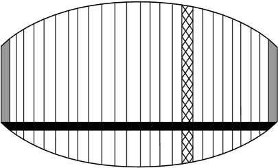
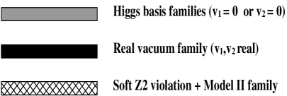
Figure 1: Schematic presentation of reparametrization equivalent space of Lagrangians. Different strips represent families with different explicit properties. A particular case when the soft $Z_{2}$ violating and Model II Lagrangians families coincide is shown.

All in principle observable quantities are IRpaT. That are, for example masses of observable Higgs bosons. Each of them is determined as eigenvalues of mass matrix (32) and (30). The coefficients of secular equation for diagonalization of this mass matrix (32) (among them – trace of this matrix and its determinant) can be constructed from these eigenvalues. Therefore, they are also IRpaT. The same is valid for the eigenvalues of Higgs-Higgs scattering matrices. The set of these IRpaT, classified in respect of isospin and hypercharge of Higgs-Higgs system, is presented in ref. unitCP1 .

The approach for construction of invariants of reparametrization transformations (IRpaT) is proposed in GH05 . The group–theoretical approach for construction of all independent invariants of this transformation is presented in ref. Iv05 .

$\bullet$ In the ${\varkappa}\neq 0$ case the transformation (5) induces in addition change of the kinetic term (4d):

$$T=z_{1}^{-1}(D_{\mu}\phi^{\prime}_{1})^{\dagger}(D^{\mu}\phi^{\prime}_{1})+z_{2}^{-1}(D_{\mu}\phi^{\prime}_{2})^{\dagger}(D^{\mu}\phi^{\prime}_{2})$$

$$+{\varkappa}^{\prime}(D_{\mu}\phi^{\prime}_{1})^{\dagger}(D^{\mu}\phi^{\prime}_{2})+{\varkappa}^{\prime*}(D_{\mu}\phi^{\prime}_{2})^{\dagger}(D^{\mu}\phi^{\prime}_{1})$$ (7)

with

$$\begin{array}[]{c}z_{1}^{-1}=1-2cs\thinspace{\rm Re\thinspace}(e^{-i\tau}{\varkappa}),\;\,z_{2}^{-1}=1+2cs\thinspace{\rm Re\thinspace}(e^{-i\tau}{\varkappa}),\\[5.69054pt] {\varkappa}^{\prime}=e^{-i\rho}(c^{2}{\varkappa}-s^{2}e^{2i\tau}{\varkappa}^{*}).\end{array}$$

So, in order to restore a canonical form of the kinetic term a field renormalization is needed in addition to the transformations (6). This case will be discussed in more detail elsewhere.

Remark on physical parameters.

Some parameters of theory which are treated often as physical (and in principle measurable) ones are in fact reparametrization dependent. The most important example provides a ratio of vacuum expectation values of scalar fields, $\tan\beta$ (19). For example, under the transformation (5) with $\rho=\xi$ (see eq. (19b)) and $\tau=0$, angle $\beta$ changes to $\beta+\theta$.

II.1.2 Rephasing invariance

It is useful to consider a particular case of the transformations (5) with $\theta=0$. It can be also treated as a global transformation of fields with independent phase rotations (rephasing transformation of the fields):

$$\begin{array}[]{c}\phi_{k}\to e^{-i\rho_{i}}\phi_{k},\quad(k=1,2),\\[5.69054pt] \rho_{1}=\rho_{0}-\dfrac{{\rho}}{{2}},\;\,\rho_{2}=\rho_{0}+\dfrac{{\rho}}{{2}},\;\,\rho=\rho_{2}-\rho_{1}.\end{array}$$ (8)

This transformation leads to a change of phase of some coefficients of Lagrangian (the rephasing transformation (RPhT)   of   the parameters):

$$\begin{array}[]{c}\lambda_{1-4}\to\lambda_{1-4},\;\,m_{11}^{2}\to m_{11}^{2},\;\,m_{22}^{2}\to m_{22}^{2},\\[8.53581pt] \lambda_{5}\to\lambda_{5}\,e^{-2i\rho},\;\;\lambda_{6,7}\to\lambda_{6,7}\,e^{-i\rho},\\[5.69054pt] m_{12}^{2}\to m_{12}^{2}e^{-i\rho},\,\;{\varkappa}\to{\varkappa}\,e^{-i\rho}.\end{array}$$ (9)

By construction, the Lagrangian of the form (4) with coefficients $\lambda_{i}$, $m_{ij}^{2}$ and that with coefficients given by eq. (9) describe the same physical reality. We call this property a rephasing invariance; it is similar to the definition given in Branco .

The transformations (9) represent the one–parametrical rephasing transformation group with parameter $\rho$. By construction, this group is a subgroup of the reparametrization transformation group.

The one–dimensional rephasing equivalent space, is a subspace of the entire 3-dimensional reparametrization equivalent space of Lagrangians. The rephasing equivalent space is given by the sets of parameters of Lagrangians at different $\rho$. One can say that the entire reparametrization equivalent space is sliced to the rephasing equivalent subspaces (represented by the vertical strips in FIG. 1).

Remarks

$\bullet$ The concept of the rephasing invariance is easily extended to the description of a whole system of scalars and fermions by adding to the transformation (9) transformations (45axb) for the Yukawa parameters.

The transformation for scalar fields (5) evidently induces changes into the set of Yukawa parameters. This may hide some properties of the Yukawa Lagrangian, which are explicit in a definite scalar basis (e.g. Model I or Model II, see sec. IV). The Kobyashi – Maskawa matrix represents the reparameterization transformation from the quark basis of QCD to the electroweak basis.

$\bullet$ We will see that CP symmetry is conserved in the Higgs sector if there exists a Lagrangian in the form (4 with all parameters real. Obviously, this violation does not appear if the Lagrangian with complex parameters can be transformed by means of some RPaT (6) to a form with all parameters real.

II.2 Lagrangian and $Z_{2}$ symmetry

The violation of the $Z_{2}$ symmetry (2) in the Lagrangian allows for the $\phi_{1}\leftrightarrow\phi_{2}$ transitions. The general Higgs Lagrangian ${\cal L}_{H}$ (4) violates $Z_{2}$ symmetry by terms of the operator dimension 2 (with $m_{12}^{2}$), what is called a soft violation of $Z_{2}$ symmetry, and of the operator dimension 4 (with $\lambda_{6,7}$ and ${\varkappa}$), called a hard violation of $Z_{2}$ symmetry.

An exact $Z_{2}$ symmetry.

This case is described by the Lagrangian ${\cal L}_{H}$ (4) with $\lambda_{6}=\lambda_{7}={\varkappa}=m_{12}^{2}=0$ and only one parameter $\lambda_{5}$ can be complex. The RPhT (9) with a suitable phase $\rho$ allows to get another form of Lagrangian with a real $\lambda_{5}$, within the rephasing invariant space.

A soft violation of $Z_{2}$ symmetry.

In  the case of soft violation of $Z_{2}$ symmetry one adds to the $Z_{2}$ symmetric Lagrangian the term $m_{12}^{2}(\phi_{1}^{\dagger}\phi_{2})+h.c.$, with a generally complex $m_{12}^{2}$ (and $\lambda_{5}$) parameter. This type of violation respects the $Z_{2}$ symmetry at small distances (much smaller than $1/M$) in all orders of perturbative series, i.e. the amplitudes for $\phi_{1}\leftrightarrow\phi_{2}$ transitions disappear at virtuality $k^{2}\sim M^{2}\to\infty$. That is the reason for the name – a ”soft” violation. The RPhT’s (9) applied to the Lagrangian with a softly violated $Z_{2}$ symmetry can not change its character; they generate a whole soft $Z_{2}$ violating Lagrangian family (the crossed ”vertical” strip in FIG. 1).

A hard violation of $Z_{2}$ symmetry.

In the general case the terms of the operator dimension 4, with generally complex parameters $\lambda_{6}$, $\lambda_{7}$ and ${\varkappa}$, are added to the Lagrangian with a softly violated $Z_{2}$ symmetry. This is called a hard violation of $Z_{2}$ symmetry. This case includes both the opportunity of a hidden soft $Z_{2}$ symmetry violation (obtained from an exact or softly violated $Z_{2}$ symmetry case by a general RPaT) and of the true hard violation of $Z_{2}$ symmetry, which cannot be transformed to the case of exact or softly violated $Z_{2}$ symmetry by any RPaT (6). In the latter case the $Z_{2}$ symmetry is broken at both large and small distances in any scalar basis.

II.3 The case of a hidden soft $Z_{2}$ violation

Let our physical system allows a description by the Lagrangian with exact or softly violated $Z_{2}$ symmetry ${\cal L}_{s}$. The general RPaT (6) converts this Lagrangian to a form ${\cal L}_{hs}$ with $\lambda_{6},\,\lambda_{7}\neq 0$ and ${\varkappa}=0$. We call ${\cal L}_{hs}$ - a Lagrangian with a hidden soft $Z_{2}$ violation.

To simplify discussion of such a case we first apply to ${\cal L}_{s}$ the RPhT (9) to eliminate the phase of $\lambda_{5}$. We obtain the Lagrangian ${\cal L}_{s}^{R}$ with real $\lambda_{5}$ (still $m_{12}^{2}$ can be complex leaving open an opportunity for CP violation). Then we apply to ${\cal L}_{s}^{R}$ a general RPaT (6) and obtain Lagrangian ${\cal L}_{hs}$ in the form (4), with generally complex $\lambda_{5}$ and nonzero $\lambda_{6,7}$ (but still ${\varkappa}=0$). We get from (6)

$$\begin{array}[]{c}\lambda^{\prime}_{1}=c^{2}\lambda_{1}+s^{2}\lambda_{2}-cs\Phi,\\[5.69054pt] \lambda^{\prime}_{2}=s^{2}\lambda_{1}+c^{2}\lambda_{2}-cs\Phi,\\[8.53581pt] \lambda^{\prime}_{3}=\lambda_{3}+cs\Phi,\quad\lambda^{\prime}_{4}=\lambda_{4}+cs\Phi,\\[8.53581pt] \lambda^{\prime}_{5}=e^{-2i\rho}\lambda_{5}+e^{2i\tau}[cs\Phi+2is^{2}\lambda_{5}\sin 2\tau],\\[5.69054pt] \lambda^{\prime}_{6}=\dfrac{{e^{i(\tau-\rho)}}}{{2}}\left[cs(\lambda_{1}-\lambda_{2})+A\right],\\[5.69054pt] \lambda^{\prime}_{7}=\dfrac{{e^{i(\tau-\rho)}}}{{2}}\left[cs(\lambda_{1}-\lambda_{2})-A\right],\\[5.69054pt] \mbox{ with }\\[5.69054pt] A=(c^{2}-s^{2})\Phi+2ics\lambda_{5}\sin 2\tau,\\[5.69054pt] \Phi=cs[\lambda_{1}+\lambda_{2}-2(\lambda_{3}+\lambda_{4}+\lambda_{5}\cos 2\tau)]\,.\end{array}$$ (10)

The eq-s (10) allow to find parameters of the Lagrangian ${\cal L}_{s}^{R}$ with the explicit soft violating $Z_{2}$ symmetry and real $\lambda_{5}$, once the parameters of ${\cal L}_{hs}$ are known. The procedure is as follows:
1) The value of $\tau-\rho$ is determined from the equation

$$\dfrac{{\lambda^{\prime}_{6}+\lambda^{\prime}_{7}}}{{\lambda^{{}^{\prime}*}_{6}+\lambda^{{}^{\prime}*}_{7}}}=e^{2i(\tau-\rho)}\,.$$ (11a)

2) After that one can determine angle $$\theta$$ via equation

$$\dfrac{{\lambda^{\prime}_{6}+\lambda^{\prime}_{7}}}{{\lambda^{\prime}_{1}-\lambda^{\prime}_{2}}}=e^{i(\tau-\rho)}\dfrac{{\tan 2\theta}}{{2}}\,.$$ (11b)

3) Next one can determine quantity $$\Phi 2cs\lambda_{5}\sin 2\tau$$ and via the real and imaginary parts of

$$e^{-i(\tau-\rho)}(\lambda^{\prime}_{6}\!-\!\lambda^{\prime}_{7})\!=\!(c^{2}-s^{2})\Phi\!+\!2ics\lambda_{5}\sin 2\tau.$$ (11c)

4) Then one can determine the angle $$\rho \lambda_{5}$$ and the parameter as the phase and the module of the quantity

$$e^{-i\rho}\lambda_{5}=\lambda^{\prime}_{5}-e^{2i(\tau-\rho)}[cs\Phi+2is^{2}\sin 2\tau\lambda_{5}]\,.$$ (11d)

5) Finally, all remaining quantities $$\lambda_{1-4}$$ can be determined easily from the first four equations (10).

Eqs. (11c) and (11d) represent two different ways of obtaining the parameter $\lambda_{5}$. Besides, quantity $\Phi$ can be obtained both via eq. (11c) and from basic definition $\Phi=\lambda_{1}+\lambda_{2}-2[\lambda_{3}+\lambda_{4}+\lambda_{5}\cos 2\tau]$. The existence of these two ways can be considered as two constraints on the Lagrangian. It shows explicitly that in this case the quartic sector is described by only 8 independent parameters ($\lambda_{1-5}$ and $\theta$, $\rho$, $\tau$) instead of 10 independent parameters of the general Lagrangian (4) ($\lambda_{1-4}$, $\thinspace{\rm Re\thinspace}\lambda_{5-7}$, $\thinspace{\rm Im\thinspace}\lambda_{5-7}$).

II.4 Some features of the true hard $Z_{2}$ violation

$\bullet$ The most general Higgs Lagrangian (4) cannot be transformed to the the form with $\lambda_{6}=\lambda_{7}=0$ by any RPaT. We denote this case as that with true hard $Z_{2}$ symmetry violation. Let us discuss briefly what should be done in this case with the mixed kinetic terms in Eq. (4d). First we observe that this mixed kinetic terms can be removed by the nonunitary transformation, e.g.

$$\!\!(\phi_{1}^{\,\prime},\!\phi_{2}^{\,\prime})\!\to\!\!\left(\!\dfrac{\sqrt{{\varkappa}^{*}}\phi_{1}\!+\!\sqrt{{\varkappa}}\phi_{2}}{2\sqrt{|{\varkappa}|(1\!+\!|{\varkappa}|)}}\!\pm\!\dfrac{\sqrt{{\varkappa}^{*}}\phi_{1}\!-\!\sqrt{{\varkappa}}\phi_{2}}{2\sqrt{|{\varkappa}|(1\!-\!|{\varkappa}|)}}\!\right)\!.\!\!$$ (12)

However, in presence of the $\lambda_{6}$ and $\lambda_{7}$ terms, the renormalization of quadratically divergent, non-diagonal two-point functions leads anyway to the mixed kinetic terms (e.g. from loops with $\lambda_{6}^{*}\lambda_{1,3-5}$ and $\lambda_{7}^{*}\lambda_{2-5}$). It means that ${\varkappa}$  becomes nonzero at the higher orders of perturbative theory, and vice versa a mixed kinetic term generates counter-terms with $\lambda_{6,7}$. Therefore all of these terms should be included in Lagrangian (4a) on the same footing, i.e. the treatment of the hard violation of $Z_{2}$ symmetry without ${\varkappa}$ terms is inconsistent (see also Ginzburg1977 ; Wein90 ). (The phenomenon is analogous to a need of a quartic coupling of the form $\lambda\phi^{4}$ in the renormalization of the $\bar{\psi}\gamma^{5}\psi\phi\;$ theory bogoliubov .) Note that the parameter ${\varkappa}$ is generally running like parameters $\lambda$’s. Therefore, the Lagrangian remains off–diagonal in fields $\phi_{1,2}$ even at very small distances, above the EWSB transition. Such theory seems to be unnatural.

$\bullet$ To find a signature of this case in the arbitrary form of Lagrangian it is useful to consider a polarization operator matrix for two fields: ${\cal P}=\begin{pmatrix}\Pi_{11}&\Pi_{12}\\ \Pi_{21}&\Pi_{22}\end{pmatrix}$. In the general case the ratio $\Pi_{12}/(\Pi_{11}-\Pi_{22})$ is a running quantity at large Higgs boson virtuality $k^{2}$ in contrast to the case of a hidden $Z_{2}$ symmetry, where this ratio is not running.

Indeed, let us consider the Lagrangian with soft violation of $Z_{2}$ symmetry, ${\cal L}_{s}$, like in sect II.3. The one–loop polarization operator matrix for two fields has a form ${\cal P}=\begin{pmatrix}\Pi_{1}^{s}&0\\ 0&\Pi_{2}^{s}\end{pmatrix}k^{2}+\mbox{\it finite terms},$ for $k^{2}\to\infty$. The elements $\Pi_{1}^{s}$ and $\Pi_{2}^{s}$ describe renormalization of fields $\phi_{1}$ and $\phi_{2}$, respectively. There is no mixed kinetic term, and the $\phi_{1}\leftrightarrow\phi_{2}$ transitions at small distances are absent.

Under RPaT, the ${\cal L}_{s}$ is converted to the Lagrangian ${\cal L}_{hs}$, with nonzero $\lambda_{6}$ and $\lambda_{7}$ terms (10), still with ${\varkappa}=0$. This Lagrangian leads to the polarization operator with nonzero mixed term:

$$\begin{array}[]{c}\dfrac{{{\cal P}^{\prime}}}{{k^{2}}}=\begin{pmatrix}\Pi_{1}^{s}\cos^{2}\theta+\Pi_{2}^{s}\sin^{2}\theta&\Pi_{12}\\ \Pi_{12}^{*}&\Pi_{2}^{s}\cos^{2}\theta+\Pi_{1}^{s}\sin^{2}\theta\end{pmatrix},\\[11.38109pt] \Pi_{12}=(\Pi_{1}^{s}-\Pi_{2}^{s})e^{-i\tau}\sin\theta\cos\theta.\end{array}$$

Naively, this form of the polarization operator suggests that one should introduce in the Lagrangian the mixed kinetic term describing transitions $\phi^{\prime}_{1}\leftrightarrow\phi^{\prime}_{2}$. However, the renormalization group analysis ensures that in this case the ratio $\Pi_{12}/(\Pi_{11}-\Pi_{22})$ at large $k^{2}$ is renormalization invariant quantity (in contrast to the mentioned above case of the true hard violation of $Z_{2}$ symmetry). In such case there exist some parameters $\rho,\,\theta,\,\tau$ which restore the incident form of ${\cal L}_{H}$ with soft $Z_{2}$ symmetry violation, i.e. without kinetic terms. In such scalar basis the transitions $\phi_{1}\leftrightarrow\phi_{2}$ are absent at small distances. Since the kinetic term of Lagrangian can be obtained from the initial $diag(1,\,1)$ form by the orthogonal transformation (5), one can conclude that the mentioned relations among parameters of new quartic terms prevent an appearance of the mixed kinetic term in the Higgs Lagrangian in any reparametrization equivalent Lagrangians. As it was mentioned above, this is in contrast to the general case with the true hard violation of $Z_{2}$ symmetry, where $\phi_{1}\leftrightarrow\phi_{2}$ transitions at different large $k^{2}$ cannot be ruled out simultaneously by any RPaT (6).

The another example is given by the EWSB procedure (sec. II.5) in the case of soft violation of $Z_{2}$ symmetry. It transforms the Lagrangian expressed in terms of fields $\phi_{1,2}$ to that written in terms of Higgs fields $h_{1-3}$ and $H^{\pm}$. In this form many quartic couplings appear but there are some relations among them, since all of them were obtained from the initial Lagrangian ${\cal L}_{s}$ with 6 parameters ($\lambda_{1-4}$, $\thinspace{\rm Re\thinspace}\lambda_{5}$, $\thinspace{\rm Im\thinspace}\lambda_{5}$) and the orthogonal transformation from the ($\phi_{1},\,\phi_{2}$) basis to ($H^{\pm},\,h_{1},\,h_{2},\,h_{3}$) basis with the additional 3 parameters. In this Lagrangian a mixed polarization operator may also appear, however no mixed kinetic term in contrast to the case of true hard violation of $Z_{2}$ symmetry. This is due the mentioned relations among parameters of new quartic terms which prevent appearance of the mixed kinetic term in the Higgs Lagrangian Pilaf97 . The detailed discussion of these problems will be done elsewhere.

Other aspects of the hard violation of $Z_{2}$ symmetry are related to the description of Yukawa sector. This will be discussed in sec. IV.

Remarks

$\bullet$ The diagonalization described by Eq. (12) is rather special and it changes even the definitions of $\lambda$’s, what would destroy relatively simple relations between the masses of the Higgs bosons discussed below.

$\bullet$ Although in this paper we present relations for the case of hard violation of $Z_{2}$ symmetry at ${\varkappa}=0$ one should keep in mind that loop corrections can change results significantly. Such treatment of the case with hard violation of $Z_{2}$ symmetry is as incomplete as in most of the papers considering this ”most general 2HDM potential”. A full treatment of this problem goes beyond the scope of the present paper.

II.5 Vacuum

The extremes of the potential define the vacuum expectation values (v.e.v.’s $\langle\phi_{1,2}\rangle$) of the fields $\phi_{1,2}$ via equations:

$$\dfrac{\partial V}{\partial\phi_{1}}\bigg{|}_{\genfrac{}{}{0.0pt}{}{\phi_{1}=\langle\phi_{1}\rangle,}{\phi_{2}=\langle\phi_{2}\rangle}}=0,\qquad\dfrac{\partial V}{\partial\phi_{2}}\bigg{|}_{\genfrac{}{}{0.0pt}{}{\phi_{1}=\langle\phi_{1}\rangle,}{\phi_{2}=\langle\phi_{2}\rangle}}=0.$$ (13)

This equation has trivial electroweak symmetry conserving solution $\langle\phi_{1}\rangle=0$, $\langle\phi_{2}\rangle=0$ and electroweak symmetry violating solutions, discussed below. With accuracy to the choice of $z$ axis in the weak isospin space, and using the overall phase freedom of the Lagrangian to choose one vacuum expectation value real, most general electroweak symmetry violating solution can be written in a form

$$\langle\phi_{1}\rangle=\dfrac{{1}}{{\sqrt{2}}}\left(\begin{array}[]{c}0\\ v_{1}\end{array}\right),\;\;\langle\phi_{2}\rangle=\dfrac{{1}}{{\sqrt{2}}}\left(\begin{array}[]{c}u\\[14.22636pt] v_{2}e^{i\xi}\end{array}\right).$$ (14)

It is useful to describe the discussed extremes with the aid of quantities

$$y_{1}\!=\!\langle\phi_{1}^{\dagger}\rangle\langle\phi_{1}\rangle,\;\,y_{2}\!=\!\langle\phi_{2}^{\dagger}\rangle\langle\phi_{2}\rangle,\;\,y_{3}\!=\!\langle\phi_{1}^{\dagger}\rangle\langle\phi_{2}\rangle,$$

$$y_{3}y_{3}^{*}-y_{1}y_{2}\,.$$ (15)

II.5.1 $u\neq 0$ solution, charged vacuum

For

$$y_{3}^{*}y_{3}-y_{1}y_{2}\neq 0\;\;\mbox{we have}\;\;u\neq 0\,.$$ (16)

In this case the v.e.v.’s are given by equations

$$\begin{array}[]{c}\lambda_{1}y_{1}\!+\!\lambda_{3}y_{2}\!+\!\lambda_{6}^{*}y_{3}^{*}+\lambda_{6}y_{3}=m_{11}^{2}/2,\\[5.69054pt] \lambda_{2}y_{2}\!+\!\lambda_{3}y_{1}\!+\!\lambda_{7}^{*}y_{3}^{*}+\lambda_{7}y_{3}=m_{22}^{2}/2,\\[5.69054pt] \lambda_{4}y_{3}^{*}\!+\!\lambda_{5}y_{3}\!+\!\lambda_{6}y_{1}+\lambda_{7}y_{2}=m_{12}^{2}/2.\end{array}$$ (17)

Depending on the parameters of potential, the extremum given by this solution of (13) describes either saddle point or a minimum of the potential, denoted as a charged vacuum, with a heavy photon and other nonphysical properties Diaz-Cruz:1992uw , chargebr .

II.5.2 $u=0$ solution, physical (neutral) vacuum

Another solution of extremum condition (13) is realized at

$$y_{3}^{*}y_{3}-y_{1}y_{2}=0,\,\,\mbox{ which\,\, gives }\,\,u=0.$$ (18)

The solution has a form

$$\langle\phi_{1}\rangle\!=\!\dfrac{1}{\sqrt{2}}\begin{pmatrix}0\\[2.84526pt] v_{1}\end{pmatrix}\,\text{ and }\,\langle\phi_{2}\rangle\!=\!\dfrac{1}{\sqrt{2}}\begin{pmatrix}0\\[2.84526pt] v_{2}e^{i\xi}\end{pmatrix}$$ (19a)

It satisfies a condition for $$U(1)$$ symmetry of electromagnetism.

This extremum realizes minimum of potential if its parameters are such that all eigenvalues of mass squared matrix in this extremum point are non-negative, sec. V.2. In the analysis we consider only this very case. (At this set of parameters the vacuum energy corresponding to the solution (17) is larger than that for the solution (19) Diaz-Cruz:1992uw , chargebr .)

The v.e.v’s $v_{1,2}$ (and therefore parameters of whole Lagrangian) obey SM constraint: $v_{1}^{2}+v_{2}^{2}=v^{2}$, with $v=(\sqrt{2}G_{\rm F})^{-1/2}=246$ GeV. The another parameterization of these v.e.v.’s is also used:

$$v_{1}=v\cos\beta,\quad v_{2}=v\sin\beta,\quad\beta\in\left(0,\,\dfrac{\pi}{2}\right).$$ (19b)

The rephasing of fields (8) shifts the phase difference $\xi$ as

$$\xi\to\xi-\rho\,.$$ (20)

Therefore, the phase difference $\xi$  between the v.e.v.’s has no physical sense (it was discussed e.g. in Branco ).

The arbitrariness described by (20) allows to simplify further calculations in a following way. Let us take some Lagrangian describing our model and calculate v.e.v.’s (19). Than, by making the RPhT with $\rho=\xi$, we get the Lagrangian in a real vacuum form (a real vacuum Lagrangian) (and the potential in a real vacuum form). By definition, the relative phase of v.e.v.’s derived from this Lagrangian equals to zero. In accordance with eq. (9) we get now

$$\begin{array}[]{c}\lambda_{1-4,rv}=\lambda_{1-4},\;\,\lambda_{5,rv}=\lambda_{5}e^{-2i\xi},\\[5.69054pt] \lambda_{6,rv}=\lambda_{6}e^{-i\xi},\;\,\lambda_{7,rv}=\lambda_{7}e^{-i\xi},\\[5.69054pt] {\varkappa}_{rv}={\varkappa}e^{-i\xi},\;\,m_{12,rv}^{2}=m_{12}^{2}e^{-i\xi},\end{array}$$ (21)

where we denote the particular values of parameters of such Lagrangian (potential) by subscript rv.

The following combinations of parameters and new quantities are useful:

$$\begin{array}[]{c}\lambda_{3,rv}+\lambda_{4,rv}+\thinspace{\rm Re\thinspace}\lambda_{5,rv}=\lambda_{345,rv},\\ \dfrac{v_{1}}{v_{2}}\lambda_{6,rv}\pm\dfrac{v_{2}}{v_{1}}\lambda_{7,rv}=\left\{\begin{array}[]{c}\lambda_{67,rv},\\ \tilde{\lambda}_{67,rv},\end{array}\right.\\[11.38109pt] m_{12,rv}^{2}=2v_{1}v_{2}(\nu+i\delta).\end{array}$$ (22)

For given $v_{1,2}$ the extremum condition (13) does not constrain $\thinspace{\rm Re\thinspace}m_{12,rv}^{2}$, while it does so for $\thinspace{\rm Im\thinspace}m_{12,rv}^{2}$, allowing to express it via $\thinspace{\rm Im\thinspace}(\lambda_{5-7,rv})$:

$$\delta=\underbrace{0}_{Z_{2}\;sym}+\underbrace{\dfrac{{1}}{{2}}\,\thinspace{\rm Im\thinspace}\lambda_{5,rv}}_{soft}+\underbrace{\dfrac{{1}}{{2}}\,\thinspace{\rm Im\thinspace}\lambda_{67,rv}}_{hard}\,.$$ (23)

Here (and in the subsequent equations) the first underbraced term correspond to the $Z_{2}$ symmetric case, the second and third terms are added to each other in the case of explicitly soft and hard violation of $Z_{2}$ symmetry, respectively. In particular, in the $Z_{2}$ symmetric case ${m}_{12,rv}^{2}=0$ and consequently $\thinspace{\rm Im\thinspace}\lambda_{5,rv}=0$.

Beginning from here all expressions will be presented for the potential in a real vacuum form, without writing explicitly the subscript rv. We will explicitly comment when other forms of Lagrangian will be discussed.

Remarks

The set of real vacuum Lagrangians forms a subspace in the entire reparametrization equivalent space – the real vacuum Lagrangian family. It is pictured in FIG. 1 by black horizontal line. In different points of this subspace the $\tan\beta$ values are different.

II.5.3 Our form of the potential

It is useful for the subsequent calculations to describe the potential in terms of $v_{1}$, $v_{2}$ and $\nu$ instead of three quadratic parameters $m_{11,22}^{2},m_{12}^{2}$ Pilaftsis:1999qt . The eq-s (13), (22) allow to obtain relations

$$\begin{array}[]{c}m_{11}^{2}\!=\!\underbrace{\lambda_{1}v^{2}_{1}\!+\!\lambda_{345}v_{2}^{2}}_{Z_{2}\;sym}\;\,\underbrace{\!-\!2\nu v^{2}_{2}}_{soft}\;\,+\underbrace{\dfrac{v_{2}}{v_{1}}\thinspace{\rm Re\thinspace}\left(3v_{1}^{2}\lambda_{6}\!+\!v_{2}^{2}\lambda_{7}\right)}_{hard},\\[19.91692pt] m_{22}^{2}\!=\!\underbrace{\lambda_{2}v^{2}_{2}\!+\!\lambda_{345}v_{1}^{2}}_{Z_{2}\;sym}\;\,\underbrace{\!-\!2\nu v^{2}_{1}}_{soft}+\underbrace{\dfrac{v_{1}}{v_{2}}\thinspace{\rm Re\thinspace}\left(v_{1}^{2}\lambda_{6}\!+\!3v_{2}^{2}\lambda_{7}\right)}_{hard}.\end{array}$$ (24)

From these relations we obtain another form of real vacuum potential, used in this paper:

$$\begin{array}[]{c}V\!=\!\dfrac{\lambda_{1}}{2}\left[(\phi_{1}^{\dagger}\phi_{1})\!-\!\dfrac{v_{1}^{2}}{2}\right]^{2}\!\!+\!\dfrac{\lambda_{2}}{2}\left[(\phi_{2}^{\dagger}\phi_{2})\!-\!\dfrac{v_{2}^{2}}{2}\right]^{2}\\[8.53581pt] +\lambda_{3}(\phi_{1}^{\dagger}\phi_{1})(\phi_{2}^{\dagger}\phi_{2})+\lambda_{4}(\phi_{1}^{\dagger}\phi_{2})(\phi_{2}^{\dagger}\phi_{1})\\[8.53581pt] +\dfrac{1}{2}\left[\lambda_{5}(\phi_{1}^{\dagger}\phi_{2})^{2}+{\rm h.c.}\right]\\[5.69054pt] +\left\{\left[\lambda_{6}(\phi_{1}^{\dagger}\phi_{1})+\lambda_{7}(\phi_{2}^{\dagger}\phi_{2})\right](\phi_{1}^{\dagger}\phi_{2})+{\rm h.c.}\right\}\\[5.69054pt] -\dfrac{1}{2}\bigl{(}\lambda_{345}+2\thinspace{\rm Re\thinspace}\lambda_{67}\bigr{)}[v_{2}^{2}(\phi_{1}^{\dagger}\phi_{1})+v_{1}^{2}(\phi_{2}^{\dagger}\phi_{2})]\\[5.69054pt] -\,\thinspace{\rm Re\thinspace}[\lambda_{6}(\phi_{1}^{\dagger}\phi_{1})+\lambda_{7}(\phi_{2}^{\dagger}\phi_{2})]v_{1}v_{2}\\[5.69054pt] +\nu(v_{2}\phi_{1}-v_{1}\phi_{2})^{\dagger}(v_{2}\phi_{1}-v_{1}\phi_{2})\\[5.69054pt] +2\delta\,\thinspace{\rm Im\thinspace}(\phi_{1}^{\dagger}\phi_{2})v_{1}v_{2}-\lambda_{1}\dfrac{{v_{1}^{4}}}{{8}}-\lambda_{2}\dfrac{{v_{2}^{4}}}{{8}}.\end{array}$$ (25)

In this form the quartic terms are as those in the initial potential (4) but with particular values of parameters $\lambda_{i}$ equal to $\lambda_{i,rv}$ (21). The mass term is determined via v.e.v.’s $v_{1}$, $v_{2}$ and the parameters $\lambda_{i}$ plus a single free dimensionless parameter $\nu$. The quantity $\delta\propto\thinspace{\rm Im\thinspace}\,m_{12}^{2}$ is given by eq. (23). (Sometimes instead of $\nu$ a dimensional parameter $\mu$, defined via $\mu^{2}=\nu v^{2}$, is used.)

In the above equation the soft $Z_{2}$ violating contribution is written as a sum of two terms, so that the variation of each of them don’t influence v.e.v.’s. The derivatives of first term ($\propto\nu$) over $\phi_{k}$ are equal to zero at the extremum point $\langle\phi_{k}\rangle=v_{k}/\sqrt{2}$. The second term ($\propto\delta$) is equal to zero for real $\phi_{1,2}$, independently on their absolute values. This decomposition is less transparent in Lagrangians with $\xi\neq 0$.

The vacuum energy density given by minimum (19) is equal to

$$\begin{array}[]{c}E_{vac}\equiv V\left(\langle\phi_{1}\rangle,\langle\phi_{2}\rangle\right)=-\dfrac{{\lambda_{1}v_{1}^{4}}}{{8}}-\dfrac{{\lambda_{2}v_{2}^{4}}}{{8}}\\ -\lambda_{345}\dfrac{{v_{1}^{2}v_{2}^{2}}}{{4}}-\thinspace{\rm Re\thinspace}(\lambda_{6}v_{1}^{2}+\lambda_{7}v_{2}^{2})\dfrac{{v_{1}v_{2}}}{{2}}\,.\end{array}$$ (26)

Remark

The transformation (5) with $\tau=0$, $\theta=-\beta$ or $\theta=\pi/2-\beta$ gives ($v_{1}=v$, $v_{2}=0$) or ($v_{1}=0$, $v_{2}=v$), respectively. The sets of the obtained Lagrangians form a Higgs basis Lagrangian families, they are pictured as grey vertical strips in the reparameterization equivalent Lagrangian space presented in FIG. 1. These cases cannot be described by our potential (25) since some of the coefficients (22), (23), used at the transformation to this form, are singular at $v_{2}\to 0$ or $v_{1}\to 0$. For both these cases $\sin 2\beta=0$. Therefore, our analysis based on the potential (25) is valid only for Lagrangians with

$$\sin 2\beta\neq 0\,$$ (27)

(domain of entire reparametrization equivalent space of FIG. 1 between two grey strips). Some results for the Higgs basis Lagrangian can be found in higgsbasis ; Branco ; Higgsrep .

III Physical Higgs sector

The fields $\phi_{1,2}$ change under the transformation (5). We introduce now the, in principle, observable Higgs fields and their couplings. These fields and couplings are evidently reparametrization independent. (The reparametrization dependent are parameters describing the transformation to this physical basis, see below.)

A standard decomposition of the fields $\phi_{1,2}$ in terms of physical fields is made via

$$\phi_{1}\!=\!\begin{pmatrix}\varphi_{1}^{+}\\ \dfrac{v_{1}+\eta_{1}+i\chi_{1}}{\sqrt{2}}\end{pmatrix},\;\,\phi_{2}=\begin{pmatrix}\varphi_{2}^{+}\\ \dfrac{v_{2}+\eta_{2}+i\chi_{2}}{\sqrt{2}}\end{pmatrix}.$$ (28)

At ${\varkappa}=0$ such decomposition leads to a diagonal form of kinetic terms for new fields $\varphi_{i}^{+},\,\chi_{i},\,\eta_{i}$, while the corresponding mass matrix is off-diagonal. The mass-squared matrix can be transformed to the block diagonal form by a separation of the massless Goldstone boson fields, $G^{0}=\cos\beta\,\chi_{1}+\sin\beta\,\chi_{2}$ and $G^{\pm}=\cos\beta\,\varphi_{1}^{\pm}+\sin\beta\,\varphi_{2}^{\pm}$, and the charged Higgs boson fields $H^{\pm}$:

$$H^{\pm}=-\sin\beta\,\varphi_{1}^{\pm}+\cos\beta\,\varphi_{2}^{\pm}\,,$$ (29)

with the mass squared equal to

$$M_{H^{\pm}}^{2}=\left[\nu-\dfrac{1}{2}(\lambda_{4}+\thinspace{\rm Re\thinspace}\lambda_{5}+\thinspace{\rm Re\thinspace}\lambda_{67})\right]v^{2}.$$ (30)

III.1 Neutral Higgs sector. General introduction

By definition $\eta_{1,2}$ are the standard $C$– and $P$– even (scalar) fields. The field

$$A=-\sin\beta\,\chi_{1}+\cos\beta\,\chi_{2}\,,$$ (31)

is $C$–odd (which in the interactions with fermions behaves as a $P$– odd particle, i.e. a pseudoscalar). In other words, the $\eta_{1,2}$ and $A$ are fields with opposite CP parities (see e.g. Hunter for details). (Note that sometimes the set $\eta_{1}$, $\eta_{2}$ and $A$ is called the weak basis Branco .)

The decomposition (28) results in the (symmetric) mass–squared matrix $\cal M$ in the $\eta_{1}$, $\eta_{2}$, $A$ basis

$${\cal M}=\begin{pmatrix}M_{11}&M_{12}&M_{13}\\ M_{12}&M_{22}&M_{23}\\ M_{13}&M_{23}&M_{33}\end{pmatrix},$$ (32a)

with

$$M_{11}=\left[c_{\beta}^{2}\,\lambda_{1}+s_{\beta}^{2}\,\nu+s_{\beta}^{2}\thinspace{\rm Re\thinspace}(\dfrac{\lambda_{67}}{2}+\tilde{\lambda}_{67})\right]v^{2},$$

$$M_{22}=\left[s_{\beta}^{2}\,\lambda_{2}+c_{\beta}^{2}\,\nu+c_{\beta}^{2}\thinspace{\rm Re\thinspace}(\dfrac{\lambda_{67}}{2}-\tilde{\lambda}_{67})\right]v^{2},$$

$$M_{33}=\left[\nu-\thinspace{\rm Re\thinspace}(\lambda_{5}-\dfrac{1}{2}\lambda_{67})\right]v^{2},$$ (32b)

$$M_{12}=-\left[\nu-\lambda_{345}-\dfrac{3}{2}\thinspace{\rm Re\thinspace}\lambda_{67}\right]c_{\beta}s_{\beta}v^{2},$$

$$M_{13}=-\left[\delta+\dfrac{{1}}{{2}}\thinspace{\rm Im\thinspace}\tilde{\lambda}_{67}\right]s_{\beta}v^{2},$$

$$M_{23}=-\left[\delta-\dfrac{{1}}{{2}}\thinspace{\rm Im\thinspace}\tilde{\lambda}_{67}\right]c_{\beta}v^{2},$$

where we use abbreviations $$c_{\beta}=\cos\beta s_{\beta}=\sin\beta M_{33}$$, . As we discuss below is equal to the mass squared of the CP–odd Higgs boson in the CP conserving case, namely

$$M_{A}^{2}=M_{33}=\left[\nu-\thinspace{\rm Re\thinspace}(\lambda_{5}-\dfrac{1}{2}\lambda_{67})\right]v^{2}.$$ (32c)

The masses squared $M_{i}^{2}$ of the physical neutral states $h_{1-3}$ are eigenvalues of the matrix $\cal M$. These states are obtained from fields $\eta_{1},\,\eta_{2},\,A$ by a unitary transformation $R$ which diagonalizes the matrix $\cal M$:

$$\begin{array}[]{c}\begin{pmatrix}h_{1}\\ h_{2}\\ h_{3}\end{pmatrix}=R\begin{pmatrix}\eta_{1}\\ \eta_{2}\\ A\end{pmatrix}\,,\\[17.07164pt] \mbox{ with }\;\;R{\cal M}R^{T}=diag(M_{1}^{2},\,M_{2}^{2},\,M_{3}^{2})\,.\end{array}$$ (33)

The diagonalizing matrix $R$ can be written as a product of three rotation matrices described by three Euler angles $\alpha_{i}\in(0,\pi)$ (we define $c_{i}=\cos\alpha_{i}$, $s_{i}=\sin\alpha_{i}$):

$$\begin{array}[]{c}R=R_{3}R_{2}R_{1},\quad R_{1}=\begin{pmatrix}c_{1}&s_{1}&0\\ -s_{1}&c_{1}&0\\ 0&0&1\end{pmatrix},\\[19.91692pt] R_{2}\!=\!\begin{pmatrix}c_{2}&0&s_{2}\\ 0&1&0\\ -s_{2}&0&c_{2}\end{pmatrix},\;R_{3}\!=\!\begin{pmatrix}1&0&0\\ 0&c_{3}&s_{3}\\ 0&-s_{3}&c_{3}\end{pmatrix},\end{array}$$ (34a)

$$\begin{array}[]{c}R=\begin{pmatrix}R_{11}&R_{12}&R_{13}\\ R_{21}&R_{22}&R_{23}\\ R_{31}&R_{32}&R_{33}\end{pmatrix}\equiv\\[19.91692pt] \begin{pmatrix}c_{1}\,c_{2}&c_{2}\,s_{1}&s_{2}\\ \!-\!c_{1}\,s_{2}\,s_{3}\!-\!c_{3}\,s_{1}&c_{1}\,c_{3}\!-\!s_{1}\,s_{2}\,s_{3}&c_{2}\,s_{3}\\ \!-\!c_{1}\,c_{3}\,s_{2}\!+\!s_{1}\,s_{3}&\!-\!c_{1}\,s_{3}\!-\!c_{3}\,s_{1}\,s_{2}&c_{2}\,c_{3}\end{pmatrix}\,.\end{array}$$ (34b)

We adopt the convention for masses that $M_{2}\geq M_{1}$, but shall not require any other ordering.

In general, the obtained Higgs eigenstates $h_{i}$ (33) have no definite CP parity since they are mixtures of fields $\eta_{1,2}$ and $A$ having the opposite CP parities. This provides a CP nonconservation within the Higgs sector. The interaction of these Higgs bosons with matter explicitly violates the CP–symmetry. Such mixing (and violation of CP) is absent if $M_{13}=M_{23}=0$.

Remarks

$\bullet$ Note that in the case where there is an exact $Z_{2}$ symmetry and $\lambda_{5}=0$ there appears an additional Peccei–Quinn symmetry. Then $A$ is a massless Goldsone-like boson, $M_{A}=0$. The spontaneous violation of this symmetry results in a light particle with mass, which is generated due to non-perturbative effects.

$\bullet$ For the basic Higgs Lagrangian (4) in the case of a soft violation of $Z_{2}$ symmetry and Model II or I for the Yukawa interaction (see below), the perturbative corrections give no counter terms violating the $Z_{2}$ symmetry in a hard way. Therefore, with a suitable renormalization procedure, the mixed kinetic terms don’t appear in the Lagrangian in $h_{1-3}$ basis (the rotation (33) keeps kinetic term diagonal in all orders). At the same time, the mass terms and mixing angles $\alpha_{i}$ change due to the renormalization. Some aspects of this procedure were discussed in Pilaf97 .

III.2 Diagonalization of the scalar CP-even sector

It is useful to start with the diagonalization of scalar $\langle 12\rangle$  sector of matrix $\cal M$ which is given by the rotation matrix $R_{1}$. It results in the neutral, CP-even Higgs fields which we denote as $h$ and $(-H)$, while the CP–odd field $A$ remains unmixed. (Sign minus at $H$ is needed in order to match a standard convention used for CP-conserving case, see e.g. Hunter .) We got

$$\begin{array}[]{c}\begin{pmatrix}h\\ -H\\ A\end{pmatrix}=R_{1}\begin{pmatrix}\eta_{1}\\ \eta_{2}\\ A\end{pmatrix}\;\mbox{ with }\\[17.07164pt] R_{1}{\cal M}R_{1}^{T}={\cal M}_{1}\equiv\begin{pmatrix}M_{h}^{2}&0&M_{13}^{\prime}\\ 0&M_{H}^{2}&M_{23}^{\prime}\\ M_{13}^{\prime}&M_{23}^{\prime}&M_{A}^{2}\end{pmatrix}.\end{array}$$ (35)

with $M_{13}^{\prime},M_{23}^{\prime}$ given in eq.  (40).

Let us stress that in the general CP nonconserving case the states $h$, $H$ and $A$ have no direct physical sense, they are only subsidiary concepts useful in the calculations and discussions. In the case of CP conservation (realized for $M_{13}^{\prime}=M_{23}^{\prime}=0$) the fields $h$, $H$ and $A$ represent physical Higgs bosons: $h_{1}=h$, $h_{2}=-H$, $h_{3}=A$. This is why we use instead of $\alpha_{1}$ the mixing angle $\alpha\in(-\pi/2,\,\pi/2)$,

$$\alpha=\alpha_{1}-\pi/2\,,$$ (36)

which is customary for the CP–conserving case. Using this angle we get

$$\begin{array}[]{c}H=\cos\alpha\,\eta_{1}+\sin\alpha\,\eta_{2},\\[2.84526pt] h=-\sin\alpha\,\eta_{1}+\cos\alpha\,\eta_{2}.\end{array}$$ (37)

The diagonalization of the respective $\langle 12\rangle$ corner of mass-squared matrix $\cal M$ (32) results in

$$\begin{array}[]{c}M_{h,H}^{2}=\dfrac{1}{2}\left(M_{11}+M_{22}\mp{\cal N}\right),\\[11.38109pt] {\cal N}=\sqrt{(M_{11}-M_{22})^{2}+4M_{12}^{2}}.\end{array}$$ (38)

The following expressions for angles are useful in some applications:

$$\begin{array}[]{c}\cos 2\alpha=\dfrac{M_{11}-M_{22}}{M_{H}^{2}-M_{h}^{2}},\\[8.53581pt] \sin 2\alpha=\dfrac{2M_{12}}{M_{H}^{2}-M_{h}^{2}}\,,\\[8.53581pt] \dfrac{\sin 2\alpha}{\sin 2\beta}=\dfrac{(\lambda_{345}-\nu+3/2\thinspace{\rm Re\thinspace}\lambda_{67})v^{2}}{M_{H}^{2}-M_{h}^{2}}.\end{array}$$ (39)

III.3 Complete diagonalization

The above diagonalization keeps, in general, two off-diagonal elements in matrix ${\cal{M}}_{1}$ (35):

$$\begin{array}[]{c}M_{13}^{\prime}=c_{1}M_{13}+s_{1}M_{23}=\\[5.69054pt] -\left[\delta\cos(\beta+\alpha)-\dfrac{{Im\tilde{\lambda}_{67}}}{{2}}\cos(\beta-\alpha)\right]v^{2},\\[5.69054pt] \quad M_{23}^{\prime}=-s_{1}M_{13}+c_{1}M_{23}=\\[5.69054pt] \left[\delta\sin(\beta+\alpha)+\dfrac{{Im\tilde{\lambda}_{67}}}{{2}}\sin(\beta-\alpha)\right]v^{2}.\end{array}$$ (40)

If at least one of these off diagonal terms differs from zero, the additional diagonalization is necessary, and the mass eigenstates, being admixtures of CP–even and CP–odd states, violate the CP symmetry. In this case we express the physical Higgs boson states $h_{1-3}$ via $h$, $H$, $A$:

$$\begin{pmatrix}h_{1}\\ h_{2}\\ h_{3}\end{pmatrix}=R_{3}R_{2}\begin{pmatrix}h\\ -H\\ A\end{pmatrix}\;\mbox{ with}$$ (41)

$$R\,{\cal M}\,R^{T}=R_{3}R_{2}{\cal M}_{1}R_{2}^{T}R_{3}^{T}=\begin{pmatrix}M_{1}^{2}&0&0\\ 0&M_{2}^{2}&0\\ 0&0&M_{3}^{2}\end{pmatrix}.$$

The squared masses $M_{i}^{2}$ in Eq.(41) are the eigenvalues of the mass-squared matrix $\cal M$ (32), i.e. they are roots of the corresponding cubic equation (see solution, e.g., in ref. Dubinin:2002nx ). Note, that the trace of mass-squared matrix does not changed under the unitary transformations. Therefore, we have mass sum rule

$$\begin{array}[]{c}M_{1}^{2}+M_{2}^{2}+M_{3}^{2}=M_{h}^{2}+M_{H}^{2}+M_{A}^{2}\\[2.84526pt] =M_{11}+M_{22}+M_{33}\,.\end{array}$$ (42)

The relation (41) allows to discuss the general CP violating case in terms customary for the CP conserving one, i.e. with parameters $M_{H},\,M_{h}$, $M_{A}$ and $\alpha$. The angles $\alpha_{2}$, $\alpha_{3}$ describe mixing of the CP–even states ($h$, $H$) with the CP–odd state $A$.

III.4 Condition for CP violation.

The eq. (35) shows explicitly that the CP does not violated if and only if simultaneously

$$M^{\prime}_{13}=0\,,\quad M^{\prime}_{23}=0\,.$$ (43)

If these conditions are fulfilled, one can express the ratio $\thinspace{\rm Im\thinspace}\tilde{\lambda}_{67}/\delta$ in terms of angles $\beta$ and $\alpha$ by two relations which contradict each other at $\sin 2\beta\neq 0$ (27). Therefore, the CP violation in Higgs sector is absent if and only if $\thinspace{\rm Im\thinspace}\tilde{\lambda}_{67}=0$ and $\delta\propto\thinspace{\rm Im\thinspace}(m_{12}^{2})=0$. From the (23) it follows that the CP violation is absent if all coefficients in potential of a real vacuum form are real. Simple but cumbersome calculation shows that similar conclusion is valid also for the potential in a Higgs basis form, i.e. for $\sin 2\beta=0$. In other words, CP symmetry in Higgs sector is not violated if among different reparametrization equivalent potentials a potential with all real $\lambda_{i}$, $m^{2}_{ij}$ parameters can be found.

Vice versa, the complexity of some parameters of the potential in a real vacuum form is a sufficient condition for CP violation in the Higgs sector. For an arbitrary form of Lagrangian (in entire reparametrization space) the necessary and sufficient condition for CP violation in the Higgs sector can be written as complexity of some of combinations (which are invariant under RPhT, see (9))

$$\lambda_{5}^{*}(m_{12}^{2})^{2}\,,\quad\lambda_{6}^{*}m_{12}^{2}\,,\quad\lambda_{7}^{*}m_{12}^{2}\,.$$ (44)

Each this quantity is not reparametrization invariant one but they are very simple. (The condition for the case of explicit soft $Z_{2}$ violated potential was obtained in Froggatt:1992wt ). More complex form of conditions for CP violation can be written via invariants of RPaT invappr , GH05 .

III.5 Various cases of CP violation

Here we present various cases of CP violation.

$\bullet\,\,\,$ If δ=0$and$ Im ~λ_67=0, CP symmetry is not violated. The $h$, $H$ and $A$ are physical Higgs bosons, with masses given by eqs. (38) and (32c), and $\alpha_{2}=\alpha_{3}=0$.

$\bullet$ If ε_13≡—M_13’/ (M_A^2-M_h^2)—≪1 the Higgs boson $h_{1}$ practically coincides with $h$ ($\alpha_{2}\approx 0$). The interaction of $h_{1}$ with other particles respects CP–symmetry (with an accuracy $\sim{\varepsilon}_{13}$). The diagonalization of the residual $\langle 23\rangle$ corner of mass-squared matrix (35) with the aid of rotation matrix $R_{3}$ (34a) gives states $h_{2}$ and $h_{3}$. They are superpositions of $H$ and $A$ states with potentially large mixing angle $\alpha_{3}$:

$$\tan 2\alpha_{3}\approx\dfrac{-2M^{\prime}_{23}}{M_{A}^{2}-M_{H}^{2}}\,,\;\;\alpha_{2}\approx 0.$$ (45a)

If $$M_{A}\approx M_{H} |M^{\prime}_{23}|/v^{2} h_{2} h_{3} |M_{2}^{2}-M_{3}^{2}| |M_{H}^{2}-M_{A}^{2}| M_{H}\approx 300 |M_{H}-M_{A}|\approx 5 M^{\prime}_{23}\approx 0.02\,v^{2} |M_{2}^{2}-M_{3}^{3}|\approx 25 \sin 2\alpha_{3}\approx 0.8$$, the CP violating mixing can be strong even at small but nonzero . The states and have no definite CP parity and the mass difference is larger than . For example, at GeV, GeV and we have GeV, .

At the growth of $M_{H}\approx M_{A}$ the proper widths of $H$ and $A$ become large so that the $H$ and $A$ peaks overlap strong. In such case the tree approximation may be too rough for a reliable calculation of masses $M_{i}$ and mixing angles. Therefore one should supplement the mass-squared matrix (32) by a (complex) matrix of Higgs polarization operators as it is customary in the description of low energy phenomena (see discussion in sec. VI.1).

$\bullet$ If ε_23 ≡—M_23’/(M_A^2-M_H^2)—≪1, the Higgs boson $h_{2}$ practically coincides with $-H$ ($\alpha_{3}\approx 0$). The interaction of matter with $h_{2}$ does not violate CP–symmetry. Similarly to the previous case, the diagonalization of the $\langle 13\rangle$ part of mass-squared matrix (35), with the aid of rotation matrix $R_{2}$ (34a), gives states $h_{1}$ and $h_{3}$. They are superpositions of $h$ and $A$ states with potentially large mixing angle $\alpha_{2}$:

$$\tan 2\alpha_{2}\approx\dfrac{-2M^{\prime}_{13}}{M_{A}^{2}-M_{h}^{2}}\,,\;\;\alpha_{3}\approx 0.$$ (45b)

Similarly to the previous case, if $M_{A}\approx M_{h}$, the CP violating mixing can be strong even at small $M^{\prime}_{13}/v^{2}$.

$\bullet$ Case of a weak CP violation combines both described above cases (45). If both $|M^{\prime}_{13}|\ll|M_{A}^{2}-M_{h}^{2}|$ and $|M^{\prime}_{23}|\ll|M_{A}^{2}-M_{H}^{2}|$ the CP–even states $h$, $H$ are weakly mixed with the CP–odd state $A$, and parameters $\alpha_{2}$ and $\alpha_{3}$ are simultaneously small:

$$\begin{array}[]{c}\tan\alpha_{2}\approx s_{2}\approx\dfrac{-M_{13}^{\prime}}{M_{A}^{2}-M_{h}^{2}}\approx\alpha_{2}\,,\\[8.53581pt] \tan\alpha_{3}\approx s_{3}\approx\dfrac{-M_{23}^{\prime}}{M_{A}^{2}-M_{H}^{2}}\approx\alpha_{3}\\[8.53581pt] (|\alpha_{2}|,|\alpha_{3}|\ll 1).\end{array}$$ (45ata)

To the second order in $s_{2}$ and $s_{3}$ the corresponding masses are

$$\begin{array}[]{c}M_{1}^{2}=M_{h}^{2}-s_{2}^{2}(M_{A}^{2}-M_{h}^{2}),\\[2.84526pt] M_{2}^{2}=M_{H}^{2}-s_{3}^{2}(M_{A}^{2}-M_{H}^{2}),\end{array}$$ (45atb)

with $M_{3}$ given by the sum rule (42) .

In the particular case of a soft violation of $Z_{2}$ symmetry we have

$$s_{2}\!\approx\!\delta\,\dfrac{\cos(\beta+\alpha)}{M_{A}^{2}\!-\!M_{h}^{2}}v^{2},\;s_{3}\!\approx\!-\delta\,\dfrac{\sin(\beta+\alpha)}{M_{A}^{2}\!-\!M_{H}^{2}}v^{2}.$$ (45atc)

$\bullet$ The case of intense coupling regime with $M_{A}\approx M_{h}\approx M_{H}$ intense may also give strong CP violating mixing even with small both $\delta$ and $\thinspace{\rm Im\thinspace}\tilde{\lambda}_{67}$.

Remark

Note that in MSSM, etc. CP symmetry can be violated by interaction of Higgs fields with different scalar squarks, etc. In this case the mixed polarization operators $\thinspace{\rm Im\thinspace}\Pi_{HA}$ and $\thinspace{\rm Im\thinspace}\Pi_{hA}$ appear leading to the CP violation in Higgs sector even for the CP conserving Higgs potential. This violation can be visible if $H$ and $A$ or (and) $h$ and $A$ are almost degenerate (see e.g. EllPilaf and references therein).

III.6 Couplings to gauge bosons

The gauge bosons $V$ ($W$ and $Z$) couple only to the CP–even fields $\eta_{1}$, $\eta_{2}$. For the physical Higgs bosons $h_{i}$ (33) one obtains simple expressions for their couplings, which in terms of the relative couplings (3) read

$$\begin{array}[]{c}\chi_{V}^{(i)}\!=\!\cos\beta\,R_{i1}\!+\!\sin\beta\,R_{i2},\;\,V=W\mbox{ or }Z.\end{array}$$ (45aua)

Note that due to unitarity of the transformation matrix $R$, the following sum rule takes place sumrule :

$$\sum\limits_{i=1}^{3}(\chi_{V}^{(i)})^{2}=1\,.$$ (45aub)

In particular, in the case of weak violation of the CP symmetry considered above, with $s_{2}$, $s_{3}$ given by eqs. (45ata), we obtain

$$\begin{array}[]{c}\chi_{V}^{(1)}=\sin(\beta-\alpha),\;\,\chi_{V}^{(2)}=-\cos(\beta-\alpha),\\ \chi_{V}^{(3)}=-s_{2}\sin(\beta-\alpha)+s_{3}\cos(\beta-\alpha).\end{array}$$ (45av)

III.7 Higgs self-couplings

The decomposition of the scalar fields $\phi_{1,2}$ in terms of physical fields $h_{i}$ allows to identify the trilinear and quartic couplings among them via parameters of Lagrangian and elements of mixing matrix (34). They were obtained in Choi:1999uk ; Carena:2002bb ; Akhmetzyanova:2004cy . For completeness, we present them for our specific form of Lagrangian (25) in the Appendix.

In the case of soft $Z_{2}$ symmetry violation in the CP conservation case these equations simplify and we present in the Appendix self–couplings in this particular case as well.

For this very case we present two useful forms for triliniear couplings. First, we express these couplings in terms of masses and mixing angles $\alpha$ and $\beta$. Second, for the case of Model II for Yukawa interaction (see below) we find expressions for these trilinear couplings in terms of masses and relative couplings to gauge bosons and quarks (and the parameter $\nu$).

IV Yukawa interactions

IV.1 General discussion

In the general case the Yukawa Lagrangian reads Branco

$$\begin{array}[]{c}-{\cal L}_{\rm Y}=\bar{Q}_{L}[(\Gamma_{1}\phi_{1}+\Gamma_{2}\phi_{2})d_{R}\\[5.69054pt] +(\Delta_{1}\tilde{\phi}_{1}+\Delta_{2}\tilde{\phi}_{2})u_{R}]+{\rm h.c.},\end{array}$$ (45aw)

with similar terms for the leptons. Here, $Q_{L}$ refers to the 3-family vector of the left-handed quark doublets, whereas $d_{R}$ and $u_{R}$ refer to the 3-family vectors of the the right-handed field singlets (with $q_{\rm L}=(1-\gamma_{5})q/2$ and $\tilde{\phi}_{a}=i\tau_{2}\phi_{a}^{\dagger{\rm T}}$). The Yukawa matrices $\Gamma$ and $\Delta$ are 3–dimensional matrices in the family space with generally complex elements (Yukawa parameters).

Obviously the transformation (5) induces changes in the elements of matrices $\Gamma_{i}$ and $\Delta_{i}$. In particular, the rephasing invariance is extended to the full Higgs + Yukawa Lagrangian space if one supplements the transformations (8) of fields $\phi_{1,2}$ by the following transformations of fermion fields

$$\begin{array}[]{c}Q_{Lk}\to Q_{Lk}e^{i\tau_{qk}},\\[5.69054pt] d_{Rk}\to d_{Rk}e^{i(\tau_{qk}+\tau_{dk})},\\[5.69054pt] u_{Rk}\to u_{Rk}e^{i(\tau_{qk}+\tau_{uk})}.\end{array}$$ (45axa)

The corresponding transformations of the parameters of Yukawa Lagrangian supplementing the transformations (9) are

$$\begin{array}[]{c}\Gamma_{1}\,\to\,\Gamma_{1}\begin{pmatrix}e^{i\tau_{d1}}\\ e^{i\tau_{d2}}\\ e^{i\tau_{d3}}\end{pmatrix}e^{-i\rho_{1}},\;\Delta_{1}\,\to\,\Delta_{1}\begin{pmatrix}e^{i\tau_{u1}}\\ e^{i\tau_{u2}}\\ e^{i\tau_{u3}}\end{pmatrix}e^{i\rho_{1}},\\[14.22636pt] \Gamma_{2}\,\to\,\Gamma_{2}\begin{pmatrix}e^{i\tau_{d1}}\\ e^{i\tau_{d2}}\\ e^{i\tau_{d3}}\end{pmatrix}e^{-i\rho_{2}},\;\Delta_{2}\,\to\,\Delta_{2}\begin{pmatrix}e^{i\tau_{u1}}\\ e^{i\tau_{u2}}\\ e^{i\tau_{u3}}\end{pmatrix}e^{i\rho_{2}}.\end{array}$$ (45axb)

An existence of the off-diagonal (in family index) terms in the Yukawa matrices results in the flavor-changing neutral-currents (FCNC). The rephasing invariance under the transformations (8), (45axb) allows to make real the diagonal elements of only one matrix $\Gamma$ and one matrix $\Delta$. Complex values of the other elements of matrices $\Gamma_{1,2}$ and $\Delta_{1,2}$ can result in the complex values of one–loop corrections to some $\lambda$’s and in consequence to the CP violation in the Higgs sector discussed above (even for real bare coefficients $m_{12}^{2}$ and $\lambda$’s). In the latter case, the corresponding CP violating terms should be included in the Higgs Lagrangian in order to have a standard multiplicative renormalizability.

Note, that in the case when simultaneously $\Gamma_{1}\neq 0$ and $\Gamma_{2}\neq 0$ or $\Delta_{1}\neq 0$ and $\Delta_{2}\neq 0$ (i.e. right-handed fermion of the type $d_{R}$ or $u_{R}$ interacts with both fields $\phi_{1}$ and $\phi_{2}$), the counter terms corresponding to the one-loop corrections to the Higgs Lagrangian contain operators of dimension 4, which violate $Z_{2}$ symmetry (2) in a hard way. They contribute to the renormalization of parameters ${\varkappa}$, $\lambda_{6}$ and $\lambda_{7}$ Ginzburg1977 , Froggatt:1992wt . Therefore, to have only the soft violation of $Z_{2}$ symmetry (to prevent $\phi_{1}\leftrightarrow\phi_{2}$ transitions at small distances), one demands that Glashow:1977nt ; Paschos:1976ay

$$\begin{array}[]{c}\mbox{\it each right-handed fermion couples to}\\ \mbox{\it only one scalar field, either $\phi_{1}$ or $\phi_{2}$.}\end{array}$$ (45ay)

The case $\Gamma_{2}=\Delta_{1}=0$ with diagonal $\Gamma_{1}$, $\Delta_{2}$ corresponds to the well known Model II, while $\Gamma_{2}=\Delta_{2}=0$ – to the Model I (see  e.g. Hunter ). For the Lagrangian having simultaneously Model II and soft $Z_{2}$ violated form these properties (i.e. soft $Z_{2}$ violation and (45ay)) are stable under the radiative corrections. Note that general RPaT makes these properties of Lagrangian hidden.

If for a given physical system both the Model II (or Model I) and the soft $Z_{2}$ violating Lagrangians exist but don’t coincide, the radiative corrections transform a Lagrangian to that with a true hard violation of $Z_{2}$ symmetry. In this case only a general model like Model III and with true hard violation of the $Z_{2}$ symmetry is renormalizable. We don’t study this case considering it as unnatural.

IV.2 Model II

We limit ourselves to the case when the physical reality allows for the description of Higgs–fermion interaction in a form, where the fundamental scalar field $\phi_{1}$ couples to $d$-type quarks and charged leptons $\ell$, while $\phi_{2}$ couples to $u$-type quarks (we take neutrinos to be massless) – the Model II Lagrangians, which are represented by a crossed vertical strip in FIG. 1.

Using matrices $\Gamma_{1}=diag(g_{d1},g_{d2},g_{d3})$ and $\Delta_{2}=diag(g_{u1},g_{u2},g_{u3})$, we get

$$\begin{array}[]{c}-{\cal L}_{Y}^{II}=\sum_{k=1,2,3}g_{dk}\bar{Q}_{Lk}\phi_{1}d_{Rk}\\[5.69054pt] +\sum_{k=1,2,3}g_{uk}\bar{Q}_{Lk}\tilde{\phi}_{2}u_{Rk}\\[5.69054pt] +\sum_{k=1,2,3}g_{\ell k}\bar{\ell}_{Lk}\phi_{1}\ell_{Rk}+{\rm h.c.}\end{array}$$ (45az)

Certainly, the general RPaT (6) transforms Yukawa Lagrangian to a form where this basic definition of Model II cannot be seen. That are hidden Model II forms of Lagrangian. In entire reparametrization equivalent space these Lagrangians form a family shown by a crossed vertical strip in FIG. 1 (in this figure we suggest that this family coincides with soft $Z_{2}$ symmetry violated family).

The suitable choice of phases in transformations (9) and (45axb) eliminates phase difference of vacuum expectation values and makes all Yukawa parameters real. It gives a Model II Lagrangian in a real vacuum form. We will use such Lagrangian below. It corresponds to the intersection of crossed and black strips in FIG. 1.

As it was written above, different forms of Lagrangian can have different values of $\tan\beta$. To underline that we use the mentioned Lagrangian, we will supply (only in this section) quantity $\beta$ in this case by a subscript II, $\beta\to\beta_{II}$.

Since v.e.v.’s of scalar fields are responsible for the fermion mass similarly as in the SM, the relative Yukawa couplings of the physical neutral Higgs bosons $h_{i}$ (3) are identical for all $u$–type and for all $d$–type quarks (and charged leptons). They can be expressed via elements of the rotation matrix $R$ (33):

$$\begin{array}[]{c}\chi_{u}^{(i)}=\dfrac{1}{\sin\beta_{II}}[R_{i2}-i\cos\beta_{II}\,R_{i3}],\\ \chi^{(i)}_{d}=\dfrac{1}{\cos\beta_{II}}[R_{i1}-i\sin\beta_{II}\,R_{i3}].\end{array}$$ (45ba)

(Note that e.g. the interaction $\bar{d}_{L}(g_{1}+ig_{2})d_{R}+h.c$ reads for the Dirac fermions as $\bar{d}(g_{1}-i\gamma_{5}g_{2})d$.)

In the particular case of weak CP violation (with small $s_{2}$, $s_{3}$ (45at)) these relative couplings, together with the corresponding ones to gauge bosons, are presented in Table 1.

For the interaction of the charged Higgs bosons e.g. with $t$-quark, the Lagrangian (45az) gives

$$\begin{array}[]{c}{\cal L}_{H^{-}tb}=\dfrac{{M_{t}}}{{v\sqrt{2}}}\cot\beta_{II}\;\bar{b}(1+\gamma^{5})H^{-}t\\[5.69054pt] +\dfrac{{M_{b}}}{{v\sqrt{2}}}\tan\beta_{II}\;\bar{b}(1-\gamma^{5})H^{-}t+h.c.\end{array}$$ (45bb)

Table 1: Basic relative couplings in the weak CP-conserving 2HDM (II). In the upper lines results for the case with no CP violation and in lower lines the corresponding corrections $\propto s_{2},\,s_{3}$ are presented.

	$\chi_{V}$	$\chi_{u}$	$\chi_{d}$
$h_{1}$	$\begin{array}[]{c}\sin(\beta_{II}-\alpha)\\ (+0)\end{array}$	$\begin{array}[]{c}\dfrac{{\cos\alpha}}{{\sin\beta_{II}}}\\ (-is_{2}\cot\beta_{II})\end{array}$	$\begin{array}[]{c}-\dfrac{{\sin\alpha}}{{\cos\beta_{II}}}\\ (-is_{2}\tan\beta_{II})\end{array}$
$h_{2}$	$\begin{array}[]{c}-\cos(\beta_{II}-\alpha)\\ (+0)\end{array}$	$\begin{array}[]{c}-\,\dfrac{{\sin\alpha}}{{\sin\beta_{II}}}\\ (-is_{3}\cot\beta_{II})\end{array}$	$\begin{array}[]{c}-\,\dfrac{{\cos\alpha}}{{\cos\beta_{II}}}\\ (-is_{3}\tan\beta_{II})\end{array}$
$h_{3}$	$\begin{array}[]{c}0\\ (-s_{2}\sin{(\beta_{II}-\alpha)}+s_{3}\cos{(\beta_{II}-\alpha)})\end{array}$	$\begin{array}[]{c}-i\cot\beta_{II}\\ (-s_{2}\dfrac{\sin\alpha}{\sin\beta_{II}}+s_{3}\dfrac{\cos\alpha}{\sin\beta_{II}})\end{array}$	$\begin{array}[]{c}-i\tan\beta_{II}\\ (+s_{2}\dfrac{\sin\alpha}{\cos\beta_{II}}+s_{3}\dfrac{\cos\alpha}{\cos\beta_{II}})\end{array}$

It is useful to express the relative coupling of the neutral scalar $h_{i}$ to the charged Higgs boson, in the cases of weak CP violating and soft $Z_{2}$-violation, via the relative couplings of this neutral Higgs boson to the gauge bosons and fermions:

$$\begin{array}[]{c}\chi_{H^{\pm}}^{(i)}=\left(1-\dfrac{{M_{i}^{2}}}{{2M_{H^{\pm}}^{2}}}\right)\chi_{V}^{(i)}\\[8.53581pt] +\dfrac{{M_{i}^{2}-\nu v^{2}}}{{2M_{H^{\pm}}^{2}}}\thinspace{\rm Re\thinspace}(\chi_{u}^{(i)}+\chi_{d}^{(i)}).\end{array}$$ (45bc)

IV.3 Set of useful relations in Model II

The unitarity of the mixing matrix $R$ allows to obtain a number of relations sumrule ; Ginzburg:2001ss ; Ginzburg:2002wt between the relative couplings of neutral Higgs particles to the gauge bosons (45aua) and fermions (45ba) (basic relative couplings). Since such couplings can be treated as measurable quantities, relations between them are especially useful in phenomenological analyses.

Let us remind that in these relations we use the quantity $\tan\beta_{II}$ which coincides with the ratio $v_{2}/v_{1}$ only for a Model II Lagrangian (and has no this simple sense for other forms of Lagrangian). It is described via the basic relative couplings for $h_{i}$ as

$$\!\!\tan^{2}\beta_{II}\!=\!{\dfrac{{(\chi_{V}^{(i)}\!-\!\chi_{d}^{(i)})^{*}}}{{\chi_{u}^{(i)}\!-\!\chi_{V}^{(i)}}}}\!=\!{\dfrac{{1\!-\!|\chi_{d}^{(i)}|^{2}}}{{|\chi_{u}^{(i)}|^{2}\!-\!1}}}=\!\dfrac{{\thinspace{\rm Im\thinspace}\chi_{d}^{(i)}}}{{\thinspace{\rm Im\thinspace}\chi_{u}^{(i)}}}\!.$$ (45bd)

Certainly, these expressions hold also for $h,H,A$, except the last one, which is absent for $h,H$.

1. The pattern relation among the basic relative couplings holds of each neutral Higgs particle $h_{i}$ (in particular also for $h,H,A$ in the case of CP conservation) Ginzburg:2001ss ; Ginzburg:2002wt :

$$\begin{array}[]{c}(\chi_{u}^{(i)}+\chi_{d}^{(i)})\chi_{V}^{(i)}=1+\chi_{u}^{(i)}\chi_{d}^{(i)}\,,\\[2.84526pt] \mbox{ or }\\[2.84526pt] (\chi_{u}^{(i)}-\chi_{V}^{(i)})(\chi_{V}^{(i)}-\chi_{d}^{(i)})=1-(\chi_{V}^{(i)})^{2}.\end{array}$$ (45be)

2. A vertical sum rule for each basic relative coupling $\chi_{j}$ for all three neutral Higgs bosons $h_{i}$ is given by Grzadkowski:1999ye :

$$\sum\limits_{i=1}^{3}(\chi_{j}^{(i)})^{2}=1\,\qquad(j=V,d,u)\,.$$ (45bf)

For couplings to the gauge bosons this sum rule, written also above in eq. (45aub), takes place independently on a particular form of the Yukawa interaction.

3. The relations (45ba) allow also to write for each neutral Higgs boson $h_{i}$ a horizontal sum rule Grzadkowski:1999ye :

$$|\chi_{u}^{(i)}|^{2}\sin^{2}\beta_{II}+|\chi_{d}^{(i)}|^{2}\cos^{2}\beta_{II}=1\,.$$ (45bg)

These sum rules guarantee that the cross section to produce each neutral Higgs boson $h_{i}$ (or $h,H,A$) of the 2HDM, in the processes involving Yukawa interaction, cannot be lower than that for the SM Higgs boson with the same mass Grzadkowski:1999ye .

4. Besides, the useful linear relation follows directly from Eqs. (45aua), (45ba):

$$\begin{array}[]{c}\chi_{V}^{(i)}=\cos^{2}\beta_{II}\,\chi_{d}^{(i)*}+\sin^{2}\beta_{II}\,\chi_{u}^{(i)}=\\[8.53581pt] =\cos^{2}\beta_{II}\,\chi_{d}^{(i)}+\sin^{2}\beta_{II}\,\chi_{u}^{(i)*}\Rightarrow\\[8.53581pt] \left\{\!\begin{array}[]{c}\chi_{V}^{(i)}\!=\!\thinspace{\rm Re\thinspace}\left(\cos^{2}\beta_{II}\chi_{d}^{(i)}\!+\!\sin^{2}\beta_{II}\chi_{u}^{(i)}\right),\\[5.69054pt] \thinspace{\rm Im\thinspace}\left(\cos^{2}\beta_{II}\chi_{d}^{(i)}-\sin^{2}\beta_{II}\chi_{u}^{(i)}\right)=0.\end{array}\right.\end{array}$$ (45bh)

5. The relation for CP violated parts of Yukawa couplings: is obtained by exclusion of $\beta_{II}$ from the equations (45bg), (45bh)

$$(1-|\chi_{d}^{(i)}|^{2})\,\thinspace{\rm Im\thinspace}\chi_{u}^{(i)}+(1-|\chi_{u}^{(i)}|^{2})\,\thinspace{\rm Im\thinspace}\chi_{d}^{(i)}=0\,.$$ (45bi)

IV.3.1 Some applications.

Let us remind that the relative couplings to quarks are generally complex in contrast to the couplings to gauge bosons. For $h_{i}$ (or $h,H,A$) we found the following results.

• From (45bg) we get

  $$\begin{array}[]{c}|\chi^{(i)}_{u}|\gg 1\;\Rightarrow\;\tan\beta_{II}\ll 1\,;\\ |\chi^{(i)}_{d}|\gg 1\;\Rightarrow\;\tan\beta_{II}\gg 1\,.\end{array}$$ (45bj)

It is instructive to consider now consequences of the relations (45be)–(45bf) for the case when some basic relative couplings of a Higgs boson are close to $\pm 1$.

• In virtue of (45bg) we have for moderate $\tan\beta$

  $$|\chi^{(i)}_{u}|\approx 1\;\Rightarrow\;|\chi^{(i)}_{d}|\approx 1.$$ (45bk)

Note, that if $\tan\beta$ is extremely large or extremely small, the horizontal sum rule allows $|\chi^{(i)}_{d}|$ to differ strong from 1 or $|\chi^{(i)}_{u}|$ to differ strong from 1, respectively (in agreement with  (45bj)).

Taking for definitness the case of $\chi_{j}^{(2)}\approx\pm 1$, we get:

• From (45bf),

  $$\begin{array}[]{c}\chi^{(2)}_{u}\approx\pm 1\;\Rightarrow\;\chi^{(1)}_{u}\approx\pm i\chi^{(3)}_{u}\,,\\ \chi^{(2)}_{d}\approx\pm 1\;\Rightarrow\;\chi^{(1)}_{d}\approx\pm i\chi^{(3)}_{d}\,.\end{array}$$ (45bl)

• For $\chi_{V}^{(2)}\sim\pm 1$

  $$\begin{array}[]{c}\mbox{\it if}\qquad\chi_{V}^{(2)}\approx\pm 1\\[5.69054pt] \Rightarrow\left\{\begin{array}[]{cl}(a)&\chi_{u}^{(2)}\approx\chi_{V}^{(2)}\;\;or\;\;\chi_{d}^{(2)}\approx\chi_{V}^{(2)}\,,\\[5.69054pt] (b)&\chi_{u}^{(2)}\approx\chi_{d}^{(2)}\approx\chi_{V}^{(2)}\,,\\[5.69054pt] (c)&\chi_{V}^{(1)}\approx\chi_{V}^{(3)}\approx 0\,,\\[5.69054pt] (d)&\chi_{u}^{(1)}\,\chi_{d}^{(1)}\approx\chi_{u}^{(3)}\,\chi_{d}^{(3)}\approx-1\,.\end{array}\right.\end{array}$$ (45bm)

The property (a) obtained from (4.8b), means that the coupling of $h_{2}$ to at least one fermion type ($u$ or $d$) is close to the $\chi_{V}^{(2)}$. The property (b) follows from property (a) and (45bh), at moderate $\tan\beta$. The fact that the couplings of Higgs bosons to gauge bosons are real leads, with the aid of (45bf), to the property (c). Taking into account property (c) and the pattern relation (4.8a)   we obtain property (d): the product of Yukawa couplings for other Higgs bosons (not $h_{2}$) is close to the corresponding product for pseudoscalar $A$ in the CP conserving case.

Certainly, results analogous to (45bl), (45bm) hold in the cases when $\chi_{j}^{(1)}\approx\pm 1$ or $\chi_{j}^{(3)}\approx\pm 1$.

IV.4 Comments on radiative corrections

All results described so far were obtained in the tree approximation. Let us discuss briefly the stability of relations (45be)–(45bi) among in principle measurable parameters of the model in respect to the radiative corrections (RC) (treated mainly as the one–loop effects).

Certainly, the observable quantities should be obtained from the Lagrangian (and potential) with RC. Then one can treat the presented relations (45be)–(45bi) as obtained from the renormalized parameters (the elements of mass-squared matrix $\cal M$, the v.e.v.’s ratio $\tan\beta$ (19b) and the corresponding Euler angles $\alpha_{i}$ of Eq. (34)).

The approach which we adopt in our analysis is to deal with the relative couplings (3) – the ratios of the couplings of each neutral Higgs boson $h_{i}$ to the gauge bosons $W$ or $Z$ and to quarks or leptons ($j=W,Z,u,d,\ell...$), to the corresponding SM couplings. We assume that for each such relative coupling the RC are included in both: the couplings of the 2HDM (in the numerator) and those of SM (in the denominator). The largest RC to the Yukawa $\phi\bar{q}q$ couplings are the one–loop QCD corrections due to the gluon exchange. They are identical in the SM and in the 2HDM. If they are relatively small, they cancel in both ratios $\chi_{u}$ and $\chi_{d}$. The same is valid for purely QED RC to all basic couplings as well as for electroweak corrections including virtual $Z$ or $W$ contributions.

The situation is different for the electroweak corrections containing Higgs bosons in the loops. They are different in the SM and 2HDM, moreover their values depend on the parameters of 2HDM. These type of RC may modify slightly some relations presented in sec. IV. However, it is naturally to expect that these RC are small (below 1 %) except for some small corners of parameter space.

A delicate problem appears in a description of RC for the physical states after EWSB. The physical Higgs states become unstable and they have no asymptotic states. Therefore, the scattering matrix, written in terms of these fields, becomes non-hermitian. In particular, the mass matrix for Higgs bosons, obtained from (32) with RC, become non-hermitian. Full treatment of this problem demands a subtle theoretical analysis. In practice, we limit ourselves to some reasonable approximations. The effects of instability can be neglected when these Higgs bosons are almost stable (their widths are much smaller than the masses and mass splittings). These effects should be taken into account in the case of the approximate mass degeneracy, i.e. when some of masses $M_{i}$ are very close to each other. In such case a good description of the masses and couplings is given by an approximation in which a (complex) matrix of polarization operators is added to the mass matrix (32).

V Constraints for Higgs Lagrangian

The parameters of Higgs potential are constrained by three types of conditions:

• positivity (vacuum stability) constraints

• minimum constraints

• tree-level unitarity and perturbativity constraints,

which we will discuss below. The positivity and unitarity constraints were discussed in literature till now only for the case of a soft $Z_{2}$ violation, and the unitarity constraints only in the CP conserving case. In the same case of soft $Z_{2}$ violation the latter constraints were extended to the CP non-conserving case in unitCP . Here we present some new results for the case of hard $Z_{2}$ symmetry violation (see unitCP1 ).

V.1 Positivity (vacuum stability) constraints

To have a stable vacuum, the potential must be positive at large quasi–classical values of fields $|\phi_{k}|$ (positivity constraints) for an arbitrary direction in the $(\phi_{1},\phi_{2})$ plane. These constraints were obtained for the case of soft $Z_{2}$ violation (see e.g. dema ; unitCP ; Kastening:1992by ; Gunion:2002zf ), they are

$$\begin{array}[]{c}\lambda_{1}>0\,,\quad\lambda_{2}>0,\;\,\lambda_{3}+\sqrt{\lambda_{1}\lambda_{2}}>0,\\ \lambda_{3}+\lambda_{4}-|\lambda_{5}|+\sqrt{\lambda_{1}\lambda_{2}}>0.\end{array}$$ (45bn)

To obtain these constraints it is enough to consider only quartic terms of the potential. Let $(\phi_{1}^{\dagger}\phi_{1})=x_{1}\geq 0$, $(\phi_{2}^{\dagger}\phi_{2})=x_{2}\geq 0$. Than $(\phi_{1}^{\dagger}\phi_{2})=\sqrt{x_{1}x_{2}}\,ce^{i\alpha}$ with $|c|\leq 1$ (due to Schwartz theorem). The quadratic form $V(x_{1},\,x_{2})$ should be positive at large $x_{i}$ at different $c$ and $\phi$. At $x_{2}=0$ or $x_{1}$ we obtain two first conditions. At $c=0$ the third inequality is derived. At $c=\pm 1$ with variation of $\alpha$ in respect to the phase of $\lambda_{5}$ we obtain the latter constraint.

V.2 Minimum constraints

The condition for vacuum (13) describes the extremum of potential but not obligatory the minimum. The minimum constraints are the conditions ensuring that above extremum is a minimum for all directions in $(\phi_{1},\phi_{2})$ space, except of the Goldstone modes (the physical fields provide the basis in the coset). This condition is realized if the mass-matrix squared for the physical fields is positively defined, which means that its eigenvalues, i.e. the physical mass squared, are positive: $M_{h_{1-3}}^{2},\;M_{H^{\pm}}^{2}>0$. In some applications the necessary conditions for that: positivity of all diagonal elements, principal minors and the determinant of mass-squared matrix in different forms (32) or (41), are useful (see discussion in sec. II.5).

V.3 Unitarity and perturbativity constraints

The quartic terms of Higgs potential ($\lambda_{i}$) are transformed to the quartic self–couplings of the physical Higgs bosons. They lead, in the tree approximation, to the s–wave Higgs-Higgs and $W_{L}W_{L}$ and $W_{L}H$, etc. scattering amplitudes for different elastic channels. These amplitudes should not overcome unitary limit for this partial wave – that is the tree-level unitarity constraint.

The unitarity constraint was obtained first Glashow:1977nt in the frame of minimal SM, with one Higgs doublet and Higgs potential $V=(\lambda/2)(\phi^{\dagger}\phi-v^{2}/2)^{2}$ as the condition $3\lambda\leq 8\pi$. In this model the Higgs-boson mass $M_{H}=v\sqrt{\lambda}$ and its width $\Gamma_{H}$, given mainly by a decay of Higgs boson to the longitudinal components of gauge bosons $W_{L}$, $Z_{L}$ (originated from the Goldstone components $G^{\pm}$), grow with $M_{H}$ as $M_{H}^{3}$. Therefore, the unitarity limit corresponds simultaneously to the case where $\Gamma_{H}\approx M_{H}$, so that the physical Higgs boson disappears. On the other hand it is well known that for $\lambda\gtrsim 8\pi$ at $\sqrt{s}>v\sqrt{\lambda}\gtrsim v\sqrt{8\pi}\approx 1.2$ TeV the Higgs boson self–interaction become strong, it is realized as a strong interaction of $W_{L}$ and $Z_{L}$ (appeared as a Goldstone modes of a Higgs doublet at EWSB). Therefore, the unitarity limit is a boundary (in $\lambda$’s space) between two different physical regimes. Below the unitarity limit we have more or less narrow Higgs boson with well known properties (and no strong interaction effects in the Higgs sector). Above the unitarity limit the Higgs boson disappears as a particle, discussion in terms of the observable Higgs particle becomes senseless, and the Higgs sector becomes strongly interacting.

Akeroyd et al. Akeroyd:2000wc have derived the unitarity constraints for the 2HDM without a hard violation of $Z_{2}$ symmetry for the CP conserving case, i.e. for real $\lambda_{1-5}$. In the general CP nonconserving case with soft violation of $Z_{2}$ symmetry the parameter $\lambda_{5}$ is complex. The application of the RPhT (9) allows to eliminate phase of $\lambda_{5}$, coming to the rephasing equivalent Lagrangian with real $\lambda_{5}^{s}\equiv|\lambda_{5}|$ ($m_{12}^{2}$ remains complex). Use of this Lagrangian allows to extend the results presented in Akeroyd:2000wc for unitary constraints to the CP nonconserving case unitCP .

In the considered cases the $Z_{2}$ symmetry is not violated by the quartic terms of potential. Unitarity constraints are written in ref. unitCP as the bounds for the eigenvalues $\Lambda^{Z_{2}parity}_{Y\sigma}$ of the high energy Higgs–Higgs scattering matrix for the different quantum numbers of an initial state: total hypercharge $Y$, weak isospin $\sigma$ and $Z_{2}$ parity. These bounds given separately for the $Z_{2}$-even ($\phi_{1}\phi_{1}$ and $\phi_{2}\phi_{2}$) and $Z_{2}$-odd ($\phi_{1}\phi_{2}$) initial states are as follows:

$$|\Lambda_{Y\sigma\pm}^{Z_{2}}|<8\pi\;\qquad\mbox{\it with }$$

$$\Lambda_{21\pm}^{even}=\dfrac{{1}}{{2}}\left(\lambda_{1}+\lambda_{2}\pm\sqrt{(\lambda_{1}-\lambda_{2})^{2}+4|\lambda_{5}|^{2}\,}\;\right),$$

$$\Lambda_{21}^{odd}=\lambda_{3}+\lambda_{4}\,,\quad\Lambda_{20}^{odd}=\lambda_{3}-\lambda_{4}\,,$$

$$\Lambda_{01\pm}^{even}=\dfrac{{1}}{{2}}\left(\lambda_{1}+\lambda_{2}\pm\sqrt{(\lambda_{1}-\lambda_{2})^{2}+4\lambda_{4}^{2}\,}\right),$$

$$\Lambda_{01\pm}^{odd}=\lambda_{3}\pm|\lambda_{5}|\,,$$ (45bo)

$$\Lambda_{00\pm}^{even}=\dfrac{{3(\lambda_{1}+\lambda_{2})\pm\sqrt{9(\lambda_{1}-\lambda_{2})^{2}+4(2\lambda_{3}+\lambda_{4})^{2}\,}}}{{2}},$$

$$\Lambda_{00\pm}^{odd}=\lambda_{3}+2\lambda_{4}\pm 3|\lambda_{5}|\,.$$

For real $\lambda_{5}$ these conditions coincide with those from Akeroyd:2000wc , obtained however without the above mentioned identification of various contributions.

At small $\nu$ these constraints result in moderately large upper bound of $600\div 700$ GeV for $M_{H}$, $M_{A}$, $M_{H^{\pm}}$ (see examples in Table 2 of sec. VI.2), see also e.g. Akeroyd:2000wc for the CP conserving case. At large $\nu$, all Higgs bosons except $h_{1}$ become heavy without violating of the unitary constraints (45bo).

The correspondence between a violation of the tree-level unitarity limit and a lack of realization of the Higgs field as a resonance (a particle), as in the minimal SM, takes place in the 2HDM only in the case when all constraints (45bo) are violated simultaneously. In the case when only some of these constraints are violated the physical picture become more complex. One can imagine, for example, a situation when some of the Higgs bosons are ”normal” scalars, i.e. their properties can be estimated perturbatively, while the others interact strongly at sufficiently high energy. In such case, the unitarity constraints work differently for different physical channels, in particular, for different Higgs bosons.

The perturbativity condition (constraint) for a validity of a tree approximation in the description of some particular phenomena (e.g. interactions of the lightest Higgs boson $h_{1}$) may be less restrictive than the presented above general unitarity constraints. The explicit form of the perturbativity constraint should be found, however this is a subject for a separate consideration. In particular, the effective parameters of perturbation theory for the Yukawa interaction is $g^{2}/(4\pi)^{2}$. Therefore, one of the necessary conditions for the smallness of radiative corrections is $|g|\ll 4\pi$.

V.4 The case of hard $Z_{2}$ violation

The analysis of the case with hard $Z_{2}$ violation (i.e. the potential with $\lambda_{6,7}$ terms) is more complicated. One can say definitely that the positivity constraints (45bn) are valid for some particular directions of a growth of the quasi-classic fields $\phi_{1,2}$. Similarly, unitarity constraints (45bo) hold for such transition amplitudes which don’t violate the $Z_{2}$ symmetry.

For the hard violation of $Z_{2}$ symmetry one should consider new directions in the $(\phi_{1},\phi_{2})$ space which appear due to $\lambda_{6}$, $\lambda_{7}$ terms and the processes like $\phi_{1}\phi_{1}\to\phi_{1}\phi_{2}$, which violate the $Z_{2}$ symmetry. Therefore the new positivity and unitarity constraints should include parameters $\lambda_{6}$, $\lambda_{7}$. In any case conditions (45bo) are necessary for unitarity unitCP1 .

VI Heavy Higgs bosons in 2HDM

Many analyses of 2HDM assume a SM–like physical picture: the lightest Higgs boson $h_{1}$ is similar to the Higgs boson of the SM while other Higgs bosons escape observation being too heavy. Besides, many authors assume in addition that masses of other Higgs bosons $M$ are close to the scale of new physics, $M\sim\Lambda$, and that the theory should possess an explicit decoupling property, i.e. the correct description of the observable phenomena must be valid for the (unphysical) limit $M\to\infty$ Kanemura:1996eq ; Ciafaloni:1996ur ; Malinsky:2002mq ; Kanemura:2002cc ; Gunion:2002zf . However, the 2HDM allows also for another realization of the mentioned SM–like physical picture.

Looking on formulae from sec. III we see that the large masses of Higgs particles may arise from large parameters $\nu$ or $\lambda^{\prime}s$, or both. Obviously, large values of $\lambda^{\prime}s$ may be in conflict with unitarity constraints, which is not the case for large $\nu$. Below we discuss these two very distinct sources of large masses, and their different phenomenological consequences.

VI.1 Decoupling of heavy Higgs bosons

In 2HDM the decoupling case corresponds to

$$\nu\gg|\lambda_{i}|\,.$$ (45bp)

That means that it can not be realized for the exact $Z_{2}$ symmetry. In the decoupling case equations for masses and mixing angles $\alpha_{i}$ (39) simplify. First we find, with accuracy up to the $\lambda/\nu$ terms, masses of the subsidiary Higgs states obtained at the first stage of diagonalization (35-40). From eqs. (38) we derive

$$\dfrac{{M_{h}^{2}}}{{v^{2}}}=\underbrace{c_{\beta}^{4}\lambda_{1}+s_{\beta}^{4}\lambda_{2}+2s_{\beta}^{2}c_{\beta}^{2}\lambda_{345}}_{soft}+\underbrace{4s_{\beta}^{2}c_{\beta}^{2}\thinspace{\rm Re\thinspace}\lambda_{67}}_{hard},$$

$$\dfrac{{M_{H}^{2}}}{{v^{2}}}=\underbrace{\nu+s_{\beta}^{2}c_{\beta}^{2}(\lambda_{1}+\lambda_{2}-2\lambda_{345})}_{soft}$$ (45bq)

$$-\underbrace{[(c_{\beta}^{2}-s_{\beta}^{2})\thinspace{\rm Re\thinspace}\tilde{\lambda}_{67}+(4s_{\beta}^{2}c_{\beta}^{2}-1/2)\thinspace{\rm Re\thinspace}\lambda_{67}]}_{hard}.$$

In the proper decoupling limit $\nu\to\infty$ we have $\beta-\alpha\to\pi/2$. It is useful to characterize a deviation from this limiting value by a parameter $\Delta_{\beta\alpha}=\pi/2-(\beta-\alpha)$. Using $s_{2\beta}=\sin 2\beta$, $c_{2\beta}=\cos 2\beta,$ we get from the second line of eq. (39):

$$\begin{array}[]{c}\Delta_{\beta\alpha}=-\dfrac{{L_{a}s_{2\beta}}}{{2\nu}}\,,\\ L_{a}=\underbrace{s_{\beta}^{2}\lambda_{2}-c_{\beta}^{2}\lambda_{1}+c_{2\beta}\lambda_{345}}_{soft}\\ +\underbrace{\thinspace{\rm Re\thinspace}(2c_{2\beta}\lambda_{67}-\tilde{\lambda}_{67})}_{hard}.\end{array}$$ (45br)

The subsequent complete diagonalization, described in sec. III.3, is simplified by condition (45bp). We get the following results.

VI.1.1 The lightest Higgs boson $h_{1}$.

The eq-s (40), (23) show that under the condition (45bp) the element $M^{\prime}_{13}$ of the matrix (35), responsible for the mixing of scalar $h$ with $A$, is small as compared to the mass difference $M_{A}^{2}-M_{h}^{2}\approx\nu v^{2}$. Therefore, the state $h_{1}$ is very close to $h$. The mixing angle $\alpha_{2}$, describing the CP–odd admixture in this state, is given by $s_{2}\sim|\lambda|/\nu(\ll 1)$ (45ata). The shift of the mass of $h_{1}$ from the $M_{h}$ value (45bq) is given by Eq. (45atc), i.e. $M_{1}^{2}-M_{h}^{2}\sim|\lambda|/\nu$, and can be neglected.

Since for $\nu\to\infty$ the $\Delta_{\beta\alpha}\to 0$ the scalar $h_{1}$ couples to the gauge bosons and to the quarks and leptons in the Model II as in the SM (with accuracy $|\lambda|/\nu$) even for the general CP non-conserving case. Besides, $h_{1}$ practically decouple from $H^{\pm}$, since the quantity $\chi^{(1)}_{H^{\pm}}\sim{\cal O}(|\lambda|/\nu)$ (45bc).

VI.1.2 Higgs bosons $h_{2},h_{3}$ and $H^{\pm}$.

The eqs.  (30), (32c), (45bq) show that

$$M_{H^{\pm}}^{2}\approx M_{A}^{2}\approx M_{H}^{2}=v^{2}{\nu}\left[1+{\cal O}\left(\dfrac{|\lambda|}{\nu}\right)\right],$$ (45bsa)

i.e. $$H^{\pm} H A h_{2} h_{3}$$, and are very heavy and almost degenerate in masses, and similarly for and

$$M_{H^{\pm}}^{2}\approx M_{2}^{2}\approx M_{3}^{2}\approx v^{2}{\nu}\left[1+{\cal O}\left(\dfrac{|\lambda|}{\nu}\right)\right].$$ (45bsb)

That is one of the reasons to consider the condition of the decoupling regime (45bp) in the form, used e.g. in ref. Gunion:2002zf ,

$$M_{A}^{2}\gg|\lambda|v^{2}\,.$$ (45bt)

In the considered case the CP violating mixing between $H$ and $A$ can be strong, i.e. mixing angle $\alpha_{3}$ given by eq. (45a), can be large as it was discussed in sec. III.5.

Since $\chi_{V}^{(h)}\approx 1$, the coupling of $H$ to gauge bosons is very small, while $A$ does not couple to gauge bosons (Table 1). With mixing between $H$ and $\,A$ states given by angle $\alpha_{3}$, we have

$$\begin{array}[]{c}\chi_{V}^{(H)}=\cos(\beta-\alpha)\approx\Delta_{\beta\alpha}\,,\;\;\chi_{V}^{(A)}=0\Rightarrow\\ \chi_{V}^{(2)}\approx-\cos\alpha_{3}\,\Delta_{\beta\alpha},\;\,\chi_{V}^{(3)}\approx\sin\alpha_{3}\,\Delta_{\beta\alpha}\end{array}.$$ (45bua)

Besides, the couplings of $H$ and $A$ to the $u$-type fermions coincide in their modules (see Table 1) (and the same is valid for $d$-type fermions and charged leptons), so that also the corresponding couplings of $h_{2,3}$ have equal modules, while their phases, related to the CP violation in the $(\bar{u}h_{2,3}u)$ and $(\bar{d}h_{2,3}d)$ vertices, are given by the mixing angle $\alpha_{3}$. Using eqs. (45ba) and (34) we obtain

$$\begin{array}[]{c}\chi^{(2)}_{u}=i\chi^{(3)}_{u}=\cot\beta\,e^{-i\alpha_{3}},\\ \chi^{(2)}_{d}=-i\chi^{(3)}_{d}=-\tan\beta\,e^{i\alpha_{3}}.\end{array}$$ (45bub)

The corresponding Higgs decay widths are given mainly by the fermionic contributions,

$$\begin{array}[]{c}\Gamma_{H}\approx\Gamma_{A}\approx\Gamma_{2}\approx\Gamma_{3}\\ =\dfrac{{3}}{{16\pi}}\cot^{2}\beta\left[1+\dfrac{{m_{b}^{2}}}{{m_{t}^{2}}}\tan^{4}\beta\right]M_{H}\\ \mbox{\it\ with }\;\dfrac{{\Gamma_{A}-\Gamma_{H}}}{{\Gamma_{H}}}\sim\dfrac{{m_{t}}}{{M_{H}}}.\end{array}$$ (45buc)

(Here we took into account that $v^{2}/m_{t}^{2}\approx 2$.) The gauge boson contributions to these widths are negligibly small ($\sim L_{a}^{2}/\nu$). Therefore, we have $|M_{H}^{2}-M_{A}|^{2}\lesssim\Gamma_{A}M_{A},\,\Gamma_{H}M_{H}$ at very large $\nu$. In this case the equations for $\alpha_{3}$, $M_{2,3}$ and $\Gamma_{2,3}$ become more complex, since they include shift of the $A,\,H$ poles due to their proper widths (45buc). The obtained mass matrix become non-hermitian, therefore, the mixing angle $\alpha_{3}$ become complex, and states $h_{2}$, $h_{3}$ become non-orthogonal. It is seen from the eq. (45), corrected for these effects:

$$\tan 2\alpha_{3}\approx\dfrac{{2M^{\prime}_{23}}}{{M_{A}^{2}\!-\!M_{H}^{2}\!-\!i(M_{A}\Gamma_{A}\!-\!M_{H}\Gamma_{H})}}$$ (45bv)

(see Pilaf97 ; Jan for more details of mixing). In this case eq-s. (45bub) are modified.

Note that with this strong overlapping of states experimental distinguishing of states $h_{2}$, $h_{3}$ may be difficult. The visible effects of CP violation in the fermion interaction (like spin correlations, etc.) will be very similar in two quite different cases: of a true CP violation and of a strong overlapping of $H$ and $A$ states without the CP violating mixing.

VI.2 Heavy Higgs bosons without decoupling

The option, where except of one neutral Higgs boson $h_{1}$ (or $h$), all other Higgs bosons are reasonable heavy, can also be realized in 2HDM for a relatively small $\nu$, i.e. beyond the decoupling limit. In this case possible masses of heavy Higgses are bounded from above by the unitarity constraints for $\lambda_{i}$, discussed in sect. V.3. These constraints obtained for the CP conserving case Akeroyd:2000wc can be generally stronger in the case of CP violation, since the constraints (45bo) put limit on parameter $|\lambda_{5}|$ while formulae for masses contain solely $\thinspace{\rm Re\thinspace}\lambda_{5}$. In the Table 2 we present some particular examples of sets of parameters of the potential for light $h$ (mass 120 GeV) and heavy $H$, $H^{\pm}$ for a non-decoupling case (small $\nu$) and satisfying unitarity constraints (45bo).

The first three lines contain sets of parameters $\lambda_{i}$ and $\nu$ for the case without CP violation with reasonably heavy $H$, $H^{\pm}$, $A$. One sees that these masses can be obtained for very large or very small $\tan\beta$ and reasonably small $\nu\approx(M_{h}/v)^{2}$, as well as for $\tan\beta\approx 1$ with $\nu\approx 0$.

The fourth line of the Table 2 presents an example of the natural set of parameters (see below), with heavy $H$ and $H^{\pm}$ in the weak CP violation case. Since here mixing angles $\alpha_{2}$, $\alpha_{3}$ are small, the physical states $h_{1}$, $h_{2}$, $h_{3}$ are close to the states $h$, $-H$ and $A$, existing in the CP conserved case.

In the considered non-decoupling case couplings of the lightest Higgs boson to the gauge bosons, quarks and leptons can be either close to the corresponding SM values (as in the decoupling case) or far from these values. The case when all basic couplings of the lightest Higgs boson are close to those of SM Higgs boson is discussed in detail in paper GK2 , see also Ginzburg:2001ss ; Ginzburg:2002wt . Note, that even in such case some non-decoupling effects due to heavy Higgs bosons may appear, e.g. $\chi_{H^{\pm}}^{(1)}\sim 1$, in contrast to the decoupling limit, discussed in sec. VI.1, where $\chi^{(1)}_{H^{\pm}}\sim 0$. It is worth noticing, that $\nu$ parameter can be negative, which is not possible in the decoupling limit.

Table 2: Sets of parameters of potential for light $h$ (mass 120 GeV) and heavy $H$, $H^{\pm}$ satisfying unitarity constraints in the nondecoupling case.

$\tan\beta$	$\lambda_{1}$	$\lambda_{2}$	$\lambda_{3}$	$\lambda_{4}$	$\lambda_{5}$	$\nu$	$M_{h}$	$M_{H}$	$M_{A}$	$M_{H^{\pm}}$	$s_{2}$	$s_{3}$
50	1	6	5.5	-6	-6	0.24	120	600	600	600	-	-
0.02	6	1	5.5	-6	-6	0.24	120	600	600	600	-	-
1	6.25	6.25	6.25	-6	-6	0	120	600	600	600	-	-
10	4	8	4.4	-9	$-0.5+0.3i$	0.24	120	700	206	556	0.09	0.02

VI.3 A natural set of parameters of 2HDM

$\bullet$ It is natural to consider 2HDM as low energy approximation of some more general theory operating at smaller distances. In such theory fields $\phi_{1}$ and $\phi_{2}$ should differ in some quantum numbers which cannot be seen at our relatively large distances (like in MSSM). Therefore, it is naturally to assume that the 2HDM describing physical reality, allows an existence among the reparametrization equivalent Lagrangians the one in which fields $\phi_{k}$ don’t mix at small distances (mixed kinetic term does not appear). That is the 2HDM with exact or softly violated $Z_{2}$ symmetry. We assume such choice in this section.

$\bullet$ Besides, it is naturally to assume that the CP symmetry in Higgs sector is violated only weakly at least for the lightest Higgs boson $h_{1}$. This assumption together with rephasing invariance offers the basis for the selection of the natural set of parameters of 2HDM.

The eq. (35) shows that the CP symmetry for the lightest Higgs boson is violated weakly if and only if $|M^{\prime}_{13}|\ll|M_{A}^{2}-M_{h}^{2}|$. In view of (40), for the real vacuum Lagrangian at $\beta+\alpha\neq\pi/2$ this condition can be rewritten in the form

$$v^{2}|\thinspace{\rm Im\thinspace}m_{12}^{2}|\ll v_{1}v_{2}|M_{A}^{2}-M_{h}^{2}|\,.$$ (45bw)

For all other rephasing equivalent Lagrangians the condition corresponding to the equation (45bw) contains both $\thinspace{\rm Im\thinspace}m_{12}^{2}$ and $\thinspace{\rm Re\thinspace}m_{12}^{2}$. Therefore, for the natural set of parameters of 2HDM we require that both $|\thinspace{\rm Im\thinspace}m_{12}^{2}|(v^{2}/v_{1}v_{2})$ and $|\thinspace{\rm Re\thinspace}m_{12}^{2}|(v^{2}/v_{1}v_{2})$ are small for all rephasing equivalent Lagrangians. In virtue of (22), (23) in the case of soft violation of $Z_{2}$ symmetry the same requirements is transmitted to $\thinspace{\rm Im\thinspace}\lambda_{5}$ and $\thinspace{\rm Re\thinspace}\lambda_{5}$. Therefore, we define a natural set of parameters as follows

$$|\nu|,\;|\lambda_{5}|\ll|\lambda_{1-4}|\;.$$ (45bx)

Contrary, in the decoupling case, the term $m_{12}^{2}$ has the unnatural property $\thinspace{\rm Re\thinspace}m_{12}^{2}\gg|\thinspace{\rm Im\thinspace}m_{12}^{2}|$. From this point of view the decoupling case of 2HDM (45bp) is unnatural.

For the natural set of parameters of 2HDM the breaking of the $Z_{2}$ symmetry is governed by a small parameter $\nu$. Due to the existence of a limit when $Z_{2}$ symmetry holds, a small soft $Z_{2}$ violation in the Higgs Lagrangian and the Yukawa interaction remains small also beyond the tree level. In this respect we use term natural in the same sense as in ref. 'tHooft:xb . (Note that also non-diagonal Yukawa coupling matrices $\Gamma_{1}$ and $\Delta_{2}$ (leading to FCNC) are unnatural in this very sense).

In accordance with Eq. (32), for the natural set of parameters also $M_{A}$ cannot be too large (see Table 2). This opportunity is not ruled out by data, see for CP conserving case e. g. taukt .

$\bullet$ Yukawa sector. In the case of true hard violation of $Z_{2}$ symmetry the Yukawa sector cannot be described by simple model of type I or II, i.e. models like Model III should be realized. However in such models the FCNC effects (and CP violation in the Higgs sector) are naturally large. That is an additional reason why the natural set of parameters of 2HDM corresponds to the case of exact or softly violated $Z_{2}$ symmetry with the Model II or Model I for Yukawa interaction.

VII Summary and discussion of results

In this paper we analyse various aspects of the two–Higgs–doublet extension of the SM from point of view of its symmetries. We critically discuss the standard formulations as well as applications of the 2HDM. Let us describe our approach and summarize main results and observations presented in the paper.

$\bullet$ At the beginning we stress that the CP violation can be implemented in a model in a few different ways. In this paper we consider mainly the CP violation govern by complex parameters of the Higgs Lagrangian. However, there are other ways of implementation of CP violation. For example the one, mentioned in sec. IV.1, which relies on complex elements of the Yukawa matrices. Another way, used in fact in many analyses of MSSM, is based on the CP nonconservation in the couplings of Higgs bosons to superpartners. The renormalizability demands to add in such cases the CP violating terms also in the Higgs Lagrangian.

$\bullet$ In the analysis of symmetry properties of the model we introduce the 16-dimensional space of Higgs Lagrangians with coordinates given by the Lagrangian parameters. Within this space there is the 3-dimensional subspace – the reparametrization equivalent subspace, formed by Lagrangians which can be obtained from a chosen one by the reparametrization transformation RPaT’s (6). All the Lagrangians from this subspace describe the same physical reality (a reparametrization invariance). Different properties of the physical model can either be explicit or hidden for the different Lagrangians in the mentioned reparametrization equivalent subspace. Accordingly, different families of these Lagrangians are suitable for the study of different properties of the model. Obviously, all measurable quantities characterizing a system (like the coupling constants and masses) are reparametrization invariant while many other parameters of theory (like $\tan\beta$) are reparametrization dependent.

Certainly the concept of the reparametrization invariance, etc. can be easily generalized to a description of other models, with e.g. with 3 or more Higgs doublets sector, etc. and for description of Yukawa interactions.

The reparametrization equivalent space is naturally sliced to the rephasing equivalent subspaces, which are described by transformations (5) with $\theta=0$ (the RPhT’s) represented by vertical strips in FIG. 1. One can characterize these subspaces e.g. by the value of ratio of v.e.v.’s $tan\beta$.

The CP violation in Higgs sector means that the physical neutral Higgs bosons have no definite CP parity. The necessary condition for such CP violation is that some of coefficients of the Higgs Lagrangian are complex. However, complex parameters can appear also in the CP conserving case if not pertinent form of Lagrangian is chosen. We found a specific, real vacuum form of a Lagrangian in which complexity of the parameters of Higgs Lagrangian becomes a sufficient condition for the CP violation in Higgs sector. For the arbitrary form of Lagrangian we give a simple necessary and sufficient condition for the CP violation in the Higgs sector (44). This condition is simpler to use than a similar condition written via IRpaT in ref. GH05 .

Some authors consider also the case when basic Higgs Lagrangian give no CP violation in Higgs sector but this violation appears through the Yukawa interaction. The series of combination of Higgs self-couplings and Yukawa couplings form reparametrization independent invariants, describing condition for the CP violation. Note that in this case loop corrections from the Yukawa interaction produce CP violated terms in the Higgs Lagrangian. From general renormalizability such terms must be included in the basic Higgs Lagrangian and our simple criteria for CP violation (3.16) seem to be sufficient.

$\bullet$ The 2HDM provides mechanism of the EWSB which allows for potentially large CP violation and FCNC effects. These phenomena are controlled to a large extent by the $Z_{2}$ symmetry under transformation (2) of the Lagrangian and various degree of its violation. If the $Z_{2}$ invariance holds, then the considered doublets of scalar fields $\phi_{1,2}$ are the true fundamental basic fields before EWSB. The soft violation of $Z_{2}$ symmetry is given by the mixed mass term $\sim m_{12}^{2}$ in the Higgs potential. In this case two doublets $\phi_{1,2}$ mix near EWSB scale but they don’t mix at sufficiently small distances. The RPaT converts such Higgs Lagrangian, ${\cal L}_{s}$, to the form with terms typical for a hard violation of the $Z_{2}$ symmetry (a hidden soft $Z_{2}$ violation form of Lagrangian). However, in this case the parameters of the Higgs potential are interrelated as it is given by eq. (10) (see also eqs. (11)). It prevents an appearance of a running coefficient at the mixed kinetic term.

In the case of true hard violation of $Z_{2}$ symmetry even the discussion of Higgs potential alone is incomplete, since it is necessary to consider more general Higgs Lagrangian with the mixed kinetic term. The coefficient of this mixed term of Lagrangian ${\varkappa}$ (4d) generally runs due to the loop corrections. At some fixed distance (renormalization scale) the kinetic part of the Lagrangian can be removed by diagonalization like (12) but this term is restored at other distances (renormalization scales) due to the loop corrections from hard terms of the Higgs potential. We did not find a fully consistent formulation of 2HDM in the case when the mixed kinetic term is present. We argue, that due to the mentioned relation to the phenomena at small distances, the case with soft violation of $Z_{2}$ symmetry looks much more attractive and natural.

In our calculation we keep separately contributions of soft and hard violation of $Z_{2}$ symmetry. Nevertheless, our discussion of a hard violation of $Z_{2}$ symmetry is as incomplete as all other existing analyses, since effects related to the running coefficient of the mixed kinetic term should be analysed in addition.

$\bullet$ The EWSB appears at the minimization of a Higgs potential giving the vacuum expectation values for two scalar fields, $\phi_{1}$ and $\phi_{2}$.For some set of parameters of Lagrangian these v.e.v.’s describe standard (neutral) vacuum. Generally, phases of these v.e.v.’s differ from each other. However, this phase difference can be eliminated by a suitable rephasing transformation giving mentioned above the real vacuum Lagrangian. We prefer to express the mass coefficients of Higgs potential via $v_{1,2}$ and the free dimensionless parameter $\nu\propto\thinspace{\rm Re\thinspace}m_{12}^{2}$, (22). We use in our analysis such form of Lagrangian.

For other set of parameters of Lagrangian the condition of minimum of the potential defines also exotic ”charged vacuum” with vacuum energy larger than that for the standard vacuum Diaz-Cruz:1992uw , chargebr .

Some physical model (”physical reality”) is described by many reparametrization equivalent Lagrangians. In contrary, the description of Lagrangian in terms of the observable Higgs fields $h_{i}$ is unique (reparametrization invariant). For the neutral Higgs sector the transition from fields $\phi_{1}$ and $\phi_{2}$ to the basis of observable Higgs bosons is rather complicated. We have performed this in two steps. First, we diagonalize the CP-even part of the mass-squared matrix. For the Lagrangian in a real vacuum form this step is identical to the one used in the CP conserving case. It allows to describe the general CP violating case in terms of the well known states $h$, $H$ and $A$ treated now as the subsidiary states (i.e. having no direct physical meaning). Using these states it becomes evident that the existence of complex coefficients in the Higgs potential in a real vacuum form is necessary and sufficient condition for the CP violation in the Higgs sector. Our procedure allows to analyze easily various important cases when one of neutral Higgs boson is almost the CP-even one, while two other neutral Higgs bosons strongly mix, i.e. CP symmetry can be strongly broken in the processes with exchange of these Higgs bosons.

$\bullet$ Considering the Yukawa interactions we note that for a case of true hard violation of $Z_{2}$ symmetry the most general form of this interaction (e.g. Model III) should be implemented. However, we limit ourselves to models in which each fermion isosinglet couples to only one Higgs field and discuss the flavor structure of such couplings. We consider in detail the Model II. We assume that the Model II Lagrangian family coincides with mentioned above family of Lagrangians with explicit softly violated $Z_{2}$ symmetry. We prefer to use the Lagrangian in the form which corresponds to the real vacuum, Model II and exact or softly violated $Z_{2}$ symmetry in the potential.

$\bullet$ In this paper we extend our approach introduced earlier for the CP conserving case in Ginzburg:2001ss ; Ginzburg:2002wt to the analysis of the CP nonconserving case. This approach relies on using the measurable (in principle) Higgs boson masses and basic relative couplings (3) plus parameter $\nu$ (22) instead of variety of parameters $\lambda$ and mixing angles $\alpha_{i}$, $\beta$. This way phenomenological analyses become more transparent.

We present a series of relations between different relative couplings of each Higgs boson, (45be)–(45bi). Among these relations there are well known sum rules, the pattern relation (obtained by us in Ginzburg:2001ss for the CP conserving case and in Ginzburg:2002wt for the CP violation), new linear relations and their combinations. Eq. (45bd) represents the formulae which allows to determine the quantity $\tan\beta$ for the Lagrangian in Model II form, $\tan\beta_{II}$.

Using these relations we obtained various useful relations among couplings of Higgs bosons to quarks and gauge bosons in the case when some of these couplings (or their absolute values) are close to the corresponding values in the SM (45bj)–(45bm).

As the mentioned relations between relative couplings are of great phenomenological importance it was crucial to check how the radiative corrections influence them; we argue that radiative corrections change only weakly the considered relations.

$\bullet$ Next we combine and discuss different types of constraints on the parameters of the Higgs potential (the positivity condition or – in other words – the vacuum stability condition at large quasiclassical values of $\phi_{k}$, the existence of a minimum, the tree-level unitarity constraint from the Higgs– Higgs scattering matrix) both in the CP conserving and CP violating cases. Some of them were known till now only in the CP conserving case. All known results were obtained for the case of soft violation of $Z_{2}$ symmetry only. We ascertained that some of these results are valid also in the case of hard violation of $Z_{2}$ symmetry, as a part of more general system of constraints.

$\bullet$ We perform the detailed discussion on an opportunity that in the 2HDM there is one light Higgs boson, while others are much heavier, so that they can escape observation. As it was already claimed in Ginzburg:2002wt ,Gunion:2002zf such situation can be realized in the different regions of $\nu$. At $\nu\gg|\lambda_{i}|$ we have decoupling case in which the lightest Higgs bososn $h_{1}$ is very similar to the SM Higgs boson, while other Higgs bosons except $h_{1}$ are very heavy and almost degenerate in masses. We found simple expressions for their couplings which hold for a possible strong CP violating mixing among them (45bu).

At small $\nu$, the reasonably heavy Higgs bosons, lighter however than $\sim$ 600 GeV, may appear without violation of unitarity constraints. This small $\nu$ option looks more natural from point of view of the rephasing invariance. Here one can expect some non-decoupling effects due to the heavy Higgs bosons Ginzburg:1999fb ; Ginzburg:2001ss ; Ginzburg:2002wt . The detailed analysis of various SM-like realizations and some non-decoupling effects is presented in GK2 .

$\bullet$ In the Appendix we present for completeness, a whole set of self–couplings of physical Higgs bosons in the general CP violating case. Besides, we present simple formulae for the CP conserving, soft $Z_{2}$ violating case. In addition to the well known forms of these couplings, for the case when the Yukawa interaction is described by Model II, we express all trilinear couplings via the Higgs masses and their relative couplings to the gauge bosons and fermions of the physical Higgs bosons entering corresponding vertex, and the parameter $\nu$.

Appendix. Higgs self-couplings

The fact that the charged Higgs field $H^{\pm}$ and axial field $A$ are expressed via fields $\phi_{k}$ and angle $\beta$ allows to obtain Higgs self–couplings in two-step procedure. At the first step we come to basis $\eta_{1}$, $\eta_{2}$, $H^{\pm}$, $A$ (28) – (31). Than we perform transformation (34). It results in appearance of suitable number of matrix elements $R_{ij}$ in addition to a factors $b_{A}$ or $a_{A}$ (eqs. 45by, 45bz), which are are expressed via couplings $\lambda_{i}$, given in the real vacuum form, and mixing angle $\beta$. In the equations below the symbol $\ast$ denotes a sum over permutations over summation indices $i,\,j$, etc. (giving factors of $n!$ for $n$ identical indices).

For the couplings involving the charged Higgs bosons we have

$$g_{h_{i}H^{+}H^{-}}=v\sum_{m=1,2,3}R_{im}\,b_{m},\quad g_{h_{i}h_{j}H^{+}H^{-}}=\sum_{m\leq n=1,2,3}^{\ast}R_{i^{\prime}m}R_{j^{\prime}n}\,\,b_{mn},$$

$$g_{H^{+}H^{-}H^{+}H^{-}}=2[\sin^{4}\beta\lambda_{1}+\cos^{4}\beta\lambda_{2}+2\cos^{2}\beta\sin^{2}\beta\thinspace{\rm Re\thinspace}\lambda_{345}$$ (45by)

$$-4\cos\beta\sin\beta(\sin^{2}\beta\thinspace{\rm Re\thinspace}\lambda_{6}+\cos^{2}\beta\thinspace{\rm Re\thinspace}\lambda_{7})].$$

For the couplings among the neutrals we have

$$\begin{array}[]{c}g_{h_{i}h_{j}h_{k}}=\;v\sum^{\ast}\,R_{i^{\prime}m}R_{j^{\prime}n}R_{k^{\prime}o}\,a_{mno},\quad g_{h_{i}h_{j}h_{k}h_{l}}=\sum^{\ast}R_{i^{\prime}m}R_{j^{\prime}n}R_{k^{\prime}o}R_{l^{\prime}p}\,a_{mnop}\end{array}$$ (45bz)

with $m\leq n\leq o\leq p=1,2,3$.

The coefficients $b_{m}$, $b_{mn}$, $a_{mno}$, $a_{mnop}$ presented below agree with the corresponding results of Choi:1999uk ; Carena:2002bb ; Akhmetzyanova:2004cy .

A..1 General formulae

Trilinear couplings

The trilinear couplings involving the charged Higgs bosons, are given by Eq. (45by), with

$$b_{1} =\cos\beta\{\sin^{2}\beta(\lambda_{1}-\lambda_{345})+\lambda_{3}+\cos\beta\sin\beta[(\tan^{2}\beta-2)\thinspace{\rm Re\thinspace}{\lambda}_{6}+\thinspace{\rm Re\thinspace}{\lambda}_{7}]\},$$

$$b_{2} =\sin\beta\{\cos^{2}\beta(\lambda_{2}-\lambda_{345})+\lambda_{3}+\cos\beta\sin\beta[\thinspace{\rm Re\thinspace}{\lambda}_{6}+(\cot^{2}\beta-2)\thinspace{\rm Re\thinspace}{\lambda}_{7}]\},$$

$$b_{3} =\cos\beta\sin\beta\,\thinspace{\rm Im\thinspace}{\lambda}_{5}-\sin^{2}\beta\,\thinspace{\rm Im\thinspace}{\lambda}_{6}-\cos^{2}\beta\,\thinspace{\rm Im\thinspace}{\lambda}_{7}.$$ (45ca)

The trilinear couplings among neutral Higgs fields are given by Eq. (45bz), where:

$$\begin{array}[]{c}a_{111}=\dfrac{{1}}{{2}}(\cos\beta\lambda_{1}+\sin\beta\thinspace{\rm Re\thinspace}\lambda_{6}),\quad a_{112}=\dfrac{{1}}{{2}}(\sin\beta\thinspace{\rm Re\thinspace}\lambda_{345}+3\cos\beta\thinspace{\rm Re\thinspace}\lambda_{6}),\\ a_{113}=-\dfrac{{1}}{{2}}[\cos\beta\sin\beta\thinspace{\rm Im\thinspace}\lambda_{5}+(1+2\cos^{2}\beta)\thinspace{\rm Im\thinspace}\lambda_{6}],\quad a_{122}=\dfrac{{1}}{{2}}(\cos\beta\thinspace{\rm Re\thinspace}\lambda_{345}+3\sin\beta\thinspace{\rm Re\thinspace}\lambda_{7}),\\ a_{123}=-\thinspace{\rm Im\thinspace}\lambda_{5}-\cos\beta\sin\beta(\thinspace{\rm Im\thinspace}\lambda_{6}+\thinspace{\rm Im\thinspace}\lambda_{7}),\\ a_{133}=\dfrac{{1}}{{2}}\{\cos\beta(\sin^{2}\beta\lambda_{1}+\cos^{2}\beta\thinspace{\rm Re\thinspace}\lambda_{345}-2\thinspace{\rm Re\thinspace}\lambda_{5})+\sin\beta[\sin^{2}\beta\thinspace{\rm Re\thinspace}\lambda_{6}+\cos^{2}\beta\thinspace{\rm Re\thinspace}(\lambda_{7}-2\lambda_{6})]\},\\ a_{222}=\dfrac{{1}}{{2}}(\sin\beta\lambda_{2}+\cos\beta\thinspace{\rm Re\thinspace}\lambda_{7}),\quad a_{223}=-\dfrac{{1}}{{2}}[\cos\beta\sin\beta\thinspace{\rm Im\thinspace}\lambda_{5}+(1+2\sin^{2}\beta)\thinspace{\rm Im\thinspace}\lambda_{7}],\\ a_{233}=\dfrac{{1}}{{2}}\{\sin\beta(\cos^{2}\beta\lambda_{2}+\sin^{2}\beta\thinspace{\rm Re\thinspace}\lambda_{345}-2\thinspace{\rm Re\thinspace}\lambda_{5})+\cos\beta[\cos^{2}\beta\thinspace{\rm Re\thinspace}\lambda_{7}+\sin^{2}\beta\thinspace{\rm Re\thinspace}(\lambda_{6}-2\lambda_{7})]\},\\ a_{333}=\dfrac{{1}}{{2}}(\cos\beta\sin\beta\thinspace{\rm Im\thinspace}\lambda_{5}-\sin^{2}\beta\thinspace{\rm Im\thinspace}\lambda_{6}-\cos^{2}\beta\thinspace{\rm Im\thinspace}\lambda_{7}).\end{array}$$ (45cb)

Quartic couplings

The quartic couplings involving two charged and two neutral Higgs fields are given by Eq. (45by), where:

$$b_{11} =\sin^{2}\beta\lambda_{1}+\cos^{2}\beta\lambda_{3}-2\cos\beta\sin\beta\thinspace{\rm Re\thinspace}\lambda_{6},$$

$$b_{12} =-2[\cos\beta\sin\beta(\lambda_{4}+\thinspace{\rm Re\thinspace}\lambda_{5})-\sin^{2}\beta\thinspace{\rm Re\thinspace}\lambda_{6}-\cos^{2}\beta\thinspace{\rm Re\thinspace}\lambda_{7}],$$

$$b_{13} =2\cos\beta[\cos\beta\sin\beta\thinspace{\rm Im\thinspace}\lambda_{5}-\sin^{2}\beta\thinspace{\rm Im\thinspace}\lambda_{6}-\cos^{2}\beta\thinspace{\rm Im\thinspace}\lambda_{7}],$$

$$b_{22} =\cos^{2}\beta\lambda_{2}+\sin^{2}\beta\lambda_{3}-2\cos\beta\sin\beta\thinspace{\rm Re\thinspace}\lambda_{7},$$

$$b_{23} =2\sin\beta[\cos\beta\sin\beta\thinspace{\rm Im\thinspace}\lambda_{5}-\sin^{2}\beta\thinspace{\rm Im\thinspace}\lambda_{6}-\cos^{2}\beta\thinspace{\rm Im\thinspace}\lambda_{7}],$$ (45cc)

$$b_{33} =\sin^{4}\beta\lambda_{1}+\cos^{4}\beta\lambda_{2}+2\cos^{2}\beta\sin^{2}\beta\thinspace{\rm Re\thinspace}\lambda_{345}-4\cos\beta\sin\beta(\sin^{2}\beta\thinspace{\rm Re\thinspace}\lambda_{6}+\cos^{2}\beta\thinspace{\rm Re\thinspace}\lambda_{7}).$$

The quadrilinear couplings among four neutral Higgs fields are given by Eq. (45bz), where:

$$\begin{array}[]{c}a_{1111}=\dfrac{{1}}{{8}}\lambda_{1},\;\,a_{1112}=\dfrac{{1}}{{2}}\thinspace{\rm Re\thinspace}\lambda_{6},\;\,a_{1113}=-\dfrac{{1}}{{2}}\cos\beta\thinspace{\rm Im\thinspace}\lambda_{6},\;\,a_{1122}=\dfrac{{1}}{{4}}\thinspace{\rm Re\thinspace}\lambda_{345},\\[5.69054pt] a_{1123}=-\dfrac{{1}}{{2}}(\cos\beta\thinspace{\rm Im\thinspace}\lambda_{5}+\sin\beta\thinspace{\rm Im\thinspace}\lambda_{6}),\;\,a_{1223}=-\dfrac{{1}}{{2}}[\sin\beta\thinspace{\rm Im\thinspace}\lambda_{5}+\cos\beta\thinspace{\rm Im\thinspace}\lambda_{7}],\\ a_{1133}=\dfrac{{1}}{{4}}[\sin^{2}\beta\lambda_{1}+\cos^{2}\beta(\lambda_{3}+\lambda_{4}-\thinspace{\rm Re\thinspace}\lambda_{5})-2\cos\beta\sin\beta\thinspace{\rm Re\thinspace}\lambda_{6}],\\ a_{1222}=\dfrac{{1}}{{2}}\thinspace{\rm Re\thinspace}\lambda_{7},\quad a_{2222}=\dfrac{{1}}{{8}}\lambda_{2},\quad a_{2223}=\dfrac{{1}}{{2}}\sin\beta\thinspace{\rm Im\thinspace}\lambda_{7},\\ a_{1233}=-\dfrac{{1}}{{2}}[-2\cos\beta\sin\beta\thinspace{\rm Re\thinspace}\lambda_{5}+\sin^{2}\beta\thinspace{\rm Re\thinspace}\lambda_{6}+\cos^{2}\thinspace{\rm Im\thinspace}\lambda_{7}],\\ a_{1333}=\dfrac{{1}}{{2}}\cos\beta[\cos\beta\sin\beta\thinspace{\rm Im\thinspace}\lambda_{5}-\sin^{2}\beta\lambda_{6}-\cos^{2}\beta\thinspace{\rm Im\thinspace}\lambda_{7}],\\ a_{2233}=\dfrac{{1}}{{4}}[\cos^{2}\beta\lambda_{2}+\sin^{2}\beta(\lambda_{3}+\lambda_{4}-\thinspace{\rm Re\thinspace}\lambda_{5})-2\cos\beta\sin\beta\thinspace{\rm Re\thinspace}\lambda_{7}],\\ a_{2333}=\dfrac{{1}}{{2}}\sin\beta[\cos\beta\sin\beta\thinspace{\rm Im\thinspace}\lambda_{5}-\sin^{2}\beta\thinspace{\rm Im\thinspace}\lambda_{6}-\cos^{2}\thinspace{\rm Im\thinspace}\lambda_{7}],\\ a_{3333}=\dfrac{{1}}{{8}}[\sin^{4}\beta\lambda_{1}+\cos^{4}\beta\lambda_{2}+2\cos^{2}\beta\sin^{2}\beta\thinspace{\rm Re\thinspace}\lambda_{345}-4\sin\beta\cos\beta(\sin^{2}\beta\thinspace{\rm Re\thinspace}\lambda_{6}+\cos^{2}\beta\thinspace{\rm Re\thinspace}\lambda_{7})].\end{array}$$ (45cd)

A..2 The CP-conserving, soft $Z_{2}$ violating case

Below we collect couplings for the CP-conserving, explicitly soft $Z_{2}$ violating case, $\lambda_{6}=\lambda_{7}=\thinspace{\rm Im\thinspace}\lambda_{5}=0$.

A..2.1 Couplings in terms of $\lambda_{i}$, $\alpha$, $\beta$

First, for completeness we present well known in literature mentioned couplings using our potential.

Trilinear couplings

For the CP-even Higgs bosons we have

$$g_{hhh} = 3v\bigl{[}-\cos\beta\sin^{3}\alpha\,\lambda_{1}+\sin\beta\cos^{3}\alpha\,\lambda_{2}-\dfrac{{1}}{{2}}\sin 2\alpha\cos(\beta+\alpha)\lambda_{345}\bigr{]},$$

$$g_{Hhh} = v\bigl{\{}3\cos\beta\cos\alpha\sin^{2}\alpha\,\lambda_{1}+3\sin\beta\sin\alpha\cos^{2}\alpha\,\lambda_{2}+[(1-3\sin^{2}\alpha)\cos(\beta+\alpha)-\sin\beta\sin\alpha]\lambda_{345}\bigr{\}},$$

$$g_{HHh} = v\bigl{\{}-3\cos\beta\sin\alpha\cos^{2}\alpha\,\lambda_{1}+3\sin\beta\cos\alpha\sin^{2}\alpha\,\lambda_{2}+[\cos\beta\sin\alpha+(1-3\sin^{2}\alpha)\sin(\beta+\alpha)]\lambda_{345}\bigr{\}},$$

$$g_{HHH} = 3v\bigl{[}\cos\beta\cos^{3}\alpha\,\lambda_{1}+\sin\beta\sin^{3}\alpha\,\lambda_{2}+\dfrac{{1}}{{2}}\sin 2\alpha\sin(\beta+\alpha)\lambda_{345}\bigr{]}.$$ (45ce)

For couplings involving the $CP$-odd $A$ we have

$$g_{AAA} = \quad g_{Ahh}=\quad g_{AHH}=\quad g_{AHh}=\quad g_{AH^{+}H^{-}}\;=\;0,$$

$$g_{AAh} = v\bigl{[}-\cos\beta\sin^{2}\beta\sin\alpha\,\lambda_{1}+\sin\beta\cos^{2}\beta\cos\alpha\,\lambda_{2}$$ (45cf)

$$\quad+(\sin^{3}\beta\cos\alpha-\cos^{3}\beta\sin\alpha)\,\lambda_{345}-2\sin(\beta-\alpha)\,\lambda_{5}\bigr{]},$$

$$g_{AAH} = v\bigl{[}\cos\beta\sin^{2}\beta\cos\alpha\,\lambda_{1}+\sin\beta\cos^{2}\beta\sin\alpha\,\lambda_{2}$$

$$\quad+(\cos^{3}\beta\cos\alpha+\sin^{3}\beta\sin\alpha)\,\lambda_{345}-2\cos(\beta-\alpha)\,\lambda_{5}\bigr{]}.$$

In the charged Higgs sector we have

$$\dfrac{{g_{hH^{+}H^{-}}}}{{v}} =\dfrac{{\sin 2\beta}}{{2}}[\sin\beta\sin\alpha\,\lambda_{1}-\cos\beta\cos\alpha\,\lambda_{2}+\cos(\beta+\alpha)\lambda_{345}]-\sin(\beta-\alpha)\lambda_{3}$$

$$\dfrac{{g_{HH^{+}H^{-}}}}{{v}} =\dfrac{{\sin 2\beta}}{{2}}[\sin\beta\cos\alpha\,\lambda_{1}+\cos\beta\sin\alpha\,\lambda_{2}-\sin(\beta+\alpha)\lambda_{345}]+\cos(\beta-\alpha)\lambda_{3}\,.$$ (45cg)

Quartic couplings

In the $CP$-even sector we have:

$$g_{hhhh} = 3[\sin^{4}\alpha\,\lambda_{1}+\cos^{4}\alpha\,\lambda_{2}+\dfrac{{1}}{{2}}\sin^{2}2\alpha\,\lambda_{345}],$$

$$g_{hhhH} = fr{3}{2}\sin 2\alpha[-\sin^{2}\alpha\,\lambda_{1}+\cos^{2}\alpha\,\lambda_{2}-\cos 2\alpha\,\lambda_{345}],$$

$$g_{hhHH} = \dfrac{{3}}{{4}}\sin^{2}2\alpha(\lambda_{1}+\lambda_{2})+(1-fr{3}{2}\sin^{2}2\alpha)\lambda_{345},$$

$$g_{hHHH} = fr{3}{2}\sin 2\alpha[-\cos^{2}\alpha\,\lambda_{1}+\sin^{2}\alpha\,\lambda_{2}+\cos 2\alpha\,\lambda_{345}],$$

$$g_{HHHH} = 3[\cos^{4}\alpha\,\lambda_{1}+\sin^{4}\alpha\,\lambda_{2}+\dfrac{{1}}{{2}}\sin^{2}2\alpha\,\lambda_{345}].$$ (45ch)

Quartic couplings involving the $CP$-odd $A$:

$$g_{hhhA} = g_{hhHA}=g_{hHHA}=g_{HHHA}=g_{hAAA}=g_{HAAA}=0,$$

$$g_{hhAA} = \sin^{2}\beta\sin^{2}\alpha\,\lambda_{1}+\cos^{2}\beta\cos^{2}\alpha\,\lambda_{2}$$

$$\quad+(\cos^{2}\beta\sin^{2}\alpha+\sin^{2}\beta\cos^{2}\alpha)\lambda_{345}-\{1-\cos[2(\beta-\alpha)]\}\lambda_{5},$$

$$g_{hHAA} = \dfrac{{1}}{{2}}\sin 2\alpha[-\sin^{2}\beta\,\lambda_{1}+\cos^{2}\beta\,\lambda_{2}-\cos 2\beta\,\lambda_{345}]-\sin[2(\beta-\alpha)]\lambda_{5},$$

$$g_{HHAA} = \sin^{2}\beta\cos^{2}\alpha\,\lambda_{1}+\cos^{2}\beta\sin^{2}\alpha\,\lambda_{2}$$

$$\quad+(\cos^{2}\beta\cos^{2}\alpha+\sin^{2}\beta\sin^{2}\alpha)\lambda_{345}-\{1+\cos[2(\beta-\alpha)]\}\lambda_{5},$$

$$g_{AAAA} = 3[\sin^{4}\beta\,\lambda_{1}+\cos^{4}\beta\,\lambda_{2}+\dfrac{{1}}{{2}}\sin^{2}2\beta\,\lambda_{345}].$$ (45ci)

Quartic couplings involving the charged Higgs bosons:

$$g_{hhH^{+}H^{-}} = \sin^{2}\beta\sin^{2}\alpha\,\lambda_{1}+\cos^{2}\beta\cos^{2}\alpha\,\lambda_{2}+\dfrac{{1}}{{2}}\{1-\cos[2(\beta-\alpha)]\}\lambda_{3}+\dfrac{{1}}{{2}}\sin 2\beta\sin 2\alpha\,\lambda_{345},$$

$$g_{hHH^{+}H^{-}} = \dfrac{{1}}{{2}}\sin 2\alpha(-\sin^{2}\beta\,\lambda_{1}+\cos^{2}\beta\,\lambda_{2})+\dfrac{{1}}{{2}}\sin[2(\beta-\alpha)]\lambda_{3}-\dfrac{{1}}{{2}}\sin 2\beta\cos 2\alpha\,\lambda_{345},$$

$$g_{HHH^{+}H^{-}} = \sin^{2}\beta\cos^{2}\alpha\,\lambda_{1}+\cos^{2}\beta\sin^{2}\alpha\,\lambda_{2}+\dfrac{{1}}{{2}}\{1+\cos[2(\beta-\alpha)]\}\lambda_{3}-\dfrac{{1}}{{2}}\sin 2\beta\sin 2\alpha\,\lambda_{345},$$

$$g_{hAH^{+}H^{-}} = g_{HAH^{+}H^{-}}=0,$$

$$g_{AAH^{+}H^{-}} = \sin^{4}\beta\,\lambda_{1}+\cos^{4}\beta\,\lambda_{2}+\dfrac{{1}}{{2}}\sin^{2}2\beta\,\lambda_{345},$$

$$g_{H^{+}H^{-}H^{+}H^{-}} = 2[\sin^{4}\beta\,\lambda_{1}+\cos^{4}\beta\,\lambda_{2}+\dfrac{{1}}{{2}}\sin^{2}2\beta\,\lambda_{345}].$$ (45cj)

A..2.2 Trilinear couplings in terms of masses

It is useful to express parameters $\lambda_{i}$ via Higgs boson masses and mixing angles with the aid of eqs. (3.5), (3.12). We get

$$\begin{array}[]{c}\lambda_{1}=\dfrac{1}{\cos^{2}\beta}\left[\dfrac{{\cos^{2}\alpha\,M_{H}^{2}+\sin^{2}\alpha\,M_{h}^{2}}}{{v^{2}}}-\nu\,\sin^{2}\beta\right]\,,\\[14.22636pt] \lambda_{2}=\dfrac{1}{\sin^{2}\beta}\left[\dfrac{{\sin^{2}\alpha\,M_{H}^{2}+\cos^{2}\alpha\,M_{h}^{2}}}{{v^{2}}}-\nu\,\cos^{2}\beta\right]\,,\\[14.22636pt] \lambda_{345}=\dfrac{{\sin 2\alpha}}{{\sin 2\beta}}\,\dfrac{{M_{H}^{2}-M_{h}^{2}}}{{v^{2}}}+\nu,\quad\lambda_{4}=\dfrac{{M_{A}^{2}-2M_{H^{\pm}}^{2}}}{{v^{2}}}+\nu,\quad\lambda_{5}=-\dfrac{{M_{A}^{2}}}{{v^{2}}}+\nu.\end{array}$$ (45ck)

Now one can express triple Higgs couplings via masses $\beta$ and $\alpha$ – this way a dependence on the parameter $\nu$ emerges.

For CP-even Higgs bosons

$$\begin{array}[]{c}g_{hhh}=\dfrac{3}{v\sin 2\beta}\bigl{[}(\cos\beta\cos^{3}\alpha-\sin\beta\sin^{3}\alpha)M_{h}^{2}-\cos^{2}(\beta-\alpha)\cos(\beta+\alpha)\nu v^{2}\bigr{]},\\[8.53581pt] g_{Hhh}=\dfrac{1}{2v\sin 2\beta}\cos(\beta-\alpha)\bigl{[}\sin 2\alpha(2M_{h}^{2}+M_{H}^{2})+(\sin 2\beta-3\sin 2\alpha)\nu v^{2}\bigr{]},\\[8.53581pt] g_{HHh}=\dfrac{1}{2v\sin 2\beta}\sin(\beta-\alpha)\bigl{[}-\sin 2\alpha(M_{h}^{2}+2M_{H}^{2})+(\sin 2\beta+3\sin 2\alpha)\nu v^{2}\bigr{]},\\[8.53581pt] g_{HHH}=\dfrac{3}{v\sin 2\beta}\bigl{[}(\sin\beta\cos^{3}\alpha+\cos\beta\sin^{3}\alpha)M_{H}^{2}-\sin^{2}(\beta-\alpha)\sin(\beta+\alpha)\nu v^{2}\bigr{]},\end{array}$$ (45cl)

For interactions with $A$

$$\begin{array}[]{c}g_{hAA}=\dfrac{1}{v}\left[(2M_{A}^{2}-M_{h}^{2})\sin(\beta-\alpha)+(M_{h}^{2}-\nu v^{2})\dfrac{\cos({\alpha+\beta})}{\sin\beta\cos\beta}\right]\,,\\[8.53581pt] g_{HAA}=\dfrac{1}{v}\left[(2M_{A}^{2}-M_{H}^{2})\cos(\beta-\alpha)+(M_{H}^{2}-\nu v^{2})\dfrac{\cos(\alpha+\beta)}{\sin\beta\cos\beta}\right]\,.\end{array}$$ (45cm)

For interactions with $H^{\pm}$

$$\begin{array}[]{cl}g_{hH^{+}H^{-}}&=\;\dfrac{1}{v}\,\left[\left(2M_{H^{\pm}}^{2}-M_{h}^{2}\right)\sin(\beta-\alpha)+\dfrac{(M_{h}^{2}-\nu v^{2})\cos(\beta+\alpha)}{\sin\beta\cos\beta}\right]\\ &=\;\dfrac{1}{v}\,\left[\left(2M_{H^{\pm}}^{2}+M_{h}^{2}-2\nu v^{2}\right)\sin(\beta-\alpha)+2(M_{h}^{2}-\nu v^{2})\cos(\beta-\alpha)\cot 2\beta\right]\,,\\ g_{HH^{+}H^{-}}&=\;\dfrac{1}{v}\,\left[\left(2M_{H^{\pm}}^{2}-M_{H}^{2}\right)\cos(\beta-\alpha)+\dfrac{{(M_{H}^{2}-\nu v^{2})\sin(\beta+\alpha)}}{{\sin\beta\cos\beta}}\right]\\ &=\;\dfrac{1}{v}\,\left[\left(2M_{H^{\pm}}^{2}+M_{H}^{2}-2\nu v^{2}\right)\cos(\beta-\alpha)-2(M_{H}^{2}-\nu v^{2})\sin(\beta-\alpha)\cot 2\beta\right]\,.\end{array}$$ (45cn)

A..2.3 Trilinear couplings in terms of masses and relative couplings in Model II

For the Model II for the interaction with fermions we find (denoting by $\phi$ either $h$ or $H$)

$$\begin{array}[]{c}g_{\phi\phi\phi}=\dfrac{3}{2v}\left[\left(\chi_{u}^{\phi}+\chi_{d}^{\phi}-\chi_{V}^{\phi}\chi_{u}^{\phi}\chi_{d}^{\phi}\right)(M_{\phi}^{2}-\nu v^{2})+\chi_{V}^{\phi}\nu v^{2}\right]\,,\\[8.53581pt] g_{\phi_{1}\phi_{2}\phi_{2}}=-\dfrac{1}{2v}\,\chi_{V}^{\phi_{1}}\bigl{[}\chi_{u}^{\phi_{2}}\chi_{d}^{\phi_{2}}(2M_{\phi_{2}}^{2}+M_{\phi_{1}}^{2}-3\nu v^{2})-\nu v^{2}\bigr{]}\quad(\phi_{1}\neq\phi_{2})\,,\\[8.53581pt] g_{\phi AA}=\dfrac{1}{v}\left[(2M_{A}^{2}-M_{\phi}^{2})\chi_{V}^{\phi}+(M_{\phi}^{2}-\nu v^{2})(\chi_{u}^{\phi}+\chi_{d}^{\phi})\right]\,,\\[8.53581pt] g_{A\phi_{1}\phi_{2}}=g_{AAA}=g_{AH^{+}H^{-}}=0\,,\\[5.69054pt] g_{\phi H^{+}H^{-}}=\dfrac{1}{v}\left[\left(2M_{H^{\pm}}^{2}-M_{\phi}^{2}\right)\chi^{\phi}_{V}+(M_{\phi}^{2}-\nu v^{2})(\chi^{\phi}_{u}+\chi^{\phi}_{d})\right]\,.\end{array}$$ (45co)

References

• (1) J.F. Gunion, H.E. Haber, G. Kane, S. Dawson, The Higgs Hunter’s Guide (Addison-Wesley, Reading, 1990).
• (2) F. J. Botella and J. P. Silva, Phys. Rev. D 51, 3870 (1995) [arXiv:hep-ph/9411288], F. J. Botella, M. Nebot and O. Vives, hep-ph/0407349; G. C. Branco, M. N. Rebelo and J. I. Silva-Marcos, hep-ph/0502118.
• (3) T. D. Lee, Phys. Rev. D 8, 1226 (1973).
• (4) S. L. Glashow and S. Weinberg, Phys. Rev. D 15, 1958 (1977).
• (5) G. ’t Hooft, in “Recent Developments In Gauge Theories”, Proceedings, Nato Advanced Study Institute, Cargese, France, August 26 - September 8, 1979, edited by G. ’t Hooft, C. Itzykson, A. Jaffe, H. Lehmann, P. K. Mitter, I. M. Singer and R. Stora New York, USA: Plenum (1980) (Nato Advanced Study Institutes Series: Series B, Physics, 59);
S. Dimopoulos, S. Raby and L. Susskind, Nucl. Phys. B 173 (1980) 208.
• (6) A. Mendez and A. Pomarol, Phys. Lett. B 272, 313 (1991).
• (7) H. E. Haber, Report at CPNSH conference, SLAC, March 24, 2005; J. F. Gunion, H. E. Haber, hep-ph/0506227; S. Davidson, H. E. Haber, hep-ph/0504050.
• (8) I. P. Ivanov, arXiv:hep-ph/0507132.
• (9) I. F. Ginzburg and I. P. Ivanov, in preparation
• (10) G. C. Branco, L. Lavoura and J. P. Silva,“CP violation,” (Oxford Univ. Press, 1999).
• (11) I.F. Ginzburg, Sov. J. Nucl. Phys. 25 (1977) 227.
• (12) S. Weinberg, Phys.Rev. D 42 (1990) 860.
• (13) N. N. Bogoliubov and D. V. Shirkov, Introduction to the Theory of Quantized Fields, 3-rd Edition, John Wiley & Sons, (1980), p. 378.
• (14) A. Pilaftsis, Nucl. Phys. B 504, 61 (1997)[hep-ph/9702393].
• (15) J. L. Diaz-Cruz and A. Mendez, Nucl. Phys. B380 (1992) 39,
J. L. Diaz-Cruz and G. Lopez Castro, Phys. Lett. B301 (1993) 405.
• (16) P. M. Ferreira, R. Santos and A. Barroso, Phys. Lett. B 603 (2004) 219 [hep-ph/0406231], J. Velhinho, R. Santos and A. Barroso, Phys. Lett. B 322 (1994) 213.
• (17) A. Pilaftsis and C. E. M. Wagner, Nucl. Phys. B 553, 3 (1999) [arXiv:hep-ph/9902371].
• (18) H. Georgi and D. V. Nanopoulos, Phys. Lett. B 82, 95 (1979).
• (19) L. Lavoura and J. P. Silva, Phys. Rev. D 50, 4619 (1994) [hep-ph/9404276].
• (20) M. N. Dubinin and A. V. Semenov, hep-ph/0206205, Eur. Phys. J. C (2003)
• (21) R. Godang, S. Bracker, M. Cavaglia, L. Cremaldi, D. Summers, D. Cline. hep-ph/0411248
• (22) E. Boos, A. Djouadi and A. Nikitenko, Phys. Lett. B 578, 384 (2004) [hep-ph/0307079].
• (23) J. Ellis, J. S. Lee, A. Pilaftsis, Phys. Rev. D 70 (2004) 075010, hep-ph/0404167; Nucl. Phys B 718 (2005) 247, hep-ph/0411379
• (24) J. F. Gunion, H. E. Haber and J. Wudka, Phys. Rev. D 43, 904 (1991).
• (25) S. Y. Choi and J. S. Lee, Phys. Rev. D 61, 015003 (2000) [hep-ph/9907496].
• (26) M. Carena, J. R. Ellis, S. Mrenna, A. Pilaftsis and C. E. M. Wagner, Nucl. Phys. B 659, 145 (2003) [arXiv:hep-ph/0211467]. M. Carena, J. R. Ellis, A. Pilaftsis and C. E. M. Wagner, Nucl. Phys. B 586, 92 (2000) [arXiv:hep-ph/0003180].
• (27) E. Akhmetzyanova, M. Dolgopolov and M. Dubinin, hep-ph/0405264.
• (28) C. D. Froggatt, R. G. Moorhouse and I. G. Knowles, Nucl. Phys. B 386 (1992) 63.
• (29) E. A. Paschos, Phys. Rev. D 15, 1966 (1977).
• (30) I. F. Ginzburg, M. Krawczyk and P. Osland, Linear Collider Note LC-TH-2001-026, In 2nd ECFA/DESY Study 1998–2001, 1705 [hep-ph/0101208]; Nucl. Instrum. Meth. A472 (2001) 149 [hep-ph/0101229], hep-ph/0101331.
• (31) I. F. Ginzburg, M. Krawczyk and P. Osland, hep-ph/0211371.
• (32) B. Grzadkowski, J. F. Gunion and J. Kalinowski, Phys. Rev. D 60, 075011 (1999) [hep-ph/9902308]; Phys. Lett. B 480, 287 (2000) [hep-ph/0001093].
• (33) I. F. Ginzburg and I. P. Ivanov, hep-ph/0312374.
• (34) N. G. Deshpande and E. Ma, Phys. Rev. D 18, 2574 (1978).
• (35) B. M. Kastening, hep-ph/9307224.
• (36) J. F. Gunion and H. E. Haber, hep-ph/0207010. H. E. Haber, hep-ph/9501320.
• (37) A. G. Akeroyd, A. Arhrib and E. M. Naimi, Phys. Lett. B 490, 119 (2000)
• (38) T. Appelquist and J. Carazzone, Phys. Rev. D 11, 2856 (1975).
• (39) S. Kanemura, T. Kubota and H. A. Tohyama, Nucl. Phys. B 483, 111 (1997) [Erratum-ibid. B 506, 548 (1997)] [hep-ph/9604381];
S. Kanemura and H. A. Tohyama, Phys. Rev. D 57, 2949 (1998) [hep-ph/9707454].
• (40) P. Ciafaloni and D. Espriu, Phys. Rev. D 56 (1997) 1752 [hep-ph/9612383].
• (41) M. Malinsky, hep-ph/0207066.
• (42) S. Kanemura, S. Kiyoura, Y. Okada, E. Senaha and C. P. Yuan, hep-ph/0209326; S. Kanemura, S. Kiyoura, Y. Okada, E. Senaha and C. P. Yuan, Phys. Lett. B 558 (2003) 157 [hep-ph/0211308].
• (43) S. Y. Choi, J. Kalinowski, Y. Liao and P. M. Zerwas, hep-ph/0407347.
• (44) I.F. Ginzburg, M. Krawczyk, in preparation.
• (45) M. Krawczyk and D. Temes, hep-ph/0410248.
• (46) S. Kanemura, Y. Okada, E. Senaha and C. P. Yuan, Phys. Rev. D 70, 115002 (2004) [arXiv:hep-ph/0408364].
• (47) I. F. Ginzburg, M. Krawczyk and P. Osland, Proc. 4th Int. Workshop on Linear Colliders, April 28-May 5, 1999; Sitges (Spain) p. 524, hep-ph/9909455;
I. F. Ginzburg, Nucl. Phys. Proc. Suppl.  82, 367 (2000) [hep-ph/9907549].