Resummed event shapes at hadron-hadron colliders

Abstract:

This article introduces definitions for a number of new event shapes and jet-rates in hadron-hadron dijet production. They are designed so as to be measurable in practice at the Tevatron and the LHC, and to be global so that they can be resummed with currently available techniques. We explain how to vary their sensitivity to beam fragmentation, limiting its impact for purely perturbative studies, or deliberately enhancing it so as to focus on non-perturbative effects. Explicit next-to-leading logarithmic resummed results are presented, as obtained with caesar.

1 Introduction

Event shapes measure geometrical properties of the energy flow in QCD final states. Their conceptual simplicity combined with a remarkable sensitivity to a range of features of QCD radiation, has led to their being among the most extensively studied QCD observables, both theoretically and experimentally. This is especially the case in $e^{+}e^{-}$ and DIS collisions, where seminal results include not just a plethora of measurements of the strong coupling [1], but also tests of the colour structure of QCD [2], detailed validation of Monte Carlo event generators [3, 4, 5, 6], and profound insights into the dynamics of hadronisation (for reviews see [7, 8]).

Some of these studies consider mean values of event shapes, usually compared to fixed order perturbation theory, but the most information is to be gained from event-shape distributions. The majority of data corresponds to events whose energy flow closely resembles that of the lowest order (Born) event, a region usually associated with a small value ($V$) of the event shape. This is because large departures from the Born energy flow are caused by radiation of one or more hard gluons, each of which costs a power of $\alpha_{{\textsc{s}}}$. In contrast the dominant region, $V\ll 1$, is characterised by the presence of multiple soft and collinear radiation and associated virtual corrections (Sudakov suppression), which leads to large perturbative terms $(\alpha_{{\textsc{s}}}\ln^{2}V)^{n}$ that have to be resummed to all orders. Fixed-order and resummed calculations, both at next-to-leading (NL) accuracy, have been vital to the full exploitation of the vast amount of data in $e^{+}e^{-}$ and DIS.

At hadron colliders, event shapes (and a related class of observables, jet-resolution threshold parameters) have so far received much less attention, there being for example at the Tevatron only few experimental measurements [9, 10]. Recently however a number of tools for investigating them beyond leading order (or leading logarithms) have started to be developed [11, 12, 13, 14, 15, 16, 17, 18, 19]. This opens up the possibility of using hadron-collider event shapes for a wide range of quantitative studies.

Compared to $e^{+}e^{-}$ (and to some extent DIS) the hadron-collider experimental environment is more challenging, notably due to the presence of the underlying event (or equivalently beam fragmentation) and to the limited detector coverage in rapidity. Theoretically the situation is also more complex: while in $e^{+}e^{-}$ at lowest order there is radiation from just two outgoing jets, in hadron collider dijet events for example, at lowest order there is radiation from two incoming and two outgoing jets, with dependence on incoming parton distributions as well as a rich structure of interference between emissions from the different jets [20, 21, 22, 23, 24, 25].

The more challenging environment and richer structure, though sources of technical difficulties, provide many of the motivations for extending event-shape analyses to hadron colliders. Thus a study of hadron collider event shapes will not merely be a replication of what has been done in $e^{+}e^{-}$ and DIS (for example with measurements of $\alpha_{{\textsc{s}}}$) but will allow novel investigations of both perturbative and non-perturbative aspects of QCD.

Perturbatively, event-shape distributions are sensitive to the underlying jet-production channel: an event $p\bar{p}\to 2\;\mathrm{jets}$ with an underlying $gg\to gg$ partonic structure will typically have more radiation than $q\bar{q}\to q\bar{q}$, and this will be reflected in a distribution for that channel that is peaked at larger values of $V$.

Dijet events will also allow tests of new structures in perturbative QCD — colour evolution matrices (also known as soft anomalous dimension matrices), initially developed and studied at Stony Brook [21, 22, 23, 24, 25] — that arise for the first time in events with four or more hard partons. In processes with three jets (for example), the combined colour charge of any pair of partons is uniquely determined, via colour conservation, by the colour charge of the third parton (triplet for a quark, octet for a gluon). This is important because the pair colour charge affects the pattern of large-angle soft radiation — the fact that it is unique means that one can ignore the evolution of colour associated with virtual corrections, allowing one to attribute a ‘classical’ probabilistic interpretation to the resummed virtual corrections. When there are four or more jets, colour conservation is insufficient to uniquely fix the combined colour charge of any given pair of partons, and one needs therefore to account for the ‘quantum’ evolution of colour in the QCD amplitudes, and this is accomplished with the Stony Brook colour evolution matrices. Some first investigations of their phenomenological consequences have been given in [24, 26] in the context of rapidity gaps, however event shapes should allow more extensive studies, as discussed later in the paper.

On the non-perturbative front it is worth recalling that one of the most important applications of $e^{+}e^{-}$ and DIS event-shape studies in recent years has been for extracting information about hadronisation, notably through ‘power-correction’ studies. It has been suggested [27, 28], using renormalon [7] inspired techniques, that leading hadronisation effects essentially act to shift event-shape distributions by an amount of order $\Lambda_{QCD}/Q$, with $Q$ a hard scale of the process. The coefficient of this correction is given by the product of two factors: one of which (denoted $c_{V}$) is calculable in perturbation theory and observable dependent, the other one ($\alpha_{0}$) being fundamentally non-perturbative, but universal for a range of observables in various processes. More sophisticated treatments, that attempt to go beyond leading effects, via ‘shape functions’ have also been developed [28]. There have been extensive tests of these ideas for 2-jet ($q\bar{q}$) events, with remarkable successes both in $e^{+}e^{-}$ and DIS, as reviewed in [8].

Many of the predictions from these renormalon-inspired techniques coincide with those from a simple Feynman-Field model of hadronisation [29]. To truly validate them requires that one investigate also processes with gluon jets and with non-trivial geometries of the jets (as in multi-jet events). Some studies in $e^{+}e^{-}$ and DIS are in progress, however multi-jet events there are rare (suppressed by powers of $\alpha_{s}$). Hadron collider dijet events, in contrast, provide a natural environment for such tests, because of their inherent multi-jet structure and the large fraction of gluon jets.

The beam jets do introduce certain complications in these studies, since their hadronisation (the part that is usually called ‘underlying event’) is not expected to be fully described by renormalon-inspired methods. Observables specifically intended for studying beam fragmentation have been proposed in [30] and examined in [31]. Nevertheless, with the aid of a suitably complementary set of dijet event shapes, it should be possible to disentangle a number of features of the underlying event, in particular using approaches as discussed in [12]. In this respect it may also be helpful to consider event shapes in the somewhat simpler case of Drell-Yan (with and without a jet).

As in $e^{+}e^{-}$ and DIS, both fixed-order and resummed perturbative predictions at NL accuracy are essential in order to fully carry out these studies. Usually they are combined together via some form of ‘matching’ procedure. Fixed-order predictions for arbitrary infrared collinear safe observables can be obtained with the aid of fixed-order partonic Monte Carlos [13, 14, 15]. Resummed predictions, being more intricately linked with the details of the observable, had, till now, traditionally been obtained analytically, by hand. This made it tedious to consider more than a handful of observables, especially when dealing with the additional complications of multi-jet topologies [12, 32, 33, 34, 35]. Recently however methods for automating resummations have been developed [18, 19, 36] which enables a much wider range of studies.

A current technical restriction with these automated resummations (as well as all fully NLL analytical multijet resummations carried out so far) is that they apply only to global event shapes [37], i.e. observables that are sensitive to radiation in any direction, notably also close to the beam. The only event shape distribution that has so far been measured at the Tevatron, a transverse thrust [10], does not satisfy this property.

One of the main purposes of this article is therefore to introduce and resum a set of global event shapes and jet-threshold resolution parameters. These include observables defined directly in terms of all particles in the event. Such definitions might seem particularly unsuited to practical uses, given that experimental detectors have limited angular reach close to the beam. We shall, however, discuss the impact on comparisons to theory of the limited experimentally available rapidity range, arguing that this is not an unsurmountable obstacle.

We shall also introduce observables defined just in terms of particles in the central region of the detector, but for which one arranges an indirect sensitivity to the effects of all other remaining particles. Though these definitions eliminate the problems associated with limited detector reach, one should be aware that they are subject to certain extra theoretical (and potentially also experimental) problems.

Throughout our discussions we shall refer to resummed results as obtained with the Computer Automated Expert Semi-Analytical Resummer (caesar) [19]. We shall also consider observable-specific issues related to the sensitivity to the underlying event.

2 General considerations

In order to provide the background for the discussion of the various observables proposed later in this paper, it is helpful to first introduce some general concepts and notation.

We shall consider here event shapes, which for any number $N$ of final-state particles, are defined in terms of some function $V(q_{1},\ldots,q_{N})$ of the final-state four-momenta $q_{1},\ldots,q_{N}$. These event shapes will provide a continuous measure of the extent to which a general event’s energy-momentum flow differs from that of a lowest order (Born) event.

Typically one wishes to consider the event shape only for events that are sufficiently hard, requiring for example jets above some minimum transverse energy threshold $E_{t,\min}$. We will denote this kind of hardness selection cut by a function ${\cal H}(q_{1},\ldots,q_{N})$, equal to $1$ for events that pass the cuts and $0$ otherwise. One can then define the cross section for events that pass the cuts,

$$\sigma_{\cal H}=\sum_{N}\int d\Phi_{N}\,\frac{d\sigma_{N}}{d\Phi_{N}}\,{\cal H}(q_{1},\ldots,q_{N})\,,$$ (1)

where $d\sigma_{N}/d\Phi_{N}$ is the differential cross section for producing $N$ particles in some configuration $\Phi_{N}$. While individual $N$-particle cross sections are, of course, infrared-collinear (IRC) unsafe, the combined summed and integrated cross section is safe for any IRC safe function ${\cal H}$.

One also defines the partial integrated cross section $\Sigma_{\cal H}(v)$ for events that pass the cut and for which additionally the event shape observable is smaller than some value $v$,

$$\Sigma_{\cal H}(v)=\sum_{N}\int d\Phi_{N}\frac{d\sigma_{N}}{d\Phi_{N}}\,\Theta(v-V(q_{1},\ldots,q_{N}))\,{\cal H}(q_{1},\ldots,q_{N})\,.$$ (2)

The differential normalised distribution for the event shape is then given by

$$\frac{1}{\sigma_{\cal H}}\frac{d\Sigma_{\cal H}(v)}{dv}\,.$$ (3)

2.1 Resummation

Resummations are relevant in the region of small $v$, where logarithmically enhanced contributions, $(\alpha_{{\textsc{s}}}\ln^{2}v)^{n}$, are large at all orders, making fixed-order predictions unreliable. The fact that the event shape is small implicitly means that the events resemble the Born event. This allows one to write a factorisation formula in which the resummed prediction for a given scattering channel $\delta$ (for example $qq\to qq$, $qq\to gg$,…) $\Sigma_{{\cal H},\delta}(v)$ is expressed as the integral, over Born momentum configurations ${\cal B}$, of the product of the differential Born cross section $d\sigma_{\delta}/d{\cal B}$ and the resummed probability $f_{{\cal B},\delta}(v)$ that the event shape has a value smaller than $v$ for that given Born configuration,

$$\Sigma_{\cal H}(v)=\sum_{\delta}\Sigma_{{\cal H},\delta}(v)\,,\qquad\Sigma_{{\cal H},\delta}(v)=\int d{\cal B}\,\frac{d\sigma_{\delta}}{d{\cal B}}\,f_{{\cal B},\delta}(v)\,{\cal H}(p_{3},p_{4})\,,$$ (4)

where we use the convention that $p_{3}$ and $p_{4}$ denote the momenta of the outgoing Born partons (while $p_{1},p_{2}$ are the incoming hard partons).

The resummed probability $f_{{\cal B},\delta}(v)$ can often be written in an exponential form [38, 39]

$$f_{{\cal B},\delta}(v)=\exp\left[Lg_{1}(\alpha_{{\textsc{s}}}L)+g_{2}(\alpha_{{\textsc{s}}}L)+\alpha_{{\textsc{s}}}g_{3}(\alpha_{{\textsc{s}}}L)+\cdots\right]\,,\qquad\quad L=\ln\frac{1}{v}\,,$$ (5)

where $Lg_{1}(\alpha_{{\textsc{s}}}L)$ resums leading-logarithmic (LL) terms, $\alpha_{{\textsc{s}}}^{n}L^{n+1}$, $g_{2}(\alpha_{{\textsc{s}}}L)$ resums next-to-leading logarithmic (NLL) terms, $\alpha_{{\textsc{s}}}^{n}L^{n}$, and so on. Current state-of-the-art is NLL resummation. The exact form of the LL and NLL functions depends on the observable under consideration.

One can characterise a given observable by its functional dependence on the momentum of a single soft emission, collinear to one of the hard (‘Born’) partons in the event. For all known event shapes, this can be written as

$$V(\{{\tilde{p}}\},k)=d_{\ell}\left(\frac{k_{t}^{(\ell)}}{Q}\right)^{a_{\ell}}e^{-b_{\ell}\eta^{(\ell)}}\,g_{\ell}(\phi)\>,$$ (6)

where $\{{\tilde{p}}\}$ denotes the Born momenta (including recoil effects) and $k$ is the soft collinear emission; $k_{t}^{(\ell)}$ and $\eta^{(\ell)}$ denote respectively its transverse momentum and rapidity, as measured with respect to the Born parton (‘leg’) labelled $\ell$; $\phi$ is the azimuthal angle of the emission with respect to a suitably defined event plane (when relevant); and $Q$ is the hard scale of the problem. For hadron-collider dijet events we will use the convention $\ell=1,2$ for the incoming hard partons and $\ell=3,4$ for the outgoing hard partons.

The values of the coefficients $a_{\ell}$, $b_{\ell}$ and the form of the function $g_{\ell}(\phi)$ in eq. (6) are among the main characteristics of the observable that enter in the resummation formula eq. (5). For example the leading logarithmic function $Lg_{1}(\alpha_{{\textsc{s}}}L)$ depends only on the $a_{\ell}$ and $b_{\ell}$ values, as can be illustrated from its expansion

$$Lg_{1}(\alpha_{{\textsc{s}}}L)=-\sum_{\ell}\frac{C_{\ell}}{a_{\ell}(a_{\ell}+b_{\ell})}\frac{\alpha_{{\textsc{s}}}L^{2}}{\pi}+{\cal{O}}\left(\alpha_{{\textsc{s}}}^{2}L^{3}\right)\,,$$ (7)

where $C_{\ell}$ is the colour charge ($C_{F}$ or $C_{A}$) of hard parton $\ell$. For the observables we consider here — of the continuously global [37, 40] variety — the $a_{\ell}$ are all equal, $a_{1}=a_{2}=\ldots\equiv a$ (and the $d_{\ell}$ are all non-zero). Because of the appearance of the hard-parton colour factors in eq. (7), the LL terms depend also on the underlying hard-scattering channel $\delta$ (e.g. $qq\to qq$ as opposed to $gg\to gg$), though not on the particular momentum configuration ${\cal B}$ of the hard partons.

The NLL terms are somewhat more complex. One can often separate them into two pieces,

$$g_{2}(\alpha_{{\textsc{s}}}L)=g_{2s}(\alpha_{{\textsc{s}}}L)+\ln{\cal{F}}(R^{\prime}(\alpha_{{\textsc{s}}}L))\,.$$ (8)

The first term $g_{2s}(\alpha_{{\textsc{s}}}L)$ depends just on the ‘single-emission’ parameters of eq. (6) (including $d_{\ell}$ and $g_{\ell}(\phi)$), and on the Born momenta ${\cal B}$ and the channel $\delta$. It contains, among other contributions, the dependence on the Stony Brook colour evolution matrices that were mentioned in the introduction.

The second term in eq. (8), ${\cal{F}}(R^{\prime})$, is the only part of the NLL resummed formula that is affected by the observable’s dependence on multiple emissions. It is a function of

$$R^{\prime}(\alpha_{{\textsc{s}}}L)\equiv-\,\partial_{L}Lg_{1}(\alpha_{{\textsc{s}}}L)\,.$$ (9)

Schematically, for $R^{\prime}\ll 1$ ($L$ not too large, $v$ moderately small) there is one soft and collinear emission in the event that is harder than all other emissions. This hardest emission gives the dominant contribution to the value of the observable and only the single-emission properties of the observable are relevant, so ${\cal{F}}(R^{\prime})\simeq 1$. For $R^{\prime}\sim 1$ ($L\sim 1/\alpha_{{\textsc{s}}}$, $v\ll 1$) there are typically $R^{\prime}+1$ similarly hard gluons that dominate the structure of the event. If multiple emissions tend to increase the value of the event shape, then for a given value of the event shape, this must be compensated for by an extra suppression of emissions, i.e. ${\cal{F}}(R^{\prime})<1$. Conversely if the effects of multiple emissions tend to cancel out, this is compensated by reducing the overall amount of suppression, ${\cal{F}}(R^{\prime})>1$. The function ${\cal{F}}(R^{\prime})$ often depends on the underlying scattering channel $\delta$, but not on the hard momentum configuration.

Throughout this paper, much of the discussion of the properties of observables will be framed in terms of the values of the $a_{\ell}$, $b_{\ell}$, $d_{\ell}$ and the forms of $g_{\ell}(\phi)$ and ${\cal{F}}(R^{\prime})$.

2.2 Experimental issues

Our understanding of the current Tevatron detectors [41, 42, 43, 44] is that typically they have good measurement capabilities in a central detector region, up to about $2.5$–$3.0$ units of rapidity $\eta$, as well as a reasonable degree of measurement capability in the semi-forward region up to a rapidity of about $3.5$, with much more limited capabilities up to a rapidity of about $4.5$–$5$. The LHC detectors [45, 46] should provide good coverage up to about $5$ units of rapidity.

A limit on the maximum reach in rapidity can be a source of problems because the most natural way of defining global observables is directly in terms of all particle momenta in the event. Introducing a cut on the maximum rapidity at which one measures particles potentially creates a mismatch between the ‘ideal’ theoretical definition and the measurement.

It was pointed out however, in [12], that, for sufficiently large values of the maximum accessible rapidity, $\eta_{\max}$, the excluded kinematic region gives at most a small contribution to the observable, which for the discussion of a general observable, eq. (6), corresponds to an amount of order $e^{-(a+b_{\min})\eta_{\max}}$ where $b_{\min}=\min\{b_{1},b_{2}\}$. Accordingly, as long as one is in a region where the observable’s value is larger than this, equivalently

$$L\lesssim(a+b_{\min})\eta_{\max}\,,$$ (10)

the resummed prediction should remain valid. One of the features of the resummed results that we shall therefore examine closely in the subsequent sections, is the typical values taken by the observable. As long as the cross section outside the region eq. (10) is small, the effect of the limited experimental rapidity reach should be negligible. As a reference value for the maximum attainable rapidity, to be used in eq. (10) when comparing with actual resummed results, we shall take $\eta_{\max}=3.5$.

A point worth mentioning is that measurement of the contribution to an event shape from the forward region may be somewhat simpler than detailed jet studies in that region. This is because many event shapes’ sensitivity to the forward region is simply in terms of the total transverse energy deposited there, so that it is not necessary to resolve the detailed $\eta$–$\phi$ structure of the energy deposition.

An alternative to defining global observables in terms of all momenta in the event, to be discussed in section 5, is to use particles only in some restricted central region ${\cal{C}}$ while introducing an indirect sensitivity to momenta outside that region through the addition of the total vector sum of transverse energy in ${\cal{C}}$, or equivalently, the missing transverse energy. In such cases, the critical experimental issue will no longer be the rapidity reach of the detector, but rather the accuracy with which the missing transverse energy can be determined. If the missing transverse energy can be determined to within an error $\delta E_{\perp}$, then the accessible region for studying the event shape will be roughly $L\lesssim a\ln(E_{\perp,jet}/\delta E_{\perp})$, where $E_{\perp,jet}$ is the jet transverse energy.

2.3 Event selection cuts

The selection cuts that we propose for event-shape studies are as follows. Using some IRC safe jet-algorithm, one should first select events where the two jets with highest transverse energy ($E_{\perp,1}>E_{\perp,2}>\ldots$) are both central, $|\eta_{\mathrm{jets}\,1,2}|<\eta_{\mathrm{c}}$, where the limit of the central region $\eta_{\mathrm{c}}$ is taken to be of the order of about $0.5$ to $1$.

Restricting the jets to the central region is advantageous theoretically, because it eliminates large subleading corrections that are likely to be associated with forward jets. It should also be advantageous experimentally, insofar as the measurement of the event shape needs particularly fine resolution in rapidity and azimuth in the region containing the jets.

A cut should also be placed on the hardness of the jets. To avoid problems of perturbative convergence of $\sigma_{\cal H}$ that arise with the use of symmetric $E_{\perp}$ cuts on the jets [47, 48], one can for example place a cut on the transverse energy $E_{\perp,1}$ of the hardest jet, $E_{\perp,\min}<E_{\perp,1}<E_{\perp,\max}$.

At the (NLL) accuracy that we discuss in this paper, the details of the jet algorithm used to identify the two hardest jets, be it of cone [49] or cluster [50, 51] type, do not modify the predictions. This is a consequence of the continuous globalness of the observables and the fact that we consider just the soft and collinear limit for the observable. At higher logarithmic accuracy, there are reasons to believe that the partial integrated cross section $\Sigma_{\cal H}(v)$ remains independent of the jet algorithm. However since the total selected cross section, $\sigma_{\cal H}$, does depend on the jet algorithm at NLO, so does the ratio eq. (3) at NNLL. In the region of finite $v$, $\Sigma_{\cal H}(v)$ itself also depends on the jet algorithm.

In the plots shown throughout this paper, we take $\eta_{c}=0.7$, $E_{\perp,\min}=50\;\mathrm{GeV}$ and place no limit of $E_{\perp,\max}$. We assume a Tevatron run II regime, $p\bar{p}$-collisions at the centre-of-mass energy $\sqrt{s}=1.96$TeV and use the CTEQ6M parton density set [52], corresponding to $\alpha_{s}(M_{Z})=0.118$.

We set the factorisation and renormalisation scales to be the sum of the transverse energies of the two most energetic jets. Future work [53] will include fixed-order matching and will explore a range of alternative scales and perform a systematic study of the dependence on these scales.

3 Directly global observables

We will first consider observables that are defined in terms of all emissions in the event. This direct sensitivity to all emission momenta is the origin of the name ‘directly’ global. There will be two groups of observables — those that can naturally be defined in terms of all emissions in the event, and those which would more naturally be defined in terms of emissions in some central region, to which we add an extra term that is sensitive to forward emissions. In this section we will consider the first class of observables, while the second kind will be discussed in section 4.

3.1 Transverse thrust (a detailed example)

We give here a detailed discussion of the ’transverse thrust’ event shape. Since the issues that arise are quite similar for nearly all event shapes, the discussion for the other event shapes that we define afterwards will be somewhat briefer, restricted to highlighting important differences compared to the transverse thrust.

The most obvious extension of the various $e^{+}e^{-}$ event shapes is to define a thrust $T_{\perp,g}$ in the transverse plane,

$$T_{\perp,g}\equiv\max_{\vec{n}_{T}}\frac{\sum_{i}|{\vec{q}}_{\perp i}\cdot{\vec{n}_{T}}|}{\sum_{i}q_{\perp i}}\,,$$ (11)

where the sum runs over all particles $q_{i}$ in the final state, $\vec{q}_{\perp i}$ represents the two momentum components transverse to the beam and $\vec{n}_{T}$ is the transverse vector that maximises the projection.

Variants of the transverse thrust based just on particles in a restricted central region have been measured in [10] and calculated at fixed order in [14]. Those variants are discontinuously global ($a_{1,2}\neq a_{3,4}$), and so beyond the scope of the current automated resummation technology.

leg $\ell$	$a_{\ell}$	$b_{\ell}$	$g_{\ell}(\phi)$	$d_{\ell}$	$\langle\ln g_{\ell}(\phi)\rangle$
1	1	$0$	$1-|\cos\phi|^{*}$	$1/\sin\theta^{*}$	$-4G/\pi-\ln 2^{*}$
2	1	$0$	$1-|\cos\phi|^{*}$	$1/\sin\theta^{*}$	$-4G/\pi-\ln 2^{*}$
3	1	$1$	$\sin^{2}\phi$	$1/\sin^{2}\theta^{*}$	$-2\ln 2$
4	1	$1$	$\sin^{2}\phi$	$1/\sin^{2}\theta^{*}$	$-2\ln 2$

Table 1: Leg properties for $\tau_{\perp,g}$. Here $G\simeq 0.915965594$ is Catalan’s constant. Starred entries (here and in subsequent tables) indicate quantities that have been determined only numerically by caesar, and for which we have manually provided the full analytical information.

\psfrag{L = 1,2}{\small$\ell=1,2$}\psfrag{L = 3,4}{\small$\ell=3,4$}\psfrag{L}{$\ell$}\includegraphics[width=195.12767pt]{Plots/othr_HH_dir.phidep.eps}

Figure 1: Dependence $g_{\ell}(\phi)$ of $\tau_{\perp,g}$ on the azimuthal angle $\phi$ of a single emission collinear to each leg $\ell$.

The transverse thrust as defined in eq. (11) has already been used as brief example of the capabilities of caesar in [18], but here we discuss it more extensively. In the $2+2\;\mathrm{jet}$ limit it tends to $T_{\perp,g}=1$. Accordingly the observable that one resums is $\tau_{\perp,g}\equiv 1-T_{\perp,g}$. Its dependence on soft and collinear emissions is given by eq. (6) with the parameters shown in table 1. The fact that $b_{\ell}=0$ for the incoming legs $\ell=1,2$ means that along the beam direction the observable is sensitive to the emitted transverse momentum uniformly at all rapidities. In contrast for the outgoing legs $\ell=3,4$, we have $b_{\ell}=1$, meaning that the effect of emissions close to the legs is suppressed. From eq. (7), one sees that this translates to smaller LL contributions from the outgoing jets than for the incoming jets.

The observable’s dependence on the azimuthal angle $\phi$ of a single emission, $g_{\ell}(\phi)$, is shown in fig. 1. For both incoming and outgoing legs, the observable is most sensitive to radiation perpendicular to the event plane, $\phi=\frac{\pi}{2},\frac{3\pi}{2}$. The analytical form for $g_{\ell}(\phi)$ has been established by caesar only for the outgoing legs, it being given numerically for the incoming legs (though the analytical form is straightforward to derive by hand, and reads $g_{1,2}(\phi)=1-|\cos\phi|$).

In order to get an understanding of the coefficients $d_{\ell}$, one needs to know the value of the hard scale $Q$ in (6). For the present analysis (and for all other analyses in this paper) we have chosen to set this scale to the partonic centre of mass energy of the hard collision$\sqrt{\hat{s}}$ and have considered a hard configuration in which the scattering angle $\theta$ between the outgoing jets and the beam direction (in the hard-scattering centre of mass) satisfies $\cos\theta=0.2$. caesar would provide in table 1 the numerical value of the coefficient $d_{\ell}$ corresponding to this reference hard configuration. However, for all the observables considered in this paper, we report the functional dependence of $d_{\ell}$ on the angle $\theta$, as well as the explicit form of $g_{\ell}(\phi)$, since they can be derived from simple analytical considerations (or by examining the numerical results provided by caesar). To distinguish then the genuine output of caesar from the quantities obtained by hand, the latter are highlighted with an asterisk.

Table 1 also includes the result for $\langle\ln g_{\ell}(\phi)\rangle=\int\frac{d\phi}{2\pi}\ln g_{\ell}(\phi)$. This is of interest insofar as it is actually the combination $\ln\bar{d}_{\ell}\equiv\ln d_{\ell}+\langle\ln g_{\ell}(\phi)\rangle$ that appears in the resummation formulae, rather than $d_{\ell}$ or $g_{\ell}(\phi)$ separately.

In order to complete the information needed for the resummation, caesar evaluates also the function ${\cal{F}}(R^{\prime})$ that appears in eq. (8). The transverse thrust (strictly, $\tau_{\perp,g}$) has the property of additivity, meaning that in the presence of many emissions, the value of the observable is simply the sum of the values that the observable would take for each emission individually. For observables with this property, ${\cal{F}}(R^{\prime})$ is known analytically,

$${\cal{F}}(R^{\prime})=\frac{e^{-{\gamma_{\textsc{e}}}R^{\prime}}}{\Gamma(1+R^{\prime})}\,.$$ (12)

This completes the information needed so as to make resummed predictions for the transverse thrust.

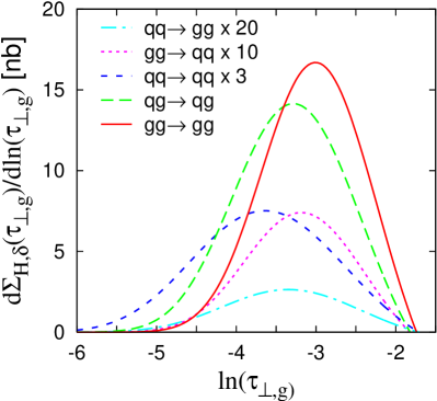
Figure 2: The differential cross section $d\Sigma_{\cal H}/d\ln\tau_{\perp,g}$ separated into the different hard-scattering channels.

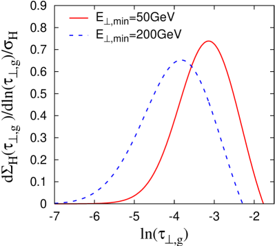
Figure 3: The differential cross section for $\tau_{\perp,g}$, summed over channels summed over channels, for two $E_{\perp,\min}$ cuts.

The resulting differential cross sections for different partonic scattering channels are shown in figure 3, where $q$ denotes a generic fermion (quark or antiquark) and $qg\to qg$ indicates any process with incoming fermion and gluon. They have been obtained by integrating over all hard events that satisfy the cuts discussed in section 2.3. The $d_{\ell}$ are redetermined for each hard configuration, since they depend on the kinematics of the event. While in table 1 the arbitrary reference hard scale was taken to be $\sqrt{\hat{s}}$, hereon, for the purposes of calculating differential cross sections we choose $Q$, as well as the renormalisation and factorisation scales, to be the sum of the two hardest jet transverse energies, which is closer to the virtuality of the exchanged parton in the hard scattering. Since the distributions are purely resummed, without the inclusion of the exact fixed-order contribution (matching, left to future work [53]), they are reliable only at small values of $\tau_{\perp,g}$. For $\tau_{\perp,g}\sim 1$, the differential cross sections are negative, this being a reflection of a breakdown of the resummation approach in that region.

At small $\tau_{\perp,g}$ the differential cross sections of fig. 3 have somewhat different shapes for the various hard-scattering channels ($\delta$). This is a consequence of the different colour factors multiplying the LL terms in eq. (7), the LL contribution being larger for channels with more hard gluons — such channels tend to radiate more, so the distribution is peaked at larger values of $\tau_{\perp,g}$.

Combining the different hard-scattering channels, one obtains the full resummed distribution, fig. 3. In section 2.2 we discussed the consequences of limited experimental rapidity coverage for comparisons between (fully global) theory and (partially global) data. The main result was that the resummation remains valid, in the range limited by eq. (10), which here translates to $L\lesssim\eta_{\max}$. A subtlety arises in the translation between $\tau_{\perp,g}$ and the value of $L$: as discussed in appendix A, in eq. (5) we resum not $\ln 1/\tau_{\perp,g}$ but actually $\ln 1/(X\tau_{\perp,g})$, where $X$ is chosen so as to cancel the average value of $d_{\ell}g_{\ell}(\phi)$. For the hard events satisfying the cuts in section 2.3 this corresponds to $X\simeq 5$. This is a convention, adopted from $e^{+}e^{-}$ [54] and DIS [40], intended to minimise spurious subleading logarithms associated with the potentially arbitrary normalisation of one’s observable. Since for the discussion of section 2.2, it is $L\equiv\ln 1/(X\tau_{\perp,g})$ that determines the maximum value of rapidity that is relevant in the resummation, eq. (10) should be rewritten

$$\ln v\gtrsim-(a+b_{\ell})(\eta_{\max}+\langle\ln X\rangle)\,.$$ (13)

Assuming $\eta_{\max}\simeq 3.5$, one obtains the limit $\ln\tau_{\perp,g}\gtrsim-5$, suggesting that the distribution is nearly entirely in a region where the limited experimental rapidity reach should be unimportant. If however one goes to higher energies, such as $E_{\perp,1}>200\;\mathrm{GeV}$ as shown in fig. 3, channels with smaller colour factors start to dominate (e.g. $qq\to qq$), because one samples the parton distributions at higher $x$; this together with the smaller value of $\alpha_{{\textsc{s}}}$ leads to the $\tau_{\perp,g}$ distribution being dominated by lower values of the observable.

A final point regarding $\tau_{\perp,g}$ concerns its sensitivity to the underlying event. To parametrise this sensitivity it is useful, as was done in [12], to take a simple model [30] in which particles from the underlying event have a spectrum $dn^{(u.e.)}/dk_{\perp}d\eta$ that is independent of $\eta$ and of the underlying hard scattering process. Since $\tau_{\perp,g}$ is additive, and sensitive along the incoming legs to $k_{\perp}g_{1,2}(\phi)$ (see tab. 1), it receives a mean contribution from the underlying event

$$\langle\delta^{(u.e.)}\tau_{\perp,g}\rangle =\left(\int_{-\eta_{\max}}^{-\eta_{\max}}d\eta+{\cal{O}}\left(1\right)\right)\int dk_{\perp}\frac{d\phi}{2\pi}\frac{dn^{(u.e.)}}{d\eta dk_{\perp}}\frac{k_{\perp}g_{\ell}(\phi)}{E_{\perp,1}+E_{\perp,2}}$$ (14a)

$$=\frac{\langle k_{\perp}^{(u.e.)}\rangle\langle g_{1,2}(\phi)\rangle}{E_{\perp,1}+E_{\perp,2}}\left(2\eta_{\max}+{\cal{O}}\left(1\right)\right)\,,$$ (14b)

where $\langle k_{\perp}^{(u.e.)}\rangle$ is the mean transverse momentum per unit rapidity coming from the underlying event. The unspecified contribution of ${\cal{O}}\left(1\right)$ reflects the fact that for this qualitative discussion, we have not taken into account the details of the observable’s sensitivity to emissions close to the outgoing jets. Though the result is for the mean effect of the underlying event, expectations based on other studies of non-perturbative effects [55] suggest that the distribution of $\tau_{\perp,g}$ will simply be shifted by $\langle\delta^{(u.e.)}\tau_{\perp,g}\rangle$. Because of the proportionality to $\eta_{\max}$, the effect will be large, making $\tau_{\perp,g}$ a good observable for testing models of the underlying event. For example the effects of the underlying event could depend on the underlying hard scattering channel, and it might then be possible, from the event-shape distribution, to establish whether or not this is the case.

3.2 Thrust minor

Given the transverse thrust axis $\vec{n}_{T}$, one can define a directly global thrust minor,

$$T_{m,g}\equiv\frac{\sum_{i}|q_{xi}|}{\sum_{i}q_{\perp i}}\,,$$ (15)

where the $x$ direction is defined as that perpendicular to the beam and to the global transverse thrust axis, which together define the event plane. The thrust minor can be viewed as a measure of the out-of-plane momentum, and is quite similar to the observable resummed analytically in [12] for Drell-Yan plus jet production.

One can also normalise the thrust minor to $E_{\perp,1}+E_{\perp,2}$. This will not modify the resummation, but it will affect the distribution at values of $T_{m,g}$ of order $1$. (Such a change cannot be made for the $T_{\perp,g}$, because it would destroy the positive definiteness of $\tau_{\perp,g}=1-T_{\perp,g}$).

leg $\ell$	$a_{\ell}$	$b_{\ell}$	$g_{\ell}(\phi)$	$d_{\ell}$
1	1	$0$	$|\sin\phi|$	$2/\sin\theta^{*}$
2	1	$0$	$|\sin\phi|$	$2/\sin\theta^{*}$
3	1	$0$	$|\sin\phi|$	$2/\sin\theta^{*}$
4	1	$0$	$|\sin\phi|$	$2/\sin\theta^{*}$

Table 2: Leg properties for $T_{m,g}$; $\langle\ln g_{\ell}(\phi)\rangle$, not shown, is $-\ln 2$ for all legs.

The main difference between the thrust minor and the transverse thrust concerns the properties of the outgoing legs, which for $T_{m,g}$ have $b_{\ell}=0$ (table 2). Referring to eq. (7), one sees that this implies larger double logarithms than for $\tau_{\perp,g}$. Additionally, the dependence on multiple emissions is more complex, $T_{m,g}$ not having the simple property of additivity, so it is necessary to calculate ${\cal{F}}(R^{\prime})$ numerically. The result, shown in fig. 5, is similar (though not identical) for all hard-scattering channels, and uniformly below $1$, which is indicative of the fact that multiple emissions increase the value of the observable relative to a single emission. We also note that the function ${\cal{F}}$ does not depend on the Born momenta ${\cal B}$, as can be verified numerically.

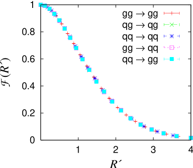
Figure 4: The ${\cal{F}}(R^{\prime})$ function for $T_{m,g}$.

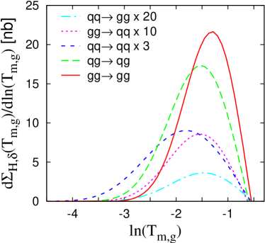
Figure 5: The distribution of $T_{m,g}$ in various hard-scattering channels.

The larger double logarithms ($b_{3,4}=0$) and the larger coefficient $d_{\ell}$ (together with the larger average value of $g_{\ell}(\phi)$) all contribute to $T_{m,g}$ having a distribution, fig. 5, that is dominated by considerably larger values of the observable than was the case for $\tau_{\perp,g}$. As a result the peak of the distribution is actually at only moderately small values of $T_{m,g}$, where fixed-order corrections (matching) may have a significant effect on the distribution.

The rescaling factor, $X$, in the resummation here (of $\ln 1/(XT_{m,g})$) is $X=1$. As a result the limited detector reach translates to a limit of applicability of the resummation $\ln T_{m,g}\gtrsim-\eta_{\max}$. The only channel that extends at all below our reference value of $\eta_{\max}\simeq 3.5$ is $qq\to qq$, which however, at these energies does not contribute significantly to the total distribution.

Finally we observe that the linearity of the definition of $T_{m,g}$ implies that it should have a sensitivity to the underlying event that is qualitatively quite similar to that of $\tau_{\perp,g}$, eqs. (14).

3.3 Three-jet resolution threshold

Clustering jet algorithms, such as the $k_{t}$-algorithm [50, 51, 57], involve a successive set of pairwise particle recombinations, so as to group particles into jets. These algorithms often involve a jet-resolution parameter, which determines the point at which to stop the pairwise recombination. The smaller the parameter, the larger the number of separate jets that gets resolved.

One of the most widely studied observables in $e^{+}e^{-}$ is the jet resolution threshold, $y_{23}$, above which the event is classified as having two jets, and below which it has three (or more) jets. Though an analogous threshold has been defined for going from $2+2$ to $2+3$ jet events with the longitudinally invariant $k_{t}$-algorithm in hadron-hadron collisions [50], it has received somewhat less attention. Resummed calculations [11] (to lower accuracy than is given here) and measurements [58] have been carried out only for the related problem of subjets within a single jet.

Jet threshold resolutions and jet rates are closely related since the integrated cross section $\Sigma_{\cal H}(y)$ for $y_{23}$ is equivalent to the cross section for having a two-jet event, given a jet resolution of $y$.

We will consider here just one variant of the $k_{t}$-algorithm (the exclusive form of that adopted for run II of the Tevatron [49]). Reference implementations of this and other schemes are available in [59].

1. One defines, for all $n$ final-state (pseudo)particles still in the event,

   $$d_{kB}=q_{\perp k}^{2}\,,$$ (16)

   and for each pair of final state particles

   $$d_{kl}=\min\{{q_{\perp k}^{2},q_{\perp l}^{2}}\}\left((\eta_{k}-\eta_{l})^{2}+(\phi_{k}-\phi_{l})^{2}\right)\,.$$ (17)

2. One determines the minimum over $k$ and $l$ of the $d_{kl}$ and the $d_{kB}$ and calls it $d^{(n)}$. If the smallest value is $d_{iB}$ then particle $q_{i}$ is included in the beam and eliminated from the final state particles. If the smallest value is $d_{ij}$ then particles $q_{i}$ and $q_{j}$ are recombined into a pseudoparticle (jet). A number of recombination procedures exist. We adopt the E-scheme, in which the particle four-momenta are simply added together,

   $$q_{ij}=q_{i}+q_{j}\,.$$ (18)

3. The procedure is repeated until only 3 pseudoparticles are left in the final state. The observable we resum is then

   $$y_{23}=\frac{1}{E_{\perp}^{2}}\max_{n\geq 3}\{d^{(n)}\}\>,$$ (19)

   where $E_{\perp}$ is defined by further clustering the event until only two jets remain and taking $E_{\perp}$ as the sum of the two jet transverse energies,

   $$E_{\perp}=E_{\perp,1}+E_{\perp,2}\,.$$ (20)

   The reason for considering $\max_{n\geq 3}\{d^{(n)}\}$ in eq. (19), instead of simply $d^{(3)}$, is that the recombination procedure is not necessarily monotonic in the $d^{(n)}$ [50], so that $n>m$ does not automatically imply $d^{(n)}<d^{(m)}$.

leg $\ell$	$a_{\ell}$	$b_{\ell}$	$g_{\ell}(\phi)$	$d_{\ell}$
1	2	$0$	1	$1/\sin^{2}\theta^{*}$
2	2	$0$	1	$1/\sin^{2}\theta^{*}$
3	2	$0$	1	$1/\sin^{2}\theta^{*}$
4	2	$0$	1	$1/\sin^{2}\theta^{*}$

Table 3: Leg properties for $y_{23}$.

From table 3 one sees that, for all legs, the effect of single emissions scales as the squared transverse momentum, without any rapidity or azimuthal dependence — in this respect the observable is similar to $y_{23}$ in $e^{+}e^{-}$.

An interesting theoretical feature of the hadronic $y_{23}$ concerns ${\cal{F}}$, fig. 7. In contrast to the transverse thrust and thrust minor cases, ${\cal{F}}(R^{\prime})$ has a strong dependence on the scattering channel. It seems that along the outgoing legs, multiple subjets can combine together before being combined with the main hard jet — this means that multiple emissions along an outgoing leg lead to a larger $y_{23}$ than a single emission, causing ${\cal{F}}$ to be smaller than $1$, as in $e^{+}e^{-}$ [36]. For incoming legs instead, subjets tend not to recombine together, so that the value of $y_{23}$ is determined exclusively by the hardest subjet. This type of situation leads to ${\cal{F}}(R^{\prime})=1$. The actual value for ${\cal{F}}$ then depends on the relative importance (colour factors) of the incoming and outgoing jets.

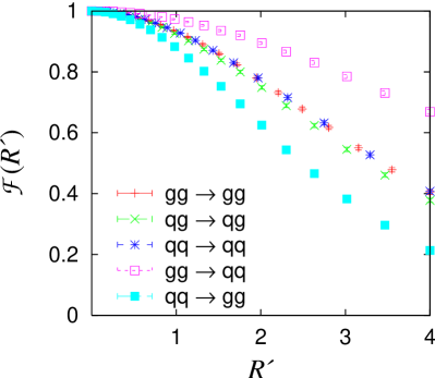
Figure 6: The ${\cal{F}}(R^{\prime})$ function for $y_{23}$.

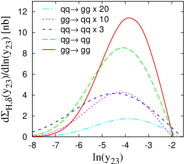
Figure 7: The distribution of $y_{23}$ in various hard-scattering channels.

Figure 7 shows the distribution of $y_{23}$ for different hard subprocesses. It extends to considerably smaller values than, say, $T_{m,g}$, the reason being that, from the point of view of LL contributions $y_{23}\sim T_{m,g}^{2}$. This suggests that the distribution of $\frac{1}{2}\ln y_{23}$ should be comparable to that of $\ln T_{m,g}$. One sees that to some extent this is the case, though the $y_{23}$ distribution is somewhat wider than would be expected based on this argument. This is a consequence of the larger suppression that $T_{m,g}$ receives from its ${\cal{F}}(R^{\prime})$ (note that at a given value of $y_{23}\sim T_{m,g}^{2}$, the definition of $R^{\prime}$ is such that $R^{\prime}_{y_{23}}=\mbox{\small$\frac{1}{2}$}R^{\prime}_{T_{m,g}}$).

The fact that $y_{23}\sim T_{m,g}^{2}$ is important also from the point of view of the impact of the limited experimental rapidity reach, since the range in which the cut can be ignored theoretically is $\ln y_{23}\gtrsim-2\eta_{\max}$. One sees that for $\eta_{\max}=3.5$, this includes most of the distribution, except in the $qq\to qq$ channel, which extends a little beyond.

While perturbatively $y_{23}$ and $T_{m,g}^{2}$ are similar, they should have very different sensitivities to non-perturbative physics. It is already known that in $e^{+}e^{-}$, $k_{t}$-type jet algorithms are relatively insensitive to non-perturbative effects. The same should be true also of the hadronic $y_{23}$ — for example, the fact that along incoming legs it is the hardest subjet that dominates, means that unlike $T_{m,g}$, $y_{23}$ does not ‘collect’ non-perturbative contributions from the whole range of $|\eta|<\eta_{\max}$, but rather just from a limited region around the hardest subjet.

4 Observables with exponentially suppressed forward terms

While the observables given above could be easily defined in a ‘global’ manner, other jet observables, such as jet masses or broadenings, are more naturally defined just in terms of a central region, or of the two leading jets. As a result they are usually not global, which prevents them from being resummed with current automated approaches such as caesar.

One solution to this problem is to explicitly add to them a term sensitive to emissions along the beam direction, so as to render them global. If we add just the $q_{\perp i}$, we will obtain observables whose incoming legs have rather similar properties to the transverse thrust or the thrust minor, in particular with regards to their sensitivity to the underlying event and to relevance of the experimental $\eta_{\max}$ cutoff.

Instead we add a contribution, $\sim q_{\perp i}e^{-|\eta_{i}|}$, with an exponential suppression in the forward direction. This will usually lead to observables having $b_{\ell}=a$ on the incoming legs, which doubles the range of $L$, eq. (10), in which the resummed predictions are insensitive to $\eta_{\max}$. Such observables will usually also have a reduced sensitivity to the underlying event, since the integral eq. (14a) will converge rapidly in $\eta$ giving a result of order $\langle k_{\perp}^{(u.e.)}\rangle/(E_{\perp,1}+E_{\perp,2})$, without any $\eta_{\max}$ enhancement.

Before defining such observables, let us first discuss the central region, ${\cal{C}}$, in which the ‘main’ event shape (for example the sum of jet masses) will be measured. Various options are possible, for example taking all particles in the two hardest jets; or taking all particles having $|\eta_{i}|<\eta_{c}+\delta\eta$, where $\eta_{c}$ specifies the region in which the two hardest jets should lie (section 2.3), while $\delta\eta$ extends this region, so as to ensure that all selected jets are well contained within ${\cal{C}}$. For implementation in caesar, we have used this second definition, with $\delta\eta=0.4$, though it should be noted that since our final variables will be global, the NLL resummed results are actually independent of the precise definition of ${\cal{C}}$.

Having established ${\cal{C}}$, we then introduce the mean transverse-energy weighted rapidity, $\eta_{\cal{C}}$, of the central region,

$$\eta_{\cal{C}}=\frac{1}{Q_{\perp,{\cal{C}}}}\sum_{i\in{\cal{C}}}\eta_{i}\,q_{\perp i}\,,\qquad\quad Q_{\perp,{\cal{C}}}=\sum_{i\in{\cal{C}}}q_{\perp i}\,,$$ (21)

and define the exponentially suppressed forward term,

$${\cal{E}}_{\cal{\bar{C}}}=\frac{1}{Q_{\perp,{\cal{C}}}}\sum_{i\notin{\cal{C}}}q_{\perp i}\,e^{-|\eta_{i}-\eta_{\cal{C}}|}\,,$$ (22)

such that it is invariant with respect to longitudinal boosts (modulo the dependence of ${\cal{C}}$ itself on boosts). We are now in a position to define some observables.

4.1 Transverse thrust, minor and jet resolution

Transverse thrust.

Let us first define a thrust similar to that of section 3.1, but only in terms of the particles in ${\cal{C}}$,

$$T_{\perp,{\cal{C}}}\equiv\max_{\vec{n}_{T,{\cal{C}}}}\frac{\sum_{i\in{\cal{C}}}|{\vec{q}}_{\perp i}\cdot{\vec{n}_{T,{\cal{C}}}}|}{Q_{\perp,{\cal{C}}}}\,,\qquad\quad\tau_{\perp,{\cal{C}}}\equiv 1-T_{\perp,{\cal{C}}}\,.$$ (23)

leg $\ell$	$a_{\ell}$	$b_{\ell}$	$g_{\ell}(\phi)$	$d_{\ell}$
1	$1$	$1$	1	$1/\sin\theta^{*}$
2	$1$	$1$	1	$1/\sin\theta^{*}$
3	$1$	$1$	$\sin^{2}\phi$	$1/\sin^{2}\theta^{*}$
4	$1$	$1$	$\sin^{2}\phi$	$1/\sin^{2}\theta^{*}$

Table 4: Leg properties for $\tau_{\perp,{\cal{E}}}$.

We then add the contribution ${\cal{E}}_{\cal{\bar{C}}}$ with the dependence on the forward emission,

$$\tau_{\perp,{\cal{E}}}\equiv\tau_{\perp,{\cal{C}}}+{\cal{E}}_{{\cal{\bar{C}}}}\,,$$ (24)

to obtain a global observable, the resulting leg properties being shown in table 4. One sees that for the outgoing legs, they coincide with those of table 1 for $\tau_{\perp,g}$, while for the incoming legs $b_{\ell}=1$, as expected. Like $\tau_{\perp,g}$, the observable is additive, so ${\cal{F}}$ is known analytically.

We could at this point continue the discussion for $\tau_{\perp,{\cal{E}}}$ along lines similar to those for the observables given above. Since, however, one can imagine introducing quite a few further observables, we prefer from now on to concentrate on just a subset of them, so as to illustrate interesting new features. Accordingly we refer the reader to detailed web pages [62] for further information about $\tau_{\perp,{\cal{E}}}$, as well as analogous extensions of the thrust minor,

$$T_{m,{\cal{C}}}\equiv\frac{1}{Q_{\perp,{\cal{C}}}}\sum_{i\in{\cal{C}}}|q_{xi}|\,,\qquad\quad T_{m,{\cal{E}}}=T_{m,{\cal{C}}}+{\cal{E}}_{{\cal{\bar{C}}}}\,,$$ (25)

(because of kinematic recoil, it turns out that $T_{m,{\cal{C}}}$ is global, and $T_{m,{\cal{E}}}$ has $b_{1,2}=0$ and identical resummation properties to $T_{m,{\cal{C}}}$); and the three-jet resolution threshold, with $y_{23,{\cal{C}}}$ defined by the algorithm of section 3.3 applied only to the final state particles in ${\cal{C}}$ (and the beam) and

$$y_{23,{\cal{E}}}\equiv y_{23,{\cal{C}}}+{\cal{E}}_{\cal{\bar{C}}}^{2}\,.$$ (26)

Note that it is necessary to add ${\cal{E}}_{\cal{\bar{C}}}^{2}$ here (rather than ${\cal{E}}_{\cal{\bar{C}}}$), so as to ensure the continuous globalness of the observable, $a_{1}=a_{2}=a_{3}=a_{4}$.

Let us now concentrate in more detail on some observables that are more naturally defined without explicit reference to a central region.

4.2 Jet masses

Having determined a (central) transverse thrust axis $\vec{n}_{T,{\cal{C}}}$ as above, one can separate the central region ${\cal{C}}$ into an up part ${\cal{C}}_{U}$ consisting of all particles in ${\cal{C}}$ with $\vec{p}_{\perp}\cdot\vec{n}_{T,{\cal{C}}}>0$ and a down part ${\cal{C}}_{D}$, particles in ${\cal{C}}$ with $\vec{p}_{\perp}\cdot\vec{n}_{T,{\cal{C}}}<0$. If ${\cal{C}}$ is taken to be made up of all particles in the two hardest jets, one can also define ${\cal{C}}_{U}$ and ${\cal{C}}_{D}$ as consisting of the two jets separately. Such an alternative definition should not change any of the NLL resummed predictions for the global variables, and may actually help to minimise subleading (NNLL) corrections.

One then defines, in analogy with $e^{+}e^{-}$ [63], the normalised squared invariant masses of the two regions

$$\rho_{X,{\cal{C}}}\equiv\frac{1}{Q_{\perp,{\cal{C}}}^{2}}\left(\sum_{i\in{\cal{C}}_{X}}q_{i}\right)^{2}\,,\qquad X=U,D\,,$$ (27)

from which one can obtain a (non-global) central sum of masses and heavy-mass,

$$\rho_{S,{\cal{C}}}\equiv\rho_{U,{\cal{C}}}+\rho_{D,{\cal{C}}}\,,\qquad\quad\rho_{H,{\cal{C}}}\equiv\max\{\rho_{U,{\cal{C}}},\rho_{D,{\cal{C}}}\}\,,$$ (28)

together with versions that include the addition of the exponentially-suppressed forward term,

$$\rho_{S,{\cal{E}}}\equiv\rho_{S,{\cal{C}}}+{\cal{E}}_{{\cal{\bar{C}}}}\,,\qquad\quad\rho_{H,{\cal{E}}}\equiv\rho_{H,{\cal{C}}}+{\cal{E}}_{{\cal{\bar{C}}}}\,.$$ (29)

leg $\ell$	$a_{\ell}$	$b_{\ell}$	$g_{\ell}(\phi)$	$d_{\ell}$
1	$1$	$1$	1	$1/\sin\theta^{*}$
2	$1$	$1$	1	$1/\sin\theta^{*}$
3	$1$	$1$	1	$1/\sin^{2}\theta^{*}$
4	$1$	$1$	1	$1/\sin^{2}\theta^{*}$

Table 5: Leg properties for $\rho_{S,{\cal{E}}}$ (and $\rho_{H,{\cal{E}}}$).

The single-emission leg properties for $\rho_{S,{\cal{E}}}$ and $\rho_{H,{\cal{E}}}$ are identical (even beyond the soft-collinear limit), and quite similar to those of $\tau_{\perp,{\cal{E}}}$ except for the lack of azimuthal dependence on the outgoing legs. The sum of squared masses, $\rho_{S,{\cal{E}}}$, is an additive observable, so ${\cal{F}}(R^{\prime})$ is given by eq. (12), while for the heavy-mass it needs to be computed numerically (and decreases for increasing $R^{\prime}$).

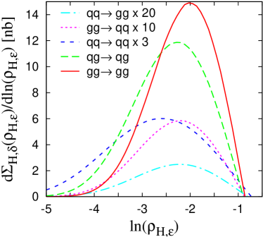
Figure 8: The distribution of $\rho_{H,{\cal{E}}}$ in the different hard-scattering channels.

The resummed distribution for $\rho_{H,{\cal{E}}}$ is shown, channel-by-channel in fig. 8. Compared, say, to an observable like $T_{m,g}$, the distributions extend to relatively low values, a consequence of the smaller LL terms (since $b=a$). However, as mentioned at the beginning of this section, the fact that $b_{1,2}=a=1$ means that the limit of applicability of the resummation, in the presence of an experimental rapidity cut, is given by $\ln\rho_{H,{\cal{E}}}\gtrsim-2\eta_{\max}$. Thus all channels for the distribution are comfortably contained within this region.

4.3 Jet Broadenings

With the same division into up and down regions as for the jet masses, one can define jet broadenings. To do so in a boost-invariant manner, one first introduces rapidities and azimuthal angles of axes for the up and down regions,

$$\eta_{X,{\cal{C}}}\equiv\frac{\sum_{i\in{\cal{C}}_{X}}q_{\perp i}\eta_{i}}{\sum_{i\in{\cal{C}}_{X}}q_{\perp i}}\,,\qquad\phi_{X,{\cal{C}}}\equiv\frac{\sum_{i\in{\cal{C}}_{X}}q_{\perp i}\phi_{i}}{\sum_{i\in{\cal{C}}_{X}}q_{\perp i}}\,,\qquad X=U,D\,,$$ (30)

and defines broadenings for the two regions,

$$B_{X,{\cal{C}}}\equiv\frac{1}{2Q_{\perp,{\cal{C}}}}\sum_{i\in{\cal{C}}_{X}}q_{\perp i}\sqrt{(\eta_{i}-\eta_{X,{\cal{C}}})^{2}+(\phi_{i}-\phi_{X,{\cal{C}}})^{2}}\,,\qquad X=U,D\,,$$ (31)

from which one can obtain central total and wide-jet broadenings,

$$B_{T,{\cal{C}}}\equiv B_{U,{\cal{C}}}+B_{D,{\cal{C}}}\,,\qquad\quad B_{W,{\cal{C}}}\equiv\max\{B_{U,{\cal{C}}},B_{D,{\cal{C}}}\}\,.$$ (32)

Adding the exponentially-suppressed forward terms gives global observables,

$$B_{T,{\cal{E}}}\equiv B_{T,{\cal{C}}}+{\cal{E}}_{{\cal{\bar{C}}}}\,,\qquad B_{W,{\cal{E}}}\equiv B_{W,{\cal{C}}}+{\cal{E}}_{{\cal{\bar{C}}}}\,.$$ (33)

leg $\ell$	$a_{\ell}$	$b_{\ell}$	$g_{\ell}(\phi)$	$d_{\ell}$
1	$1$	$1$	1	$1/\sin\theta^{*}$
2	$1$	$1$	1	$1/\sin\theta^{*}$
3	$1$	$0$	1	$1/\sin\theta^{*}$
4	$1$	$0$	1	$1/\sin\theta^{*}$

Table 6: Leg properties for $B_{T,{\cal{E}}}$ (and $B_{W,{\cal{E}}}$).

The single-emission properties of these two observables are identical and are shown in table 6. In both cases ${\cal{F}}(R^{\prime})$ needs to be calculated numerically, and it decreases with increasing $R^{\prime}$ (more strongly for $B_{T,{\cal{E}}}$).

The distribution for $B_{W,{\cal{E}}}$, separated into channels, is shown in fig. 10. As expected from the different double logarithmic structure for the outgoing legs, the $B_{W,{\cal{E}}}$ distributed is centred at larger values of the observable than $\rho_{H,{\cal{E}}}$. This can be seen clearly also from fig. 10 which shows both distributions, summed over channels for two different $E_{\perp,\min}$ cuts. Since a limited experimental rapidity translates into an allowed range of the observable’s value $\ln v\gtrsim-2\eta_{\max}$, we see that the distributions for both $\rho_{H,{\cal{E}}}$ and $B_{W,{\cal{E}}}$ are within the theoretically reliable region. The same statement applies to most of the other observables defined in this section.

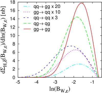
Figure 9: The distribution of $B_{W,{\cal{E}}}$ for separate hard-scattering channels.

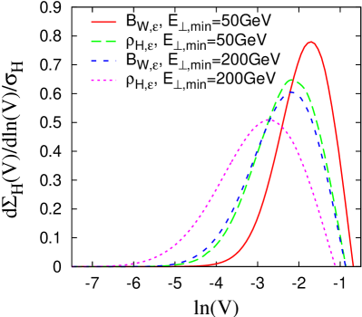
Figure 10: The distributions for $\rho_{H,{\cal{E}}}$ and $B_{W,{\cal{E}}}$, summed over channels, for two $E_{\perp,\min}$ cuts.

5 Indirectly global observables

We call ‘indirectly global’ those observables that explicitly measure only a subset of the particles in an event, but are nevertheless indirectly sensitive to the remaining emissions, typically through recoil. Previously studied examples include certain DIS Breit-frame event shapes, such as the current-hemisphere broadening with respect to the photon axis [65] or one of the variants of the thrust, $\tau_{zQ}$ [66].

Indirectly global observables have the advantage that they can be defined purely in terms of particles in the central region ${\cal{C}}$, while still remaining global. This eliminates potential problems associated with the limited experimental reach in rapidity.

To construct an indirectly global observable, one takes one of the ‘central’, non-global observables of the previous section, and then adds to it some second ‘recoil’ quantity, also defined only in terms of the momenta of ${\cal{C}}$, but that is sensitive to the emissions outside ${\cal{C}}$. An example of such a ‘recoil’ quantity is the 2-dimensional vector sum of the transverse momenta in ${\cal{C}}$,

$${\cal{R}}_{\perp,{\cal{C}}}\equiv\frac{1}{Q_{\perp,{\cal{C}}}}\left|\sum_{i\in{\cal{C}}}{\vec{q}}_{\perp i}\right|\,,$$ (34)

(with $Q_{\perp,{\cal{C}}}$ defined in eq. (21)) which, by conservation of momentum, is equal to (minus) the vector sum of the transverse momenta outside ${\cal{C}}$. Thus we obtain a whole series of ‘indirectly global’ event shapes, whose definitions are similar to those of section 4, but with ${\cal{E}}_{{\cal{\bar{C}}}}$ replaced by ${\cal{R}}_{\perp,{\cal{C}}}$:

$$\tau_{\perp,{\cal{R}}} \,\equiv\,\tau_{\perp,{\cal{C}}}+{\cal{R}}_{\perp,{\cal{C}}}\,,$$ (35a)

$$T_{m,{\cal{R}}} \,\equiv\,T_{m,{\cal{C}}}+{\cal{R}}_{\perp,{\cal{C}}}\,,$$ (35b)

$$y_{23,{\cal{R}}} \,\equiv\,y_{23,{\cal{C}}}+{\cal{R}}_{\perp,{\cal{C}}}^{2}\,,$$ (35c)

$$\rho_{S,{\cal{R}}} \,\equiv\,\rho_{S,{\cal{C}}}+{\cal{R}}_{\perp,{\cal{C}}}\,,\;\,\qquad\quad\rho_{H,{\cal{R}}}\,\equiv\,\rho_{H,{\cal{C}}}+{\cal{R}}_{\perp,{\cal{C}}}\,,$$ (35d)

$$B_{T,{\cal{R}}} \,\equiv\,B_{T,{\cal{C}}}+{\cal{R}}_{\perp,{\cal{C}}}\,,\qquad\quad B_{W,{\cal{R}}}\,\equiv\,B_{W,{\cal{C}}}+{\cal{R}}_{\perp,{\cal{C}}}\,.$$ (35e)

Experimentally, we envisage that the main difficulty that will arise specifically for this class of observables is the accurate determination of ${\cal{R}}_{\perp,{\cal{C}}}$, since it involves a cancellation between hard momenta. The extent to which this ‘missing transverse momentum’ can be well measured will determine the extent to which it will be possible to study the region of low event-shape values.

leg $\ell$	$a_{\ell}$	$b_{\ell}$	$g_{\ell}(\phi)$	$d_{\ell}$
1	$1$	$0$	1	$1/\sin\theta^{*}$
2	$1$	$0$	1	$1/\sin\theta^{*}$
3	$1$	$1$	$\sin^{2}\phi$	$1/\sin^{2}\theta^{*}$
4	$1$	$1$	$\sin^{2}\phi$	$1/\sin^{2}\theta^{*}$

Table 7: Leg properties for $\tau_{\perp,{\cal{R}}}$.

leg $\ell$	$a_{\ell}$	$b_{\ell}$	$g_{\ell}(\phi)$	$d_{\ell}$
1	$1$	$0$	$(1\!+\!|\sin\phi|)/2^{*}$	$2/\sin\theta^{*}$
2	$1$	$0$	$(1\!+\!|\sin\phi|)/2^{*}$	$2/\sin\theta^{*}$
3	$1$	$0$	$|\sin\phi|$	$2/\sin\theta^{*}$
4	$1$	$0$	$|\sin\phi|$	$2/\sin\theta^{*}$

Table 8: Leg properties for $T_{m,{\cal{R}}}$; $\langle\ln g_{1,2}(\phi)\rangle=4G/\pi-2\ln 2$.

The single-emission properties for two of these observables are illustrated in tables 8 and 8. As expected, the outgoing legs have identical properties to the global variants of the observables. The incoming legs have $b_{\ell}=a$, and a simple calculation reveals that $d_{\ell}=1/\sin\theta$ and $g_{\ell}(\phi)=1$ for most observables, including $\tau_{\perp,{\cal{R}}}$. An exception is $T_{m,{\cal{R}}}$, for which there is an interplay between recoil dependence present (implicitly) in $T_{m,{\cal{C}}}$, and the additional ${\cal{R}}_{\perp,{\cal{C}}}$ term.

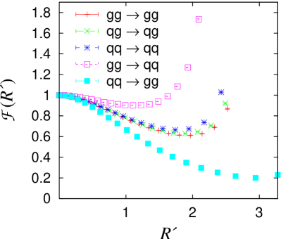
Figure 11: ${\cal{F}}(R^{\prime})$ for $\tau_{\perp,{\cal{R}}}$.

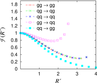
Figure 12: ${\cal{F}}(R^{\prime})$ for $T_{m,{\cal{R}}}$.

The ${\cal{F}}(R^{\prime})$ functions for $\tau_{\perp,{\cal{R}}}$ and $T_{m,{\cal{R}}}$ are shown in figures 12 and 12. For small values of $R^{\prime}$, ${\cal{F}}(R^{\prime})$ is below $1$, as for the observables discussed in the previous sections. However for sufficiently large $R^{\prime}$, ${\cal{F}}(R^{\prime})$ starts to increase and it has a divergence at some finite value of $R^{\prime}=R^{\prime}_{c}$. Such divergences are actually a well-understood phenomenon [65, 67], characteristic of observables for which contributions from multiple emissions can cancel. Schematically, they occur because for sufficiently large $R^{\prime}$ it becomes more favourable to suppress the value of the observable via cancellations between emissions than by Sudakov suppression, and the resulting change in parametric behaviour of $\Sigma_{\cal H}(v)$ cannot be represented as a subleading correction to a Sudakov resummation.

For the observables being discussed here, the cancellation is in the vector sum of transverse momenta. This being a two-dimensional cancellation, the divergence is located at $R^{\prime}_{1+2}=2$ [19, 65], where $R^{\prime}_{1+2}$ is the part of $R^{\prime}$ associated with the incoming legs. For cases where $R^{\prime}_{1+2}=\frac{1}{2}R^{\prime}$, such as the $gg\to gg$ channel for $T_{m,{\cal{R}}}$ then $R^{\prime}_{c}=4$. For the $gg\to qq$ scattering channel, in which $R^{\prime}$ comes mostly from the incoming legs, the divergence is at lower $R^{\prime}$. Furthermore for any given fixed channel, the divergence occurs earlier for the transverse thrust than for the minor, because the thrust has smaller LL terms, and accordingly a larger proportion of $R^{\prime}$ is associated with the incoming legs.

The divergence is a structure that appears even more strongly at yet higher orders (NNLL, …) and it could in principle be resummed. Technically speaking, one would have to carry out a $b$-space resummation [68] on the incoming legs, a ‘normal’ resummation for the outgoing legs, and include a non-global resummation [37] to deal with the dynamic discontinuous non-globalness [40] associated with the boundary of ${\cal{C}}$. This is technically rather challenging and so far the only such resummation [65], for a jet-broadening in DIS, neglected the non-global logarithms. The conclusion of that study (for a case in which $R^{\prime}_{c}=4$) was that the further resummation had negligible practical impact except in a region where the distribution was already very strongly suppressed.

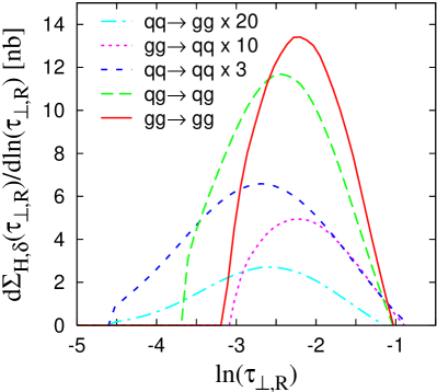
Figure 13: The distribution of $\tau_{\perp,{\cal{R}}}$ for separate hard-scattering channels.

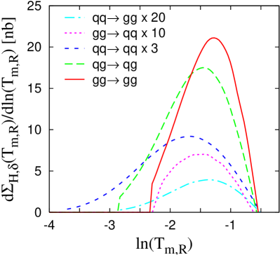
Figure 14: The distribution of $T_{m,{\cal{R}}}$ for separate hard-scattering channels.

We therefore follow the approach of [65] and consider the distributions for the observables without any additional resummation, figs. 14 and 14. The distributions are cut (somewhat arbitrarily) at the point where $R^{\prime}=7/8R^{\prime}_{c}$ — one sees that this corresponds to different values of $\ln v$, depending on the resummation channel. However for each channel most of the cross section is in the theoretically reliable region where the divergence can be ignored. We note that some problems do arise in the combination of channels with divergences at different points, notably from the point of view of establishing the region in which the sum over all channels is well estimated. The detailed discussion of this issue will be left to future work [53].

We conclude this section by observing that there are reasons to believe that these observables, though global, should have a relatively limited sensitivity to the underlying event. This is because in the sum of perturbative and ‘underlying-event’ contributions to ${\cal{R}}_{\perp,{\cal{C}}}$, after integration over azimuthal angles, the leading piece of the underlying event component averages to zero, leaving only a subleading component.

6 Conclusions

In this article we have defined and resummed a set of dijet event-shape observables and jet rates that are suitable for study at hadronic colliders, both from a theoretical and an experimental point of view. The principle issues that had to be reconciled were those of globalness, which greatly simplifies the resummed theoretical predictions, and of limited experimental reach in rapidity. At first sight these requirements seem contradictory, however we saw that it is possible to define several classes of observables which meet both criteria.

For a majority of the observables, the distribution is concentrated in a region where the limited experimental rapidity reach can be ignored in the resummed prediction. This is the case for nearly all the directly global observables of section 3 and those with exponentially suppressed forward terms, section 4, the latter having been specifically designed to be optimal in this respect. The observables of section 5, defined only in terms of particles in the central region, avoid the problem altogether, implementing globalness ‘indirectly’ via a recoil term (though this affects the validity of the resummation in a limited region of very small event-shape values).

The study of a range of observables, as presented here, would have been considerably more difficult without the help of the automated resummation tool, caesar. For brevity we omitted a range of further results [62]. Full phenomenological studies will necessitate also matching with fixed order calculations such as [13, 14, 15], some relevant issues for ‘practitioners’ having been discussed in appendix B.

One of the main reasons for examining several classes of observable (and a number of observables within each class) is that they have quite complementary sensitivities to different physics issues, both perturbative and non-perturbative. Possible studies include measurements of $\alpha_{{\textsc{s}}}$, tests of novel perturbative QCD colour evolution structures that arise in events with $4$-jet topology, and investigations into hadronisation effects and the properties of the underlying event. Overall, we believe that this represents a potentially far richer programme of investigations than has, for example, been carried out in $e^{+}e^{-}$ or DIS processes.

Acknowledgements

This paper has evolved from discussions with a number of colleagues, including in particular Leonard Christofek, Yuri Dokshitzer, Joey Huston, Pino Marchesini, Aurore Savoy-Navarro and Mike Seymour. We are grateful also the CERN and the IPPP, Durham for the use computing facilities. GPS would like to thank also the Fermilab theory group for hospitality while this article was being prepared.

Appendix A Scale choices

As discussed in [40, 65, 73], in a resummation at NLL accuracy there is an intrinsic ambiguity in the choice of the logarithm to be resummed, for instance instead of resumming

$$L=\ln\frac{1}{v}\,,$$ (36)

one could equally well want to resum

$$\bar{L}=\ln\frac{1}{Xv}\,,\qquad\mbox{with}\quad X={\cal{O}}\left(1\right)\,.$$ (37)

This alternative choice for the logarithm affects the functional form of the single-logarithmic terms, but not the overall answer at NLL. Changing $X$ allows one then to estimate the size of a specific class of higher order (NNLL) corrections. In two-jet event shapes, the default value for $X$ was chosen in a ‘natural’ way by requiring that the coefficient $G_{11}$, the ${\cal{O}}\left(\alpha_{{\textsc{s}}}\right)$ single logarithmic term, contained only terms due to hard collinear splitting. This corresponded to taking $X=1/d$ (usually $d_{1}=d_{2}\equiv d$ in $e^{+}e^{-}$) and ensured that one didn’t introduce large spurious subleading logarithms whose coefficients involved powers of $\ln d$, associated just with the overall (arbitrary) normalisation of the observable.

The equivalent procedure more generally would be to define $X$ so as to cancel the coefficient $d_{\ell}g_{\ell}(\phi)$ in eq. (6). The obvious difficulty though is that $d_{\ell}g_{\ell}(\phi)$ is not a constant — it depends on the hard leg $\ell$ and on the value of the azimuthal angle.

Inspecting the detailed resummation formulae, in particular eq. (3.6) of [19], one sees that the problem of the azimuthal dependence can be eliminated, insofar as the resummed result depends only on $\ln\bar{d}_{\ell}\equiv\ln d_{\ell}+\int\frac{d\phi}{2\pi}\ln g_{\ell}(\phi)$. Furthermore, for each leg (if all the $b_{\ell}$ values are the same), the term involving $\ln\bar{d}_{\ell}$ comes in with a weight proportional to the colour factor, $C_{\ell}$, of the leg. So for $X$ to cancel the coefficient $d_{\ell}g_{\ell}(\phi)$ on average, it suffices to take

$$\ln X=-\frac{1}{C_{T}}\sum_{\ell=1}^{n}\left(C_{\ell}\ln\bar{d}_{\ell}\right)\,,\qquad\quad C_{T}\equiv\sum_{\ell=1}^{n}C_{\ell}\,.$$ (38)

with $n$ the number of hard legs. This choice means however that $L$ is defined differently for different colour configurations, which while legitimate, may seem a little unnatural. In this study we therefore adopt a prescription for $X$, which is numerically almost indistinguishable from the choice in eq. (38), but does not have the unusual feature that the logarithm depends on the specific colour configuration,

$$\ln X=-\frac{1}{n}\sum_{\ell=1}^{n}\ln\bar{d}_{\ell}\,.$$ (39)

For situations in which all legs have the same colour factor, it is equivalent to eq. (38).

Appendix B Comparison to fixed order

A valuable cross-check on any resummed prediction is that its expansion to fixed order coincides with the logarithmically enhanced terms of exact fixed-order predictions. For $e^{+}e^{-}\to 2\;\mathrm{jets}$ and DIS $1+1\;\mathrm{jet}$ resummations, such checks have been carried out to NLO accuracy. The current status of the NLO codes suitable for NLO prediction of hadronic dijet event shapes is that NLOJET++ [13] is available publicly, while TRIRAD [15] can be requested from the authors.

We have carried out comparisons with NLOJET++. This turned out to be feasible at LO (for the $\alpha_{{\textsc{s}}}L^{2}$ and $\alpha_{{\textsc{s}}}L$ terms of $\Sigma_{\cal H}(v)/\sigma_{\cal H}$), while we encountered difficulties in obtaining a determination of the NLO contribution that was sufficiently accurate to enable a meaningful comparison with the expansion of the resummations. Nevertheless even the LO comparisons represent a non-trivial check of the resummations, in particular in view of the involved four-jet large-angle colour structure.

Fixed-order calculations are relevant not only as checks of the resummation, but more importantly for matching [39], so as to obtain predictions that are valid for large as well as small values of the observable. The matching also gives a partial improvement in the accuracy at small values of the observable, supplementing, for instance, eq. (5) with a term known as $C_{1}$, which depends on the momentum configuration and the channel,

$$f_{{\cal B},\delta}(v)=\left(1+C_{1,{\cal B},\delta}\frac{\alpha_{{\textsc{s}}}}{2\pi}+\ldots\right)\exp\left[Lg_{1,\delta}(\alpha_{{\textsc{s}}}L)+g_{2,{\cal B},\delta}(\alpha_{{\textsc{s}}}L)+\alpha_{{\textsc{s}}}g_{3,{\cal B},\delta}(\alpha_{{\textsc{s}}}L)+\cdots\right]\,,$$ (40)

where we have explicitly indicated the dependence of the $g_{n}(\alpha_{{\textsc{s}}}L)$ on the channel $\delta$ and (for $n\geq 2$) on the momentum configuration ${\cal B}$ (elsewhere this dependence has been left implicit).

The improvement in accuracy comes, for example, because the product of $C_{1,{\cal B},\delta}$ and the first term in the expansion of $Lg_{1,\delta}(\alpha_{{\textsc{s}}}L)$ helps to fix the $\alpha_{{\textsc{s}}}^{n}L^{2n-2}$ terms in the expansion of $f_{{\cal B},\delta}(v)$, or equivalently, after summing over channels and integrating over Born configurations, in $\Sigma_{\cal H}(v)/\sigma_{\cal H}$. Currently however, fixed-order programs are at best able to provide a weighted sum of $C_{1,{\cal B},\delta}$ values across all channels

$$\langle C_{1,{\cal B}}\rangle_{\delta}=\frac{\sum_{\delta}\frac{d\sigma_{\delta}}{d{\cal B}}C_{1,{\cal B},\delta}}{\sum_{\delta}\frac{d\sigma_{\delta}}{d{\cal B}}}\,.$$ (41)

Since different channels have different colour factors appearing in $Lg_{1,\delta}(\alpha_{{\textsc{s}}}L)$, the averaging over channels for $C_{1,{\cal B},\delta}$ means that one cannot reconstruct the full information for the sum of products of $C_{1,{\cal B},\delta}$ and $Lg_{1,\delta}(\alpha_{{\textsc{s}}}L)$

$$\langle\,C_{1,{\cal B}}\;Lg_{1}(\alpha_{{\textsc{s}}}L)\,\rangle_{\delta}\,\neq\,\langle C_{1,{\cal B}}\rangle_{\delta}\;\langle Lg_{1}(\alpha_{{\textsc{s}}}L)\rangle_{\delta}\,.$$ (42)

The fact that the $C_{1,{\cal B},\delta}$ are characteristics of the soft and collinear limit, means that they can in principle be unambiguously extracted channel-by-channel [53], enabling a proper average to be carried out. However the identification of the channel requires that one have information on the flavour of individual partons in the fixed-order calculation. Though such information is present in some form in existing fixed-order codes [13, 15], it is not, as far as we understand, available through the external ‘user’ interfaces to those codes. The availability of a method to access this information more straightforwardly would be of considerable help for the matching.

References

- [1] S. Bethke, Nucl. Phys. 121 (Proc. Suppl.) (2003) 74 [hep-ex/0211012].
- [2] S. Kluth et al., Eur. Phys. J. C 21 (2001) 199 [hep-ex/0012044] and references therein.
- [3] G. Marchesini, B. R. Webber, G. Abbiendi, I. G. Knowles, M. H. Seymour and L. Stanco, Comput. Phys. Commun. 67 (1992) 465; G. Corcella et al., J. High Energy Phys. 01 (2001) 010 [hep-ph/0011363].
- [4] T. Sjöstrand, Comput. Phys. Commun. 82 (1994) 74; T. Sjöstrand, P. Eden, C. Friberg, L. Lönnblad, G. Miu, S. Mrenna and E. Norrbin, Comput. Phys. Commun. 135 (2001) 238 [hep-ph/0010017].
- [5] L. Lönnblad, Comput. Phys. Commun. 71 (1992) 15.
- [6] P. Abreu et al. (DELPHI Collaboration), Z. Physik C 73 (1996) 11.
- [7] M. Beneke, Phys. Rept. 317 (1999) 1 [hep-ph/9807443].
- [8] M. Dasgupta and G. P. Salam, J. Phys. G 30 (2004) R143 [hep-ph/0312283].
- [9] F. Abe et al. [CDF Collaboration], Phys. Rev. D 44 (1991) 601.
- [10] I. A. Bertram [D0 Collaboration], Acta Phys. Polon. B 33 (2002) 3141.
- [11] J. R. Forshaw and M. H. Seymour, J. High Energy Phys. 09 (1999) 009 [hep-ph/9908307].
- [12] A. Banfi, G. Marchesini, G. Smye and G. Zanderighi, J. High Energy Phys. 08 (2001) 047 [hep-ph/0106278].
- [13] Z. Nagy, Phys. Rev. Lett. 88 (2002) 122003 [hep-ph/0110315].
- [14] Z. Nagy, Phys. Rev. D 68 (2003) 094002 [hep-ph/0307268].
- [15] W. B. Kilgore and W. T. Giele, hep-ph/0009193; Phys. Rev. D 55 (1997) 7183 [hep-ph/9610433].
- [16] J. Campbell and R. K. Ellis, Phys. Rev. D 65 (2002) 113007 [hep-ph/0202176].
- [17] R. Bonciani, S. Catani, M. L. Mangano and P. Nason, Phys. Lett. B 575 (2003) 268 [hep-ph/0307035].
- [18] A. Banfi, G. P. Salam and G. Zanderighi, Phys. Lett. B 584 (2004) 298 [hep-ph/0304148].
- [19] A. Banfi, G. P. Salam and G. Zanderighi, hep-ph/0407286.
-
[20]
R. K. Ellis, G. Marchesini and B. R. Webber,
Nucl. Phys. B 286 (1987) 643
[Erratum ibid. B 294 (1987) 1180];
Y. L. Dokshitzer, V. A. Khoze and S. I. Troyan, Adv. Ser. Direct. High Energy Phys. 5 (1988) 241. - [21] J. Botts and G. Sterman, Nucl. Phys. B 325 (1989) 62.
- [22] N. Kidonakis and G. Sterman, Phys. Lett. B 387 (1996) 867; Nucl. Phys. B 505 (1997) 321 [hep-ph/9705234].
- [23] N. Kidonakis, G. Oderda and G. Sterman, Nucl. Phys. B 531 (1998) 365 [hep-ph/9803241].
- [24] G. Oderda, Phys. Rev. D 61 (2000) 014004 [hep-ph/9903240].
- [25] N. Kidonakis and J. F. Owens, Phys. Rev. D 63 (2001) 054019 [hep-ph/0007268].
- [26] R. B. Appleby and M. H. Seymour, J. High Energy Phys. 09 (2003) 056 [hep-ph/0308086].
- [27] A. V. Manohar and M. B. Wise, Phys. Lett. B 344 (1995) 407 [hep-ph/9406392]; B. R. Webber, Phys. Lett. B 339 (1994) 148 [hep-ph/9408222]; Y. L. Dokshitzer and B. R. Webber, Phys. Lett. B 352 (1995) 451 [hep-ph/9504219]; M. Beneke and V. M. Braun, Nucl. Phys. B 454 (1995) 253 [hep-ph/9506452]; R. Akhoury and V. I. Zakharov, Phys. Lett. B 357 (1995) 646 [hep-ph/9504248].
- [28] G. P. Korchemsky and G. Sterman, Nucl. Phys. B 437 (1995) 415 [hep-ph/9411211]; G. P. Korchemsky and G. Sterman, Nucl. Phys. B 555 (1999) 335 [hep-ph/9902341]; E. Gardi and J. Rathsman, Nucl. Phys. B 609 (2001) 123 [hep-ph/0103217].
- [29] R. D. Field and R. P. Feynman, Phys. Rev. D 15 (1977) 2590; Nucl. Phys. B 136 (1978) 1; R. P. Feynman, ‘Photon-hadron interactions’, W. A. Benjamin, New York (1972); B. R. Webber, in proceedings of the ‘Summer School on Hadronic Aspects of Collider Physics’, Zuoz, Switzerland, 1994, hep-ph/9411384.
- [30] G. Marchesini and B. R. Webber, Phys. Rev. D 38 (1988) 3419.
- [31] D. Acosta et al. [CDF Collaboration], hep-ex/0404004.
- [32] A. Banfi, G. Marchesini, Yu. L. Dokshitzer and G. Zanderighi, J. High Energy Phys. 07 (2000) 002 [hep-ph/0004027]; J. High Energy Phys. 05 (2001) 040 [hep-ph/0104162].
- [33] A. Banfi, G. Marchesini, G. Smye and G. Zanderighi, J. High Energy Phys. 11 (2001) 066 [hep-ph/0111157].
- [34] A. Banfi, G. Marchesini and G. Smye, J. High Energy Phys. 04 (2002) 024 [hep-ph/0203150].
- [35] A. Banfi and M. Dasgupta, J. High Energy Phys. 01 (2004) 027 [hep-ph/0312108].
- [36] A. Banfi, G. P. Salam and G. Zanderighi, J. High Energy Phys. 01 (2002) 018 [hep-ph/0112156].
- [37] M. Dasgupta and G. P. Salam, Phys. Lett. B 512 (2001) 323 [hep-ph/0104277].
- [38] J. C. Collins, D. E. Soper and G. Sterman, Nucl. Phys. B 250 (1985) 199.
- [39] S. Catani, L. Trentadue, G. Turnock and B. R. Webber, Nucl. Phys. B 407 (1993) 3.
- [40] M. Dasgupta and G. P. Salam, J. High Energy Phys. 08 (2002) 032 [hep-ph/0208073].
- [41] R. Blair et al. [CDF-II Collaboration], “The CDF-II detector: Technical design report,” FERMILAB-PUB-96-390-E.
- [42] V. M. Abazov et al. [D0 Collaboration], “Run IIb upgrade technical design report,” FERMILAB-PUB-02-327-E; J. Ellison [D0 Collaboration], “The D0 detector upgrade and physics program,” Prepared for 15th International Workshop on High-Energy Physics and Quantum Field Theory (QFTHEP 2000), Tver, Russia, 14-20 Sep 2000.
- [43] J. Huston, private communication.
- [44] L. Christofek, private communication.
- [45] ATLAS Technical Proposal, CERN/LHCC/94-43, LHCC/P2, 15 December 1994.
- [46] HCAL Technical Design Report, CERN/LHCC 97-31, CMS TDR 2, 20 June 1997.
- [47] M. Klasen and G. Kramer, Phys. Lett. B 366 (1996) 385 [hep-ph/9508337].
- [48] S. Frixione and G. Ridolfi, Nucl. Phys. B 507 (1997) 315 [hep-ph/9707345].
- [49] G. C. Blazey et al., hep-ex/0005012.
- [50] S. Catani, Y. L. Dokshitzer, M. H. Seymour and B. R. Webber, Nucl. Phys. B 406 (1993) 187.
- [51] S. D. Ellis and D. E. Soper, Phys. Rev. D 48 (1993) 3160 [hep-ph/9305266].
- [52] J. Pumplin et al., J. High Energy Phys. 07 (2002) 012 [hep-ph/0201195].
- [53] A. Banfi, G. P. Salam and G. Zanderighi, work in progress.
- [54] S. Catani and B. R. Webber, Phys. Lett. B 427 (1998) 377 [hep-ph/9801350].
- [55] Y. L. Dokshitzer and B. R. Webber, Phys. Lett. B 404 (1997) 321 [hep-ph/9704298].
- [56] D. P. Barber et al. [MARK-J COLLABORATION Collaboration], Phys. Rept. 63 (1980) 337.
- [57] S. Catani, Yu. L. Dokshitzer, M. Olsson, G. Turnock and B. R. Webber, Phys. Lett. B 269 (1991) 432.
- [58] V. M. Abazov et al. [D0 Collaboration], Phys. Rev. D 65 (2002) 052008 [hep-ex/0108054].
- [59] J. M. Butterworth, J. P. Couchman, B. E. Cox and B. M. Waugh, Comput. Phys. Commun. 153 (2003) 85 [hep-ph/0210022].
- [60] C. F. Berger, T. Kucs and G. Sterman, Int. J. Mod. Phys. A 18 (2003) 4159 [hep-ph/0212343]; Phys. Rev. D 68 (2003) 014012 [hep-ph/0303051].
- [61] C. F. Berger and G. Sterman, J. High Energy Phys. 09 (2003) 058 [hep-ph/0307394].
- [62] Analyses and resummed results for a large number of observables are available from http://qcd-caesar.org/ .
- [63] L. Clavelli, Phys. Lett. B 85 (1979) 111; T. Chandramohan and L. Clavelli, Nucl. Phys. B 184 (1981) 365; L. Clavelli and D. Wyler, Phys. Lett. B 103 (1981) 383.
- [64] G. P. Salam and D. Wicke, J. High Energy Phys. 05 (2001) 061 [hep-ph/0102343].
- [65] M. Dasgupta and G. P. Salam, Eur. Phys. J. C 24 (2002) 213 [hep-ph/0110213].
- [66] V. Antonelli, M. Dasgupta and G. P. Salam, J. High Energy Phys. 02 (2000) 001 [hep-ph/9912488].
- [67] P. E. L. Rakow and B. R. Webber, Nucl. Phys. B 187 (1981) 254.
- [68] G. Parisi and R. Petronzio, Nucl. Phys. B 154 (1979) 427.
- [69] Y. L. Dokshitzer, A. Lucenti, G. Marchesini and G. P. Salam, J. High Energy Phys. 05 (1998) 003 [hep-ph/9802381].
- [70] Y. L. Dokshitzer, G. Marchesini and G. P. Salam, Eur. Phys. J. Direct. C 1 (1999) 3 [hep-ph/9812487].
- [71] P. A. Movilla Fernandez, hep-ex/0209022.
- [72] T. Kluge, hep-ex/0310063.
- [73] R. W. L. Jones, M. Ford, G. P. Salam, H. Stenzel and D. Wicke, J. High Energy Phys. 12 (2003) 007 [hep-ph/0312016].