Principles of general final-state resummation and automated implementation

Abstract:

Next-to-leading logarithmic final-state resummed predictions have traditionally been calculated, manually, separately for each observable. In this article we derive NLL resummed results for generic observables. We highlight and discuss the conditions that the observable should satisfy for the approach to be valid, in particular continuous globalness and recursive infrared and collinear safety. The resulting resummation formula is expressed in terms of certain well-defined characteristics of the observable. We have written a computer program, caesar, which, given a subroutine for an arbitrary observable, determines those characteristics, enabling full automation of a large class of final-state resummations, in a range of processes.

1 Introduction

It is a well known feature of QCD, and gauge theories in general, that final-state properties of the bulk of events in high-energy collisions cannot be predicted by standard fixed-order perturbative calculations. The very concept of ‘bulk’, or ‘typical’ events implies that in the expression for their probability, each power of the formally small coupling, $\alpha_{{\textsc{s}}}$, is compensated by a coefficient of order $1/\alpha_{{\textsc{s}}}$. These large coefficients are generally associated with logarithms ($L$) of widely disparate scales in the problem, and fixed-order truncations of the perturbative series often give unreliable answers.

So it is necessary to reorganise the perturbative series in terms of sets of dominant logarithmically enhanced classes of terms, i.e. a class of leading logarithmic (LL) terms (which might for example go as $\alpha_{{\textsc{s}}}^{n}L^{2n}$), next-to-leading logarithmic (NLL) terms (e.g. $\alpha_{{\textsc{s}}}^{n}L^{2n-1}$) and so on. For an appropriate range of (large) values of the logarithm $L$, it can be shown that this resummed hierarchy is convergent, i.e. that NLL terms are truly smaller than LL terms, and that next-to-next-to-leading logarithms (NNLL) are smaller than NLL terms, etc.

Despite the considerable practical importance of resummed results, the methods for making resummed final-state predictions suffer from significant limitations. On one hand there exist purely analytical approaches, such as [1, 2, 3], that give state-of-the-art accuracy, but which must be repeated manually for each new observable, often requiring considerable understanding of the underlying physics, as well as mathematical ingenuity. On the other hand, there are Monte Carlo event generators, such as Herwig [4] or Pythia [5], whose predictions can be applied to any observable, but without any formal guarantees as to the accuracy of the prediction, other than leading double logarithms. Often, the accuracy will actually be higher, but this can only be established given a detailed understanding of the observable. Additionally, event generator predictions are difficult to match with fixed-order results (though progress is being made [6]), and they are always ‘contaminated’ by non-perturbative corrections, even at parton level.

This situation is quite unsatisfactory, especially compared to that for fixed-order predictions. There, one has access to a range of programs (fixed-order Monte Carlos — FOMCs, e.g.  [7, 8, 9, 10]) which, given a subroutine that calculates an observable for arbitrary final-state configurations, return the coefficients of the first few (currently two for most processes) orders of the perturbative prediction for the observable. A user wanting a prediction for some new observable can in this way easily obtain it, without having to understand any of the subtleties of higher-order calculations or real-virtual cancellations, all hidden inside the FOMC.

The purpose of the current paper is to show how one can automate resummed calculations of final-states, while maintaining the ‘quality’ associated with analytical resummations: guaranteed state-of-the-art accuracy (NLL, as discussed below), a purely perturbative answer, clean separation of LL, NLL contributions without spurious contamination from uncontrolled higher-orders, and the ability to obtain the order-by-order expansion for comparison and matching with fixed-order predictions.

These requirements imply a quite different approach compared to FOMCs or event generators, in that the result will not simply be a weighted average over return values from the computer routine for the observable: to obtain ‘analytic’ quality in the result, one needs to know something about the analytical properties of the observable. It is up to the automated resummation program to establish those properties, by probing the observable-subroutine with suitable configurations, generally involving very soft and collinear emissions — high-precision computer arithmetic making it possible to take nearly asymptotic limits. Having established certain analytical properties of the observable the program can then use Monte Carlo methods over specifically chosen sets of final states to cleanly determine the remaining information needed for the resummation.

One of the characteristics of such a program is that it may reach the conclusion that the observable under consideration is outside the class of supported observables. While seemingly a limitation — it implies that the program cannot resum all observables — it is actually an essential feature, since it is only for certain classes of observable that we have a good understanding of the approximations that are legitimate when seeking a given accuracy.

Let us now examine in more detail the problem that we treat.

1.1 Problem specification

We consider an observable $V(q_{1},q_{2},\ldots)$, some non-negative function of the momenta $q_{1},q_{2},\ldots$ in the final state. We assume that it is infrared and collinear safe, and, furthermore, that there is some number $n$ (we will explicitly discuss $2\leq n\leq 4$) such that the observable goes smoothly to zero for momentum configurations that approach the limit of $n$ narrow jets. We call this an ($n+1$)-jet observable. Any incoming beam jets ($n_{i}$ of them), as well as the outgoing jets, are included in this counting.

We start by introducing a procedure that selects events with $n$ or more hard jets. This could, for instance, be through a jet algorithm that counts the number of well separated hard jets in the event, or through a cut on some secondary, $n$-jet, observable. This selection procedure is expressed mathematically in terms of a function ${\cal H}(q_{1},q_{2},\ldots)$ that is $1$ for events that pass the selection cuts, and zero otherwise. This allows us to define a hard $n$-jet cross section,

$$\sigma_{\cal H}=\sum_{N=n-n_{i}}^{\infty}\int d\Phi_{N}\,\frac{d\sigma_{N}}{d\Phi_{N}}\,{\cal H}(q_{1},\ldots,q_{N})\,,$$ (1)

where $d\sigma_{N}/d\Phi_{N}$ is the differential cross section for producing $N$ final-state particles.

We consider the integrated cross section, $\Sigma_{\cal H}(v)$, for events satisfying the hard $n$-jet cut, ${\cal H}$, and for which, additionally, the observable is smaller than some value $v$,

$$\Sigma_{\cal H}(v)=\sum_{N}\int d\Phi_{N}\frac{d\sigma_{N}}{d\Phi_{N}}\,\Theta(v-V(q_{1},\ldots,q_{N}))\,{\cal H}(q_{1},\ldots,q_{N})\,,$$ (2)

from which one can obtain $(1/\sigma_{{\cal H}})d\Sigma_{\cal H}(v)/dv$, the differential distribution for the observable.

It is convenient to rewrite eq. (2) in a factorised form

$$\Sigma_{\cal H}(v)=\sum_{\delta}\int d{\cal B}\,\frac{d\sigma_{\delta}}{d{\cal B}}\,f_{{\cal B},\delta}(v)\,{\cal H}(p_{n_{i}+1},\ldots,p_{n})\,,$$ (3)

involving, on one hand, the leading order differential cross section, $d\sigma_{\delta}/d{\cal B}$, for producing a ‘Born’ event, ${\cal B}$, that consists of $n-n_{i}$ outgoing hard momenta $p_{n_{i}+1},\ldots p_{n}$ in a given scattering channel $\delta$ (for example $qq\to qq$ or $qg\to qg$); and on the other hand an ‘observable-dependent’ function $f_{{\cal B},\delta}(v)$, which can roughly be understood as representing the fraction of events, for the given subprocess and Born configuration, for which the observable is smaller than $v$. Note, however, that this fraction is normalised to the leading-order Born differential cross section.

One can write $\Sigma_{\cal H}(v)$ in the form eq. (3) for any value of $v$. However the factorisation property of eq. (3), namely that $f_{{\cal B},\delta}(v)$ is independent of the procedure used to select $n$-jet events, holds only in the limit of small $v$ and for global observables (those affected by radiation in any direction [12]). It is a consequence of the factorisation properties of soft and collinear radiation, and of our choice to normalise $f_{{\cal B},\delta}(v)$ to the leading order Born cross section. In contrast, for $v\sim 1$ the factorisation, understood in this manner, is in general not possible: $f_{{\cal B},\delta}(v)$ depends implicitly also on the behaviour of ${\cal H}$ for final states with arbitrarily large numbers of partons. This is related to the fact that there is no unique prescription for mapping an arbitrary number of hard momenta onto a $n-n_{i}$ parton structure.

1.2 Structure of result and nature of approach

For all ($n+1$)-jet global observables that have so far been resummed in the $n$-jet limit [2, 13, 14, 15, 16, 17, 18, 19, 20, 21, 22, 23, 24, 25, 26, 27, 28, 29, 30, 31, 32], $f_{{\cal B},\delta}(v)$ has been found to have the property that, for small $v$, it can be written (dropping the ${\cal B}$ and $\delta$ indexes, for compactness) [2],

$$f(v)\simeq(1+C(\alpha_{{\textsc{s}}}))\exp\left[Lg_{1}(\alpha_{{\textsc{s}}}L)+g_{2}(\alpha_{{\textsc{s}}}L)+\alpha_{{\textsc{s}}}g_{3}(\alpha_{{\textsc{s}}}L)+\cdots\right]\,,\quad L=\ln\frac{1}{v}\,,$$ (4)

to within corrections usually suppressed by powers of $v$. The function $Lg_{1}(\alpha_{{\textsc{s}}}L)$ resums Sudakov leading (or ‘double’) logarithms in the exponent, $\alpha_{{\textsc{s}}}^{n}L^{n+1}$; $g_{2}(\alpha_{{\textsc{s}}}L)$ resums next-to-leading (or ‘single’) logarithms in the exponent, $\alpha_{{\textsc{s}}}^{n}L^{n}$; and so forth. The term $C(\alpha_{{\textsc{s}}})$ has the expansion $C_{1}\alpha_{{\textsc{s}}}/2\pi+C_{2}(\alpha_{{\textsc{s}}}/2\pi)^{2}+\ldots$, where the $C_{n}$ are constants.

It is non-trivial that $f(v)$ should have an ‘exponentiated’ form such as eq. (4), since its expansion contains terms with much stronger logarithmic dependence $\alpha_{{\textsc{s}}}^{n}L^{2n}$, $\alpha_{{\textsc{s}}}^{n}L^{2n-1}$, etc., than is present in the exponent. All of these strongly logarithmically enhanced terms should be consistent with the exponential form. Certain observables, notably JADE jet-resolution thresholds [33], for which the first logarithmically enhanced terms have been calculated [34, 35, 36], have been explicitly found to be inconsistent with exponentiation. So far no observable of this kind has been resummed, even at LL accuracy.

Here, rather than attempting to resum some given specific observable, we will consider (in section 2) the derivation of the final-state resummation for a generic continuously-global [12, 37] observable. We find it helpful to enter into somewhat more detail than is usually provided for observable-specific resummations (nowadays quite standard), because it allows us to isolate the characteristics of the observable that are necessary so as to arrive at the form eq. (4).

The main new condition that emerges from this derivation is one that we call recursive infrared and collinear (rIRC) safety, eqs. (71,72), because it involves two nested, ordered, infrared and collinear limits. It essentially states that when there are emissions on multiple widely separated scales, it should always be possible to remove all but the hardest emissions without affecting the value of the observable. It is sufficient in order to guarantee, up to NLL accuracy (and beyond, we believe), that the resummed result will be of the form eq. (4).

Given rIRC safety, the resummed result is given by a master formula, eq. (73), where the LL and NLL terms, $g_{1}(\alpha_{{\textsc{s}}}L)$ and $g_{2}(\alpha_{{\textsc{s}}}L)$, are expressed in terms of a variety of well-identifiable characteristics of the observable. For example the LL contribution, as well as part of the NLL contribution, are just related to the manner in which the observable scales as one takes a single emission and makes it soft and/or collinear, eq. (68). The remaining part of the NLL contribution depends instead on the value of the observable when multiple emissions are simultaneously made soft and collinear. It is obtained by integrating over a suitable subset of such configurations, eq. (76).

The strength of this approach is that the relevant characteristics of the observable are sufficiently well-defined that they can be determined numerically given just a subroutine for the observable. Some general features of the computer program that we have written to carry out the procedure, the ‘Computer Automated Expert Semi-Analytical Resummer’ (caesar) are described in section 4. It will be made publicly available in the coming future. It makes use of high-precision arithmetic [38] to reliably take infrared and collinear limits, and behaves in a manner somewhat reminiscent of an expert system, insofar as it poses (and answers) a set of questions about the observable, so as to establish the suitability of the observable for resummation, and determine the best strategies for the numerical integrations that are to be carried out. Thus new observables can be resummed without a user having any resummation expertise.

One should be aware that not all observables are suited to this approach. For example, recursively IRC unsafe observables cannot be dealt with, and often lead to a result for $g_{2}(\alpha_{{\textsc{s}}}L)$ that is divergent logarithmically in an infrared regulator, much as occurs for NLO coefficients with (plain) IRC unsafe observables. One of the main characteristics of caesar is that it establishes whether an observable is within its scope.

There also exist observables that are rIRC safe, but for which $g_{2}(\alpha_{{\textsc{s}}}L)$ diverges above some fixed value of $\alpha_{{\textsc{s}}}L$. This is akin to divergences of fixed-order coefficients that can occur close to specific kinematic boundaries, and is a sign of a need for further resummation. In our case the problem arises for observables whose value can be small due to cancellations between contributions from different emissions, and it can in some situations be resolved with a transform-based general approach such as [3]. It often occurs [24] that such divergences are in a sufficiently suppressed region that they can in practice be ignored.

Despite the existence of these partial limitations, the method is suitable for a wide variety of observables, reproducing existing results and having already produced a number of new predictions. In the form discussed here, it is suitable for $e^{+}e^{-}\to 2\;\mathrm{jets}$, $e^{+}e^{-}\to 3\;\mathrm{jets}$, DIS $1+1\;\mathrm{jets}$ and $2+1\;\mathrm{jets}$, hadron-hadron $1+2\;\mathrm{jets}$ with an additional hard boson ($\gamma,W^{\pm},Z^{0},H$, not all implemented numerically yet) and hadron-hadron $2+2\;\mathrm{jets}$, the latter involving also the colour-evolution soft anomalous dimension matrices of [39, 40, 41, 42, 43].

A companion paper [44], which discusses a range of possible continuously global event shapes for hadron-hadron dijet events, provides an illustration of the power of the method, insofar as all resummed results presented there have been obtained with caesar. Some results for continuous classes of $e^{+}e^{-}$ observables, such as those of [22, 45] are also discussed here, in appendix I.

1.3 Guide to reading the article

The table of contents provides an overview of the different sections in this paper. In view of the length of the paper however we provide here also some guidance for readers wishing to concentrate on certain specific issues.

For a reader not too familiar with resummations and interested in understanding the physical principles behind the approach, or one who wishes to study in detail the assumptions that are being made in the derivation of the master resummation formula, section 2 should be read first. Accompanying material is given in appendices D and E.

In any case we recommend that at some stage the reader take a look at section 3.1, which contains the main analytical results and applicability conditions for a general resummation. In the event that this appears too abstract, section 3.2 provides a detailed worked example, within our approach, of the canonical event shape resummation, that for the $e^{+}e^{-}$ thrust.

The question of how to translate the analytical results into a computer automated approach is the subject of section 4. An overview of the implementation is given as a flowchart, figure 4, while the text discusses a combination of general and more technical issues that arise in practice. For readers interested in the details, or in implementing the approach themselves, explicit formulae are given in appendices A and B, including, for completeness, a number of expressions that exist already in the literature. Important subtleties that arise for the consistent insertion of multiple emissions are discussed appendix C.

For readers interested especially in certain specific physics issues, we recommend a more transversal reading. This is especially the case for recursive IRC safety, whose origins are to be found in section 2.2. Section 2.2.4 is designed to bridge between the conditions of recursive IRC safety as they naturally arise in the derivation of the master formula and its central definition presented in section 3.1. An intuitive understanding of the rIRC conditions may be helped by a number of examples, in section 3.3 and appendix F, of rIRC safe observables that are rIRC unsafe, while numerical tests of rIRC safety are discussed in section 4.1.2. Of related interest is appendix G, which discusses the difficulties in finding a mathematically rigorous definition of normal IRC safety.

The NLL term in the resummation, ${\cal{F}}$, that accounts for the observable’s sensitivity to multiple emissions is also discussed at various points in the paper. The initial derivation is in section 2.2.3, while two final forms for it are given in the master-formula, section 3.1. A number of issues arise in its general practical determination, as presented in section 4.1.3.

A number of more specialised issues arise for observables whose ${\cal{F}}$ diverges at finite values of $\alpha_{{\textsc{s}}}L$. The origin of the problem is reviewed in sections 3.4 and H.1, together with a discussion of the location of potential divergences. The question of divergences is of interest also from the point of view of the practical implementation in caesar, because of numerical convergence issues that arise when a divergence is present. This has led to our developing various techniques to probe the cancellations that lead to the divergences in the first place and semi-analytical integration methods to improve the Monte Carlo convergence. These issues are discussed in appendices H.2 and H.3.

As we have already mentioned, readers interested in applications of the method should consult the companion paper [44] for examples in hadronic dijet events, as well as appendix I for a discussion of two continuous classes (one proposed in [22], the other new) of $e^{+}e^{-}$ observables.

Finally, we invite the reader to consult the web site [46], which contains a range of extra resources, including results from automated analyses of a large number of observables in a range of processes, far more than could reasonably be discussed here and in [44].

2 Derivation of master resummation formula

The master formula that we shall here derive was originally presented in [47]. Numerous considerations enter into its derivation. First we will examine a little more closely the general problem that we wish to solve; we will then show how to obtain the solution in a simple case, progressively introducing the elements needed to obtain the final general result.

We consider a hard event consisting of $n$ hard partons, all massless, having four-momenta $p_{1}$, …, $p_{n}$. We shall call this our ‘Born’ event and each of the hard Born partons will be referred to as ‘legs’. For brevity we will use $\{p\}$ to denote the set of all the Born momenta. An index $\ell$ will be used when we refer to a particular leg.

Given such a system, we shall consider an observable (or variable) $V$, which is a function of the momenta in the event. The observable should be positive definite and vanish for the Born event, $V(\{p\})=0$. Furthermore it should give a continuous measure of the extent to which the energy-momentum flow in the event differs from that of the Born event, or equivalently a measure of the departure from the $n$-jet limit.

Observables of this kind, such as event-shapes and jet-resolution parameters, usually have the property that in the presence of a single emission $k$ that is soft and collinear to a leg $\ell$, the value of the observable can be parametrised as

$$V(\{{\tilde{p}}\},k)=d_{\ell}\left(\frac{k_{t}^{(\ell)}}{Q}\right)^{a_{\ell}}e^{-b_{\ell}\eta^{(\ell)}}\,g_{\ell}(\phi^{(\ell)})\>.$$ (5)

The $\{{\tilde{p}}\}$ denote the Born momenta after recoil from the emission $k$; $Q$ is what we shall call the hard scale of the problem, though in practice there may not be a unique way of defining it. The observable’s dependence on the momentum $k$ is expressed in terms of $k_{t}^{(\ell)}$, $\eta^{(\ell)}$ and $\phi^{(\ell)}$, respectively the transverse momentum, rapidity and azimuthal angle of the emission, as measured with respect to the hard leg $\ell$. To fully specify the azimuthal angle (where relevant) one needs additionally to define a suitable reference plane, for example that containing $p_{\ell}$ and some second (non-parallel) leg.

The precise parametric dependence of the observable on the momentum $k$ is specified through the values of the coefficients $a_{\ell}$, $b_{\ell}$ and the combination $d_{\ell}g_{\ell}(\phi^{(\ell)})$. For example for the thrust $T$ in $e^{+}e^{-}\to 2$ jets [48], one has [2]

$$\tau=1-T\,,\qquad\quad\tau(\{{\tilde{p}}\},k)=\frac{k_{t}^{(\ell)}}{Q}e^{-\eta^{(\ell)}},$$ (6)

giving $a_{\ell}=b_{\ell}=d_{\ell}=g_{\ell}(\phi)=1$, for $\ell=1,2$. Though the dependence on $d_{\ell}$ and $g_{\ell}(\phi)$ arises only through the product $d_{\ell}g_{\ell}(\phi)$, we will find it convenient to give a standard normalisation to the $g_{\ell}(\phi)$, such as $g_{\ell}(\pi/2)=1$, leaving the observable-dependent normalisation in $d_{\ell}$.

The form (5) is sufficiently common [13, 14, 15, 16, 17, 18, 19, 21, 22, 23, 24, 25, 26, 27, 28, 37, 49, 50, 51] that we can safely make it a prerequisite of our approach without unduly losing in generality.

Note that the coefficients $a_{\ell}$, $b_{\ell}$, $d_{\ell}$ and the function $g_{\ell}$ can depend on the Born configuration under consideration, i.e. they may be a function of the $\{p\}$. Here we shall carry out our analysis for a specific Born configuration, and leave to section 4.2 the discussion of how to integrate over the Born configurations.

Knowledge of the above coefficients for each leg is of course not sufficient to fully specify the observable’s dependence on a single emission, since eq. (5) is relevant only to the limit of a soft and collinear emission (a LL, or double logarithmic region). One may legitimately worry that for a NLL (single logarithmic) resummation one might also need some information on the large-angle soft limit or on the hard collinear limit. We shall return to this issue in a while.

2.1 Single-emission results ($\boldsymbol{q\bar{q}}$ case)

Having parametrised the observable’s dependence on a single emission, let us now examine how that information can be used to determine the logarithmic structure of a first order calculation — this is a convenient first step on the way to a full resummation. We will initially consider the simple case of a colour-singlet quark-antiquark system, but with the feature that the quark ($p_{1}$) and anti-quark ($p_{2}$), both outgoing, are not necessarily back-to-back, nor of the same energy. This will make it easier to generalise the answer subsequently.

2.1.1 Single-gluon emission pattern

Let us decompose the momentum of the emitted gluon $k$ into its Sudakov components:

$$k=z^{(1)}p_{1}+z^{(2)}p_{2}+k_{t}\cos\phi\,n_{\mathrm{in}}+k_{t}\sin\phi\,n_{\mathrm{out}}\,,$$ (7)

where $n_{\mathrm{in}}$ and $n_{\mathrm{out}}$ are space-like unit vectors, orthogonal to $p_{1}$ and $p_{2}$ and whose vector components are respectively in and perpendicular to the $\vec{p}_{1}$-$\vec{p}_{2}$ plane,

$$n_{\mathrm{in}}=\left(\cot\frac{\theta_{12}}{2}\,;\,\frac{1}{\sin\theta_{12}}\left(\frac{\vec{p}_{1}}{E_{1}}+\frac{\vec{p}_{2}}{E_{2}}\right)\right)\,,\qquad\quad n_{\mathrm{out}}=\left(0\,;\,\frac{\vec{p}_{1}\times\vec{p}_{2}}{E_{1}E_{2}\sin\theta_{12}}\right)\,,$$ (8)

where $p_{\ell}=(E_{\ell};\vec{p}_{\ell})$, and $\theta_{ab}$ is the angle between momenta $a$ and $b$. The condition that the emission be massless implies $k_{t}^{2}=z^{(1)}z^{(2)}Q_{12}^{2}$, where $Q_{12}^{2}$ is the invariant squared mass of the $q\bar{q}$ dipole, $Q_{12}^{2}=2p_{1}.p_{2}$; $k_{t}$ is the relativistically invariant transverse momentum of the emission with respect to the dipole,

$$k_{t}^{2}=\frac{(2k.p_{1})(2k.p_{2})}{(2p_{1}.p_{2})}\,.$$ (9)

Note that for an emission sufficiently collinear to leg $1$, the invariant transverse momentum $k_{t}$, and azimuthal angle $\phi$, coincide with those defined relative to leg $1$, $k_{t}^{(1)}$ and $\phi^{(1)}$, that appear in eq. (5). This holds as long as $\tan\frac{\theta_{1k}}{2}\ll\tan\frac{\theta_{12}}{2}$. Furthermore, in this region the emission’s rapidity with respect to leg $1$ is,

$$\eta^{(1)}=\ln\frac{2z^{(1)}E_{1}}{k_{t}}=\eta+\ln\frac{2E_{1}}{Q_{12}}\,,\qquad\quad\eta=\frac{1}{2}\ln\frac{z^{(1)}}{z^{(2)}}\,,$$ (10)

where $\eta$ is the rapidity of the emission in the dipole centre-of-mass system. Analogous statements hold for emissions collinear to leg $2$.

To calculate the distribution for the observable in the one-gluon approximation, one also needs the matrix element for the emission of a single gluon that is soft or collinear to either of the hard legs. Let us first recall its form (see e.g. [52]) for collinear gluon emission with respect to leg $\ell$,

$$|M^{2}_{\ell}(k)|=\frac{\alpha_{{\textsc{s}}}C_{F}}{2\pi}\,\frac{z^{(\ell)}p_{gq}(z^{(\ell)})}{k_{t}^{2}}\,,$$ (11)

where $p_{gq}$ is the quark to gluon splitting function (with colour factors removed), $zp_{gq}(z)=1+(1-z)^{2}$. A factor of $16\pi^{2}$ has been extracted from the matrix element and is included instead in the phase space for integration $[dk]$, which can be written as

$$[dk]=\frac{dz^{(1)}}{z^{(1)}}\frac{d\phi}{2\pi}dk_{t}^{2}\,.$$ (12)

The generalisation of eq. (11), so that it is valid for any soft and/or collinear emission from the $12$ dipole, is

$$|M^{2}(k)|=\frac{\alpha_{{\textsc{s}}}C_{F}}{4\pi}\,\frac{z^{(1)}p_{gq}(z^{(1)})\,\cdot\,z^{(2)}p_{gq}(z^{(2)})}{k_{t}^{2}}\,.$$ (13)

With this notation, the first-order expression for the fraction of events, $f(v)$, for which the final-state observable $V$ is smaller than a given value $v$ is:

$$f(v) =1+\int[dk]\,|M^{2}(k)|\,\big{(}\Theta(v-V(\{\tilde{p}\},k))-1\big{)}\,,$$ (14a)

$$=1-\int[dk]\,|M^{2}(k)|\,\Theta(V(\{\tilde{p}\},k)-v)\,.$$ (14b)

In the upper line, the first term in the bracket corresponds to the real emission of a gluon, which contributes to $f(v)$ only if $V(\{\tilde{p}\},k)$ is smaller than $v$. The second term represents the order $\alpha_{{\textsc{s}}}$ virtual contribution, whose matrix-element is identical (modulo the sign) to that for the real emission, because of unitarity. Since virtual contributions do not affect the value of the observable, this term contributes over the whole integration region.

2.1.2 Further requirements on the observable

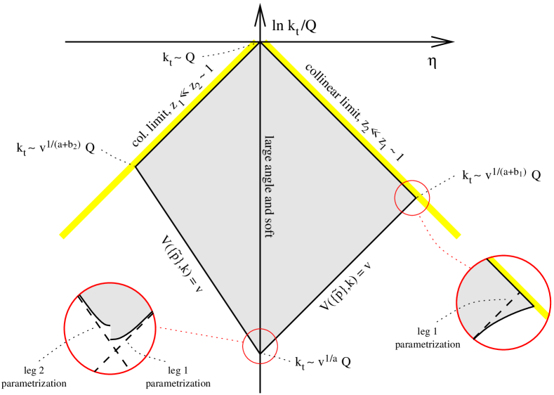
Figure 1: The $\eta$–$\ln(k_{t}/Q)$ plane for a single emission, together with a representation (shaded area) of the region in $k_{t}$ and $\eta$ over which the integrand of eq. (14b) is non zero. The specific positions of the lines correspond to the case of an observable with $a_{1}=a_{2}\equiv a=1$ and $b_{1}=1$, $b_{2}=3/2$. For simplicity, the $\phi$-dependence of the problem has been neglected. The insets correspond to a magnification by a factor of order $\ln 1/v$. Further details are given in the text.

To help us consider the issues that arise in the evaluation of eq. (14b), figure 1 shows in the $\eta$–$\ln(k_{t}/Q)$ plane, the region (shaded area) in which the integrand of eq. (14b) is non-zero, for some value of $v$. This region is delimited by two kinds of boundaries. Firstly, there are kinematic boundaries associated with the requirements $z^{(1)}<1$ and $z^{(2)}<1$. These give the upper edges of the shaded region. Secondly there are boundaries at $V(\{\tilde{p}\},k)=v$ associated with the $\Theta$-function in eq. (14b).

The intersections of the various boundaries set the characteristic scales (transverse momenta) of the problem. Firstly, the scale at the point where the two hard boundaries meet is of the order of the hard scale, $Q$, of the problem. In this corner, $z^{(1)}\sim z^{(2)}\sim 1$, eq. (13) is a poor approximation to the true real and virtual matrix elements. But the region $z^{(1)}\sim z^{(2)}\sim 1$ contributes at most at ${\cal{O}}\left(\alpha_{{\textsc{s}}}(Q)\right)$ (without logarithmic enhancements) to the integral, so the ‘error’ is NNLL and can accordingly be neglected.

Another scale arises, for each leg $\ell$, from the intersection between the kinematic boundary and the $\Theta$-function boundary, i.e. the left and right-hand corners of the shaded region. If one makes the assumption that one can extend the soft and collinear parametrisation (5) into the hard collinear region, then one finds, using eq. (10), that for a given fixed $z^{(\ell)}$, the observable scales as $k_{t}^{a_{\ell}+b_{\ell}}$. The scales associated with the lateral corners of the shaded region are then

$$k_{t}\sim v^{1/(a_{\ell}+b_{\ell})}Q\,.$$ (15)

In practice, in the hard collinear region, the observable $V(\{\tilde{p}\},k)$ may depart from its soft and collinear parametrisation (5). Such a situation is illustrated in the right-hand inset of fig. 1, which represents the true boundary of the shaded region (solid line), $V(\{\tilde{p}\},k)=v$, and the boundary that would be obtained based on the soft-collinear parametrised form for $V$ (dashed line). As long as the difference between the true form of the observable and the parametrisation is just a non-zero $z^{(\ell)}$-dependent factor of order $1$, then eq. (15) remains valid. Furthermore, when evaluating eq. (14b), replacing the true observable $V(\{\tilde{p}\},k)$ with its parametrised form leads to a difference of order $\alpha_{{\textsc{s}}}$, which is a NNLL correction.

From a practical (numerical) point of view, it is rather difficult to establish whether a departure from the parametrised form is of order $1$. However the condition can be formulated equivalently by requiring that for collinear emissions, almost everywhere, $V$ be non-zero and that

$$\left.\frac{\partial\ln V(\{\tilde{p}\},k)}{\partial\ln k_{t}^{(\ell)}}\right|_{\mathrm{fixed}\;z^{(\ell)},\,\phi^{(\ell)}}\!\!\!\!=\;\;a_{\ell}+b_{\ell}\,.$$ (16)

Here the expression ‘almost everywhere’ should be taken in its usual mathematical sense of everywhere except possibly a region of zero measure. An important point about eq. (16) concerns collinear safety: the observable must vanish as $k_{t}$ is taken to zero. Accordingly we have the condition $a_{\ell}+b_{\ell}>0$. A similar condition has been noted also in [22].

As a final source of characteristic scales of the problem, we have the intersection between the $\Theta$-function in eq. (14b) and the large-angle boundary between the hard legs. Let us temporarily assume that we can extend the soft and collinear parametrisation to the soft large-angle region. Then for leg $\ell$ the characteristic scale that emerges is

$$k_{t}\sim v^{1/a_{\ell}}Q\,.$$ (17)

We immediately see that a problem will arise if $a_{1}\neq a_{2}$: the knowledge that we have so far gathered about the observable does not tell us where, in $\eta$, the transition occurs between the parametrised forms for the different legs. This ambiguity corresponds to a single logarithmic integration from $k_{t}\sim v^{1/a_{1}}Q$ to $k_{t}\sim v^{1/a_{2}}Q$ over an unknown region of angle. Since the boundary between the legs may be determined by some potentially quite complex procedure, such as a jet algorithm, in a first instance it is preferable not to require any understanding of it.

One partial solution to this problem is to consider only observables for which $a_{1}=a_{2}$. This ensures that the ambiguity in the boundary between the two jets leads at most to an uncertainty in eq. (14b) of order $\alpha_{s}$ (NNLL). Fig. 1 illustrates this in the left-hand inset, in a case where additionally the true behaviour of the observable (solid lines) does not exactly follow the parameterisations (dashed lines). As long as this deviation from the parametrisation is by a factor of order $1$, in a limited region in angle, then it too will only affect eq. (14b) by a NNLL correction. Technically, it is most convenient to formulate the requirement as being that, for soft emissions, almost everywhere, $V$ should be non-zero and that

$$\left.\frac{\partial\ln V(\{\tilde{p}\},k)}{\partial\ln k_{t}^{(\ell)}}\right|_{\mathrm{fixed}\;\eta^{(\ell)},\,\phi^{(\ell)}}\!\!\!\!\equiv\;a\;=\;a_{1}\;=\;a_{2}\,.$$ (18)

This coincides with the condition for continuous globalness [12, 37], and ensures, at higher orders, the absence also of so-called non-global logarithms. Finally, we note that infrared safety implies $a>0$.

2.1.3 Evaluation of single-emission integrals

Given the extra requirements on the observable, eqs. (16) and (18), we are now in a position to carry out the integrations of eq. (14b), replacing $V(\{\tilde{p}\},k)$ with its parametrised form, eq. (5). As a shorthand, we introduce $R(v)$, (minus) the single-gluon contribution to $f$,

$$R(v)=\int[dk]|M^{2}(k)|\Theta(V(\{\tilde{p}\},k)-v)\,,$$ (19)

which can be written as

$$R(v)=\sum_{\ell=1}^{2}C_{F}\int^{Q^{2}}\frac{dk_{t}^{2}}{k_{t}^{2}}\int d\eta\,\frac{d\phi}{2\pi}\;\frac{\alpha_{{\textsc{s}}}(k_{t}^{2})}{2\pi}\;z^{(\ell)}p_{gq}(z^{(\ell)})\;\times\\ \;\times\Theta(\eta)\,\Theta(1-z^{(\ell)})\,\Theta\left(v-d_{\ell}\left(\frac{k_{t}}{Q}\right)^{a}e^{-b_{\ell}\eta^{(\ell)}}g_{\ell}(\phi)\right)\,.$$ (20)

We recall that the relations between $z^{(\ell)}$, $\eta$ and $\eta^{(\ell)}$ were given in section 2.1.1. Only one splitting function, $p_{gq}(z^{(\ell)})$, appears because the splitting function from the other leg has a very small argument and one can replace $zp_{gq}(z)=2$. The separation between the two legs has been arbitrarily placed at $\eta=0$.

We note the introduction of the scale $k_{t}^{2}$ for the coupling: though the scale of the coupling has no relevance at first order, it is useful to keep track of it in anticipation of what follows later.

For observables with $b_{\ell}\neq 0$, the $k_{t}$ integration in eq. (20) can be separated into two parts, according to whether the upper limit on $\eta$ stems from the $\Theta$-function of $1-z^{(\ell)}$, or from that associated with the observable. The boundary between the two regions occurs for $k_{t}\sim Qv^{\frac{1}{a+b_{\ell}}}$. We perform the $\eta$ integration separately in each of the two regions and write

$$R(v)=\sum_{\ell=1}^{2}C_{F}\left[\int^{Q^{2}}_{Q^{2}v^{\frac{2}{a+b_{\ell}}}}\frac{dk_{t}^{2}}{k_{t}^{2}}\;\frac{\alpha_{{\textsc{s}}}(k_{t}^{2})}{\pi}\left(\ln\frac{Q_{12}}{k_{t}}+B_{\ell}\right)+\right.\\ \left.+\int^{Q^{2}v^{\frac{2}{a+b_{\ell}}}}_{Q^{2}v^{\frac{2}{a}}}\frac{dk_{t}^{2}}{k_{t}^{2}}\,\frac{d\phi}{2\pi}\;\frac{\alpha_{{\textsc{s}}}(k_{t}^{2})}{\pi}\left(\ln\frac{Q_{12}}{2E_{\ell}}+\frac{1}{b_{\ell}}\ln\left[\left(\frac{k_{t}}{Q}\right)^{a}\frac{d_{\ell}g_{\ell}(\phi)}{v}\right]\right)\right]\,,$$ (21)

where we have neglected NNLL contributions associated with the exact position of the boundary between the two regions. In the upper $k_{t}$ region, the constant $B_{\ell}$ is associated with the large-$\eta$ part of the integration over the $p_{qg}$ splitting function,

$$B_{\ell}=\int_{0}^{1}\frac{dz}{z}\left(\frac{zp_{gq}(z)}{2}-1\right)=-\frac{3}{4}\,.$$ (22)

In the lower $k_{t}$ region, the upper limit on $\eta$ comes from the condition on the observable, and it is implicitly assumed that the observable (specifically, $d_{\ell}g_{\ell}(\phi)$) is positive definite.

It is convenient to express eq. (21) in terms of certain ‘standard building-blocks’,

$$R(v)=\sum_{\ell=1}^{2}C_{F}\left[r_{\ell}(L)+r_{\ell}^{\prime}(L)\left(\ln{\bar{d}}_{\ell}-b_{\ell}\ln\frac{2E_{\ell}}{Q}\right)+\right.\\ \left.+B_{\ell}\,T\!\left(\frac{L}{a+b_{\ell}}\right)\right]+2C_{F}\,T\!\left(\frac{L}{a}\right)\ln\frac{Q_{12}}{Q}\,,\qquad\quad L\equiv\ln\frac{1}{v}\,,$$ (23)

where

$$\ln{\bar{d}}_{\ell}=\ln d_{\ell}+\int_{0}^{2\pi}\frac{d\phi}{2\pi}\ln g_{\ell}(\phi)\,.$$ (24)

The ‘standard building blocks’ are the double logarithmic piece $r_{\ell}$ (containing all the LL and some NLL contributions),

$$r_{\ell}(L)=\int_{Q^{2}e^{-\frac{2L}{a+b_{\ell}}}}^{Q^{2}}\frac{dk_{t}^{2}}{k_{t}^{2}}\frac{\alpha_{{\textsc{s}}}(k_{t}^{2})}{\pi}\ln\frac{Q}{k_{t}}+\int_{Q^{2}e^{-\frac{2L}{a}}}^{Q^{2}e^{-\frac{2L}{a+b_{\ell}}}}\frac{dk_{t}^{2}}{k_{t}^{2}}\frac{\alpha_{{\textsc{s}}}(k_{t}^{2})}{\pi}\left(\frac{L}{b_{\ell}}+\ln\left(\frac{k_{t}}{Q}\right)^{a/b_{\ell}}\right),$$ (25)

as well as various purely single logarithmic (NLL) pieces,

$$T(L)=\int_{Q^{2}e^{-2L}}^{Q^{2}}\frac{dk_{t}^{2}}{k_{t}^{2}}\frac{\alpha_{{\textsc{s}}}(k_{t}^{2})}{\pi}\>,$$ (26)

and $r_{\ell}^{\prime}=\partial_{L}r_{\ell}$, which can be expressed in terms of the $T(L)$ as

$$r_{\ell}^{\prime}(L)=\frac{1}{b_{\ell}}\left[T\left(\frac{L}{a}\right)-T\left(\frac{L}{a+b_{\ell}}\right)\right]\,.$$ (27)

Though the results here have been derived for $b_{\ell}\neq 0$, their $b_{\ell}\to 0$ limit is finite and well-defined, as can straightforwardly be verified.

Several remarks are in order concerning eq. (23). Firstly, in the sum over legs, the contributions all depend just on $Q$ and the properties of the given leg — dependence on the invariant mass of the two legs, $Q_{12}$, has been placed outside the sum, and is independent of the $b_{\ell}$. Such a structure will be useful when extending the result to configurations with several hard legs.

Another point concerns frame dependence and $Q$ dependence of eq. (23). The derivation has been carried out in a specific Lorentz frame and with some arbitrary value for $Q$. The result should not however depend on the choice of frame or of $Q$. To see that it truly does not, we observe that a change of frame corresponds simply to a change in the values of the leg energies, $E_{\ell}\to E_{\ell}^{\prime}$. For a given emission this corresponds to change in rapidity with respect to the leg $\eta^{(\ell)}\to{\eta^{(\ell)}}^{\prime}$ and an associated change in the coefficients $d_{\ell}\to d_{\ell}^{\prime}$ (such that the observable remains frame-independent):

$${\eta^{(\ell)}}^{\prime} =\eta^{(\ell)}+\ln\frac{E_{\ell}^{\prime}}{E_{\ell}}\,,$$ (28a)

$$d_{\ell}^{\prime} =d_{\ell}+b_{\ell}\ln\frac{E_{\ell}^{\prime}}{E_{\ell}}\,.$$ (28b)

Inserting the change in $d_{\ell}$ into eq. (23), leads to the result that $R(v)$ is frame-independent.

The demonstration that eq. (23) is independent of the choice of $Q$ is only slightly more involved: at NLL accuracy, $r_{\ell}(v)$ depends on $Q$ as follows,

$$\frac{\partial r_{\ell}(L)}{\partial\ln Q}=T\left(\frac{L}{a}\right)-(a+b_{\ell})r_{\ell}^{\prime}+{\cal{O}}\left(\mathrm{NNLL}\right)\,,$$ (29)

while $T(L)$ and $r_{\ell}^{\prime}$ have $Q$ dependence only at NNLL accuracy. The $Q$-independence of the observable implies $\partial_{\ln Q}\ln d_{\ell}=a$. Inserting this into eq. (23), one finds that $R(v)$ is $Q$-dependent only at NNLL accuracy (strictly speaking, the NNLL terms arise only in the running-coupling case, so for the first-order, fixed-coupling result there is no $Q$-dependence at all).

2.2 All-order treatment ($\boldsymbol{q\bar{q}}$ case)

For the continuously global observables that we discuss in this article, the extension of the previous section’s treatment to all (NLL) orders involves two main ingredients: the running of the coupling, with its associated scheme dependence; and the treatment of multiple ‘independent’ emissions that are widely separated in rapidity.

This separation can be explained at second order for example by noting that in the soft and collinear region one can write the squared matrix element for two-gluon production as

$$|M^{2}(k_{1},k_{2})|=\left(|{M}^{2}(k_{1})||{M}^{2}(k_{2})|+|{\widetilde{M}}^{2}(k_{1},k_{2})|\right)\,,$$ (30)

where we have the product of two independent emissions, $|M^{2}(k)|$ being the squared matrix element for single gluon emission, as given in eq. (13), plus a correlated, ‘non-abelian’ part $|{\widetilde{M}}^{2}(k_{1},k_{2})|$ which contributes only when the two gluons are close in rapidity or both at large $z$ (there is also a corresponding part with a $q\bar{q}$ pair). This structure is a consequence of QCD coherence [53]: when two gluons are emitted on very different angular scales, the one at larger angle is emitted coherently from the combination of the quark and the gluon at smaller angle. Since the coherent combination of a quark and gluon has the same colour charge as a quark, the emission of two gluons on widely different angular scales simply behaves as independent emission. More generally, the emission of any number of gluons, all at very different angles, behaves as independent emission — this will be important for the all-order extension of eq. (30).

However, before dealing with the all-order generalisation of the independent emission part of eq. (30), we need first to consider the correlated part of the two-gluon emission, which is inextricably linked to the running of the coupling.

2.2.1 Correlated two-gluon emission

The treatment of the running coupling in resummations has been extensively discussed in the literature [1, 54, 55] and can be summarised essentially as follows. Firstly one considers the non-abelian (N.A.) correlated double emission term together with the non-abelian part of the virtual (1-loop) correction to single gluon emission, and notes that (including the $q\bar{q}$ contributions, without the $1/2!$)

$$[dk]\,|M^{2}_{\mathrm{1-loop,N.A.}}(k,\mu)|+\frac{1}{2!}\int[dk_{1}][dk_{2}]|{\widetilde{M}}^{2}(k_{1},k_{2})|\delta^{3}(k-k_{1}-k_{2})\\ =[dk]\,|M^{2}(k)|\left(\beta_{0}\ln\frac{k_{t}^{2}}{\mu^{2}}+\frac{K}{2\pi}\right)\alpha_{{\textsc{s}}}\,,$$ (31)

where the $\delta^{3}$-function is (in analogy to [56]) over the two components of the transverse momentum and the rapidity, and $\mu$ is the renormalisation scale; $\beta_{0}=(11C_{A}-2n_{\!f})/(12\pi)$ and, in the $\overline{\mbox{\scriptsize MS}}$ renormalisation scheme, $K=(\frac{67}{18}-\frac{\pi^{2}}{6})C_{A}-\frac{5}{9}n_{\!f}$. Thus one can add the $\alpha_{{\textsc{s}}}^{2}$ non-abelian terms to eq. (14b),

$$f(v)=1-\int[dk]\,\left(\,|M^{2}(k,\alpha_{{\textsc{s}}}\!=\!\alpha_{{\textsc{s}}}(\mu^{2}))|\,+|M^{2}_{\mathrm{1-loop,N.A.}}(k,\mu)|\right)\Theta(V(\{\tilde{p}\},k)-v)\\ -\frac{1}{2!}\int[dk_{1}][dk_{2}]|{\widetilde{M}}^{2}(k_{1},k_{2})|\Theta(V(\{\tilde{p}\},k_{1},k_{2})-v)\,,$$ (32)

and rewrite the result, using eq. (31), as

$$f(v)=1-\int[dk]\,|M^{2}(k,\alpha_{{\textsc{s}}}\!=\!\alpha_{{\textsc{s}}}(\mu^{2}))|\,\left(1+\left(\beta_{0}\ln\frac{k_{t}^{2}}{\mu^{2}}+\frac{K}{2\pi}\right)\alpha_{{\textsc{s}}}\right)\Theta(V(\{\tilde{p}\},k)-v)\\ -\frac{1}{2!}\int[dk_{1}][dk_{2}]|{\widetilde{M}}^{2}(k_{1},k_{2})|\left(\Theta(V(\{\tilde{p}\},k_{1},k_{2})-v)-\Theta(V(\{\tilde{p}\},k)-v)\right)\,,$$ (33)

where, in the second line, $k$ is a massless four-vector with the same transverse momentum and rapidity as $k_{1}+k_{2}$.

Reproducing the running coupling.

Let us initially just consider the first line of eq. (33). If one takes $\mu\sim Q$, then since $\ln k_{t}^{2}/Q^{2}$ is of the same order of magnitude as $\ln 1/v$, one sees that the $\beta_{0}$ term will correct the leading $\alpha_{{\textsc{s}}}(\mu^{2})\ln^{2}1/v$ contribution by an amount $\alpha_{{\textsc{s}}}^{2}\ln^{3}1/v$, also a LL contribution. The term involving $K$ leads to a correction of order $\alpha_{{\textsc{s}}}^{2}\ln^{2}1/v$, i.e. a NLL term. One can also choose to reabsorb these contributions into the leading term: taking $\mu=k_{t}$, the $\beta_{0}$ term disappears; furthermore defining $\alpha_{{\textsc{s}}}$ to be in the Bremsstrahlung (CMW) scheme [11, 54], $\alpha_{s,\mathrm{CMW}}=\alpha_{s,\overline{\mbox{\scriptsize MS}}}+K\alpha_{{\textsc{s}}}^{2}/2\pi$, one can reabsorb the term proportional to $K$.

It turns out that using $\alpha_{{\textsc{s}}}(k_{t}^{2})$ (as was anticipated in eq. (20)), in the CMW scheme, is sufficient to account for the running coupling contributions at all orders [2, 55], giving an implicit resummation of terms of the form $\beta_{0}^{n-1}\alpha_{{\textsc{s}}}^{n}\ln^{n+1}1/v$ and $K\beta_{0}^{n-2}\alpha_{{\textsc{s}}}^{n}\ln^{n}1/v$. The only proviso is that the running of $\alpha_{{\textsc{s}}}(k_{t})$ has to be carried out at two-loop level, in order to properly account also for NLL terms $\beta_{1}\beta_{0}^{n-3}\alpha_{{\textsc{s}}}^{n}\ln^{n}1/v$ ($n\geq 3$).

Strictly speaking this discussion applies to the region of soft and collinear gluon emission. Subtleties arise both in the hard-collinear and large-angle soft regions. In the former, the relation eq. (31) holds only at the accuracy of the $\beta_{0}$ term, but not of $K$. However since the hard-collinear region is single-logarithmic, the correction $K$ is associated with terms $\alpha_{{\textsc{s}}}^{n}\ln^{n-1}1/v$ and so is NNLL. For soft large-angle emissions, the problem is instead that there may be difficulties in identifying $k_{t}$: for the problems with two hard legs that we have discussed so far, one can show that it is the invariant transverse momentum with respect to the dipole that is the appropriate scale. However in ensembles with several hard legs (four or more), there is, to our knowledge, no procedure for unambiguously associating the emission with a particular dipole, and the appropriate definition of $k_{t}$ is ambiguous to within a factor of order $1$. Again, however, this ambiguity arises in a single-logarithmic region of integration over transverse momenta (at large angles) — writing such an integral as $\int^{Q}_{Av^{1/a}Q}\frac{dk_{t}}{k_{t}}\alpha_{{\textsc{s}}}(Bk_{t})$, where $A$ and $B$ are factors of order $1$ that parametrise our ignorance, and recalling that $\alpha_{{\textsc{s}}}(Bk_{t})\simeq\alpha_{{\textsc{s}}}(k_{t})+\beta_{0}\ln B\alpha_{{\textsc{s}}}^{2}(k_{t})/\pi$, it should be clear that the ambiguities translate to NNLL uncertainties proportional to $\ln A\alpha_{{\textsc{s}}}^{n}\ln^{n-1}1/v$ and $\ln B\alpha_{{\textsc{s}}}^{n}\ln^{n-1}1/v$.

Observable’s dependence on correlated gluon emission.

So far we have concentrated only on the first line of eq. (33), whose properties have been widely discussed in the literature. The second line, in contrast, has received less scrutiny, but nevertheless needs to be examined in some detail. Let us first consider the region where the relative transverse momentum of $k_{1}$ and $k_{2}$ (we label this $k_{t,12}$) is of the same order of magnitude as their transverse momenta with respect to the hard leg, $k_{t,12}\sim k_{t}$. This region of integration is suppressed by a power of $\alpha_{{\textsc{s}}}$ relative to the single-gluon emission. The question of how much it contributes to $f(v)$ depends on the observable: if $V(\{\tilde{p}\},k_{1},k_{2})$ differs from $V(\{\tilde{p}\},k)$ by no more than a factor of order $1$ then the difference of $\Theta$-functions in the second line of eq. (33) is non-zero only in a narrow band of $k$, where $V(\{\tilde{p}\},k)$ is of order $v$. Expressing this with reference to figure 1, one has a contribution of relative order $\alpha_{{\textsc{s}}}$ in a band of width $\sim 1$ (in $\ln k_{t}/Q$) along the lower edges of the shaded region. This corresponds to a NNLL term, $\alpha_{{\textsc{s}}}^{2}\ln 1/v$, which can be neglected. Such a contribution has been commented before in [17].

Suppose, instead, that the observable is such that $V(\{\tilde{p}\},k_{1},k_{2})$ differs substantially from $V(\{\tilde{p}\},k)$, say by a factor that grows as a power of $V(\{\tilde{p}\},k)$ — in this case the band in which the difference of $\Theta$-functions is non-zero will have a width of order $\ln 1/v$ and the second line of eq. (33) will contribute an amount $\alpha_{{\textsc{s}}}^{2}\ln^{2}1/v$, i.e. a NLL term. This would mean that the ‘correlated’ part of two-gluon emission could not simply be absorbed into the running of the coupling, necessitating a more sophisticated resummation treatment.

We also need to examine what happens where $k_{1}$ and $k_{2}$ are collinear and/or one of them is soft, $k_{t,12}\ll k_{t}$. At first sight it seems natural to argue that since we have an infrared and collinear (IRC) safe observable, $V(\{\tilde{p}\},k_{1},k_{2})\simeq V(\{\tilde{p}\},k)$ and so the difference of $\Theta$-functions is zero. This is certainly true in the limit $k_{t,12}/k_{t}\to 0$, but there is a question of how small the ratio $k_{t,12}/k_{t}$ has to be in order for the difference $|V(\{\tilde{p}\},k_{1},k_{2})-V(\{\tilde{p}\},k)|$ to be negligible (say less than $\varepsilon$). If the condition is for example $k_{t,12}/k_{t}\lesssim\varepsilon^{p}$ where $p$ is some arbitrary positive power, then one can show that the second line of eq. (33) will contribute at most an NNLL piece.

But if the condition instead involves $k_{t}/Q$, or $e^{-\eta}$ in the right-hand side, for example $k_{t,12}/k_{t}\lesssim\varepsilon^{p}(k_{t}/Q)^{p^{\prime}}$, then the difference of $\Theta$-functions will be non-zero over a large, logarithmic integration region in $k_{t,12}$ and the second line of eq. (33) could lead to contributions $\alpha_{{\textsc{s}}}^{2}\ln^{3}1/v$ or $\alpha_{{\textsc{s}}}^{2}\ln^{2}1/v$. In such a case, we would again be in a situation where the correlated two-gluon emission effects could not simply be absorbed into a pure running-coupling term.

Remarks.

It is quite often taken for granted that the effects of ‘correlated’ gluon emission can be absorbed into the running coupling in an appropriate scheme. The general analysis of this section reveals that this is true as long as the observable meets certain conditions — essentially that the scaling properties of the observable be the same whether there be one or two (or more) emissions; and that the IRC safety of the observable for secondary splitting of a primary emission should manifest itself for secondary splittings of the same order of magnitude of hardness as the primary emission.

The second of these conditions especially may seem quite non-intuitive. One is generally used to thinking of IRC safety in contexts where all the emissions (except the one being made collinear or soft) are of similar hardnesses, i.e. there is a single hard scale with respect to which one defines the degree of softness or collinearity. But when dealing with final-state resummations, one introduces a second scale in the problem, related to the (small) value of the observable. IRC safety merely states that the observable should be insensitive to an extra arbitrarily infrared or collinear emission — it does not specify at what scale that insensitivity should set in. It is natural to assume that it is simply the smaller of the two scales in the problem. If that is the case then the observable is resummable with ‘usual’ techniques. However there are observables for which the relevant ‘insensitivity scale’ involves some more complicated combination of the two scales in the problem, e.g. $k_{t}^{2}/Q$. A concrete example, which will be discussed in appendix F.3, is the Geneva $y_{23}$ jet-resolution parameter. Such observables require a more sophisticated resummation treatment, which is beyond the scope of this paper.

While the above discussion has been framed in terms of configurations with two correlated emissions, one should be aware that for the all-order reconstruction of the running coupling, the observable should have similar properties also with multiple correlated emissions and/or secondary collinear branchings. As we shall see, such a condition will actually turn out to form part of a more general class of requirements, which will be called recursive infrared and collinear (rIRC) safety.

2.2.2 Towards all orders

The picture that emerges from the above section is that, for suitable observables, two-gluon emission can be separated into two parts with distinct physical roles: there is a correlated part which provides scheme and running-coupling corrections to single-gluon emission; and there is an uncorrelated ‘independent-emission’ part, which we have yet to treat explicitly. There were two prerequisites for such a separation: firstly, we made use of a property of QCD matrix elements, QCD coherence [53], which guarantees that emissions widely separated in rapidity are effectively independent; secondly we specified a property of the observable, rIRC safety (to be further elaborated below), which guarantees, among other things, that the observable is sufficiently inclusive that the details of the correlations of emissions close in rapidity affect the predictions only at NNLL accuracy and beyond (except through the running of the coupling).

To generalise this to any number of emissions we make use of coherence at all orders: emissions at some given angular scale are emitted coherently from the ensemble of emissions at much smaller angles, meaning that emissions on disparate angular scales are effectively emitted independently. A priori however, there is no reason to believe that emissions are widely separated in rapidity — on the contrary it is straightforward to see that, for a typical event, any given region of rapidity of size $\Delta\eta\sim 1$ is likely to contain emissions.

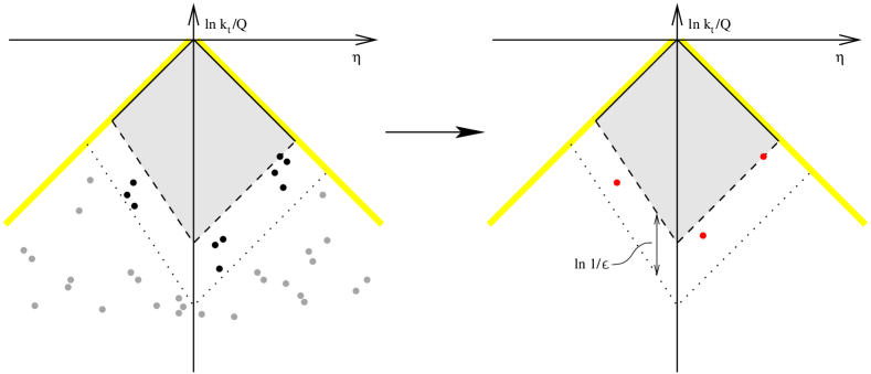
Figure 2: Illustrative pattern of emissions (dots) in the $\ln k_{t}$–$\eta$ plane (as in figure 1) given that the event shape has a value of order $v$ (corresponding to the dashed boundary). Left: emissions (grey) below the dotted line would each individually give a value of the observable $<\epsilon v$ and can be ignored (see text). Right: the remaining emissions (black) can be grouped into clusters local in rapidity, each cluster then being replaced by a single emission (red).

This is illustrated in the left-hand diagram of fig. 2, which shows a possible configuration of emissions (dots) that gives a value of order $v$ for the observable. To work around the problem of a ‘dense’ distribution of emissions in rapidity, we separate the emissions into two groups by introducing a small parameter $\epsilon$: emissions that individually would lead to a value of the observable smaller than $\epsilon v$ are coloured grey, and the remaining ones are coloured black. Most observables have the property (to be formalised below as part of the rIRC conditions) that the ‘grey’ emissions (dense in rapidity) can be removed from the ensemble without significantly altering the value of the observable. Therefore we are free to study configurations without these grey emissions.

As a next step we group the remaining ‘black’ emissions into clusters that are local in rapidity. The number of clusters per square of unit rapidity and $\ln 1/k_{t}$ is of order $\alpha_{{\textsc{s}}}$; given that the available rapidity is of order $\ln 1/v$ and that the range of $\ln 1/k_{t}$ over which the clusters are distributed (the height of the band between the dashed and dotted lines in figure 2) is $\ln 1/\epsilon$, the total number of clusters will be of order $\alpha_{{\textsc{s}}}\ln v^{-1}\ln\epsilon^{-1}$. By imposing $\alpha_{{\textsc{s}}}\ln 1/\epsilon\ll 1$, we can ensure that the total number of clusters is much smaller than the total available rapidity $\sim\ln v^{-1}$. Therefore when integrating over rapidities of emissions, the dominant contribution will come from configurations in which all clusters are widely separated in rapidity. Accordingly we can treat each cluster independently of the others.

We are then free, for each cluster, to proceed as we did with the correlated ${\widetilde{M}}^{2}(k_{1},k_{2})$ part of the two-gluon matrix element in section 2.2.1: for a cluster consisting of $m$ partons, $k_{i+1},\ldots,k_{i+m}$, we can replace $V(\{\tilde{p}\},\ldots,k_{i+1},\ldots,k_{i+m},\ldots)$ with $V(\{\tilde{p}\},\ldots,k_{i+1}+\ldots+k_{i+m},\ldots)$ and integrate inclusively over the momenta of the cluster partons, while keeping the total cluster momentum fixed. The fact that one can integrate inclusively over the parton momenta is guaranteed by continuous globalness together with the parts of the rIRC condition outlined in sec. 2.2.1 (and to which we return in detail in sections 2.2.4 and 3), and is critical in ensuring that one can make use of the standard result from resummation studies [1, 2, 54, 55, 59] that after additionally summing over $m$ one reproduces the all-order running coupling.

In the graphical representation of fig. 2, this last step corresponds to the replacement of the clusters of black emissions (left-hand diagram) with individual red emissions (right-hand diagram) with the same total momentum, as if each one were emitted independently with a coupling that runs as $\alpha_{{\textsc{s}}}(k_{t}^{2})$. It is this approximation of ‘independent emissions’ with running coupling (as well as a consistent treatment of virtual corrections, one that guarantees unitarity) that we will use in the next subsection, in order to calculate the all-order resummed distribution for our general observable.

First though, since we aim to guarantee NLL accuracy, it is important, in the above arguments, to review the accuracy of the approximations made in each step. The elimination of the ‘grey’ emissions (those individually giving a contribution $<\epsilon v$) leads to a correction suppressed by a positive power of $\epsilon$. In the limit of small $\alpha_{{\textsc{s}}}$, it is possible to make $\epsilon$ small, while maintaining $\alpha_{{\textsc{s}}}\ln\epsilon^{-1}\ll 1$, therefore this part of the procedure does not produce corrections to the logarithmic structure of the distribution.

A second potential source of inaccuracy might appear to come from the approximation that two clusters are independent even when they are close in rapidity. This problem can be avoided however, by making use of the freedom that we have in defining what is meant by a cluster: we recall that in section 2.2.1, we decomposed the two-gluon matrix element into two pieces. The two-correlated gluon piece, ${\widetilde{M}}^{2}(k_{1},k_{2})$ can be seen as a single-cluster term, while the independent emission piece, $M^{2}(k_{1})M^{2}(k_{2})$, acts as a two-cluster term. The combination of these two contributions reconstructs the full matrix element, the error made in treating the two gluons as independent (two-cluster piece) being compensated by the one-cluster piece. Similarly, in an $m$-gluon matrix element, as a consequence of coherence, it is possible to identify distinct contributions which behave as having one cluster (i.e. a contribution that is suppressed unless all partons are close in rapidity), two clusters (each local in rapidity, and independent of the other), and so on up to $m$ single-gluon ‘clusters’ (all independent). By basing our classification into clusters on such a decomposition of the matrix element (this is outlined in more detail in appendix D.1), and summing over all possible decompositions, one reproduces the full soft-collinear $m$-parton matrix element, without any approximations.

Therefore, the only source of logarithmic inaccuracy, in our approximation of independent emissions with running coupling, will come from our replacement (in the observable) of the individual momenta of the cluster partons by the total cluster momentum. We showed, in section 2.2.1, in the two gluon case, that for an rIRC safe observable this contributed at most $\alpha_{{\textsc{s}}}^{2}L$, i.e. a NNLL correction. Since, because of coherence, the details of gluon correlations inside a cluster are independent of the properties of all other clusters of emissions of the event, such a term will be independent of the contributions from other emissions (each one of which, with virtual corrections, may provide up to $\alpha_{{\textsc{s}}}L^{2}$), and one should immediately be able to see that in general the correction goes as $\alpha_{{\textsc{s}}}^{n}L^{2n-3}$.

In order to additionally meet the claims stated in section 1, i.e. to obtain a final form eq. (4), one should be able to show that, at all orders, corrections are at most of the form $\alpha_{{\textsc{s}}}h(\alpha_{{\textsc{s}}}L)e^{Lg_{1}(\alpha_{{\textsc{s}}}L)}$, where $h$ is some arbitrary function. To see why this is the case, one should first understand that the form eq. (4) has its origins in the exponentiated double-logarithmic Sudakov suppression associated with the resummation of the virtual corrections in the shaded region of fig. 2; factorised single-logarithmic corrections arise because of ${\cal{O}}\left(1\right)$ relative modifications to the observable’s value when there are multiple emissions in a narrow (single-logarithmic) strip along the boundary of the shaded region. A similar mechanism is relevant for the effects of non-inclusiveness of the observable with respect to the momenta of a cluster, except that by requiring two emissions to have the same rapidity (i.e. a cluster) one loses a logarithm, and a single-logarithmic factorised correction $\alpha_{{\textsc{s}}}^{n}L^{n}$ becomes a NNLL, $\alpha_{{\textsc{s}}}^{n}L^{n-1}$, factorised correction. A more mathematical treatment can only be given once we have seen in detail the origin, at single logarithmic level, of the structure of eq. (4). Accordingly it is deferred to appendix D.2 and for now we proceed with the independent-emission approximation, including running-coupling corrections.

2.2.3 Multiple independent emission

The result that we shall obtain here was first found in [21], however the derivation given here is intended to be slightly more direct and to highlight more fully the requirements that must be satisfied by the observable in order for the result to be valid.

For observables for whose resummation the picture of multiple independent emission is a good approximation (as discussed above), one can write at NLL accuracy

$$f(v)=\exp\left(-\int[dk]\,|M^{2}_{rc}(k)|\,\right)\sum_{n=0}^{\infty}\frac{1}{n!}\left(\prod_{i=1}^{n}\int[dk_{i}]\,|M^{2}_{rc}(k_{i})|\right)\times\\ \times\Theta(v-V(\{\tilde{p}\},k_{1},\ldots,k_{n}))\,,$$ (34)

where the first factor resums the virtual corrections, while the rest of the expression accounts for real emissions. Both real and virtual integrations should be understood as regularised. The coupling is always to be evaluated at scale $k_{t}$ and in the CMW scheme and the matrix element has been written with a subscript ‘$rc$’ as a reminder that running-coupling effects have already been resummed.

Note that in section 2.2.2, in order to guarantee the independent emission approximation, we removed all emissions below a softness and collinearity threshold, $\epsilon v$, those shown in grey in figure 2. Yet here, in our independent-emission formula, eq. (34), we have not imposed any such cut. This is legitimate because the condition that allowed us to remove these emissions (i.e. the fact they do not affect the value of the observable, a consequence of rIRC safety) also allows us to put them back in with some arbitrary distribution, in particular with an independent emission distribution.

An important point regarding eq. (34) concerns the manner in which one specifies the momenta $k_{i}$. In the case of a single emission we used the definition eq. (7), which has the property that the $k_{t}$ entering the definition coincides closely with the actual transverse momentum relative to the final Born partons (after recoil). This is important because the $dk_{t}^{2}/k_{t}^{2}dz/z$ divergence of the matrix element holds for a transverse momentum $k_{t}$ relative to the final Born momenta. When there are multiple emissions, the situation is more complicated: transverse momenta defined relative to fixed axes, as in eq. (7), do not necessarily coincide with the transverse momenta relative to the final Born partons. Since it is the latter that are of interest to us, when we refer to a given momentum $k_{i}$, it should be understood as being defined through its transverse momentum and rapidity (or energy fraction) relative to the final Born partons. In particular the actual 4-momentum components may well differ depending on what other emissions are present in the event. This point, and related issues, are discussed in more detail in appendix C.

To evaluate eq. (34), it will be convenient to identify the $k_{i}$ with the largest value of $V(\{\tilde{p}\},k_{i})$, and relabel it as $k_{1}$. We therefore rewrite the sum in eq. (34)

$$\sum_{n=0}^{\infty}\frac{1}{n!}\left(\prod_{i=1}^{n}\int[dk_{i}]\,|M^{2}_{rc}(k_{i})|\right)\\ =1+\int[dk_{1}]\,|M^{2}_{rc}(k_{1})|\,\sum_{m=0}^{\infty}\frac{1}{m!}\left(\prod_{i=2}^{m+1}\int[dk_{i}]\,|M^{2}_{rc}(k_{i})|\Theta(v_{1}-v_{i})\right)\,,$$ (35)

where we have introduced the notation $v_{i}\equiv V(\{\tilde{p}\},k_{i})$. The constant term, $1$, accounts for the case in which there are no emissions — because of the formally infinite suppression associated with the virtual corrections, it can from now on be neglected.

A technically useful step, next, as anticipated already in section 2.2.2, is to split the sum in eq. (35) into two parts, with emissions satisfying $v_{i}>\epsilon v_{1}$ and $v_{i}<\epsilon v_{1}$ respectively; $\epsilon$ is an arbitrary small parameter, which for suitable observables can be chosen such that $\epsilon\ll 1$, while $\ln 1/\epsilon\ll\ln 1/v$ (in the limit $v\to 0$ we assume that it is possible to choose $\epsilon$ independently of $v$). We thus write

$$\sum_{n=0}^{\infty}\frac{1}{n!}\left(\prod_{i=1}^{n}\int[dk_{i}]\,|M^{2}_{rc}(k_{i})|\right)=\\ \int[dk_{1}]\,|M^{2}_{rc}(k_{1})|\sum_{m=0}^{\infty}\frac{1}{m!}\left(\prod_{i=2}^{m+1}\int_{\epsilon v_{1}}^{v_{1}}[dk_{i}]\,|M^{2}_{rc}(k_{i})|\right)\times\\ \times\sum_{k=0}^{\infty}\frac{1}{k!}\left(\prod_{i=m+2}^{k+m+1}\int^{\epsilon v_{1}}[dk_{i}]\,|M^{2}_{rc}(k_{i})|\right),$$ (36)

where we have introduced the shorthand of integration limits that apply not directly to the $k_{i}$, but to the $v_{i}=V(\{\tilde{p}\},k_{i})$.

The above separation is of interest, because we require (as part of the rIRC safety conditions) that the emissions with $v_{i}<\epsilon v_{1}$ not contribute significantly to the final value of the observable, i.e.

$$V(\{\tilde{p}\},k_{1},\ldots,k_{m+1},k_{m+2},\ldots,k_{k+m+1})=V(\{\tilde{p}\},k_{1},\ldots,k_{m+1})+{\cal{O}}\left(\epsilon^{p}v_{1}\right)\,,$$ (37)

where $p$ is some positive power. So we can sum over these emissions without affecting the $\Theta$-function on the observable in eq. (34). This sum cancels the part of the virtual corrections associated with values of $k$ such that $V(\{\tilde{p}\},k)<\epsilon v_{1}$, allowing us to write

$$f(v)=\int[dk_{1}]\,|M^{2}_{rc}(k_{1})|\exp\left(-\int_{\epsilon v_{1}}[dk]\,|M^{2}_{rc}(k)|\,\right)\times\\ \times\sum_{m=0}^{\infty}\frac{1}{m!}\left(\prod_{i=2}^{m+1}\int_{\epsilon v_{1}}^{v_{1}}[dk_{i}]\,|M^{2}_{rc}(k_{i})|\right)\Theta(v-V(\{\tilde{p}\},k_{1},\ldots,k_{m+1}))\,.$$ (38)

We next take the virtual corrections and split them as follows

$$\exp\left(-\int_{\epsilon v_{1}}[dk]\,|M^{2}_{rc}(k)|\,\right)=e^{-R(\epsilon v_{1})}=e^{-R(v)-R^{\prime}\ln\frac{v}{\epsilon v_{1}}+{\cal{O}}\left(R^{\prime\prime}\right)}\,,\qquad\quad R^{\prime}\equiv\frac{dR}{d\ln 1/v}\,,$$ (39)

where $R(v)$ is the single-gluon contribution to $f(v)$, discussed in section 2.1.3, and we have expanded $R(\epsilon v_{1})$ around $v$, neglecting the second order ($R^{\prime\prime}=\partial^{2}_{\ln 1/v}R={\cal{O}}\left(\alpha_{{\textsc{s}}}^{n+1}L^{n}\right)$) term in the expansion, since it is NNLL (as long as eq. (38) is dominated by momenta $k_{1}$ such that $v_{1}\sim v$ — this is formalised in section 3.4). The resummed distribution can therefore be written

$$f(v)=e^{-R(v)}{\cal{F}}\,,$$ (40)

i.e. the exponential of the single gluon result, multiplied by a correction factor ${\cal{F}}$ which accounts for the details of the observable’s dependence on multiple emissions,

$${\cal{F}}=\int[dk_{1}]\,|M^{2}_{rc}(k_{1})|e^{-R^{\prime}\ln\frac{v}{\epsilon v_{1}}}\sum_{m=0}^{\infty}\frac{1}{m!}\left(\prod_{i=2}^{m+1}\int_{\epsilon v_{1}}^{v_{1}}[dk_{i}]\,|M^{2}_{rc}(k_{i})|\right)\times\\ \times\Theta(v-V(\{\tilde{p}\},k_{1},\ldots,k_{m+1}))\,.$$ (41)

The function ${\cal{F}}$ can be evaluated directly in this form, by Monte Carlo methods. However this tends not to be very efficient and it is worthwhile manipulating the expression a little further. This will be useful also to help us highlight the single-logarithmic nature of ${\cal{F}}$ and to eliminate subleading logarithmic contributions.

We introduce the notation $k^{(\rho)}$ for a momentum $k$ that has been subjected to a ‘generalised rescaling’ defined as follows: $V(\{\tilde{p}\},k^{(\rho)})=\rho\,V(\{\tilde{p}\},k)$; $\phi$ should not depend on the scaling; and the rapidity should scale as $\ln V(\{\tilde{p}\},k^{(\rho)})$, so that the whole of the phase-space remains covered after large rescalings. Figure 3 illustrates the effect of such a rescaling on three momenta represented in the $\eta$–$\ln(k_{t}/Q)$ plane (as introduced in fig. 1). An explicit form for the scaling can be obtained by introducing the maximum rapidity that an emission can have on leg $\ell$, for a given value of $v$,

$$\eta_{{\max},\ell}(v)=\frac{\ln 1/v}{a+b_{\ell}}+{\cal{O}}\left(1\right)\,,$$ (42)

(the piece of ${\cal{O}}\left(1\right)$ depends on the leg energy, and on $d_{\ell}g_{\ell}(\phi)$) and then parameterising an emission $k_{i}$’s rapidity as a fraction $\xi_{i}$ of this maximum rapidity, i.e. $\xi_{i}=\eta_{i}/\eta_{{\max},\ell}(V(\{\tilde{p}\},k_{i}))$. The rescaling is then fully specified by the requirement on the value of $V(\{\tilde{p}\},k_{i}^{(\rho)})$, the azimuthal angle and by the condition that $\xi_{i}$ be conserved,

$$k_{ti}^{(\rho)}=k_{ti}\,\rho^{(1-\xi_{i})/a+\xi_{i}/(a+b_{\ell})}\,,\qquad\eta_{i}^{(\rho)}=\eta_{i}-\frac{\xi_{i}\ln\rho}{a+b_{\ell}}\,,\qquad\phi_{i}^{(\rho)}=\phi_{i}\,.$$ (43)

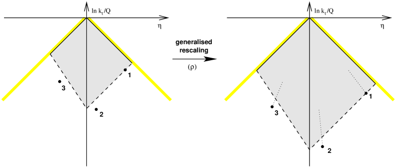
Figure 3: Left: three momenta in the $\eta$–$\ln(k_{t}/Q)$ plane. Right: those same three momenta after a common generalised rescaling $\rho$ has been applied to them; the dotted lines indicate the paths taken in the $\eta$–$\ln(k_{t}/Q)$ plane due to the rescaling. For each emission, the vertical distance to the dashed boundary is identical in the left and right-hand diagrams, consistent with a common scaling $\rho$ having been applied to all emissions.

Given this rescaling, we now need to introduce a new requirement on the observable, namely that when all momenta are scaled in the same fashion, the effect on the observable should be that same scaling:

$$V(\{\tilde{p}\},k_{1}^{(\rho)},\ldots,k_{m+1}^{(\rho)})=\rho\,V(\{\tilde{p}\},k_{1},\ldots,k_{m+1})\,.$$ (44)

This forms yet another part of the rIRC safety conditions. It may not be obvious why it should ever hold, nevertheless, it is satisfied for all commonly-studied event shapes. In the case of observables whose definitions involve just linear functions of the momenta, it can be understood as a direct consequence of this linearity.

The importance of eq. (44) is, in part, that it allows us to divide the integral over $k_{1}$ into an integral over the value of $v_{1}$ (or rather, over $\rho=v_{1}/v$) and an integral over the remaining degrees of freedom of $k_{1}$,

$${\cal{F}}=\int\frac{d\rho}{\rho}\int[dk_{1}]\,|M^{2}_{rc}(k_{1})|\,\delta\!\left(\ln\frac{v_{1}}{v}\right)e^{R^{\prime}\ln\rho\epsilon}\sum_{m=0}^{\infty}\frac{1}{m!}\left(\prod_{i=2}^{m+1}\int_{\epsilon v}^{v}[dk_{i}]\,|M^{2}_{rc}(k_{i})|\right)\times\\ \times\Theta(v-\rho V(\{\tilde{p}\},k_{1},\ldots,k_{m+1}))\,,$$ (45)

where a change of variables has been carried out, $k_{i}\to k_{i}^{(1/\rho)}$, giving $V(\{\tilde{p}\},k_{i})\to\rho V(\{\tilde{p}\},k_{i}^{(1/\rho)})$, and then the $k_{i}^{(1/\rho)}$ have been renamed $k_{i}$ so as to simplify the notation. We assume that the integral will be dominated by values of $\rho\sim 1$ (expressing the earlier assumption that $v_{1}\sim v$), which ensures that the neglected corrections to the $[dk_{i}]\,|M^{2}_{rc}(k_{i})|$ from the rescaling have at most a NNLL effect.

Thus one can integrate analytically over $\rho$ to obtain

$${\cal{F}}=\frac{e^{R^{\prime}\ln\epsilon}}{R^{\prime}}\int[dk_{1}]\,|M^{2}_{rc}(k_{1})|\,\delta\!\left(\ln\frac{v_{1}}{v}\right)\sum_{m=0}^{\infty}\frac{1}{m!}\left(\prod_{i=2}^{m+1}\int_{\epsilon v}^{v}[dk_{i}]\,|M^{2}_{rc}(k_{i})|\right)\times\\ \times\exp\left(-R^{\prime}\ln\frac{V(\{\tilde{p}\},k_{1},\ldots,k_{m+1})}{v}\right)\,.$$ (46)

This manipulation is of course valid only if the observable is positive definite.

That the resummation result can be expressed in terms of the product, eq. (40), of the exponential of the single-gluon result and the above function ${\cal{F}}$ was one of the main results of [21]. This separation is critical for our approach: all the double logarithmic terms are collected in the exponentiated single-gluon result and can be treated analytically, as was done in section 2.1. In contrast the function ${\cal{F}}$, which will usually have to be evaluated by Monte Carlo methods, is single-logarithmic. To see this let us rewrite $[dk_{i}]\,|M^{2}_{rc}(k_{i})|$ as follows:

$$\int[dk_{i}]\,|M^{2}_{rc}(k_{i})|=\sum_{\ell_{i}=1}^{2}\int\frac{dv_{i}}{v_{i}}\frac{C_{F}r^{\prime}_{\ell_{i}}}{{\cal N}_{\ell_{i}}(\alpha_{{\textsc{s}}}(Q)\ln v_{i})}\times\\ \times\int_{0}^{1}\frac{d\xi_{i}}{1+\frac{a+(1-\xi_{i})b_{\ell_{i}}}{a(a+b_{\ell_{i}})}2\beta_{0}\,\alpha_{{\textsc{s}}}(Q)\ln v_{i}}\int_{0}^{2\pi}\frac{d\phi_{i}}{2\pi}\,,$$ (47)

where we have taken into account the NLL correction due to the running of the coupling, $r^{\prime}_{\ell}$ is as defined in eq. (27), $\xi_{i}$ is the emission’s rapidity divided by the maximum possible rapidity for the given value of $v$, and ${\cal N}$ normalises the integral over $\xi_{i}$:

$$\xi_{i}=\frac{\eta_{i}}{\frac{1}{a+b_{\ell}}\ln\frac{1}{v_{i}}}\,,\quad\qquad{\cal N}_{\ell}(\alpha_{{\textsc{s}}}\ln v)=\int_{0}^{1}\frac{d\xi}{1+\frac{a+(1-\xi)b_{\ell}}{a(a+b_{\ell})}2\beta_{0}\,\alpha_{{\textsc{s}}}\ln v}\,.$$ (48)

In changing to an integral over the rapidity fraction $\xi_{i}$, and defining $\xi_{i}$ as in eq. (48) (where we have omitted contributions to the maximum rapidity of ${\cal{O}}\left(1\right)$), we have neglected various NNLL contributions associated with the exact upper and lower limits of the integrals. As a result, for a given value of $v_{i}$ the remaining part of the phase-space integrations and matrix element has the property that it depends only on the single-logarithmic quantity $\alpha_{{\textsc{s}}}(Q)\ln v_{i}$ (we recall that this is a property also of $r_{\ell_{i}}^{\prime}$).

Let us now take the $v\to 0$ limit of eq. (46) in such a way that $\beta_{0}\alpha_{{\textsc{s}}}\ln v\equiv\lambda$ is kept constant (and so also $r^{\prime}_{\ell}$). One obtains

$${\cal{F}}=\frac{e^{R^{\prime}\ln\epsilon}}{R^{\prime}}\sum_{m=0}^{\infty}\frac{1}{m!}\left(\prod_{i=1}^{m+1}\sum_{\ell_{i}=1}^{2}\int_{\epsilon}^{1}\frac{d\zeta_{i}}{\zeta_{i}}\frac{C_{F}r_{\ell_{i}}^{\prime}}{{\cal N}_{\ell_{i}}(\lambda/\beta_{0})}\int_{0}^{1}\frac{d\xi_{i}}{1+\frac{a+(1-\xi_{i})b_{\ell_{i}}}{a(a+b_{\ell})}2\lambda}\int_{0}^{2\pi}\frac{d\phi_{i}}{2\pi}\right)\times\\ \times\delta\!\left(\ln\zeta_{1}\right)\exp\left(-R^{\prime}\ln\lim_{v\to 0}\frac{V(\{\tilde{p}\},k_{1},\ldots,k_{m+1})}{v}\right),\qquad v_{i}\equiv\zeta_{i}v\,,$$ (49)

where we have neglected the difference between $\alpha_{{\textsc{s}}}\ln v_{i}$ and $\alpha_{{\textsc{s}}}\ln v$, and we emphasise that here the $k_{i}$ are functions of the $\xi_{i}$, $\phi_{i}$ and $v_{i}$, the limit $v\to 0$ being taken with $\xi_{i}$, $\phi_{i}$, and $\zeta_{i}=v_{i}/v$ constant. Since the generalised scaling that we discussed above, $k_{i}\to k^{(\rho)}_{i}$, is nothing but a scaling $v_{i}\to\rho v_{i}$ with $\xi_{i}$ and $\phi_{i}$ kept constant, eq. (44) ensures that the $v\to 0$ limit in eq. (49) is well defined. Strictly, eq. (44) would suggest that no $v\to 0$ limit is necessary. However there is a small fraction ($\sim 1/\ln\frac{1}{v}$) of configurations, with emissions close in rapidity (or at the extremities of the allowed rapidity region) that are allowed to violate eq. (44) and which contribute a NNLL correction to ${\cal{F}}$. Taking the $v\to 0$ limit ensures that they disappear, so that ${\cal{F}}$ is a purely single logarithmic function, free of any NNLL contamination.

There exist observables (typically those referred to as event shapes), for which a further simplification of eq. (49) is possible. They have the property that for small $v_{i}$ the observable is independent of the $\xi_{i}$ values (except potentially, non-asymptotically, for $\xi_{i}$ close to $0$ or $1$). Accordingly one can perform the $\xi_{i}$ integrations analytically and write

$${\cal{F}}=\frac{e^{R^{\prime}\ln\epsilon}}{R^{\prime}}\sum_{m=0}^{\infty}\frac{1}{m!}\left(\prod_{i=1}^{m+1}\sum_{\ell_{i}=1}^{2}C_{F}r_{\ell_{i}}^{\prime}\int_{\epsilon}^{1}\frac{d\zeta_{i}}{\zeta_{i}}\int_{0}^{2\pi}\frac{d\phi_{i}}{2\pi}\right)\delta\!\left(\ln\zeta_{1}\right)\times\\ \times\exp\left(-R^{\prime}\ln\lim_{v\to 0}\frac{V(\{\tilde{p}\},k_{1},\ldots,k_{m+1})}{v}\right),\qquad v_{i}\equiv\zeta_{i}v\,,\qquad\xi_{i}=\mathrm{any}\,,$$ (50)

where one is free in one’s choice of the $\xi_{i}$ values to be used for fixing the $k_{i}$. Typically one takes $\xi_{i}$ far from the edges of rapidity, which nearly always ensures that any finite-$v$ corrections disappear rapidly, e.g. as a power of $v$, rather than as a power of $1/\ln\frac{1}{v}$ as is the case for eq. (49).

2.2.4 Recursive IRC safety

In the above derivation, we have made repeated use of properties of the observable which we referred to as being elements of a novel condition called recursive IRC safety. Let us now assemble those elements.

When discussing two-correlated-parton emission, section 2.2.1, we introduced the requirement that for two soft and/or collinear partons of similar hardness and close in rapidity, the observable should have a value of the same order of magnitude as in the presence of just one of those partons. As discussed in section 2.1.2, it is difficult in numerical codes to unambiguously check the requirement that two values be of the same order of magnitude. It is instead simpler (and equivalent) to check that they have the same scaling as one varies an overall softness scale. A similar requirement, i.e. that the observable scale in the same fashion with multiple emissions as with a single emission, also appeared in the context of our treatment of multiple independent emission in section 2.2.3. Both of these requirements can actually be expressed in terms of a single condition, as follows.

We define a momentum function $\kappa_{i}(\zeta)$ such that $V(\kappa_{i}(\zeta),\{\tilde{p}\})=\zeta$, in analogy with the rescalable momentum $k_{t}^{(\rho)}$ of eq. (43), but generalised so that it is now specified by three parameters, $\eta^{0}_{i}$, $\xi_{i}$, and $\phi_{i}$, as well as the leg index $\ell_{i}$,

$$\eta_{i}(\zeta)=\eta^{0}_{i}-\frac{\xi_{i}\ln\zeta}{a+b_{\ell_{i}}}\,,\qquad\quad\kappa_{ti}(\zeta)=\left(\frac{\zeta e^{b_{\ell_{i}}\eta_{i}(\zeta)}}{d_{\ell_{i}}g_{\ell_{i}}(\phi_{i})}\right)^{\frac{1}{a}},\qquad\quad\phi_{i}(\zeta)\equiv\phi_{i}\,,$$ (51)

corresponding to a linear path in the $\eta$–$\ln k_{t}$ plane. Asymptotically ($\zeta\to 0$), any other functional form will either be nonsensical (e.g. outside the allowed phase-space) or else approximate a linear path. Not all values are allowed for the parameters, in particular $0\leq\xi_{i}\leq 1$ and for certain values of the $\eta^{0}_{i}$ the emission may be kinematically allowed only for sufficiently small $\zeta$ (or disallowed altogether if $\xi_{i}=1$).

We then require that for any $m$ such momentum functions, independently of the $\xi_{i}$, $\eta^{0}_{i}$ and $\phi_{i}$ ($i=1\ldots m$), the following limit,

$$\lim_{{\bar{v}}\to 0}\frac{1}{{\bar{v}}}V(\{\tilde{p}\},\kappa_{1}({\bar{v}}\zeta_{1}),\ldots,\kappa_{m}({\bar{v}}\zeta_{m}))\,,$$ (52)

be well-defined and non-zero, for any choice of (non-zero) values of the $\zeta_{i}$. We introduce here $\bar{v}$, a parameter that we are free to vary to probe the observable’s properties, and distinguish it from $v$ which, from now on, will just denote the particular value of the observable for which we resum the distribution.

The above condition guarantees that in the limit of small $\bar{v}$, any set of emissions close to the boundary $V(\{\tilde{p}\},k)=\bar{v}$ will lead to a value for the observable of order $\bar{v}$ (because otherwise, there will exist choices of $\kappa_{i}(\zeta)$ and $\zeta_{i}$ such that the limit is infinite, zero, or ill-defined).

By defining some of the $\kappa_{i}$ in eq. (52) such that they have identical $\xi_{i}$, one obtains a set of momenta that stay close in rapidity as the emissions are scaled towards the soft-collinear limit, precisely like the correlated emissions of section 2.2.1, thus embodying the rIRC safety condition discussed in the first paragraph of the part of section 2.2.1 labelled ‘Observable’s dependence on correlated gluon emission’. Taking different $\xi_{i}$ values for the various emissions, the part of rIRC safety expressed in eq. (44) is also embodied, since we are free to fix the $\eta^{0}_{i}$ so as to reproduce eq. (43).

Eq. (52) lays the basis for the next part of the rIRC safety condition, that which actually resembles plain IRC safety. For plain IRC safety, given some ensemble of partons, one requires that the additional soft and/or collinear splitting of one (or more) of those partons not change the value of the observable by more than a positive power of the softness/collinearity of the splitting(s), normalised to the hard scale $Q$.

In the context of resummations we effectively have two relevant scales: $Q$ and the scale (as a function of rapidity) set by the boundary $V(\{\tilde{p}\},k)=v$. To be able to carry out the resummation, in addition to IRC safety, we needed to assume (see sections 2.2.2, 2.2.3) that, for sufficiently small $v$, there exists some $\epsilon\ll 1$, that can be chosen independently of $v$, such that we can neglect any splitting that is at a smaller scale than that defined by $\epsilon v$ (to within an absolute correction to $V$ of order $\epsilon^{p}v$, with $p$ some positive power). The crucial extension compared to plain IRC safety is in the fact that one should be able to choose $\epsilon$ independently of $v$.

In terms of the momentum functions $\kappa_{i}(\zeta)$, textbook statements of IRC safety can be expressed with requirements such as

$$\lim_{\zeta_{m+1}\to 0}V(\{\tilde{p}\},\kappa_{1}({\bar{v}}\zeta_{1}),\ldots,\kappa_{m}({\bar{v}}\zeta_{m}),\kappa_{m+1}({\bar{v}}\zeta_{m+1}))\\ =V(\{\tilde{p}\},\kappa_{1}({\bar{v}}\zeta_{1}),\ldots,\kappa_{m}({\bar{v}}\zeta_{m}))\,.$$ (53)

The equivalent statement for rIRC safety exploits the scaling property of the observable, i.e. the fact that eq. (52) is well-defined and finite, to then define a double limit,

$$\lim_{\zeta_{m+1}\to 0}\lim_{{\bar{v}}\to 0}\frac{1}{{\bar{v}}}V(\{\tilde{p}\},\kappa_{1}({\bar{v}}\zeta_{1}),\ldots,\kappa_{m}({\bar{v}}\zeta_{m}),\kappa_{m+1}({\bar{v}}\zeta_{m+1}))\\ =\lim_{{\bar{v}}\to 0}\frac{1}{{\bar{v}}}V(\{\tilde{p}\},\kappa_{1}({\bar{v}}\zeta_{1}),\ldots,\kappa_{m}({\bar{v}}\zeta_{m}))\,.$$ (54)

The order of the limits on the left-hand-side is crucial: if the softness/collinearity $\zeta_{m+1}$ at which the $(m+1)^{\mathrm{th}}$ emission becomes irrelevant depends on $\bar{v}$ (e.g. it scales as a power of $\bar{v}$), then for infinitely small $\bar{v}$ the $(m+1)^{\mathrm{th}}$ emission will never become irrelevant and the equality will not be satisfied. One can also combine eqs. (53) and (54) to obtain an alternative statement of the rIRC safety condition in terms of the commutator of the limits:

$$\left[\lim_{\zeta_{m+1}\to 0},\lim_{{\bar{v}}\to 0}\right]\ \frac{1}{{\bar{v}}}V(\{\tilde{p}\},\kappa_{1}({\bar{v}}\zeta_{1}),\ldots,\kappa_{m}({\bar{v}}\zeta_{m}),\kappa_{m+1}({\bar{v}}\zeta_{m+1}))=0\,.$$ (55)

In addition to the limit where an extra emission is made soft/collinear to the hard leg (relevant in sections 2.2.2 and 2.2.3), we also need to consider the situation where one or more existing emissions split softly and/or collinearly (as discussed in sections 2.2.1 and 2.2.2). We represent the collinear splitting of an existing emission with the notation $\kappa_{i}(\zeta)\to\{\kappa_{i_{a}},\kappa_{i_{b}}\}(\zeta,\mu)$, such that $\mu^{2}=(\kappa_{i_{a}}+\kappa_{i_{b}})^{2}/\kappa_{ti}^{2}$ and $\lim_{\mu\to 0}\left(\kappa_{i_{a}}+\kappa_{i_{b}}\right)=\kappa_{i}$. We then for example require

$$\lim_{\mu\to 0}\lim_{{\bar{v}}\to 0}\frac{1}{{\bar{v}}}V(\{\tilde{p}\},\kappa_{1}({\bar{v}}\zeta_{1}),\ldots,\{\kappa_{i_{a}},\kappa_{i_{b}}\}({\bar{v}}\zeta_{i},\mu),\ldots\kappa_{m}({\bar{v}}\zeta_{m}))\\ =\lim_{{\bar{v}}\to 0}\frac{1}{{\bar{v}}}V(\{\tilde{p}\},\kappa_{1}({\bar{v}}\zeta_{1}),\ldots,\kappa_{i}({\bar{v}}\zeta_{i}),\ldots,\kappa_{m}({\bar{v}}\zeta_{m}))\,,$$ (56)

regardless of how the $\mu\to 0$ limit is taken — i.e. whether at fixed relative energy fractions for $\kappa_{i_{a}}$, $\kappa_{i_{b}}$ or with one of them simultaneously becoming softer than the other. Making use of plain IRC safety, eq. (56) too can can be expressed in terms of a commutator of limits, as in eq. (55).

Eqs. (54) and (56), together with the condition that (52) be well defined, summarise the requirements that make up rIRC safety. Combined with the form eq. (5) for the observable in the soft and collinear limit, and the continuous globalness condition, rIRC safety ensures the validity, to NLL accuracy, of the approximations that we have made in order to arrive at eq. (40) together with eqs. (23) and (49).

It is quite deliberately that we stated that eqs. (54) and (56) ‘summarise’ rIRC safety. Indeed, as discussed in appendix G, widespread mathematical statements of normal IRC safety, such as eq. (53), are also merely summaries of full IRC safety, for which we are not aware of a complete mathematical formulation. Thus for IRC safety it is in some respects more accurate to state it in words, i.e. that an observable should be insensitive to soft and/or collinear branchings. Similarly, part 2 of rIRC safety is more fully described by the paragraph preceding eq. (53) than by eqs. (54) and (56), and, for example, exceptions to eq. (52) are allowed, as long as they correspond to sets of configurations having zero measure in the space $\prod_{i}(d\zeta_{i}d\eta^{0}_{i}d\phi_{i})$.

A more general question arises as to whether rIRC safety and continuous globalness, are the necessary and sufficient conditions for the form eq. (4) to be correct. Since eq. (40) is a specific case of eq. (4), these conditions should certainly be sufficient. However they are not necessary — we know for example of non-global observables that have a resummed distribution of the form eq. (4) [12, 37]. Furthermore, we believe that there exist observables that fail a subset of the rIRC conditions, but which nevertheless also have a resummed distribution with the structure eq. (4) — we suspect the Geneva jet resolution threshold, discussed in appendix F.3, of being an example of such an observable.

The specificity of observables that fail some of our applicability conditions, but at the same time have a resummed structure as in eq. (4) is, we suspect, that they cannot be resummed by just the double logarithmic resummation of virtual contributions with corrections coming exclusively from dynamics at the scale of the lower boundary of the excluded region. A deeper understanding of this point would, however, require further investigation.

2.3 Generalisation to other Born configurations

The discussion till now has been limited to the case of a Born configuration consisting of a single outgoing hard quark-antiquark pair. Much of it carries over relatively straightforwardly to more general cases — in particular all the applicability conditions that we have discussed are simply related to the general classes of divergence that are found in multi-parton matrix elements (soft and collinear divergences with respect to the Born partons and also with respect to any further emitted partons). No new classes of divergence appear when going beyond the simple 2-outgoing jet case studied above, and therefore the applicability conditions will remain valid quite generally.

The main non-trivial modifications relative to the results of section 2.2 concern the structure of single-logarithmic contributions associated with incoming legs (collinear single-logarithms) and with the colour structure of configurations with more than two legs (soft large-angle single-logarithms), both of which issues have been extensively discussed in the literature.

2.3.1 Incoming hard legs

Implicit in our discussion so far is that the probability $f(v)$ multiplies the hard cross section for the underlying Born event, cf. eq. (3). In processes with incoming legs, that hard cross section is evaluated using a procedure which factorises collinear divergences along each incoming leg into an associated parton density function, $q(x,\mu_{F}^{2})$. One generally chooses a factorisation scale $\mu_{F}$ of the order of the hard scale $Q$.

The factorisation procedure for the Born cross section involves an integration over collinear emissions with transverse momenta up to scale $\mu_{F}$, which ‘builds up’ the parton density function at scale $\mu_{F}$. However, when one places a limit $v$ on the value of the final-state observable, one vetoes collinear emissions with $(k_{t}/Q)^{a+b_{\ell}}\gtrsim v$. Due to rIRC safety, the remaining hard collinear emissions (those at lower values of $k_{t}$) do not affect the value of the observable, and can be therefore integrated over to ‘build up’ the parton density to a scale of the order of $Qv^{1/(a+b_{\ell})}$. The probability $f(v)$ therefore includes a correction factor

$$\frac{q(x,\mu_{F}^{2}v^{2/(a+b_{\ell})})}{q(x,\mu_{F}^{2})}\,,$$ (57)

so that the parton density $q(x,\mu_{F}^{2})$ that was included in the Born cross section is effectively replaced with a parton density at the new, lower factorisation scale (the choice of $Qv^{1/(a+b_{\ell})}$ or $\mu_{F}v^{1/(a+b_{\ell})}$ being of course arbitrary, since they differ only by NNLL corrections). We note that above the scale $\mu_{F}v^{1/(a+b_{\ell})}$ there remains the virtual part of the collinear corrections, already accounted for by the $B_{\ell}$ term in eq. (23).

The above result is simply a generalisation of the one for the widely studied Drell-Yan transverse momentum resummation [1, 54, 59], and has also been quite extensively discussed for event shapes [23, 26, 27, 28]. Nevertheless, in Appendix E we revisit the derivation of eq. (57), giving special emphasise to the requirement of rIRC safety.

2.3.2 Three hard legs

NLL final-state resummations for Born events consisting of a hard quark-(anti)quark pair and a hard gluon have been discussed in [25, 26, 27, 28]. The treatment of a general observable in the 3-jet case mirrors quite closely that given above for 2 jets. The main difference is that $R(v)$ originates from a sum over three dipoles, as opposed to a single dipole: a $qq^{\prime}$ dipole ($q$ and $q^{\prime}$ being respectively the quark and (anti)quark) which is associated with a colour factor $(C_{F}-C_{A}/2)$, and the $qg$ and $q^{\prime}g$ dipoles ($g$ being the gluon) each associated with the colour factor $C_{A}/2$.

Schematically one can therefore write $R$ as

$$R(v)=\sum_{\mathrm{dipoles}}C_{\mathrm{dipole}}\left(\sum_{\ell\in\mathrm{dipole}}\left[r_{\ell}(L)+r_{\ell}^{\prime}(L)\left(\ln{\bar{d}}_{\ell}-b_{\ell}\ln\frac{2E_{\ell}}{Q}\right)+\right.\right.\\ \left.\left.+B_{\ell}\,T\!\left(\frac{L}{a+b_{\ell}}\right)\right]+2\,T\!\left(\frac{L}{a}\right)\ln\frac{Q_{\mathrm{dipole}}}{Q}\right),$$ (58)

where $C_{\mathrm{dipole}}$ is the colour factor associated with the dipole. Note that for the gluonic leg, $B_{\ell}$ has a different value than in the quark case. It can be determined from the collinear matrix elements for $g\to gg$ and $g\to q\bar{q}$ splitting,

$$|M^{2}_{\ell,g\to gg}(k)| =\frac{\alpha_{{\textsc{s}}}C_{A}}{2\pi}\,\frac{z^{(\ell)}p_{gg}(z^{(\ell)})}{k_{t}^{2}}\,,\qquad p_{gg}(z)=\frac{2(1-z)}{z}+z(1-z)\,,$$ (59a)

$$|M^{2}_{\ell,g\to q\bar{q}}(k)| =\frac{\alpha_{{\textsc{s}}}T_{R}}{2\pi}\,\frac{z^{(\ell)}p_{qg}(z^{(\ell)})}{k_{t}^{2}}\,,\qquad p_{qg}(z)=z^{2}+(1-z)^{2}\,,$$ (59b)

where we have exploited the $z\leftrightarrow 1-z$ symmetry of the $g\to gg$ splitting to write $p_{gg}$ such that it only has a $z\to 0$ divergence (cf. eq. (5.41) of [52]). The gluonic $B_{\ell}$ value is then given by

$$B_{\ell}^{(\mathrm{gluon})}=\int_{0}^{1}\frac{dz}{z}\left(\frac{zp_{gg}(z)}{2}+\frac{T_{R}n_{\!f}\,zp_{qg}(z)}{2C_{A}}-1\right)=\frac{-11C_{A}+4T_{R}n_{\!f}}{12C_{A}}\,,$$ (60)

where, as in eq. (22), we extract the overall colour factor associated with the soft divergence, which will reappear below, after explicitly summing over dipoles.

The presence of sums over dipoles and over their associated legs in eq. (58) is somewhat cumbersome (as well as difficult to generalise subsequently). However we can invert the order of the sums over legs and dipoles, and perform the sum over dipoles to obtain

$$R(v)=\sum_{\ell=1}^{n}C_{\ell}\left[r_{\ell}(L)+r_{\ell}^{\prime}(L)\left(\ln{\bar{d}}_{\ell}-b_{\ell}\ln\frac{2E_{\ell}}{Q}\right)+B_{\ell}\,T\!\left(\frac{L}{a+b_{\ell}}\right)\right]\\ -\ln S\left(T\left(\frac{L}{a}\right)\right),$$ (61)

where $n=3$ is the number of legs, and we have exploited the fact that for each leg, $\sum_{\mathrm{dipole}\supset\{\ell\}}C_{\mathrm{dipole}}=C_{\ell}$, with $C_{\ell}$ the colour factor of the given leg, $C_{F}$ for the (anti)quarks and $C_{A}$ for the gluon. The function $S$ collects the terms that cannot be conveniently expressed as a sum over individual legs,

$$\ln S(t)=-t\left[{C_{A}}\ln\frac{Q_{qg}Q_{q^{\prime}g}}{Q_{qq^{\prime}}Q}+2C_{F}\ln\frac{Q_{qq^{\prime}}}{Q}\right]\,.$$ (62)

One can verify that the $Q$ dependence of $\ln S(t)$ is reducible to the form $t\,C_{T}\ln Q$, with $C_{T}=\sum_{\ell}C_{\ell}$, as is necessary for $R(v)$ overall to be $Q$-independent. The remaining part of $S$ accounts for the coherent structure of large-angle radiation from the ensemble of hard legs.

Eq. (61) is of course only the single-gluon result. The full all-order result needs to be obtained by following a procedure analogous to that given in section 2.2. As was shown in [25] the decomposition into a structure of three dipoles holds at all orders, which means that the analysis carries through essentially unchanged, the only difference being that, for ${\cal{F}}$, the sum over two legs in eqs. (47)–(50) should be generalised to a sum over three legs and $C_{F}$ should be replaced with the appropriate leg colour factor.

We finally note that processes such as $gg\to\mathrm{Higgs}+g$, which involve three gluonic legs, or equivalently three gluon-gluon dipoles, can be treated in a similar manner, the only difference being that each dipole is associated with a colour factor $C_{A}/2$, so that in eq. (62) one needs to replace $C_{F}$ with $C_{A}$.

2.3.3 Four hard legs and beyond

A crucial property of the two and three-jet cases is that there is a unique structure of colour flow for the underlying hard process — a single dipole in the two-jet case, and a sum over (the $3$) dipoles made from all pairs of hard legs in the $3$-jet case. This means that a loop virtual correction does not change the colour structure of the underlying hard event, and it is this property that allows us to straightforwardly exponentiate the single-gluon term, $\int[dk]\,|M^{2}_{rc}(k)|$, in the virtual corrections in eq. (34).

In processes with four or more hard jets the situation is more complex, as was discussed originally in [39, 40, 41, 42, 43]. To illustrate the point concretely, let us consider the process $q\bar{q}\to q\bar{q}$, where for example the incoming $q\bar{q}$ pair can form a colour singlet or a colour octet. Both the hard matrix element and the pattern of large-angle soft radiation (and associated virtual corrections) depend on the overall colour of the incoming pair. Additionally a loop correction (stretched say across the incoming and outgoing quarks) can modify the overall colour of the $q\bar{q}$ pair entering the hard scattering: loop corrections introduce mixing between the different colour structures, and at all orders one needs to resum the resulting mixing matrix.

As explained in detail in [41], one needs to keep track separately of the colour channel of the Born amplitude and its complex conjugate. Denoting the possible colour channels by an index $I$, one has (in the notation of the above papers) a matrix $H_{II^{\prime}}$ for the product of the Born amplitude and its complex conjugate, respectively in colour channels $I$, $I^{\prime}$, modulo the normalisation associated with the colour algebra, contained in a matrix $M_{II^{\prime}}$ (which, for the orthogonal, but non-normal choice of colour basis in [41, 42] is a diagonal matrix). The differential Born cross section (modulo an overall kinematic normalisation) is given by $\mathop{\mathrm{Tr}}(HM)\equiv H_{II^{\prime}}M_{I^{\prime}I}$.

In the two and three-jet cases we had been able to write the (double-logarithmic) virtual corrections as the exponential of an integral over the single-gluon matrix element, $\exp\left(-R(v)\right)=\exp\left(-\int_{v}[dk]|M^{2}_{rc}(k)|\right)$. As already indicated, in the multi-jet case, the virtual corrections are now matrices in colour space, which act separately on the amplitude and its complex conjugate. Given the form of these matrices as presented in [39, 40, 41, 42, 43] (specifically for $2\to 2$ scattering) and [3] (in generic form), $\exp\left(-R(v)\right)$ can be written

$$e^{-R(v)}\equiv\frac{(e^{-\frac{1}{2}\int_{v}[dk]\gamma(k)-\frac{i}{2}CT\left(\frac{L}{a}\right)})_{JI}(e^{-\frac{1}{2}\int_{v}[dk]\gamma(k)+\frac{i}{2}CT\left(\frac{L}{a}\right)})_{J^{\prime}I^{\prime}}H_{II^{\prime}}M_{J^{\prime}J}}{\mathop{\mathrm{Tr}}(HM)}=\\ =\frac{\mathop{\mathrm{Tr}}\left(e^{-\frac{1}{2}\int_{v}[dk]\gamma(k)-\frac{i}{2}CT\left(\frac{L}{a}\right)}He^{-\frac{1}{2}\int_{v}[dk]\gamma^{\dagger}(k)+\frac{i}{2}C^{\dagger}T\left(\frac{L}{a}\right)}M\right)}{\mathop{\mathrm{Tr}}(HM)}\,.$$ (63)

where both $\gamma_{JI}(k)$ and $C_{JI}$ are real matrices. Each entry of $\gamma_{JI}(k)$ can be written as a linear combination of dipole emission matrix elements. Furthermore in the limit of $k$ being collinear to a hard leg $\ell$, $\gamma_{JI}(k)=|M^{2}_{\ell,rc}(k)|(\delta_{JI}+{\cal{O}}\left(\smash{e^{-\eta^{(\ell)}}}\right))$, where $|M^{2}_{\ell,rc}(k)|$ is the matrix element for emission collinear to leg $\ell$, eq. (11), with the addition of a running coupling — this reduction, in the collinear limit, of $\gamma_{JI}(k)$ to $|M^{2}_{\ell,rc}(k)|\delta_{JI}$ is a manifestation of coherence, i.e. the independence of the dynamics at small angular scales from that at large angular scales. In the cases studied so far (and we believe more generally), the entries of the $C_{JI}$ matrix are simply combinations of colour factors (i.e. without any dependence on the Born kinematics), whose structure is closely related to that of the $\gamma_{JI}(k)$. They give rise to the non-cancelling parts of Coulomb phases. One notes that $C_{JI}$ is multiplied by $T\left(\frac{L}{a}\right)$, a signal of its large-angle origin — quite generally, it is only the (single-logarithmic) virtual corrections that are the counterpart of large-angle emission that lead to a mixing of colour states.

Let us now trace the structure of the calculation of $f(v)$ in section 2.2.3 and examine how to modify it in light of the above complications. We introduce a function ${\overline{M}}_{rc}^{2}(k)\delta_{JI}$ which coincides with $\gamma_{JI}(k)$ in all collinear regions, but with some simple behaviour at large angles (for concreteness we use $q\bar{q}\to q\bar{q}$ as an example case, and there take ${\overline{M}}_{rc}^{2}(k)$ to be the incoherent sum of emission from a $12$ dipole and from a $34$ dipole).

We can still express $R(v)$ as in eq. (61) (where, we recall, $n$ is the number of hard legs). It is convenient to write

$$\ln S(t)=\ln\overline{S}(t)+\ln\Delta(t)\,,$$ (64)

where $\ln\overline{S}(t)$ accounts for the large-angle single logarithms that arise with our approximate ${\overline{M}}_{rc}^{2}(k)\delta_{JI}$ matrix element (in our $q\bar{q}\to q\bar{q}$ example, $\ln\overline{S}(t)=-t\cdot 4C_{F}\ln Q_{12}/Q$). One then has, to NLL accuracy,

$$\Delta(t)=\frac{\mathrm{Tr}(He^{-t\Gamma^{\dagger}/2}Me^{{-t}\Gamma/2})}{\mathrm{Tr}(HM)}\,,$$ (65)

where the ‘anomalous dimension’ coefficient matrix $\Gamma$ [39] is defined through

$$\frac{\alpha_{{\textsc{s}}}(k_{t}^{2})}{\pi}\Gamma_{JI}=\int[dk^{\prime}]\left(\gamma_{JI}(k^{\prime})-{\overline{M}}_{rc}^{2}(k^{\prime})\delta_{JI}\right)\delta\left(\ln\frac{{k_{t}^{\prime}}^{2}}{k_{t}^{2}}\right)+iC_{JI}\frac{\alpha_{{\textsc{s}}}(k_{t}^{2})}{\pi}+{\cal{O}}\left(\alpha_{{\textsc{s}}}^{2}\right)\,,$$ (66)

and is independent of $k_{t}$. We recall that at large angles the definition of $k_{t}^{2}$ is arbitrary to within a factor of order one — this arbitrariness is related to NNLL ${\cal{O}}\left(\alpha_{{\textsc{s}}}^{2}\right)$ corrections to the above equation.

In addition to treating the virtual corrections that lead to the factor $e^{-R(v)}$ in eq. (40), we also need to carry out the sum over real emissions (and corresponding virtual corrections) at scales $\epsilon v<V(\{\tilde{p}\},k)\lesssim v$ in order to obtain the single-logarithmic ‘multiple-emission’ correction factor ${\cal{F}}$. Accounting for the full colour-matrix structure of large-angle real-emission would complicate this task quite substantially. However, at NLL accuracy, ${\cal{F}}$ only receives contributions from the region of soft and collinear emissions and we are free to carry out the calculation with the approximate ${\overline{M}}_{rc}^{2}(k)$ matrix element — the error in this approximation comes from a region of large angles and transverse momentum scales $(\epsilon v)^{1/a}\lesssim k_{t}/Q\lesssim v^{1/a}$, and so is of order $\alpha_{{\textsc{s}}}\ln 1/\epsilon$, which by virtue of coherence is a multiplicative correction, i.e. truly NNLL.

Thus the resummed result with for processes with four or more hard legs is of the form given in eq. (40), with an $R(v)$ defined as in eq. (61), $S$ as in eq. (64), and with ${\cal{F}}$ calculated with an approximate real-emission matrix element that is required to be correct only in the collinear limit. The colour-matrix structure of the problem appears only in the large-angle soft resummation function $S(t)$.

The only case with four or more jets in which the mixing has been explicitly calculated in the literature is that of dijet production in hadron-hadron scattering; $\ln S(t)$ can be written as a sum of two terms, as discussed above:

$$\ln S(t)=-t\sum_{\ell}C_{\ell}\ln\frac{Q_{12}}{Q}+\ln\frac{\mathrm{Tr}(He^{-t\Gamma^{\dagger}/2}Me^{{-t}\Gamma/2})}{\mathrm{Tr}(HM)}\,.$$ (67)

The first term is obtained by performing the resummed calculation as if we were dealing with four ‘independent’ hard legs each carrying a momentum of half of a dipole of invariant mass $Q_{12}$. It contains all the dependence on our arbitrary hard scale $Q$ (ensuring again the independence of $R(v)$ on the hard scale $Q$). The second term gives the correction needed to properly account for the colour mixing of large-angle radiation, as derived by the Stony Brook group in [39, 40, 41, 42, 43], largely in the context of threshold resummations (though the results apply here too). The full details, and the explicit forms for the matrices are reproduced in appendix B.

As yet, analogous results for other processes do not exist in detail. A general solution of the problem (for factorised observables), in terms of an exponentiated matrix in the space of the colours of each hard leg (as opposed to the smaller, minimal basis of [41] for the 4-jet case), has however been given in [3]. From that formulation one could envisage extracting, for an arbitrary process, the function $S(t)$ that provides the large-angle single logarithmic resummation contribution to our result, eqs. (40), (61).

3 Presentation and discussion of master formula

The different elements and applicability conditions of the resummed prediction for a general observable are somewhat spread out across the previous section. It is therefore convenient to summarise them all in one location. This is the purpose of section 3.1. It is also of use to illustrate them with some examples, notably (cf. section 3.2) a case where the analytical resummation is well known, but also one where the applicability conditions fail to hold (see section 3.3). Finally section 3.4 discusses issues related to the convergence of the function ${\cal{F}}$.

3.1 Master formula and applicability conditions

Let us start by summarising the applicability conditions, including some brief reminders of their physical origins. For the details of the notation we refer the reader to the previous section.

• For a resummation that is to be carried out in the $n$-jet ($n$-leg) limit, the observable should vanish smoothly as a single extra ($n$+$1$)^th parton of momentum $k$ is made asymptotically soft and collinear to any leg $\ell$, the functional dependence being of the form (cf. eq. (5)):

  $$V(\{{\tilde{p}}\},k)=d_{\ell}\left(\frac{k_{t}^{(\ell)}}{Q}\right)^{a_{\ell}}e^{-b_{\ell}\eta^{(\ell)}}\,g_{\ell}(\phi^{(\ell)})\>.$$ (68)

  As we have seen, the restriction to this (near universal) form makes it possible to carry out the LL part of the resummation entirely analytically. IRC safety implies $a_{\ell}>0$ and $b_{\ell}>-a_{\ell}$ (see also [22]). It is also necessary for the observable to be positive definite — this is essential in order to retain the connection between an upper limit on the value of the observable, and an upper limit on the momenta of any emissions. We recall that the $\{\tilde{p}\}$ are the Born momenta after recoil from the emission $k$. The functional dependence on $k$ of the relation between the original Born momenta $\{p\}$ and the $\{\tilde{p}\}$ is discussed in appendix C.

• The observable should be global [12], meaning that it departs from zero for any emission of an ($n$+$1$)^th parton that is not infinitely soft or collinear. Furthermore it should be continuously global [37]. Roughly, this means that the power of $k_{t}$ should be the same everywhere, implying $a_{1}=\cdots=a_{n}\equiv a$. More formally the condition can be expressed as

  $$\left.\frac{\partial\ln V(\{\tilde{p}\},k)}{\partial\ln k_{t}^{(\ell)}}\right|_{\mathrm{fixed}\;\eta^{(\ell)},\,\phi^{(\ell)}}\!\!\!\!=a\,,\qquad\quad\left.\frac{\partial\ln V(\{\tilde{p}\},k)}{\partial\ln k_{t}^{(\ell)}}\right|_{\mathrm{fixed}\;z^{(\ell)},\,\phi^{(\ell)}}\!\!\!\!=\;\;a+b_{\ell}\,,$$ (69)

  where $z^{(\ell)}$ is the longitudinal momentum fraction (or normalised Sudakov component) of emission $k$ along the direction of leg $\ell$. The two forms in (69) should be valid respectively in the soft (and optionally collinear) region and in the collinear (and optionally soft) region. The reason for the different formulations in the soft and in the collinear regions is that different forms of deviations from eq. (68) are permissible (i.e. associated at most with NNLL contributions) in the soft large-angle and in the hard-collinear regions.

  We recall, from section 2.1.1, that the continuous globalness condition is useful because without it, any general resummation result would need to encode information about potential boundaries between regions with different $k_{t}$ dependences of the observable and such boundaries could be arbitrarily complex.

The above two conditions are required in order to obtain the (analytical) single-gluon result for the probability $f(v)$ that the observable is smaller than some value $v$. For a given emission angle, condition 1 determines the maximum allowable transverse momentum scale; condition 2 guarantees that small changes in angle do not drastically change that scale. In order to straightforwardly resum the result we also need to ensure that the addition of extra emissions does not drastically change this scale. This need appeared in various contexts in section 2.2, and we express it here through the following novel condition.

• The observable should be recursively IRC (rIRC) safe — given an ensemble of arbitrarily soft and collinear emissions, the addition of further emissions of similar softness or collinearity should not change the value of the observable by more than a factor of order one (i.e. without any powers of $v$). The addition of relatively much softer or more collinear emissions (whether with respect to the hard leg or one of the other emissions) should not change the value of the observable by more than some power of the relative extra softness or collinearity.

  One can also express these conditions more mathematically in terms of limits. We use momentum functions $\kappa_{i}(\zeta_{i})$ (a concrete class of which was introduced in section 2.2.4), that depend on the parameters $\zeta_{i}$ such that,

  $$V(\{\tilde{p}\},\kappa_{i}(\zeta_{i}))=\zeta_{i}\,,$$ (70)

  with the condition that in the soft and/or collinear limits, $\zeta_{i}\to 0$, the azimuthal angle $\phi_{i}$ of $\kappa_{i}(\zeta_{i})$ should be fixed. Each of the momentum functions $\kappa_{1}(\zeta)$, $\kappa_{2}(\zeta)$, etc. may be different as long as they all satisfy eq. (70) — for example $\kappa_{1}(\zeta)$ might involve a scaling of $\kappa_{t1}\sim\zeta^{1/a}$ at fixed rapidity, while $\kappa_{2}(\zeta)$ might involve a scaling of $\kappa_{t2}\sim\zeta^{1/(a+b_{\ell})}$ at fixed longitudinal momentum fraction. We also denote the collinear splitting of an existing emission by $\kappa_{i}(\zeta)\to\{\kappa_{i_{a}},\kappa_{i_{b}}\}(\zeta,\mu)$, such that $\mu^{2}=(\kappa_{i_{a}}+\kappa_{i_{b}})^{2}/\kappa_{ti}^{2}$ and $\lim_{\mu\to 0}\left(\kappa_{i_{a}}+\kappa_{i_{b}}\right)=\kappa_{i}$.

  The conditions for rIRC safety are then that

  • the limit

    $$\lim_{{\bar{v}}\to 0}\frac{1}{{\bar{v}}}V(\{\tilde{p}\},\kappa_{1}({\bar{v}}\zeta_{1}),\ldots,\kappa_{m}({\bar{v}}\zeta_{m}))$$ (71)

    should be well-defined and non-zero (except possibly in a region of phase-space of zero measure). This expresses the requirement that the soft and collinear scaling properties of the observable should be the same regardless of whether there is just one, or many emissions.

  • the following two limits should be well-defined and identical,

    $$\lim_{\zeta_{m+1}\to 0}\lim_{{\bar{v}}\to 0}\frac{1}{{\bar{v}}}V(\{\tilde{p}\},\kappa_{1}({\bar{v}}\zeta_{1}),\ldots,\kappa_{m}({\bar{v}}\zeta_{m}),\kappa_{m+1}({\bar{v}}\zeta_{m+1}))\\ =\lim_{{\bar{v}}\to 0}\frac{1}{{\bar{v}}}V(\{\tilde{p}\},\kappa_{1}({\bar{v}}\zeta_{1}),\ldots,\kappa_{m}({\bar{v}}\zeta_{m}))\,,$$ (72a)

    i.e. having taken the limit eq. (71), the addition of an extra much softer and/or more collinear emission should not affect the value of the observable.

  • The analogue of eq. (72a) should hold also for the collinear splitting of an existing emission

    $$\lim_{\mu\to 0}\lim_{{\bar{v}}\to 0}\frac{1}{{\bar{v}}}V(\{\tilde{p}\},\kappa_{1}({\bar{v}}\zeta_{1}),\ldots,\{\kappa_{i_{a}},\kappa_{i_{b}}\}({\bar{v}}\zeta_{i},\mu),\ldots\kappa_{m}({\bar{v}}\zeta_{m}))\\ =\lim_{{\bar{v}}\to 0}\frac{1}{{\bar{v}}}V(\{\tilde{p}\},\kappa_{1}({\bar{v}}\zeta_{1}),\ldots,\kappa_{i}({\bar{v}}\zeta_{i}),\ldots,\kappa_{m}({\bar{v}}\zeta_{m}))\,,$$ (72b)

    this, regardless of how precisely the collinear limit is taken (it can for example involve a simultaneous soft limit of one of the daughters from the collinear splitting). Such equalities should hold also for the case of multiple extra emissions and/or collinear splittings.

  We note that at first sight eqs. (72) closely resemble normal IRC safety — however they actually differ critically, because of the order of the limits on the left-hand sides. The novelty of the recursive IRC conditions is such that they deserve to be studied and explained with the aid of some concrete examples. This will be done in section 3.3 and appendix F.

Given the above conditions, the resummed probability $f(v)$ that an observable has a value less than $v$ can be written to NLL accuracy as follows:

$$\begin{split}\ln f(v)&=-\sum_{\ell=1}^{n}C_{\ell}\left[r_{\ell}(L)+r_{\ell}^{\prime}(L)\left(\ln{\bar{d}}_{\ell}-b_{\ell}\ln\frac{2E_{\ell}}{Q}\right)+B_{\ell}\,T\!\left(\frac{L}{a+b_{\ell}}\right)\right]\\ &+\sum_{\ell=1}^{n_{i}}\ln\frac{q^{(\ell)}(x_{\ell},e^{-\frac{2L}{a+b_{\ell}}}\mu_{\textsc{f}}^{2})}{q^{(\ell)}(x_{\ell},\mu_{\textsc{f}}^{2})}+\ln S\left(T(L/a\right))+\ln{\cal{F}}(C_{1},\ldots,C_{n};\lambda)\,,\end{split}$$ (73)

where ${\bar{d}}_{\ell}$ was defined in eq. (24), while $r_{\ell}$, $r^{\prime}_{\ell}$, and $T$ were given in eqs. (25)–(27) and are evaluated in appendix A.1; $L=\ln 1/v$, $\lambda=\beta_{0}\alpha_{{\textsc{s}}}L$; $C_{\ell}$ is the colour factor associated with leg $\ell$; and the hard collinear correction term $B_{\ell}$ is given by

$$B_{\ell}=\left\{\begin{array}[]{cl}{\displaystyle-\frac{3}{4}}&\qquad\mathrm{quarks}\,,\vskip 6.0pt plus 2.0pt minus 2.0pt\\ {\displaystyle-\frac{11C_{A}-4T_{R}n_{\!f}}{12C_{A}}}&\qquad\mathrm{gluons}\,.\end{array}\right.$$ (74)

The number of incoming hadronic legs is denoted by $n_{i}$, and each of them is associated with a parton distribution $q^{(\ell)}(x_{\ell},\mu_{\textsc{f}}^{2})$ at Bjorken momentum fraction $x_{\ell}$ and, in the Born cross section, at a hard factorisation scale $\mu_{\textsc{f}}^{2}\sim Q^{2}$. To guarantee the NLL accuracy of $f(v)$ it is sufficient to use just LL DGLAP evolution [60] to resum the collinear (single) logarithms in the ratio $q^{(\ell)}(x_{\ell},e^{-\frac{2L}{a+b_{\ell}}}\mu_{\textsc{f}}^{2})/q^{(\ell)}(x_{\ell},\mu_{\textsc{f}}^{2})$.

Process dependence enters also through the large-angle soft single-logarithms $S(T(L/a))$, discussed in section 2.3, which can be summarised as follows

$$n=2:\!\! \quad\ln S(t)=-t\cdot 2C_{F}\,\ln\frac{Q_{qq^{\prime}}}{Q}\,,$$ (75a)

$$n=3:\!\! \quad\ln S(t)=-t\left[{C_{A}}\ln\frac{Q_{qg}Q_{q^{\prime}g}}{Q_{qq^{\prime}}Q}+2C_{F}\ln\frac{Q_{qq^{\prime}}}{Q}\right]\,,$$ (75b)

$$n=4:\!\! \quad\ln S(t)=-t\sum_{\ell}C_{\ell}\ln\frac{Q_{12}}{Q}+\ln\frac{\mathrm{Tr}(He^{-t\Gamma^{\dagger}/2}Me^{{-t}\Gamma/2})}{\mathrm{Tr}(HM)}\,,$$ (75c)

For the cases with $n=2,3$, there are also purely gluonic processes (notably Higgs production), for which one simply replaces $C_{F}$ with $C_{A}$ (and $q,q^{\prime},g$ with $g_{1},g_{2},g_{3}$); the matrices $H$, $M$ and $\Gamma$ in the $n=4$ case have currently been calculated only for hadronic dijet production [39, 40, 41, 42, 43] — they are collected in appendix B.

The last part of the general result (73) is the single-logarithmic function ${\cal{F}}$, discussed in section 2.2.3. Since it is closely connected with the third of our applicability conditions, it is convenient to adopt a similar notation in its definition, giving

$${\cal{F}}(C_{1},\ldots,C_{n};\lambda)=\\ \lim_{\epsilon\to 0}\frac{\epsilon^{R^{\prime}}}{R^{\prime}}\sum_{m=0}^{\infty}\frac{1}{m!}\left(\prod_{i=1}^{m+1}\sum_{\ell_{i}=1}^{n}\int_{\epsilon}^{1}\frac{d\zeta_{i}}{\zeta_{i}}\frac{C_{\ell_{i}}r_{\ell_{i}}^{\prime}}{{\cal N}_{\ell_{i}}(\lambda/\beta_{0})}\int_{0}^{1}\frac{d\xi_{i}}{1+\frac{a+(1-\xi_{i})b_{\ell_{i}}}{a(a+b_{\ell})}2\lambda}\int_{0}^{2\pi}\frac{d\phi_{i}}{2\pi}\right)\times\\ \times\delta\!\left(\ln\zeta_{1}\right)\exp\left(-R^{\prime}\ln\lim_{\bar{v}\to 0}\frac{V(\{\tilde{p}\},\kappa_{1}(\zeta_{1}\bar{v}),\ldots,\kappa_{m+1}(\zeta_{m+1}\bar{v}))}{\bar{v}}\right),$$ (76)

where $R^{\prime}=\sum_{\ell}C_{\ell}r_{\ell}^{\prime}$, ${\cal N}_{\ell}$ is simply a normalisation, defined in eq. (48), and the $\kappa_{i}(\bar{v})$ are a shorthand for

$$\kappa_{i}(\bar{v})\equiv\kappa(\bar{v};\ell_{i},\phi_{i},\xi_{i})\,,$$ (77)

where $\kappa(\bar{v};\ell,\phi,\xi)$ is the momentum collinear to leg $\ell$ with azimuthal angle $\phi$, and rapidity $\eta=\frac{\xi}{a+b_{\ell}}\ln\frac{1}{\bar{v}}$, such that $V(\{\tilde{p}\},\kappa(\bar{v};\ell,\phi,\xi))=\bar{v}$.

Note that in eq. (76), relative to eq. (49), we have explicitly introduced the limit $\epsilon\to 0$. One thus clearly sees the reason for the rIRC requirements — condition (a) ensures that the $\bar{v}\to 0$ limit is well defined, while condition (b), specifically eq. (72a), ensures that one can also safely take the $\epsilon\to 0$ limit, the particular order of the limits being dictated by the condition $\ln\frac{1}{\bar{v}}\gg\ln\frac{1}{\epsilon}\gg 1$ that is crucial in making the approximations that ensure that eq. (76) is truly single logarithmic. In many cases of rIRC unsafe observables, the result for ${\cal{F}}$ diverges as one takes the limits $\bar{v}\to 0$ and $\epsilon\to 0$.

A further point concerns the arguments of ${\cal{F}}$. As can be seen from eq. (76), ${\cal{F}}$ depends on the $r^{\prime}_{\ell}$, which were defined, eq. (27), as functions of $L$ (and implicitly, $\alpha_{{\textsc{s}}}$). At NLL accuracy, $r^{\prime}_{\ell}$ actually depends only on the combination $\lambda=\alpha_{{\textsc{s}}}\beta_{0}L$. However it was natural to write it as a function separately of $L$ and $\alpha_{{\textsc{s}}}$, eqs. (26), (27), since one might wish to compute the relevant integrals beyond NLL accuracy. While a simple such extension might make sense for $r^{\prime}_{\ell}$, it would make much less sense for ${\cal{F}}$, because of the various sources of NLL approximation that entered its derivation. We emphasise this by explicitly writing ${\cal{F}}$ in terms of the NLL parts of the $r^{\prime}_{\ell}$, making it a function solely of $\lambda$ and the colour factors. In some contexts we will use a more compact notation, ${\cal{F}}(R^{\prime})$. This is motivated by the fact that, for many observables, ${\cal{F}}$ depends principally (or even exclusively) on the overall value of $R^{\prime}$ rather than on the separate $C_{\ell}$ and $\lambda$ values.

Finally, we quote also a simplified form for ${\cal{F}}$, corresponding to eq. (50). This is valid (and of considerable practical importance) for the many observables that have the property that they do not depend on the values of the $\xi_{i}$, i.e. for which (for sufficiently small $\bar{v}$) one can exchange any given set of $\xi_{i}$ values with a new set $\xi_{i}^{\prime}$ without changing the value of the observable:

$$V(\{\tilde{p}\}\,,\,\kappa(\zeta_{1}\bar{v};\ell_{1},\phi_{1},\xi_{1})\,,\,\ldots\,,\,\kappa(\zeta_{n}\bar{v};\ell_{n},\phi_{n},\xi_{n}))=\\ =V(\{\tilde{p}\}\,,\,\kappa(\zeta_{1}\bar{v};\ell_{1},\phi_{1},\xi_{1}^{\prime})\,,\,\ldots\,,\,\kappa(\zeta_{n}\bar{v};\ell_{n},\phi_{n},\xi_{n}^{\prime}))\,.$$ (78)

In this situation, in which we refer to the observable as ‘event-shape like’, the $\xi_{i}$ integrations can be carried out trivially, giving

$${\cal{F}}(C_{1},\ldots,C_{n};\lambda)=\lim_{\epsilon\to 0}\frac{\epsilon^{R^{\prime}}}{R^{\prime}}\sum_{m=0}^{\infty}\frac{1}{m!}\left(\prod_{i=1}^{m+1}\sum_{\ell_{i}=1}^{n}C_{\ell_{i}}r_{\ell_{i}}^{\prime}\int_{\epsilon}^{1}\frac{d\zeta_{i}}{\zeta_{i}}\int_{0}^{2\pi}\frac{d\phi_{i}}{2\pi}\right)\delta\!\left(\ln\zeta_{1}\right)\times\\ \times\exp\left(-R^{\prime}\ln\lim_{{\bar{v}}\to 0}\frac{V(\{\tilde{p}\},\kappa_{1}(\zeta_{1}{\bar{v}}),\ldots,\kappa_{m+1}(\zeta_{m+1}{\bar{v}}))}{\bar{v}}\right),\qquad\xi_{i}=\mathrm{any}\,.$$ (79)

This form tends to be numerically more convenient than eq. (76).

3.2 A worked example: the thrust

The thrust is one of the most widely known and studied event shape observables. It is therefore an appropriate choice to illustrate the various elements of our general approach. While the analysis of the thrust here presented can be obtained in a fully automatically way, we chose to give here a manual, step-by-step derivation of all elements needed for an NLL resummation.

The thrust is defined for $e^{+}e^{-}$ events as [48],

$$T=\max_{\vec{n}}\frac{\sum_{i}|{\vec{q}}_{i}\cdot{\vec{n}}|}{\sum_{i}|{\vec{q}}_{i}|}\,,$$ (80)

where the sum runs over all particles in the final state and the maximisation is carried out over all unit vectors $\vec{n}$. Physical observable definitions do not distinguish between Born partons (denoted by $p_{\ell}$ up to now) and soft/collinear partons ($k_{i}$) and to reflect this we have used the notation $q_{i}$ in eq. (80) to refer to a general parton.

In the $2$-jet limit, $T=1$, so it is $\tau=1-T$ that measures the departure from the $2$-jet limit. It can be written as

$$\tau=\min_{\vec{n}}\frac{\sum_{i}|{\vec{q}}_{i}|(1-|\cos\theta_{i\vec{n}}|)}{\sum_{i}|{\vec{q}}_{i}|}\,,$$ (81)

where $\theta_{i\vec{n}}$ is the angle between particle $i$ and the thrust axis $\vec{n}$.

Let us now work through the applicability conditions. We first need to establish whether, for a soft and collinear emission, one can write the observable in the form eq. (68). Let us define $Q$ as the centre-of-mass energy. Then it is straightforward to show that

$$\tau=\min_{\vec{n}}\sum_{i}\frac{q_{ti}^{(n)}}{Q}e^{-|\eta^{(n)}|}\,,$$ (82)

where $q_{ti}^{(n)}$ and $\eta^{(n)}$ are transverse momenta and rapidities defined with respect to the thrust axis $\vec{n}$. This already looks somewhat similar to eq. (68), except that we still have a minimisation over the direction of the thrust axis, the transverse momenta and rapidities are defined with respect to that thrust axis, and the sum runs over all partons, including the Born partons.

In the case of just soft and/or collinear emissions the minimisation over the thrust is straightforward as a result of the following fact [2]: dividing the event into two hemispheres by a plane perpendicular to the thrust axis, then in each hemisphere the vector sum of transverse momenta ${\vec{q}}_{ti}^{\,(n)}$ is zero. Thus, relating the (recoiled) Born momentum ${\tilde{p}}_{\ell}$ to the emissions in the associated hemisphere ${\cal H}_{\ell}$, we have

$$\vec{{\tilde{p}}}_{t\ell}^{\,(n)}=-\sum_{i\in{\cal H}_{\ell}}{\vec{k}}_{ti}^{(n)}\,,\qquad\quad{\tilde{p}}_{z\ell}\simeq\frac{Q}{2}\left(1-\sum_{i\in{\cal H}_{\ell}}z_{i}\right)\,,$$ (83)

where $z_{i}$ is the longitudinal momentum fraction $2|k_{iz}|/Q$ of emission $i$ and the departure of ${\tilde{p}}_{z\ell}$ from $Q/2$ is accurate (as well as relevant) only when the sum over $z_{i}$ is dominated by collinear partons. This allows us to write

$$\tau\simeq\sum_{i}\frac{k_{ti}^{(n)}}{Q}e^{-|\eta^{(n)}|}+\sum_{\ell=1,2}\frac{1}{Q^{2}}\frac{|\sum_{i\in{\cal H}_{\ell}}{\vec{k}}_{ti}^{\,(n)}|^{2}}{(1-\sum_{i\in{\cal H}_{\ell}}z_{i})}\,.$$ (84)

To reach a form similar to eq. (68) we need to exploit two further observations. Firstly the angle of the recoiling Born partons to the thrust axis, $2{{\tilde{p}}}_{t\ell}^{\,(n)}/{\tilde{p}}_{z\ell}$ is much smaller than that of all but hard collinear emissions, allowing one to replace $k_{ti}^{(n)}$ and $|\eta^{(n)}|$ with $k_{ti}^{(\ell)}$ and $\eta^{(\ell)}$ respectively. Secondly, again for all but hard collinear emissions, $k_{ti}^{(\ell)}e^{-\eta^{(\ell)}}\gg(k_{ti}^{(\ell)}/Q)^{2}$, allowing one to neglect the second term of eq. (84). Thus for soft (and optionally collinear) emissions we can write

$$\tau\simeq\sum_{\ell=1,2}\sum_{i\in{\cal H}_{\ell}}\frac{k_{ti}^{(\ell)}}{Q}e^{-\eta^{(\ell)}}\,,$$ (85)

which for a single emission is precisely of the form eq. (68) with

$$a_{\ell}=b_{\ell}=d_{\ell}=g_{\ell}(\phi)=1,\qquad\ell=1,2\,,$$ (86)

as anticipated at the beginning of section 2.

Next we need to check the (continuous) globalness conditions. Firstly one notes that the thrust receives contributions for emissions in all directions and that $a_{1}=a_{2}\equiv a$. Furthermore in the soft (and optionally collinear) region, using eq. (85), it is straightforward to see that

$$\left.\frac{\partial\ln\tau(\{\tilde{p}\},k)}{\partial\ln k_{t}^{(\ell)}}\right|_{\mathrm{fixed}\;\eta^{(\ell)},\,\phi^{(\ell)}}\!\!\!\! =1=a\,.$$ (87)

In the region of collinear (and optionally soft) emissions, we need to revert to eq. (84). Noting that at fixed $$z_{i} d\eta_{i}/d\ln k_{ti}=-1 k_{t}^{(\ell)} k_{t}^{(n)} k_{t}^{2}$$, , and that and are proportional to one another, we see that both terms in eq. (84) scale as ,

$$\left.\frac{\partial\ln\tau(\{\tilde{p}\},k)}{\partial\ln k_{t}^{(\ell)}}\right|_{\mathrm{fixed}\;z^{(\ell)},\,\phi^{(\ell)}}\!\!\!\! =2=a+b_{\ell}\,,$$ (88)

as required.

The final condition to be verified is that of recursive IRC safety. Let us first deal with the situation in which the momentum functions $\kappa_{i}(\bar{v})$ are such that, as $\bar{v}\to 0$, all emissions remain in the soft and collinear region. In that case we are entitled to use eq. (85) for $\tau$ and we have that the observable is additive:

$$\tau(\{\tilde{p}\},\kappa_{1}({\bar{v}}\zeta_{1}),\ldots,\kappa_{m}({\bar{v}}\zeta_{m}))=\sum_{i=1}^{m}\tau(\{\tilde{p}\},\kappa_{i}({\bar{v}}\zeta_{i}))={\bar{v}}\sum_{i=1}^{m}\zeta_{i}\,.$$ (89)

Using this result, it is trivial to demonstrate the validity of eqs. (71) and (72).

We also need to examine what happens if some of the momentum functions $\kappa_{i}(\bar{v})$ are such that asymptotically their corresponding emissions are collinear and hard. This is possible only if their rapidities satisfy $d\eta_{i}(\bar{v})/d\ln\bar{v}=-1/(a+b_{\ell})$ — a smaller value would mean that for $\bar{v}\to 0$ an emission would become soft, while larger values are kinematically unallowed. The corresponding scaling of the transverse momentum is $d\ln k_{ti}(\bar{v})/d\ln\bar{v}=1/(a+b_{\ell})$. Let us now examine how the two terms of eq. (84) behave with respect to the first of the rIRC conditions, eq. (71). The first term clearly satisfies the condition, as was the case with just soft emissions. The second term involves a non-linear dependence on combinations of momenta. However, asymptotically, as $\bar{v}\to 0$ both the numerator and the denominator come to be dominated entirely by the emissions with $d\eta_{i}(\bar{v})/d\ln\bar{v}=-1/(a+b_{\ell})$ (for other emissions $z_{i}\to 0$ and $d\ln k_{ti}(\bar{v})/d\ln\bar{v}>1/(a+b_{\ell})$). Since all these emissions scale in the same fashion, $k_{t}(\bar{v})\sim\bar{v}^{1/(a+b_{\ell})}$ (in our specific case, $k_{t}(\bar{v})\sim\sqrt{\bar{v}}$) the second term of eq. (84), like the first term, scales as $\bar{v}$, ensuring the validity of the first rIRC condition, eq. (71). Based on eq. (84) it is straightforward to show also the validity of the remaining parts of the rIRC condition, eqs. (72).

Having established that the applicability conditions are satisfied by the thrust (!) we have nearly all the elements needed for the NLL resummation. What remains is the function ${\cal{F}}$. We have seen that for soft and collinear emissions the thrust is additive, eq. (89). This immediately allows one to integrate analytically over the $\xi_{i}$ in eq. (76). Some caution is needed however, because for hard collinear emissions we have to account for the second term of eq. (84) which breaks the additivity. Fortunately, since as $\bar{v}\to 0$ this is relevant in an ever smaller region of $\xi$, $1-\xi\lesssim\frac{1}{\ln 1/{\bar{v}}}$, it is associated with a NNLL correction and can be ignored. Thus we can take eqs. (79) and (89) and write

$${\cal{F}}=\lim_{\epsilon\to 0}\frac{\epsilon^{R^{\prime}}}{R^{\prime}}\sum_{m=0}^{\infty}\frac{1}{m!}\left(\prod_{i=1}^{m+1}R^{\prime}\int_{\epsilon}^{1}\frac{d\zeta_{i}}{\zeta_{i}}\right)\delta\!\left(\ln\zeta_{1}\right)e^{-R^{\prime}\ln\sum_{j=1}^{m+1}\zeta_{j}}\,,$$ (90)

where we have summed over legs for each emission. To evaluate this integral, we essentially follow the now standard method of [2], introducing a Mellin transform representation,

$$e^{-R^{\prime}\ln\sum_{j=1}^{m+1}\zeta_{j}}=R^{\prime}\int\frac{dZ}{Z}\,e^{-R^{\prime}\ln Z}\int\frac{d\nu}{2\pi i\nu}e^{\nu Z}\prod_{j=1}^{m+1}e^{-\nu\zeta_{j}}\,,$$ (91)

and performing the sum over $m$ to give

$${\cal{F}}=R^{\prime}\int\frac{dZ}{Z}\,e^{-R^{\prime}\ln Z}\int\frac{d\nu}{2\pi i\nu}e^{\nu(Z-1)}\exp\left({R^{\prime}\int^{1}_{0}\frac{d\zeta}{\zeta}\left(e^{-\nu\zeta}-1\right)}\right)\,.$$ (92)

After some manipulation this can be reduced to the form

$${\cal{F}}=\int\frac{d\nu}{2\pi i\nu}\,e^{\nu-R^{\prime}\ln\nu-R^{\prime}{\gamma_{\textsc{e}}}}=\frac{e^{-{\gamma_{\textsc{e}}}R^{\prime}}}{\Gamma(1+R^{\prime})}\,,$$ (93)

where ${\gamma_{\textsc{e}}}$ is the Euler constant. Inserting this expression for ${\cal{F}}$ into eq. (73), one can then verify that the resulting resummed distribution coincides at NLL accuracy with that originally calculated in [2].

3.3 Example of rIRC unsafety: combinations of event shapes

The condition of recursive infrared and collinear safety is one of the main novel developments in this article. At first sight, certain parts of it bear a strong resemblance to normal IRC safety, so we devote some attention to understanding how precisely they differ. This is most easily accomplished by studying observables that are IRC safe but not rIRC safe. We give here one simple example, and refer the reader to appendix F for further cases that illustrate each of the rIRC subconditions.

A rather simple class of observables that has not to our knowledge previously been considered, consists of products and ratios of normal $e^{+}e^{-}$ event shapes. The example that we shall consider here is $V=(1-T)B_{T}$, i.e. the product of (one minus) the thrust, eq. (80), and the total jet broadening,

$$B_{T}=\frac{\sum_{i}|\vec{q}_{i}\times{\vec{n}}_{T}|}{2\sum_{i}|\vec{q}_{i}|}\,,$$ (94)

where ${\vec{n}}_{T}$ is the thrust axis. Its dependence on a single emission is associated with the following coefficients

$$a=2\,,\quad b_{\ell}=d_{\ell}=g_{\ell}(\phi)=1\,,\qquad\quad\ell=1,2\,.$$ (95)

Introducing ${\bar{v}}$ and $\xi_{i}$ to parametrise an emission $\kappa_{i}({\bar{v}})$, as in section 3.1, we have

$$\begin{split}\ln\frac{\kappa_{ti}({\bar{v}})}{Q}&=\left(\frac{1}{a}-\frac{b_{\ell}\,\xi_{i}}{a(a+b_{\ell})}\right)\ln{\bar{v}}=\left(\frac{1}{2}-\frac{\xi_{i}}{6}\right)\ln{\bar{v}}\,,\\ \eta_{i}({\bar{v}})&=-\frac{\xi_{i}}{a+b_{\ell}}\ln{\bar{v}}=-\frac{\xi_{i}}{3}\ln{\bar{v}}\,,\end{split}$$ (96)

and for such an emission the corresponding values of $\tau=1-T$ and $B_{T}$ are

$$\ln\tau(\{\tilde{p}\},\kappa_{i}({\bar{v}}))=\left(\frac{1}{2}+\frac{\xi_{i}}{6}\right)\ln{\bar{v}}\,,\qquad\ln B_{T}(\{\tilde{p}\},\kappa_{i}({\bar{v}}))=\left(\frac{1}{2}-\frac{\xi_{i}}{6}\right)\ln{\bar{v}}\,,$$ (97)

reproducing $\tau B_{T}={\bar{v}}$.

Now let us consider the value of the observable with two emissions, $\kappa_{1}({\bar{v}})$ and $\kappa_{2}({\bar{v}})$ (for simplicity, we choose $\zeta_{1}=\zeta_{2}=1$). As long as $|(\xi_{1}-\xi_{2})\ln{\bar{v}}|$ is large then, separately $\tau$ and $B_{T}$ are dominated by just one of the emissions. However because the $\xi_{i}$ appear with different signs in the thrust and the broadening, the emission that dominates the broadening (that with the larger $\xi_{i}$) is not the same as that dominating in the thrust (that with the smaller $\xi_{i}$), and the product of the two observables behaves as follows

$$\ln(\tau B_{T})(\{\tilde{p}\},\kappa_{1}({\bar{v}}),\kappa_{2}({\bar{v}}))\simeq\left(1-\frac{|\xi_{1}-\xi_{2}|}{6}\right)\ln{\bar{v}}\,.$$ (98)

Thus the limit eq. (71) is infinite and the first rIRC safety condition is not satisfied. Though we have chosen the $\zeta_{1}$ and $\zeta_{2}$ of eq. (71) both equal to $1$, the argument can be extended more generally, and one finds that there is a double-logarithmic region in which eq. (71) is infinite, corresponding to ‘corrections’ to the resummation at order $\alpha_{{\textsc{s}}}^{2}L^{4}$, i.e. a breakdown of exponentiation. Similar conclusions hold for a range of other products and ratios of ‘standard’ event shapes — essentially any (IRC safe) product or ratio of event shapes with different values for the ratio $b_{\ell}/a$.

Further examples of observables that violate the rIRC conditions are given in appendix F.

3.4 Convergence issues for ${\cal{F}}$

We have discussed, using the concept of rIRC safety, the conditions that are necessary for the limits and individual elements of eq. (76) for ${\cal{F}}$ to be well-defined. This alone however does not guarantee that the resulting integrals are all finite. In particular it is known [21, 24, 61] that for certain observables, the resummed distribution defined in terms of exponentiated leading and next-to-leading logarithmic functions can have a divergence at a finite value of $\alpha_{{\textsc{s}}}L$.

To see the origin of potential problems, let us introduce the probability $d{\cal{P}}(y)/dy$,

$$\frac{d{\cal{P}}(y)}{dy}\!=\!\lim_{\epsilon\to 0}\frac{\epsilon^{R^{\prime}}}{R^{\prime}}\sum_{m=0}^{\infty}\frac{1}{m!}\left(\prod_{i=1}^{m+1}\sum_{\ell_{i}=1}^{n}\int_{\epsilon}^{1}\!\!\frac{d\zeta_{i}}{\zeta_{i}}\frac{C_{\ell_{i}}r_{\ell_{i}}^{\prime}}{{\cal N}_{\ell_{i}}(\lambda/\beta_{0})}\int_{0}^{1}\!\!\frac{d\xi_{i}}{1+\frac{a+(1-\xi_{i})b_{\ell_{i}}}{a(a+b_{\ell})}2\lambda}\int_{0}^{2\pi}\!\!\frac{d\phi_{i}}{2\pi}\right)\times\\ \times\delta\!\left(\ln\zeta_{1}\right)\delta\left(y-\lim_{\bar{v}\to 0}\frac{V(\{\tilde{p}\},\kappa_{1}(\zeta_{1}\bar{v}),\ldots,\kappa_{m+1}(\zeta_{m+1}\bar{v}))}{\bar{v}}\right),$$ (99)

for a given set of $\{C_{\ell}r^{\prime}_{\ell}\}$, of having a configuration of momenta such that the ratio between the full observable and $\bar{v}$ is equal to some given value $y$ (in the limit $\bar{v}\to 0$). We can then rewrite eq. (76) as

$${\cal{F}}=\int_{0}^{\infty}dy\,\frac{d{\cal{P}}(y)}{dy}\,y^{-R^{\prime}}\,.$$ (100)

Without the $y^{-R^{\prime}}$ factor, the integral is by definition convergent both at large $y$ and small $y$, since the total probability is $1$. The inclusion of the $y^{-R^{\prime}}$ factor improves the convergence at large $y$, but worsens it at small $y$. For many observables this does not pose a problem because the value of the observable in the presence of multiple emissions is systematically larger than in the presence of any single one of the emissions, i.e.  ${\cal{P}}(y)\equiv\int_{0}^{y}dy^{\prime}d{\cal{P}}(y^{\prime})/dy^{\prime}=0$ for $y<1$.

There are however observables for which there can be a cancellation between the contributions from different emissions. The classic example is the transverse momentum of a Drell-Yan pair — since the pair transverse momentum is given by the recoil from all emissions, cancellations [59, 62] in the vector sum of emitted transverse momenta imply that $y$ can have values down to $0$. Other examples of observables where $y$ can approach zero include the $e^{+}e^{-}$ oblateness [21] and the broadening (with respect to the photon axis) in DIS [24], as well as the indirectly-global hadronic dijet observables defined in [44].

The consequences of this for ${\cal{F}}$ depend on the analytical behaviour of ${\cal{P}}(y)$ in the neighbourhood of $y=0$. Let us assume that ${\cal{P}}(y)$ vanishes as a power of $y$ for $y\to 0$, ${\cal{P}}(y)\sim y^{p}$ (as is usually the case in this kind of problem). Then the integral eq. (100) is finite only for $R^{\prime}<R^{\prime}_{c}\equiv p$,

$${\cal{F}}\sim\frac{1}{R^{\prime}_{c}-R^{\prime}}\,,\qquad\mathrm{for}\;\;0<R^{\prime}_{c}-R^{\prime}\ll 1\,.$$ (101)

For the case of the Drell-Yan $p_{t}$ distribution, the result of the vector sum can be loosely identified with the result of a random walk, which has a uniform distribution in $\vec{p}_{t}$ for $p_{t}$ close to zero. This corresponds to ${\cal{P}}(y)\sim y^{2}$ for small $y$, so the integral for ${\cal{F}}$ diverges for $R^{\prime}\geq 2$.

Physically the origin of this divergence is as follows. Normally the requirement that the observable be small is satisfied by forbidding radiation — it is this that leads to the appearance of the double logarithmic Sudakov form factor in the resummed distribution. So a reduction in the maximum allowed value of the observable from, say, $v$ to a moderately smaller value $v^{\prime}$, leads to an extra suppression in $f$, eq. (73), of the form

$$f(v^{\prime})\simeq f(v)\left(\frac{v^{\prime}}{v}\right)^{R^{\prime}}\,.$$ (102)

The appearance here of $R^{\prime}$ comes from the expansion of the LL Sudakov structure and is not modified by the NLL function ${\cal{F}}$.

For observables with cancellations, ${\cal{P}}(y)\sim y^{p}$ ($y\ll 1$), there is an alternative mechanism for reducing $v$ to $v^{\prime}$, i.e. by choosing the configurations that have the strongest cancellations. This corresponds to paying a price of $(v^{\prime}/v)^{p}$. As long as $R^{\prime}<p$, the cancellation mechanism simply gives a NLL correction to the Sudakov suppression, which is taken into account in the function ${\cal{F}}$. Instead, for sufficiently small values of the observable ($R^{\prime}>p$), it is the cancellation mechanism that dominates,

$$f(v^{\prime})\simeq f(v)\left(\frac{v^{\prime}}{v}\right)^{p}\,.$$ (103)

Since it is impossible for an NLL ${\cal{F}}$ function to transform the behaviour of eq. (102) into that of eq. (103), the master formula eq. (73) can no longer be used to represent the full resummed prediction. This is reflected in a divergence of ${\cal{F}}$, eq. (101). Were one able to calculate the analogous function at NNLL one would expect to see an even stronger divergence.

The divergence is not a specificity of our semi-numerical approach to the resummation, but appears also in purely analytical resummed calculations, e.g. [24, 61]. In such situations, current techniques for obtaining a full resummed answer usually require that one carry out the resummation in some appropriate transform space (e.g. $b$-space resummation for the Drell-Yan $p_{t}$ distribution). Within the context of a semi-numerical approach such as ours, the divergence could be eliminated by including in eq. (39), and elsewhere in section 2.2.3, the $R^{\prime\prime}$ (and possible higher) terms of the expansion of $R(v)$.

Even when ${\cal{F}}$ has a divergence, it may still be possible to make use of eq. (73) for phenomenological applications. For observables without divergences, for $R^{\prime}$ of order $1$, the NⁿLL term is suppressed relative to the LL term by a power $\alpha_{{\textsc{s}}}^{n}$. Since the LL term is of order $\alpha_{{\textsc{s}}}L^{2}\sim 1/\alpha_{{\textsc{s}}}$ in this region, the neglected NNLL terms give corrections in the exponent of order $\alpha_{{\textsc{s}}}$. For observables with a divergence in ${\cal{F}}$, it seems [24] that the NⁿLL term is suppressed relative to the LL by $(\alpha_{{\textsc{s}}}/(R^{\prime}_{c}-R^{\prime}))^{n}$. As long as one stays sufficiently far from the divergence, i.e. in a region where $R^{\prime}_{c}-R^{\prime}\gtrsim 1$, the neglected NNLL corrections remain small, of order $\alpha_{{\textsc{s}}}$. When $R^{\prime}_{c}-R^{\prime}\sim\sqrt{\alpha_{{\textsc{s}}}}$ there is still a hierarchy in the series of NⁿLL terms, NⁿLL$\;\sim\alpha_{{\textsc{s}}}^{n/2}\times$LL, however the neglected NNLL contribution becomes significant since it amounts to a correction of order $1$ in the exponent. Finally when $R^{\prime}_{c}-R^{\prime}\sim{\alpha_{{\textsc{s}}}}$, the NⁿLL hierarchy breaks down completely, since all terms are of the same order.

The critical question therefore is whether the region where problems start to appear, $R^{\prime}_{c}-R^{\prime}\sim\sqrt{\alpha_{{\textsc{s}}}}$, is relevant phenomenologically. If $R^{\prime}_{c}$ is sufficiently large, then the divergence of ${\cal{F}}$ affects the resummed distribution only in a region far into the Sudakov-suppressed tail of the distribution. One can show that the maximum of the distribution of the observable, $df(v)/dv$, is situated at $R^{\prime}\simeq 1$ and beyond this point, Sudakov suppression sets in very rapidly. Accordingly if $R^{\prime}_{c}$ is somewhat larger than this (in our experience, if $R^{\prime}_{c}\gtrsim 3$), then the divergence will be sufficiently strongly suppressed that it can be ignored. Normal one and two-dimensional cancellations usually lead to $R^{\prime}_{c}=1$ and $2$ respectively. The question of how higher values of $R^{\prime}_{c}$ arise and a variety of related issues are discussed in the context of a more general treatment of divergences of ${\cal{F}}$ in appendix H.

4 Computer automated expert semi-analytical resummation

In the previous sections we have outlined a well-defined procedure for obtaining resummed predictions for a given observable. Its strength is that it is a closed procedure — to carry out the resummation, it is sufficient to know how to evaluate the observable for arbitrary configurations of partons.

Nevertheless, even using the results of section 3, a certain amount of straightforward, though tedious analysis of the observable is required in order to obtain a resummed prediction. Furthermore one needs to implement some form of numerical integration for the determination of the function ${\cal{F}}$. Given that the approach is well-defined it is therefore natural to investigate, instead, the possibility of implementing a computer program to follow it through.

One possible tactic would be to attempt to code the procedure for use in a symbolic manipulation program such as Form, Mathematica or Maple. However, even with the simplest of the observables one would quickly encounter difficulties. For example, the definition of the thrust, eq. (80), involves a maximisation over the direction of a projection axis. Such a maximisation is a highly non-trivial operation if it is to be carried out entirely analytically, in closed form, by a symbolic manipulation program.

We choose instead an approach inspired by the field of Experimental Mathematics [63], and that incorporates also some characteristics of expert systems [64]. The observable is coded as a computer subroutine, which is then called with a range of partonic configurations. By taking the soft and collinear limits for the emissions it is possible to obtain the information required for the resummation, cf. section 3.1. This analysis is carried out for a single Born configuration. The general approach and certain specific details are discussed in section 4.1. Issues associated with the subsequent integration over Born configurations are then considered in section 4.2, finally in 4.3 we discuss applications of caesar.

4.1 The analysis

The study of the observable for a given Born configuration follows the sequence outlined in the flowchart of figure 4. The overall structure should be self-explanatory, so rather than proceeding with a step-by-step explanation of each entry of the flowchart, we will discuss (section 4.1.1) issues that are common to many parts of the analysis, and then concentrate on points that require more detailed attention, that is tests of rIRC safety (section 4.1.2), the general determination of ${\cal{F}}$ (section 4.1.3).

Figure 4: Flowchart of analysis for automated resummation. See main text for details.

4.1.1 General considerations

Many of the limits that arise in section 3.1 are approached accurately only for extremely soft and collinear emissions. Rounding errors often make it impossible to correctly calculate the value of an observable in such limits using standard double precision arithmetic. Therefore an essential tool in the numerical analysis of the observable is multiple-precision (MP) arithmetic.

We have chosen to use the MP arithmetic package by David Bailey [38]. It exploits Fortran 90’s operator overloading abilities to provide transparent access to nearly all operations (including special functions) on MP quantities, so that one can write normal Fortran 90 code, with only minimal changes needed for it to work in multiple precision.

The user is expected to provide a subroutine for the observable, and to specify a configuration of Born momenta, $\{p\}$, for which the resummation is to be carried out. This is the starting point for the flowchart of fig. 4. Given these inputs it is possible for the program to check the applicability conditions of section 3.1, to determine the various leg coefficients in eq. (68) and to calculate ${\cal{F}}$ (as well its expansion coefficients, needed for matching).

We find it convenient to exploit a combination of deterministic and Monte Carlo procedures. The former are used to help formulate hypotheses, the latter to test them. For example, for the coefficients in eq. (68) the program uses a restricted set of momentum configurations to establish the probable values of the $a_{\ell}$, $b_{\ell}$, $d_{\ell}$. It then verifies that those values hold for a large number of further (randomly generated) configurations.

Sometimes the hypotheses that are formulated concern functions rather than just numbers. This is the case for $g_{\ell}(\phi)$ and ${\cal{F}}(R^{\prime})$. For certain observables these functions have simple analytical forms, and that information can be of value.

For example, quite often $g_{\ell}(\phi)$ is just an integer power of $\sin(\phi)$ or $\cos(\phi)$, and this can easily be established. In the remaining cases $g_{\ell}(\phi)$ is tabulated over a large number of points so as to have an accurate representation for it. One could of course use the methods of experimental mathematics [63] to expand the range of functions that one tests for.

In the case of ${\cal{F}}$, fully analytical results can be obtained for observables that are additive, like the thrust. Such observables satisfy the condition (cf. eq. (89))

$$V(\{\tilde{p}\},k_{1},\ldots,k_{m})=\sum_{i=1}^{m}V(\{\tilde{p}\},k_{i}).$$ (104)

Given this property, the derivation of ${\cal{F}}$ closely follows that for the thrust, and one has the general result eq. (93), alleviating the need for ${\cal{F}}$ to be calculated numerically.

As mentioned above, once a hypothesis has been formulated with the aid of deterministic methods, it is checked using Monte Carlo methods. In such a check, two parameters should be supplied by the user: the number of random tests and the accuracy to which they should be satisfied. As is always the case in any ‘experimental’ verification of a hypothesis, it suffices to have a single negative test result to falsify the hypothesis, whereas formally an infinite number of positive tests is needed in order to verify it. In practice, for the various observables that we have studied (about 50), we find that on the occasions when a hypothesis is falsified this occurs after at most a few hundred test events, and usually after just a few test events.

Concerning the accuracy ($\varepsilon$) of the tests, again formal certainty regarding the tests can only be achieved in the limit of arbitrarily high accuracy, $\varepsilon\to 0$. For small but finite $\varepsilon$ we believe that an undetected violation of a condition at a level below the accuracy $\varepsilon$ will translate to a relative incorrectness of the logarithmic structure of the resummation that is bounded by a positive power of $\varepsilon$.

There are certain tests where good accuracy is critical. For example it is important that the coefficients $a$ and $b_{\ell}$ be well determined, because any uncertainties in the $a$ and $b_{\ell}$ will be magnified by the values of $\ln Q/k_{t}$ and $\eta$, which can be large. In such cases we typically insist on having close to the full accuracy that can be represented in double-precision (used to store the values of the coefficients). In many other situations high accuracy is less critical and leads to an unnecessary slowing down of the program. For example for hypotheses involving multiple emissions (such as the tests of rIRC safety, or exploration of the structure of any divergences of ${\cal{F}}$) we find that an absolute accuracy requirement of $\varepsilon=10^{-3}$ (on $\ln V$), reliably establishes the veracity of the hypotheses.

Given that we are using MP arithmetic it may seem surprising that we should have such a ‘poor’ accuracy requirement. Schematically this can be understood by noting that there can be effects that manifest themselves through corrections that scale as $1/\ln V$. The number of digits of internal arithmetic precision that is needed then scales as $1/\varepsilon$. We note though that there is room for going to higher accuracies than are currently used, since run times for the full analysis (except the computation of ${\cal{F}}$) are of the order of a few minutes.

4.1.2 Tests of rIRC safety

The rIRC tests are among the least trivial in caesar, essentially because of the double limits in eqs. (71,72).

We use a randomly generated sample of events and require that the conditions hold for each event. An event is built up first by choosing the number, $m$, of emissions (currently we take $2\leq m\leq 4$). Then for each emission $i$ one specifies the leg, $\ell$, to which it is closest, its azimuthal angle, a value for the $\zeta_{i}$ and the form of the function $\kappa_{i}(\zeta)$. The latter is chosen according to eq. (51), so that a variation of $\zeta$ corresponds to following a linear path in the $\eta$–$\ln k_{t}$ plane.

The first of the rIRC conditions, eq. (71), is tested by examining the value of the ratio

$$y(\bar{v};\zeta_{1},\ldots,\zeta_{m})=\frac{V(\{\tilde{p}\},\kappa_{1}(\zeta_{1}\bar{v}),\ldots,\kappa_{m}(\zeta_{m}\bar{v}))}{\bar{v}}\,,$$ (105)

for two widely separated values of $\ln 1/\bar{v}$. If the difference between the two results for $\ln y$ is larger than the accuracy requirement $\varepsilon$, then the two $\ln 1/\bar{v}$ values are increased further to establish whether a limit is being reached for $y$. This procedure is continued until the available (multiple) precision is insufficient to correctly calculate the observable. If at this point $y$ has still not reached a limit, the observable is deemed to fail the first rIRC condition.

Having found a region that is asymptotic with respect to rescalings of $\bar{v}$, one establishes the change to $\ln y$ on removing emission $m$. If the effect is larger than $\varepsilon$, then one determines the threshold value $\zeta_{m,\mathrm{crit}}$ such that if $\zeta_{m}>\zeta_{m,\mathrm{crit}}$, then we have $|\ln y(\bar{v};\zeta_{1},\ldots,\zeta_{m})-\ln y(\bar{v};\zeta_{1},\ldots,\zeta_{m-1})|>\varepsilon$ and if $\zeta_{m}<\zeta_{m,\mathrm{crit}}$, then $|\ln y(\bar{v};\zeta_{1},\ldots,\zeta_{m})-\ln y(\bar{v};\zeta_{1},\ldots,\zeta_{m-1})|<\varepsilon$. If no value can be found for $\zeta_{m,\mathrm{crit}}$, then this is usually an indication that the observable is IRC unsafe (this should not however be considered as a complete test of IRC safety). If a $\zeta_{m,\mathrm{crit}}$ is found, then a second value of $\ln 1/\bar{v}$ is taken and $\zeta_{m,\mathrm{crit}}$ is redetermined. As for the first rIRC condition, the two $\ln 1/\bar{v}$ values are both increased until $\zeta_{m,\mathrm{crit}}$ becomes independent of $\bar{v}$. If this does not occur within the accessible range of $\ln 1/\bar{v}$, the observable is deemed to fail on eq. (72a) of the rIRC condition.

A similar procedure is used to check eq. (72b), it being a critical value of $\mu$ that is searched for.

4.1.3 Efficiency considerations for calculating ${\cal{F}}$

The slowest part of our automated resummation approach is the calculation of ${\cal{F}}$. This is because it is necessary to carry out a separate Monte Carlo integration for ${\cal{F}}$ for each of a range of values of $R^{\prime}$. The issue of speed becomes particularly relevant if one has to use high-accuracy multiple-precision arithmetic in the evaluation of the limits in eqs. (76), (79).

There is of course a trade-off between speed and the accuracy of the final result. The determining factors for the accuracy are the number of Monte Carlo events used, the non-asymptoticity of the result due to the use of finite $\epsilon$ and $\bar{v}$, and rounding errors in the calculation of $V$.

The first thing to be established in the numerical calculation of ${\cal{F}}$ is a suitable value for $\epsilon$ in eqs. (76) and (79), which formally should be taken to zero. One specifies some target accuracy $\varepsilon$ (note that $\epsilon$ and $\varepsilon$ are different quantities). Schematically one sets the value of $\epsilon$ such that for most configurations, eliminating those emissions with $\zeta_{i}<\epsilon$ changes the value of the observable by less than some fraction of $\varepsilon$. In practice rather than explicitly probing the observable to determine $\epsilon$ for a given $\varepsilon$, one determines the integer power $q$ such that for (almost) all double-emission configurations

$$\bar{v}(1-\zeta^{1/q})^{q}<V(\{\tilde{p}\},\kappa_{1}(\bar{v}),\kappa_{2}(\zeta\bar{v}))<\bar{v}(1+\zeta^{1/q})^{q}\,,$$ (106)

and then uses this to set $\epsilon$ as a function of $\varepsilon$, $\epsilon\lesssim\varepsilon^{q}/q^{2}$.

Next one should choose a value of $\bar{v}$. The easiest situation is that for ‘event-shape-like’ observables, for which the integration in the $\xi_{i}$ can performed analytically and one can use eq. (79) for ${\cal{F}}$. Typically in this situation the $\bar{v}\to 0$ limit converges rapidly — errors due to the use of a finite value of $\bar{v}$ are essentially associated with corrections to eq. (68), which usually vanish as a power of the softness/collinearity of the emissions. It is therefore possible to evaluate ${\cal{F}}$ with reasonable accuracy without going to extremely small values of $\bar{v}$.

Depending on the details of the algorithm used to calculate the observable, there may even exist a range of $\bar{v}$ in which one can use (fast) double precision arithmetic to evaluate the observable while maintaining small errors both from numerical rounding and non-asymptoticity. The freedom to choose an arbitrary rapidity for each emission is useful in this respect. The simplest choice would be to take some arbitrary fixed rapidity fraction $\xi$. However one finds that both rounding errors and the degree of non-asymptoticity can depend substantially on a non-trivial combination of rapidity fraction, azimuthal angle and value of $\zeta\bar{v}$. Thus to minimise the combination of rounding and non-asymptoticity errors it is convenient, for each emission, to choose the rapidity fraction most appropriate to the specific $\phi$ and $\zeta\bar{v}$, as stored in a lookup table calculated once for each observable (at the stage ‘${\cal{F}}$ calculable in double precision?’ in the flowchart, figure 4).

There are also (event-shape) observables for which there is no range of $\bar{v}$ in which both (double-precision) rounding and non-asymptoticity errors are simultaneously small enough. In such cases it is necessary to resort to multiple precision, though usually a fairly moderate number of digits is sufficient to keep the rounding error $\ll\varepsilon$ in a region where the non-asymptoticity error is also smaller than $\varepsilon$.

Observables for which one cannot integrate analytically over the $\xi_{i}$ tend to be more challenging. This is because for finite $\bar{v}$ there can be corrections to ${\cal{F}}$ (associated physically with NNLL contributions) originating from regions where two values of $\xi$ are close, $|\xi_{i}-\xi_{j}|\ln\bar{v}\lesssim 1$. After integration over the $\xi_{i}$, such corrections scale as $(\ln 1/\bar{v})^{-1}$, i.e. much larger non-asymptoticity errors than in the case of event-shape-like observables. Accordingly to obtain an accuracy $\varepsilon$ one should choose $\ln 1/\bar{v}\sim\varepsilon^{-1}$, with a correspondingly large number of digits being needed to avoid rounding errors. In such situations, reasonable results for ${\cal{F}}$ can require up to a hundred days of CPU time on a modern processor (though on today’s large computing clusters this typically corresponds to a few days’ real time). The procedure can be rendered more efficient by using correlated events with different values of $\bar{v}$, from which one can estimate the small corrections to ${\cal{F}}$ due to non-asymptoticity with far fewer events than are needed to evaluate ${\cal{F}}$ itself.

4.2 Integration over Born configurations

The discussion so far has been based on the study of a single Born configuration with a given structure of flavour indices and associated colour factors. For a Born process such as $e^{+}e^{-}\to 2$ jets, DIS 1+1 jet, or Drell-Yan production, the Born kinematics (normalised to the one dimensionful scale) and associated colour factors are unique, so the result as given so far is sufficient to obtain a full resummed prediction.

In general, however, this is not the case, notably when the Born process involves three or more ($n$) hard legs. In such a situation one has to select a subset of events such that there are always at least $n$ hard jets, using some cut, such as the function ${\cal H}(q_{1},q_{2},\ldots)$ introduced in section 1.1. Then, eq. (3), one has to integrate over all Born configurations ${\cal B}$ that satisfy the cut, summing over hard scattering channels $\delta$, and evaluating the resummation individually $f_{{\cal B},\delta}$ individually for each Born configuration and scattering channel.

In principle, for each ${\cal B}$ and $\delta$, one should redetermine all the inputs to the master formula for $f_{{\cal B},\delta}$, i.e. the $a$, $b_{\ell}$, $d_{\ell}$, $g_{\ell}(\phi)$ and ${\cal{F}}$ (and the applicability conditions). This would be rather slow, especially the redetermination of ${\cal{F}}$. Fortunately, for most of the cases that we have examined it is only the $d_{\ell}$ that have any dependence on ${\cal B}$ (modulo permutations of the indices $\ell$, to be discussed shortly). This means that the analysis of the observable can be carried out in full for just a single momentum configuration ${\cal B}_{\mathrm{ref}}$ and then for each new momentum configuration one redetermines only the $d_{\ell}$, which is a straightforward procedure.

The exact property that is required is that for each Born configuration ${\cal B}$, there should exist a permutation function $P_{\cal B}:\{\ell\}\to\{\ell^{\prime}\}$ such that

$$a_{\ell,{\cal B}} =a_{\ell^{\prime},{\cal B}_{\mathrm{ref}}}\,,$$ (107a)

$$b_{\ell,{\cal B}} =b_{\ell^{\prime},{\cal B}_{\mathrm{ref}}}\,,$$ (107b)

$$g_{\ell,{\cal B}}(\phi) =g_{\ell^{\prime},{\cal B}_{\mathrm{ref}}}(\phi)\,,$$ (107c)

and furthermore

$$V(\{p\}_{{\cal B}},\kappa(\zeta_{1}\bar{v};\ell_{1},\phi_{1},\xi_{1}),\ldots,\kappa(\zeta_{m}\bar{v};\ell_{m},\phi_{m},\xi_{m}))=\\ =V(\{p\}_{{\cal B}_{\mathrm{ref}}},\kappa(\zeta_{1}\bar{v};\ell_{1}^{\prime},\phi_{1},\xi_{1}),\ldots,\kappa(\zeta_{m}\bar{v};\ell_{m}^{\prime},\phi_{m},\xi_{m}))\,.$$ (107d)

Given these conditions it is straightforward to show that the function ${\cal{F}}$ to be used is

$${\cal{F}}_{{\cal B}}(C_{1},\ldots,C_{n};\lambda)\equiv{\cal{F}}_{{\cal B}_{\mathrm{ref}}}(C_{P_{\cal B}^{-1}(1)},\ldots,C_{P_{\cal B}^{-1}(n)};\lambda)\,,$$ (108)

where the $\{C_{\ell}\}$ are the colour factors for the legs of ${\cal B}$. Accordingly the problem of evaluating ${\cal{F}}$ for an arbitrary Born configuration reduces to that of evaluating it for a single reference Born configuration, but for all permutations of colour factors. One should of course also consider that different sets of colour factors may arise for different Born subprocesses.

With this approach, the calculation of the integral over Born configurations, eq. (3), now involves the following steps: for each configuration ${\cal B}$, one should find, if it exists, a permutation such that eqs. (107) hold, determine the $d_{\ell}$, and then compute the resulting distribution $f_{{\cal B},\delta}(v)$. This is still a moderately slow procedure, because establishing the existence of a suitable permutation involves probing the observable with a number of test configurations of soft and collinear emissions for each ${\cal B}$.

So, as a further simplification, we make the additional assumption that a common rule holds for determining the permutation for a wide range of observables. This rule differs according to the process:

• For $e^{+}e^{-}\to 3$ jets we choose the permutation that ensures $E_{P_{\cal B}^{-1}(1)}>E_{P_{\cal B}^{-1}(2)}>E_{P_{\cal B}^{-1}(3)}$.

• For DIS $2+1$ jet events we permute only outgoing legs, such that $p_{P_{\cal B}^{-1}(3)}.p_{1}<p_{P_{\cal B}^{-1}(2)}.p_{1}$.

• For hadronic dijet events we permute only outgoing legs, such that $p_{P_{\cal B}^{-1}(3)}.p_{1}<p_{P_{\cal B}^{-1}(4)}.p_{1}$.

While this is not a general solution to the problem of determining $P_{\cal B}$, we find it to be adequate for the whole of range of observables that are normally studied. It is of course mandatory that one tests its validity. This is done for a random (sub)sample of Born configurations during the (Monte Carlo) evaluation of the integral in eq. (3).

4.3 (Meta-)Results

It would be natural at this point, having given an extensive discussion of the basis and implementation of caesar, to illustrate its capabilities with some example resummations.

One of the main potential applications of caesar is the resummation of event-shapes and jet-rates in hadronic-dijet production. With the aid of resummed predictions (and recent progress also in fixed-order calculations [9, 66, 67]), event-shape and jet-rates studies at hadronic experiments should allow studies of a number of interesting issues, related for instance to the underlying event, or, from a purely perturbative point of view, to the non-trivial structure of interference between large-angle soft emissions from different dipoles, a characteristic of events with four or more jets.

A first resummed result for hadronic dijet events was given in [47], for a global variant of a transverse thrust. We are aware of only one experimental measurement of a hadronic dijet event shape distribution, [68], also a transverse thrust, but with a non-global definition — it is therefore beyond the current scope of our approach.

Compared to $e^{+}e^{-}$ environments, the issue of globalness for observables in hadronic collisions turns out to be particularly critical, because limited detector reach at forward rapidities restricts the measurement of the properties of the beam remnant jets (which form an integral part of any global measurement). Nevertheless, it turns out to be possible to define various types of observables, specifically designed to be global but hopefully still measurable at hadronic colliders.

The presentation of a systematic definition of classes of hadronic dijet event-shapes, together with sample output results for the analysis and the resummation from caesar, is naturally accompanied by a discussion on how complementary properties of various observables can be tuned to address various aspects of the physics of hadron colliders. Accordingly, rather than present example resummations here, we have chosen to devote a second, companion article to the subject [44].

Additionally some illustrative examples are given in appendix I for the BKS (or angularity) continuous class of $e^{+}e^{-}$ observables [22, 32, 45] and also for a new alternative class that is better behaved with respect to variation of the continuous parameter that defines individual elements of the class. Many more examples, in a range of hard processes, are available from [46].

5 Conclusions and outlook

In this article we have presented a detailed derivation of a master formula for NLL final-state resummations, and discussed the properties that an observable has to fulfil in order for the approach to be valid — principally continuous globalness and a novel property, recursive infrared and collinear safety. We have also outlined the elements that were needed to construct a computer program, caesar, that can determine, given a subroutine for the observable, all the observable-dependent inputs to the master formula. It will be made public in the near future.

The breadth of results already obtained with caesar, presented elsewhere [44, 46] (and in appendix I), testifies as to the power of the approach. Therefore, rather than review, once again, the achievements of the method, we discuss here briefly the scope for future work.

The most immediate direction for future work is that of phenomenological applications, including the study of hadronic dijet event shapes discussed in [44]. All such studies require matching to fixed order predictions and in processes with three or more jets, certain new conceptual issues arise [69] compared to the well understood two-jet case [2], related to the identification of separate hard-scattering channels in the fixed-order calculation.

More generally, it would of course be of interest to extend the approach to non-global observables, which are often easier to measure than global observables, especially in processes with incoming hadrons. Partially analytical resummations exist for a range of non-global final-state observables [12, 37, 70, 71, 72] in the large-$N_{c}$ limit and advances are also being made beyond leading $N_{c}$ [73]. Relative to the global case, the additional complication within an automated approach comes from the need to treat boundaries that separate regions with different sensitivities to the transverse momenta of the emissions.

Yet another possible extension includes the case of final-state observables in processes with heavy quarks, for which few resummed results [74] exist as yet.

Further progress could also be made for observables that involve cancellations between different emissions (for example due to vector transverse momentum sums), for which the resummation applies only up to some finite value of $\alpha_{{\textsc{s}}}L$. For a number of observables (e.g. [24]) the breakdown is in a sufficiently suppressed region that it can be ignored, however this is not always the case. Beyond, one must currently resort to standard analytical methods, based on appropriate integral transforms, as in [3]. The methods developed here already make it possible to identify many of the most common cases of such observables. A full solution to the problem might conceivably make use of that information to actually carry out the resummation.

Some final comments relate to recursive infrared and collinear safety. For many years it has been known that there are observables for which double logarithms do not exponentiate, i.e. the resummed series cannot be expressed in the form eq. (4). One of the significant developments made here is the formulation of a sufficient condition for exponentiation, namely rIRC safety. There are a number of analogies between rIRC safety and normal IRC safety: for example, just as IRC unsafe observables can lead to NLO predictions that diverge as an infrared regulator is taken to zero, rIRC observables often have an NLL ${\cal{F}}$ function that diverges as infrared regulator is taken to zero. However, while the general consequences of IRC safety are well understood — it is the necessary and sufficient condition for an observable to be calculable at all fixed orders in perturbation theory — rIRC safety remains somewhat more nebulous. One reason for this is that it is not yet clear how to formulate an approach like ours at all logarithmically resummed orders. Only within the framework of such a systematic approach would it then have any sense to make an analogous statement about rIRC safety.

Acknowledgements

We have benefited from conversations on issues related to automated resummation with a number of people, including Stefano Catani, Mrinal Dasgupta, Yuri Dokshitzer, Jeff Forshaw, Stefan Gieseke, Eric Laenen, Pino Marchesini and Mike Seymour. We also thank Mrinal Dasgupta for his comments on the manuscript and Zoltan Nagy for having provided us with the latest version of NLOJET++ (and help in running it), of use in a number of cross checks. Each of us has greatly appreciated the hospitality of the others’ institutions both current and past. Finally, we are grateful to CERN, the IPPP, Durham and Milano Bicocca University for the continued use of computing facilities.

Appendix A Analytical ingredients

In this section we collect the analytical formulae needed to evaluate (73) and its order-by-order expansion. The knowledge of the latter is needed when matching resummed predictions to fixed order calculations, a step which we leave for a future work. We also present some alternative representations of the function ${\cal{F}}$, which are more convenient for analytical evaluation of the function.

A.1 The radiators

It has become standard to give all resummed quantities in terms of $\lambda=\alpha_{{\textsc{s}}}\beta_{0}L$, with $\alpha_{{\textsc{s}}}=\alpha_{s,\overline{\mbox{\scriptsize MS}}}$. We consider first the function $r_{\ell}$ defined in (25), and split it into a pure LL term and a pure NLL term as follows, $r_{\ell}(L)=Lr_{1,\ell}(\alpha_{{\textsc{s}}}L)+r_{2,\ell}(\alpha_{{\textsc{s}}}L)$. In terms of $\lambda$ one then has, for $b_{\ell}\neq 0$,

$$\begin{split}r_{1,\ell}(\alpha_{{\textsc{s}}}L)&=\frac{1}{2\pi\beta_{0}\lambda b_{\ell}}\left((a-2\lambda)\ln\left(1-\frac{2\lambda}{a}\right)-(a+b_{\ell}-2\lambda)\ln\left(1-\frac{2\lambda}{a+b_{\ell}}\right)\right)\>,\\ r_{2}(\alpha_{{\textsc{s}}}L)&=\frac{1}{b_{\ell}}\left[\frac{K}{4\pi^{2}\beta_{0}^{2}}\left((a+b_{\ell})\ln\left(1-\frac{2\lambda}{a+b_{\ell}}\right)-a\ln\left(1-\frac{2\lambda}{a}\right)\right)\right.\\ &\left.+\frac{\beta_{1}}{2\pi\beta_{0}^{3}}\left(\frac{a}{2}\ln^{2}\left(1-\frac{2\lambda}{a}\right)-\frac{a+b_{\ell}}{2}\ln^{2}\left(1-\frac{2\lambda}{a+b_{\ell}}\right)\right.\right.\\ &\left.\left.+a\ln\left(1-\frac{2\lambda}{a}\right)-(a+b_{\ell})\ln\left(1-\frac{2\lambda}{a+b_{\ell}}\right)\right)\right]\>,\end{split}$$ (109)

where the first two coefficients of the beta function are

$$\beta_{0}=\frac{11C_{A}-4T_{R}n_{f}}{12\pi}\>,\qquad\beta_{1}=\frac{17C_{A}^{2}-5C_{A}n_{f}-3C_{F}n_{f}}{24\pi^{2}}\>,$$ (110)

and $K$ is the constant that relates the physical scheme of ref. [11] to the $\overline{\mbox{\scriptsize MS}}$ scheme:

$$K=C_{A}\left(\frac{67}{18}-\frac{\pi^{2}}{6}\right)-\frac{5}{9}n_{\!f}\,.$$ (111)

These expressions have a finite limit for $b_{\ell}=0$:

$$\begin{split}r_{1}(\alpha_{{\textsc{s}}}L)&=-\frac{1}{2\pi\beta_{0}\lambda}\left(\frac{2\lambda}{a}+\ln\left(1-\frac{2\lambda}{a}\right)\right)\>,\\ r_{2}(\alpha_{{\textsc{s}}}L)&=\frac{K}{4\pi^{2}\beta_{0}^{2}}\left(\ln\left(1-\frac{2\lambda}{a}\right)+\frac{2}{a}\frac{\lambda}{1-\frac{2}{a}\lambda}\right)\\ &-\frac{\beta_{1}}{2\pi\beta_{0}^{3}}\left(\frac{1}{2}\ln^{2}\left(1-\frac{2\lambda}{a}\right)+\frac{\ln\left(1-\frac{2\lambda}{a}\right)+\frac{2}{a}\lambda}{1-\frac{2\lambda}{a}}\right)\>.\end{split}$$ (112)

The function $T(L)$ in (26) is given by

$$T(L)=-\frac{1}{\pi\beta_{0}}\ln\left(1-2\lambda\right)\>,$$ (113)

and the function $r_{\ell}^{\prime}(L)$ can be obtained from (27). We give here only its (finite) limit for $b_{\ell}=0$:

$$r^{\prime}(L)=\frac{2}{a^{2}}\frac{1}{\pi\beta_{0}}\frac{\lambda}{1-\frac{2\lambda}{a}}\>,\qquad b_{\ell}=0\>.$$ (114)

Finally, a change in renormalisation scale from $Q$ to $\mu$ results in a change in $r_{2,\ell}$ as follows

$$r_{2,\ell}\to r_{2,\ell}+\lambda\ln\frac{\mu^{2}}{Q^{2}}(r^{\prime}_{\ell}-r_{1,\ell})\>.$$ (115)

A.2 The expansion of ${\cal{F}}$ to order $R^{\prime 2}$

One can consider ${\cal{F}}$ as an expansion in powers of $R^{\prime}$,

$${\cal{F}}(R^{\prime})=1+\sum_{p=2}^{\infty}{\cal{F}}_{2}R^{\prime p}\,.$$ (116)

The first term in the expansion, ${\cal{F}}_{2}$ is relatively simple, and can be written as follows

$${\cal{F}}_{2}=-\left(\sum_{\ell=1}^{n}\frac{C_{\ell}}{a(a+b_{\ell})}\right)^{-2}\left(\prod_{i=1}^{2}\sum_{\ell_{i}=1}^{n}\int_{0}^{1}\frac{d\zeta_{i}}{\zeta_{i}}\frac{C_{\ell_{i}}}{a(a+b_{\ell_{i}})}\int_{0}^{1}d\xi_{i}\int_{0}^{2\pi}\frac{d\phi_{i}}{2\pi}\right)\times\\ \times\delta(\ln\zeta_{1})\ln\lim_{\bar{v}\to 0}\frac{V(\{\tilde{p}\},\kappa_{1}(\zeta_{1}\bar{v}),\kappa_{2}(\zeta_{2}\bar{v}))}{\bar{v}}\,.$$ (117)

For observables that belong to the event-shapes class, the integrals over the $\xi_{i}$ can be evaluated analytically and just give $1$. For additive observables,

$${\cal{F}}_{2}=-\int_{0}^{1}\frac{d\zeta_{2}}{\zeta_{2}}\ln(1+\zeta_{2})=-\frac{\pi^{2}}{12}\,.$$ (118)

In arriving at eq. (117), various manipulations have been carried out assuming rIRC safety, as was the case also for eqs. (76) and (79). If one wishes to give a quantitative interpretation to ${\cal{F}}_{2}$ when investigating non rIRC observables (specifically for double logarithmic violations of exponentiation), one is not entitled to carry out those manipulations and rather one should explicitly derive ${\cal{F}}_{2}$ from eq. (38), as a function of the base scale $\bar{v}$ at which one evaluates $R$,

$${\cal{F}}_{2}(\bar{v})=\frac{1}{2!}\left(\sum_{\ell=1}^{n}\frac{C_{\ell}}{a(a+b_{\ell})}\right)^{-2}\!\!\left(\prod_{i=1}^{2}\sum_{\ell_{i}=1}^{n}\int_{0}^{\infty}\frac{d\zeta_{i}}{\zeta_{i}}\frac{C_{\ell_{i}}}{a(a+b_{\ell_{i}})}\frac{\ln\zeta_{i}\bar{v}}{\ln\bar{v}}\int_{0}^{1}\!\!d\xi_{i}\int_{0}^{2\pi}\frac{d\phi_{i}}{2\pi}\right)\times\\ \times\left(\Theta(\bar{v}-V(\{\tilde{p}\},\kappa_{1}(\zeta_{1}\bar{v}),\kappa_{2}(\zeta_{2}\bar{v})))-\Theta(1-\zeta_{1})\Theta(1-\zeta_{2})\right)\,.$$ (119)

It is simple to verify that for rIRC safe observables it coincides with eq. (117) in the limit $\bar{v}\to 0$.

A.3 The fixed order expansions

In order to compare resummed results with fixed order calculations, it is useful to know the fixed order expansion for $f(v)$ in eq. (73). We choose to write $f(v)$ in the form

$$\begin{split}f(v)&={\cal{F}}(R^{\prime})S(T(L/a))\prod_{\ell=1}^{n_{i}}\frac{q^{(\ell)}(x_{\ell},e^{-\frac{2L}{a+b_{\ell}}}\mu_{\textsc{f}}^{2})}{q^{(\ell)}(x_{\ell},\mu_{\textsc{f}}^{2})}\exp\left\{\sum_{n=1}^{\infty}\sum_{m=0}^{n+1}G_{nm}{\bar{\alpha}}_{{\textsc{s}}}^{n}L^{m}\right\}\\ &=\sum_{n=0}^{\infty}\sum_{m=0}^{2n}H_{nm}{\bar{\alpha}}_{{\textsc{s}}}^{n}L^{m}\>,\end{split}$$ (120)

with, as usual, $L=\ln 1/v$ and ${\bar{\alpha}}_{{\textsc{s}}}=\alpha_{s,\overline{\mbox{\scriptsize MS}}}/(2\pi)$. In the first line of eq. (120) we isolate the contributions to $f(v)$ that can be straightforwardly written as an exponential, while the second line defines $H_{mn}$, the coefficients of the expansion of $f(v)$ in powers of ${\bar{\alpha}}_{{\textsc{s}}}$ and of $L$.

In order to derive the explicit form for $G_{nm}$ we need the expansions of $r_{1,\ell}(L)$, $r_{2,\ell}(L)$, $r^{\prime}_{\ell}(L)$ and $T(L)$:

$$\begin{split}r_{1,\ell}(L)&=\sum_{n=1}^{\infty}\frac{4(4\pi\beta_{0})^{n-1}\bar{\alpha}_{{\textsc{s}}}^{n}L^{n}}{n(n+1)\,b_{\ell}}\left(\frac{1}{a^{n}}-\frac{1}{(a+b_{\ell})^{n}}\right)\>,\\ r_{2,\ell}(L)&=K\sum_{n=2}^{\infty}\frac{4(4\pi\beta_{0})^{n-2}\bar{\alpha}_{{\textsc{s}}}^{n}L^{n}}{n\,b_{\ell}}\left(\frac{1}{a^{n-1}}-\frac{1}{(a+b_{\ell})^{n-1}}\right)\\ &+32\pi^{2}\beta_{1}\sum_{n=3}^{\infty}\frac{(4\pi\beta_{0})^{n-3}\bar{\alpha}_{{\textsc{s}}}^{n}L^{n}}{n\,b_{\ell}}(\gamma_{E}+\psi(n)-1)\left(\frac{1}{a^{n-1}}-\frac{1}{(a+b_{\ell})^{n-1}}\right)\>,\\ T(L)&=\sum_{n=1}^{\infty}\frac{4(4\pi\beta_{0})^{n-1}}{n}{\bar{\alpha}}_{{\textsc{s}}}^{n}L^{n}\>,\\ r^{\prime}_{\ell}(L)&=\sum_{n=1}^{\infty}\frac{4(4\pi\beta_{0})^{n-1}{\bar{\alpha}}_{{\textsc{s}}}^{n}L^{n}}{n\,b_{\ell}}\left(\frac{1}{a^{n}}-\frac{1}{(a+b_{\ell})^{n}}\right)\>.\end{split}$$ (121)

Notice that the above expressions have well defined $b_{\ell}\to 0$ limits, which read:

$$\begin{split}r_{1,\ell}(L)&=\sum_{n=1}^{\infty}\frac{4(4\pi\beta_{0})^{n-1}\bar{\alpha}_{{\textsc{s}}}^{n}L^{n}}{(n+1)\,a^{n+1}}\>,\qquad r^{\prime}_{\ell}(L)=\sum_{n=1}^{\infty}\frac{4(4\pi\beta_{0})^{n-1}{\bar{\alpha}}_{{\textsc{s}}}^{n}L^{n}}{a^{n+1}}\>,\\ r_{2,\ell}(L)&=K\sum_{n=2}^{\infty}\frac{4(4\pi\beta_{0})^{n-2}\bar{\alpha}_{{\textsc{s}}}^{n}L^{n}(n-1)}{n\,a^{n}}\\ &+32\pi^{2}\beta_{1}\sum_{n=3}^{\infty}\frac{(4\pi\beta_{0})^{n-3}{\bar{\alpha}}_{{\textsc{s}}}^{n}L^{n}(n-1)}{n\,a^{n}}(\gamma_{E}+\psi(n)-1)\>.\end{split}$$ (122)

Substituting (121) (or (122)) in (73) we are able to extract the coefficients $G_{nm}$. Here we report only the terms that we are able to control at NLL accuracy up to second order in $\alpha_{{\textsc{s}}}$, which correspond to the current accuracy of fixed order calculations (the expansion to higher orders being just a trivial exercise):

$$\begin{split}G_{12}&=-\frac{2}{a}\sum_{\ell}\frac{C_{\ell}}{a+b_{\ell}}\>,\\ G_{11}&=-\sum_{\ell}C_{\ell}\left(\frac{4B_{\ell}}{a+b_{\ell}}+\frac{4}{a(a+b_{\ell})}\left(\ln\bar{d}_{\ell}-b_{\ell}\ln\frac{2E_{\ell}}{Q}\right)\right)\>,\\ G_{23}&=-\frac{8\pi\beta_{0}}{3a^{2}}\sum_{\ell}C_{\ell}\frac{2a+b_{\ell}}{(a+b_{\ell})^{2}}\>,\\ G_{22}&=-\frac{8\pi\beta_{0}}{a^{2}}\sum_{\ell}C_{\ell}\frac{2a+b_{\ell}}{(a+b_{\ell})^{2}}\left(\ln\bar{d}_{\ell}-b_{\ell}\ln\frac{2E_{\ell}}{Q}\right)\\ &-8\pi\beta_{0}\sum_{\ell}\frac{C_{\ell}B_{\ell}}{(a+b_{\ell})^{2}}-\frac{2K}{a}\sum_{\ell}\frac{C_{\ell}}{a+b_{\ell}}\>.\end{split}$$ (123)

The last step is to expand also ${\cal{F}}$, $S(T(L/a))$ and $q^{(\ell)}(e^{-\frac{2L}{a+b_{\ell}}}\mu_{\textsc{f}}^{2})$. The expansion for ${\cal{F}}$ can be found in eq. (116), while

$$S(t)=1+\sum_{p=1}^{\infty}S_{p}\,t^{p}\>,$$ (124)

where the coefficients $S_{p}$ can be easily extracted from eq. (75). In particular, for $n<4$ we have simply $S(t)=\exp\{S_{1}\,t\}$, with

$$n=2:\!\! \quad S_{1}=-2C_{F}\,\ln\frac{Q_{qq^{\prime}}}{Q}\,,$$ (125)

$$n=3:\!\! \quad S_{1}=-\left[{C_{A}}\ln\frac{Q_{qg}Q_{q^{\prime}g}}{Q_{qq^{\prime}}Q}+2C_{F}\ln\frac{Q_{qq^{\prime}}}{Q}\right]\,,$$ (126)

while for $n=4$ the situation becomes more complicated and we have

$$\begin{split}S_{1}&=-\sum_{\ell}C_{\ell}\ln\frac{Q_{12}}{Q}-\frac{1}{2}\frac{\mathrm{Tr}(H\Gamma^{\dagger}M+HM\Gamma)}{\mathrm{Tr}(HM)}\,,\\ S_{2}&=\frac{1}{2}\left(\sum_{\ell}C_{\ell}\ln\frac{Q_{12}}{Q}\right)^{2}+\frac{1}{2}\left(\sum_{\ell}C_{\ell}\ln\frac{Q_{12}}{Q}\right)\frac{\mathrm{Tr}(H\Gamma^{\dagger}M+HM\Gamma)}{\mathrm{Tr}(HM)}\\ &+\frac{1}{8}\frac{\mathrm{Tr}(H(\Gamma^{\dagger})^{2}M+2(H\Gamma^{\dagger}M\Gamma)+HM\Gamma^{2})}{\mathrm{Tr}(HM)}\,,\end{split}$$ (127)

with the matrices $H$, $\Gamma$ and $M$ reproduced in appendix B.

In order to compute the expansion for $q^{(\ell)}(x_{\ell},e^{-\frac{2L}{a+b_{\ell}}}\mu_{\textsc{f}}^{2})$ we use the following notation,

$${\bf q}(x,\mu_{\textsc{f}}^{2})=\left(\begin{array}[c]{c}q_{u}(x,\mu_{\textsc{f}}^{2})\\ q_{\bar{u}}(x,\mu_{\textsc{f}}^{2})\\ \vdots\\ g(x,\mu_{\textsc{f}}^{2})\end{array}\right)\,,\qquad{\bf P}(x)=\left(\begin{array}[c]{cccc}P^{(0)}_{qq}(x)&0&\cdots&P^{(0)}_{qg}(x)\\ 0&P^{(0)}_{qq}(x)&&\\ \vdots&&\ddots&\\ P^{(0)}_{gq}(x)&&&P^{(0)}_{gg}(x)\end{array}\right)\,,$$ (128)

where $P^{(0)}_{ij}(x)$ are the leading order Altarelli-Parisi splitting functions, taken from ref. [52], which we reproduce here for completeness:

$$\begin{split}P^{(0)}_{qq}(x)=\>&C_{F}\left[\frac{1+x^{2}}{(1-x)_{+}}+\frac{3}{2}\delta(1-x)\right]\,,\\ P^{(0)}_{qg}(x)=\>&T_{R}\left[x^{2}+(1-x)^{2}\right]\,,\\ P^{(0)}_{gq}(x)=\>&C_{F}\left[\frac{1+(1-x)^{2}}{x}\right]\,,\\ P^{(0)}_{gg}(x)=\>&2C_{A}\left[\frac{x}{(1-x)_{+}}+\frac{1-x}{x}+x(1-x)\right]\\ &+\delta(1-x)\frac{(11C_{A}-4n_{f}T_{R})}{6}\,.\end{split}$$ (129)

We also make the identification $q^{(\ell)}(x_{\ell},\mu_{\textsc{f}}^{2})={\bf q}^{(\ell)}_{i}(x_{\ell},\mu_{\textsc{f}}^{2})$, with $i$ the flavour of hard parton $p_{\ell}$. To NLL accuracy, one can express $q^{(\ell)}(e^{-\frac{2L}{a+b_{\ell}}}\mu_{\textsc{f}}^{2})$ in terms of the function $T(L/(a+b_{\ell}))$ as follows

$$q^{(\ell)}(x_{\ell},v^{\frac{2}{a+b_{\ell}}}\mu_{\textsc{f}}^{2})=\left[e^{-\left\{\frac{t}{2}({\bf P}\>\otimes)\right\}}\>{\bf q}^{(\ell)}\right]_{i}(x_{\ell},\mu_{\textsc{f}}^{2})\>\>,\qquad t=T\left(\frac{L}{a+b_{\ell}}\right)\>,$$ (130)

where we have used the notation

$$[{\bf P}\otimes{\bf q}]_{i}(x,\mu_{\textsc{f}}^{2})=\int_{x}^{1}\!\frac{dz}{z}{\bf P}_{ij}\left(\frac{x}{z}\right)\>{\bf q}_{j}(z,\mu_{\textsc{f}}^{2})\,$$ (131)

to indicate both matrix multiplication and convolution in $x$ space. The expansion of $q^{(\ell)}(e^{-\frac{2L}{a+b_{\ell}}}\mu_{\textsc{f}}^{2})$ in powers of $T(L/(a+b_{\ell}))$ can be then trivially obtained from eq. (130).

If one wants to compute $q^{(\ell)}(e^{-\frac{2L}{a+b_{\ell}}}\mu_{\textsc{f}}^{2})$ with a NLL DGLAP evolution, one should modify the expansion accordingly. Of course the differences in the two treatments of the evolution would appear only at NNLL level in $f(v)$.

All these ingredients can be merged together to obtain the coefficients $H_{nm}$ defined in (120), given here again only to second order in $\bar{\alpha}_{{\textsc{s}}}$:

$$\begin{split}H_{12}&=G_{12}\>,\quad H_{11}=G_{11}+\frac{4}{a}S_{1}-\sum_{\ell=1}^{n_{i}}\frac{2}{a+b_{\ell}}\frac{[{\bf P}\otimes{\bf q}^{(\ell)}]_{i}}{q^{(\ell)}}\>,\\ H_{24}&=\frac{1}{2}G_{12}^{2}\>,\qquad H_{23}=G_{23}+G_{12}\left(G_{11}+\frac{4}{a}S_{1}-\frac{2}{a+b_{\ell}}\frac{[{\bf P}\otimes{\bf q}^{(\ell)}]_{i}}{q^{(\ell)}}\right)\>,\\ H_{22}&=\frac{1}{2}G_{11}^{2}+C_{1}G_{12}+G_{22}+\frac{8\pi\beta_{0}}{a^{2}}S_{1}+\frac{16}{a^{2}}S_{2}+\frac{4}{a}S_{1}G_{11}\\ &+\frac{16{\cal{F}}_{2}}{a^{2}}\left(\sum_{\ell}\frac{C_{\ell}}{a+b_{\ell}}\right)^{2}-\left(G_{11}+\frac{4}{a}S_{1}\right)\sum_{\ell=1}^{n_{i}}\frac{2}{a+b_{\ell}}\frac{[{\bf P}\otimes{\bf q}^{(\ell)}]_{i}}{q^{(\ell)}}\\ &-\sum_{\ell=1}^{n_{i}}\frac{4\pi\beta_{0}}{(a+b_{\ell})^{2}}\frac{[{\bf P}\otimes{\bf q}^{(\ell)}]_{i}}{q^{(\ell)}}\!+\!\sum_{\ell_{1}}^{n_{i}}\sum_{\ell_{2}<\ell_{1}}^{n_{i}}\!\!\left(\frac{2}{a+b_{\ell_{1}}}\frac{[{\bf P}\otimes{\bf q}^{(\ell_{1})}]_{i}}{q^{(\ell_{1})}}\right)\left(\frac{2}{a+b_{\ell_{2}}}\frac{[{\bf P}\otimes{\bf q}^{(\ell_{2})}]_{i}}{q^{(\ell_{2})}}\right)\\ &+\frac{1}{2}\sum_{\ell=1}^{n_{i}}\left(\frac{2}{a+b_{\ell}}\right)^{2}\frac{[{\bf P}\otimes{\bf P}\otimes{\bf q}^{(\ell)}]_{i}}{q^{(\ell)}}\>.\end{split}$$ (132)

Analogous expressions can be obtained for the higher order coefficients.

A.4 More analytically convenient forms for ${\cal{F}}$

From the point of view of analytical evaluations of ${\cal{F}}$ (not that this should really be necessary!) it can be convenient, rather than using eqs. (76) and (79), to resort to the following equivalent forms. Retaining explicit explicit $\xi_{i}$ integrations, we have

$${\cal{F}}=\lim_{\epsilon\to 0}\epsilon^{R^{\prime}}\sum_{m=0}^{\infty}\frac{1}{m!}\left(\prod_{i=1}^{m}\sum_{\ell_{i}=1}^{n}\int_{\epsilon}^{\infty}\frac{d\zeta_{i}}{\zeta_{i}}\frac{C_{\ell}r_{\ell_{i}}^{\prime}}{{\cal N}_{\ell_{i}}(\lambda/\beta_{0})}\int_{0}^{1}\frac{d\xi_{i}}{1+\frac{a+(1-\xi_{i})b_{\ell_{i}}}{a(a+b_{\ell})}\lambda}\int_{0}^{2\pi}\frac{d\phi_{i}}{2\pi}\right)\times\\ \times\Theta\left(1-\lim_{\bar{v}\to 0}\frac{V(\{\tilde{p}\},\kappa_{1}(\zeta_{1}\bar{v}),\ldots,\kappa_{m}(\zeta_{m}\bar{v}))}{\bar{v}}\right),$$ (133)

while for observables where $\xi_{i}$ can be integrated out analytically, the result is

$${\cal{F}}=\lim_{\epsilon\to 0}\epsilon^{R^{\prime}}\sum_{m=0}^{\infty}\frac{1}{m!}\left(\prod_{i=1}^{m}\sum_{\ell_{i}=1}^{n}C_{\ell}r_{\ell_{i}}^{\prime}\int_{\epsilon}^{\infty}\frac{d\zeta_{i}}{\zeta_{i}}\int_{0}^{2\pi}\frac{d\phi_{i}}{2\pi}\right)\times\\ \times\Theta\left(1-\lim_{v\to 0}\frac{V(\{\tilde{p}\},\kappa_{1}(\zeta_{1}{\bar{v}}),\ldots,\kappa_{m}(\zeta_{m}{\bar{v}}))}{\bar{v}}\right),\qquad\xi_{i}=\mathrm{any}\,.$$ (134)

It is to be kept in mind however that for numerical evaluations these forms are considerably less efficient than eqs. (76) and (79).

Appendix B Soft large angle contributions for $n=4$

We reproduce here the explicit expressions for the matrices $\Gamma$, $H$ and $M$ needed to compute the function $S$ which accounts for soft large-angle emission for processes which involve two incoming and two outgoing hard partons at Born level.

All the matrices are taken from [39, 40, 41, 42, 43], with slightly changed conventions. First our definition of the $\Gamma$-matrix differs from the one in [41] in that we extract a factor $\alpha_{{\textsc{s}}}/\pi$. Furthermore, the normalisation of $H$ and $M$ is fixed here in such a way that the Born partonic cross section for a given (partonic) subprocess $\delta$ (with flavour content $ij\to kl$) is given by:

$$\frac{d\sigma_{\delta}}{d\hat{t}}=\frac{\pi\alpha_{{\textsc{s}}}^{2}}{\hat{s}}\mathrm{Tr}(HM)\frac{1}{1+\delta_{kl}}\>.$$ (135)

Here $1/(1+\delta_{kl})$ represents the needed symmetry factor for producing two identical particles, $\hat{s}\equiv(p_{1}+p_{2})^{2}$, and $\hat{t}\equiv(p_{1}-p_{3})^{2}$. A comment here is in order concerning the labelling of parton momenta. In the whole section all hard parton momenta are labelled according to the flavour. For instance for the subprocess $qg\to qg$, $p_{1}$ and $p_{2}$ will denote the momenta of the incoming quark and gluon respectively, while $p_{3}$ and $p_{4}$ will denote respectively the momenta of the outgoing quark and gluon. In cases such as $qq\to qq$, in which such a labelling does not lead to a unique parton identification, an arbitrary choice will be performed, which of course will have no influence on all physical quantities, such as the cross section (135) or the soft function (67).

All the matrices $\Gamma$, $H$ and $M$ can be expressed in terms of the Mandelstam invariants $\hat{s}$, $\hat{t}$ and $\hat{u}\equiv(p_{1}-p_{4})^{2}$. It is also convenient to introduce

$$T\equiv\ln(\frac{-\hat{t}}{\hat{s}})+i\pi\>,\qquad U\equiv\ln(\frac{-\hat{u}}{\hat{s}})+i\pi\>.$$ (136)

For an extensive discussion on the physical meaning of all these matrices, the reader is referred to [39, 40, 41, 42]. Here we collect only explicit results for all possible partonic subprocesses.

The results we present here correspond to a particular choice of the colour bases for each subprocess, which we will explicitly indicate, denoting with $r_{i}$ the colour of parton $p_{i}$.

• $q{\bar{q}}\to q{\bar{q}}$

  For this subprocess we choose the $t$-channel singlet-octet basis

  $$\begin{split}c_{1}&=\delta_{r_{1}r_{3}}\delta_{r_{2}r_{4}}\,,\\ c_{2}&=-\frac{1}{2N_{c}}\delta_{r_{1}r_{3}}\delta_{r_{2}r_{4}}+\frac{1}{2}\delta_{r_{1}r_{2}}\delta_{r_{3}r_{4}}\,.\\ \end{split}$$ (137)

  With this basis the expression for $H$ reads

  $$H=\frac{2}{N_{c}^{2}}\,\left(\begin{array}[]{cc}\frac{C_{F}^{2}}{N_{c}^{2}}\chi_{1}&\frac{C_{F}}{N_{c}^{2}}\chi_{2}\vspace{2mm}\\ \frac{C_{F}}{N_{c}^{2}}\chi_{2}&\chi_{3}\end{array}\right)\,,$$ (138)

  where, in the case $q\bar{q}\to q\bar{q}$, $\chi_{1}$, $\chi_{2}$ and $\chi_{3}$ are defined by

  $$\begin{split}\chi_{1}&=\frac{\hat{t}^{2}+\hat{u}^{2}}{\hat{s}^{2}}\>,\\ \chi_{2}&=N_{c}\frac{\hat{u}^{2}}{\hat{s}\hat{t}}-\frac{\hat{t}^{2}+\hat{u}^{2}}{\hat{s}^{2}}\>,\\ \chi_{3}&=\frac{\hat{s}^{2}+\hat{u}^{2}}{\hat{t}^{2}}+\frac{1}{N_{c}^{2}}\frac{\hat{t}^{2}+\hat{u}^{2}}{\hat{s}^{2}}-\frac{2}{N_{c}}\frac{\hat{u}^{2}}{\hat{s}\hat{t}}\,.\end{split}$$ (139)

  This result can be also exploited to describe the subprocesses $q\bar{q}\to q^{\prime}\bar{q}^{\prime}$ and $q\bar{q}^{\prime}\to q\bar{q}^{\prime}$. For $q\bar{q}\to q^{\prime}\bar{q}^{\prime}$ one has to keep in (139) only the $s$-channel contributions, i.e. drop all terms containing $\hat{t}$ in the denominator, while for $q\bar{q}^{\prime}\to q\bar{q}^{\prime}$ one needs only the $t$-channel terms.

  The matrix $\Gamma$ is given by

  $$\Gamma=\left(\begin{array}[]{cc}2{C_{F}}T&-\frac{C_{F}}{N_{c}}U\vspace{2mm}\\ -2U&-\frac{1}{N_{c}}(T-2U)\end{array}\right)\,,$$ (140)

  and the matrix $M$ is

  $$M=\left(\begin{array}[]{cc}N_{c}^{2}&0\\ 0&\frac{1}{4}(N_{c}^{2}-1)\end{array}\right)\>.$$ (141)

• $qq\to qq$

  The $t$-channel singlet-octet basis for this process is

  $$\begin{split}c_{1}&=\delta_{r_{1}r_{3}}\delta_{r_{2}r_{4}}\,,\\ c_{2}&=-\frac{1}{2N_{c}}\delta_{r_{1}r_{3}}\delta_{r_{2}r_{4}}+\frac{1}{2}\delta_{r_{1}r_{4}}\delta_{r_{2}r_{3}}\,.\\ \end{split}$$ (142)

  Since this subprocess is related to $q\bar{q}\rightarrow q\bar{q}$ by the crossing transformation $\hat{s}\leftrightarrow\hat{u}$, the matrix $H$ has the same form as in eq. (138), with the functions $\chi_{1}$, $\chi_{2}$ and $\chi_{3}$ given by

  $$\begin{split}\chi_{1}&=\frac{\hat{t}^{2}+\hat{s}^{2}}{\hat{u}^{2}}\>,\\ \chi_{2}&=N_{c}\frac{\hat{s}^{2}}{\hat{t}\hat{u}}-\frac{\hat{s}^{2}+\hat{t}^{2}}{\hat{u}^{2}}\>,\\ \chi_{3}&=\frac{\hat{s}^{2}+\hat{u}^{2}}{\hat{t}^{2}}+\frac{1}{N_{c}^{2}}\frac{\hat{s}^{2}+\hat{t}^{2}}{\hat{u}^{2}}-\frac{2}{N_{c}}\frac{\hat{s}^{2}}{\hat{t}\hat{u}}\,.\end{split}$$ (143)

  The unequal-flavour case $qq^{\prime}\to qq^{\prime}$ can be obtained from equation (143) by keeping only the $t$-channel terms.

  The matrix $\Gamma$ for this subprocess reads

  $$\Gamma=\left(\begin{array}[]{cc}2{C_{F}}T&\frac{C_{F}}{N_{c}}U\vspace{2mm}\\ 2U&-\frac{1}{N_{c}}(T+U)+2C_{F}U\end{array}\right)\,,$$ (144)

  while the matrix $M$ is given in eq. (141).

• $qg\to qg$

  We use here the $t$-channel basis

  $$\begin{split}c_{1}&=\delta_{r_{1}r_{3}}\delta_{r_{4}r_{2}}\,,\\ c_{2}&=d_{r_{2}r_{4}c}\,(t^{c})_{r_{3}r_{1}}\,,\\ c_{3}&=if_{r_{2}r_{4}c}\,(t^{c})_{r_{3}r_{1}}\,.\end{split}$$ (145)

  The matrix $H$ is then given by:

  $$H=\frac{1}{2\phi(N_{c})}\left(\begin{array}[]{ccc}\frac{1}{N_{c}^{2}}\chi_{1}&\frac{1}{N_{c}}\chi_{1}&\frac{1}{N_{c}}\chi_{2}\vspace{2mm}\\ \frac{1}{N_{c}}\chi_{1}&\chi_{1}&\chi_{2}\vspace{2mm}\\ \frac{1}{N_{c}}\chi_{2}&\chi_{2}&\chi_{3}\end{array}\right)\>,$$ (146)

  where the factor $\phi(N_{c})$ represents the average over incoming colours, that is $\phi(N_{c})=N_{c}(N_{c}^{2}-1)$, and the functions $\chi_{1}$, $\chi_{2}$ and $\chi_{3}$ are given by

  $$\begin{split}\chi_{1}&=-\frac{\hat{s}^{2}+\hat{u}^{2}}{\hat{s}\hat{u}}\>,\\ \chi_{2}&=\left(1+\frac{2\hat{u}}{\hat{t}}\right)\,\chi_{1}\>,\\ \chi_{3}&=\left(1-4\frac{\hat{s}\hat{u}}{\hat{t}^{2}}\right)\chi_{1}\,.\end{split}$$ (147)

  The matrix $\Gamma$ for this subprocess is given by

  $$\Gamma=\left(\begin{array}[]{ccc}\vspace{2mm}\left(C_{F}+C_{A}\right)T&0&U\\ \vspace{2mm}0&C_{F}T+\frac{C_{A}}{2}U&\frac{C_{A}}{2}U\\ \vspace{2mm}2U&\frac{N_{c}^{2}-4}{2N_{c}}U&C_{F}T+\frac{C_{A}}{2}U\end{array}\right),$$ (148)

  and the soft matrix $M$ reads

  $$M=C_{F}\left(\begin{array}[]{ccc}2N_{c}^{2}&0&0\\ 0&N_{c}^{2}-4&0\\ 0&0&N_{c}^{2}\end{array}\right)\>.$$ (149)

• $q{\bar{q}}\to gg$ and $gg\to q{\bar{q}}$

  The subprocess $q{\bar{q}}\to gg$ is better described with the $s$-channel basis

  $$\begin{split}c_{1}&=\delta_{r_{1}r_{2}}\delta_{r_{3}r_{4}}\,,\\ c_{2}&=d_{r_{3}r_{4}c}\,(t^{c})_{r_{2}r_{1}}\,,\\ c_{3}&=if_{r_{3}r_{4}c}\,(t^{c})_{r_{2}r_{1}}\,,\end{split}$$ (150)

  while the basis for $gg\to q{\bar{q}}$ can be obtained from eq. (150) by exchanging incoming and outgoing indices.

  In this case $H$ has the same form as in eq. (146), with the appropriate flux factor, $\phi(N_{c})=N_{c}^{2}$ for $q{\bar{q}}\to gg$ and $\phi(N_{c})=(N_{c}^{2}-1)^{2}$ for $gg\to q{\bar{q}}$. The functions $\chi_{1}$, $\chi_{2}$ and $\chi_{3}$ can be obtained from those in eq. (147) by performing the crossing transformation $\hat{s}\leftrightarrow\hat{t}$ and multiplying the answer by $(-1)$, since one fermion is involved in the crossing. The explicit result then reads

  $$\begin{split}\chi_{1}&=\frac{\hat{t}^{2}+\hat{u}^{2}}{\hat{t}\hat{u}}\>,\\ \chi_{2}&=\left(1+\frac{2\hat{u}}{\hat{s}}\right)\,\chi_{1}\>,\\ \chi_{3}&=\left(1-\frac{4\hat{t}\hat{u}}{\hat{s}^{2}}\right)\,\chi_{1}\,.\end{split}$$ (151)

  The expression for $\Gamma$ in this case is

  $$\Gamma=\left(\begin{array}[]{ccc}\vspace{2mm}0&0&U-T\\ \vspace{2mm}0&\frac{C_{A}}{2}\left(T+U\right)&\frac{C_{A}}{2}\left(U-T\right)\\ \vspace{2mm}2\left(U-T\right)&\frac{N_{c}^{2}-4}{2N_{c}}\left(U-T\right)&\frac{C_{A}}{2}\left(T+U\right)\end{array}\right)\,,$$ (152)

  while the soft matrix $M$ is given in eq. (149).

• $gg\to gg$

  Considering all possible colour structures for this subprocess would lead to $9\times 9$ matrices, which can be written in a block diagonal form, involving $3\times 3$ and $6\times 6$ submatrices [41]. For $N_{c}=3$ however, the basis vectors which give rise to the $6\times 6$ submatrix become linearly dependent, so that this matrix can be reduced to $5\times 5$. We will therefore reproduce here all results only for $N_{c}=3$.

  The basis we choose can be expressed partly in terms of $t$-channel $SU(3)$ projectors as follows:

  $$\begin{split}c_{1}&=\frac{i}{4}[f_{r_{1}r_{2}c}d_{r_{3}r_{4}c}-d_{r_{1}r_{2}c}f_{r_{3}r_{4}c}]\>,\\ c_{2}&=\frac{i}{4}[f_{r_{1}r_{2}c}d_{r_{3}r_{4}c}+d_{r_{1}r_{2}c}f_{r_{3}r_{4}c}]\>,\\ c_{3}&=\frac{i}{4}[f_{r_{1}r_{3}c}d_{r_{2}r_{4}c}+d_{r_{1}r_{3}c}f_{r_{2}r_{4}c}]\>,\\ P_{1}&=\frac{1}{8}\delta_{r_{1}r_{3}}\delta_{r_{2}r_{4}}\>,\\ P_{8_{S}}&=\frac{3}{5}d_{r_{1}r_{3}c}d_{r_{2}r_{4}c}\>,\\ P_{8_{A}}&=\frac{1}{3}f_{r_{1}r_{3}c}f_{r_{2}r_{4}c}\>,\\ P_{10\oplus\bar{10}}&=\frac{1}{2}(\delta_{r_{1}r_{2}}\delta_{r_{3}r_{4}}-\delta_{r_{1}r_{4}}\delta_{r_{2}r_{3}})-\frac{1}{3}f_{r_{1}r_{3}c}f_{r_{2}r_{4}c}\>,\\ P_{27}&=\frac{1}{2}(\delta_{r_{1}r_{2}}\delta_{r_{3}r_{4}}+\delta_{r_{1}r_{4}}\delta_{r_{2}r_{3}})-\frac{1}{8}\delta_{r_{1}r_{3}}\delta_{r_{2}r_{4}}-\frac{3}{5}d_{r_{1}r_{3}c}d_{r_{2}r_{4}c}\>.\end{split}$$ (153)

  The matrix $H$ can be written in the form

  $$H=\left(\begin{array}[]{cc}0_{3\times 3}&0_{3\times 5}\\ 0_{5\times 3}&H_{5\times 5}\end{array}\right)\,,$$ (154)

  where the $5\times 5$ submatrix $H_{5\times 5}$ is given by

  $$H_{5\times 5}=\frac{1}{16}\,\left(\begin{array}[]{ccccc}9\chi_{1}&\frac{9}{2}\chi_{1}&\frac{9}{2}\chi_{2}&0&-3\chi_{1}\vspace{2mm}\\ \frac{9}{2}\chi_{1}&\frac{9}{4}\chi_{1}&\frac{9}{4}\chi_{2}&0&-\frac{3}{2}\chi_{1}\vspace{2mm}\\ \frac{9}{2}\chi_{2}&\frac{9}{4}\chi_{2}&\chi_{3}&0&-\frac{3}{2}\chi_{2}\vspace{2mm}\\ 0&0&0&0&0\vspace{2mm}\\ -3\chi_{1}&-\frac{3}{2}\chi_{1}&-\frac{3}{2}\chi_{2}&0&\chi_{1}\end{array}\right)\,,$$ (155)

  and the functions $\chi_{1}$, $\chi_{2}$ and $\chi_{3}$ are defined as follows:

  $$\begin{split}\chi_{1}&=1-\frac{\hat{t}\hat{u}}{\hat{s}^{2}}-\frac{\hat{s}\hat{t}}{\hat{u}^{2}}+\frac{\hat{t}^{2}}{\hat{s}\hat{u}}\>,\\ \chi_{2}&=\frac{\hat{s}\hat{t}}{\hat{u}^{2}}-\frac{\hat{t}\hat{u}}{\hat{s}^{2}}+\frac{\hat{u}^{2}}{\hat{s}\hat{t}}-\frac{\hat{s}^{2}}{\hat{t}\hat{u}}\>,\\ \chi_{3}&=\frac{27}{4}-9\left(\frac{\hat{s}\hat{u}}{\hat{t}^{2}}+\frac{1}{4}\frac{\hat{t}\hat{u}}{\hat{s}^{2}}+\frac{1}{4}\frac{\hat{s}\hat{t}}{\hat{u}^{2}}\right)+\frac{9}{2}\left(\frac{\hat{u}^{2}}{\hat{s}\hat{t}}+\frac{\hat{s}^{2}}{\hat{t}\hat{u}}-\frac{1}{2}\frac{\hat{t}^{2}}{\hat{s}\hat{u}}\right)\,.\end{split}$$ (156)

  The same can be done for the hard matrix $\Gamma$:

  $$\Gamma=\left(\begin{array}[]{cc}\Gamma_{3\times 3}&0_{3\times 5}\\ 0_{5\times 3}&\Gamma_{5\times 5}\end{array}\right),$$ (157)

  with $\Gamma_{3\times 3}$ given by

  $$\Gamma_{3\times 3}=\left(\begin{array}[]{ccc}N_{c}T&0&0\\ 0&N_{c}U&0\\ 0&0&N_{c}\left(T+U\right)\end{array}\right),$$ (158)

  and $\Gamma_{5\times 5}$ given by

  $$\Gamma_{5\times 5}=\left(\begin{array}[]{ccccc}\vspace{2mm}6T&0&-6U&0&0\\ \vspace{4mm}0&3T+\frac{3U}{2}&-\frac{3U}{2}&-3U&0\\ \vspace{4mm}-\frac{3U}{4}&-\frac{3U}{2}&3T+\frac{3U}{2}&0&-\frac{9U}{4}\\ \vspace{4mm}0&-\frac{6U}{5}&0&3U&-\frac{9U}{5}\\ \vspace{2mm}0&0&-\frac{2U}{3}&-\frac{4U}{3}&-2T+4U\end{array}\right).$$ (159)

  Finally, we give the expression of the matrix $M$:

  $$M=\left(\begin{array}[]{cccccccc}-5&0&0&0&0&0&0&0\\ 0&-5&0&0&0&0&0&0\\ 0&0&-5&0&0&0&0&0\\ 0&0&0&1&0&0&0&0\\ 0&0&0&0&8&0&0&0\\ 0&0&0&0&0&8&0&0\\ 0&0&0&0&0&0&20&0\\ 0&0&0&0&0&0&0&27\end{array}\right)\,.$$ (160)

Appendix C Treatment of recoil

A subtlety that we have largely ignored in the main text concerns the technicalities of the insertion of multiple soft and collinear momenta. In our discussion in section 2 we referred to the transverse momentum $k_{t}$ with respect to an original ‘parent’ dipole, as defined in eqs. (7), (9). Strictly speaking however, the soft and collinear divergences in QCD amplitudes are of the form

$$\frac{d{\tilde{k}}_{t}^{2}}{{\tilde{k}}_{t}^{2}}\frac{dz}{z}\,,$$ (161)

where ${\tilde{k}}_{t}$ is measured not with respect to the original Born momenta (i.e. the event without emissions), but with respect to the actual ‘final’ Born momenta after the inclusion of all recoils,

$${\tilde{k}}_{t}^{2}=\frac{(2k.{\tilde{p}}_{i})(2k.{\tilde{p}}_{j})}{(2{\tilde{p}}_{i}.{\tilde{p}}_{j})}\,,$$ (162)

where we consider the transverse momentum with respect to an arbitrary Born dipole $ij$, as opposed to just the dipole $12$ used in section 2.1.

To understand the relationship between $k_{t}$ and ${\tilde{k}}_{t}$ it is necessary to relate the $p_{i,j}$ to the ${\tilde{p}}_{i,j}$. When both $p_{i}$ and $p_{j}$ are outgoing momenta, the most general way of writing $\tilde{p}_{i,j}$ in terms of $p_{i,j}$ and $k$, such that energy-momentum is conserved, is

$${\tilde{p}}_{i} =Yp_{i}-fk+(1-X)p_{j}\,,$$ (163a)

$${\tilde{p}}_{j} =Xp_{j}-(1-f)k+(1-Y)p_{i}\,,$$ (163b)

where $X$, $Y$ and $f$ are free parameters. Requiring all the momenta to be massless leads to two further non trivial conditions relating the $X$, $Y$ and $f$. There is therefore one degree of freedom (let us choose it to be $f$) left in how one distributes the recoil between $\tilde{p}_{i}$ and $\tilde{p}_{j}$. Physically, when $k$ is collinear to one or other of the legs, then it is natural that this leg should absorb the dominant (longitudinal and transverse) part of the recoil — this is simply because collinear emission occurs on long time scales relative to the Born interaction and in such a limit the two legs become independent. This corresponds to choosing $f=1$ when $k$ is collinear to $p_{i}$, giving

$$X=1-\frac{p_{i}.k}{p_{j}.(p_{i}-k)}\,,\qquad Y=1\,.$$ (164)

Analogous formulae hold for the case of $k$ collinear to $p_{j}$ (taking $f=0$). Eq. (164) is essentially that given in the work of Catani and Seymour [7] in terms of spectators and emitters.

Note that regardless of these ‘naturalness’ arguments, when considering a single emission, we are free to make any choice for $f$. This translates into an ambiguity in the relationship between $k_{t}$ and $\tilde{k}_{t}$. For an emission with Sudakov components $z^{(i)}$ and $z^{(j)}$ with respect to $p_{i,j}$ (as in eq. (7)), in the limit where the emission is collinear to $i$ ($z^{(i)}\gg z^{(j)}$), we have

$$f=1:\quad{\tilde{k}}_{t}=\frac{k_{t}}{1-z^{(i)}}\,,\qquad\qquad f=0:\quad{\tilde{k}}_{t}=k_{t}\,.$$ (165)

In the soft limit there is therefore no difference between the various definitions of transverse momentum. For hard collinear emissions there is a difference, however it is irrelevant from the point of view of the NLL structure of the matrix element and phase space, $[dk]|M^{2}(k)|$, since one always has $d{\tilde{k}}_{t}^{2}/{\tilde{k}}_{t}^{2}=dk_{t}^{2}/k_{t}^{2}$. Sensitivity to the differences in definition arises when considering the exact integration limits and the scale of the coupling, however both of these issues are of relevance starting only from NNLL accuracy.

One should be aware that there is dependence on the recoil prescription also in the relation between $k_{t}$ and the value of the observable, since the observable is defined in terms of $k$ and the final Born momenta. Again there should be no sensitivity in the soft limit, while for hard collinear emissions any sensitivity will amount to an ambiguity of a factor of order $1$, which corresponds to a NNLL correction.

An equivalent analysis can be carried out for a dipole consisting of one incoming ($i$) and one outgoing leg ($j$). Here there is no ambiguity, because the incoming leg must remain collinear to the beam direction, giving

$${\tilde{p}}_{i} =Yp_{i}\,,$$ (166a)

$${\tilde{p}}_{j} =p_{j}-k+(Y-1)p_{i}\,,$$ (166b)

with

$$Y=1+\frac{p_{j}.k}{p_{i}.(p_{j}-k)}\,.$$ (166c)

So far our discussion has assumed that we were able to uniquely identify a dipole $ij$ from which the gluon is emitted. However for processes with more than two legs this identification is not unique — the leg to which the emission is collinear is well identified (let us call it $i$), however the other leg, $j$, can be any of the legs in the process (one can even have a combination of legs), with the restriction that if it is incoming, it should not take any transverse recoil. It is straightforward to show that the freedom in identifying leg $j$ has no effect on the resummation at NLL accuracy.

While, as we have seen, there are no major subtleties for the recoil from a single emission, the situation with multiple emissions is more complex. Let us examine the successive insertion of two emissions, $k_{t1}$ and $k_{t2}$, into a dipole $ij$. We take the situation where both Born momenta are outgoing, the emissions are collinear to parton $i$, and use the $f=1$ recoil prescription. We use ${\tilde{p}_{i,j}}$ to denote the Born momenta after the insertion of $k_{1}$, and ${\tilde{\tilde{p}}}_{i,j}$ after the insertion of $k_{2}$. The notation with multiples tildes is specific to this section, elsewhere a single tilde being used to denote the Born momenta after recoil from all emissions.

We write $k_{2}$ in terms of Sudakov components with respect to ${\tilde{p}_{i,j}}$,

$$k_{2}=z^{(i)}_{2}\tilde{p}_{i}+z^{(j)}_{2}\tilde{p}_{j}+k_{t2}\cos\phi_{2}\,\tilde{n}_{\mathrm{in}}+k_{t2}\sin\phi_{2}\,\tilde{n}_{\mathrm{out}}\,.$$ (167)

Note that the transverse unit vectors $\tilde{n}_{\mathrm{in}}$ and $\tilde{n}_{\mathrm{out}}$ differ between insertions $1$ and $2$, though that difference can in practice be neglected.

In the limit where both insertions are soft, it follows from the reasoning above, eq. (165), that ${\tilde{\tilde{k}}}_{t2}$, the transverse momentum of $k_{2}$ as measured with respect to the final ${\tilde{\tilde{p}}}_{i,j}$ dipole, is equal to ${k}_{t2}$. However ${\tilde{\tilde{k}}}_{1}$, also defined with relative to the ${\tilde{\tilde{p}}}_{i,j}$, is given by

$${\tilde{\tilde{k}}}_{t1}\simeq k_{t1}+z^{(i)}_{1}{k}_{t2}\,.$$ (168)

Even when both $k_{1}$ and $k_{2}$ are soft, the recoil from the second emission can have the effect of substantially modifying the transverse momentum $k_{1}$ with respect to the Born dipole, specifically if $z^{(i)}_{1}{k}_{t2}\gg k_{t1}$. One thus loses the correspondence between the generated transverse momentum, $k_{t1}$, and the transverse momentum relative to the final Born momenta, ${\tilde{\tilde{k}}}_{t1}$, the divergence in the matrix element being with respect to the latter.

One way of avoiding this problem, i.e. of ensuring a correspondence between the ‘intended’ transverse momentum and the actual transverse momentum relative to the final Born particles, is by making an appropriate choice of insertion order. For example, in our example above, if one first inserts the emission with the larger transverse momentum, and then that with the smaller transverse momentum, the transverse momenta with respect to the final Born momenta will, in the soft limit, be identical to the inserted transverse momenta. The statement is equally true if one inserts first the emission with largest angle.

The above analysis can be generalised to any number of emissions. Specifically, we use the following procedure to ensure the correspondence between the $k_{t}$ and $\eta$ values that are ‘specified’, and the actual resulting $k_{t}$ and $\eta$ values with respect to the final Born momenta. It is to be kept in mind that it is in no way unique, but rather one of many possible solutions to the problem.

• Emissions are ordered such that, first, one inserts those on leg $1$, then those on leg $2$, and so forth (we recall our convention that incoming legs come first in the numbering sequence). The order of emissions on a same incoming leg is irrelevant, while on a same outgoing leg, emissions should be ordered in increasing $\eta$ (or alternatively decreasing $k_{t}$).

• Each emission is inserted such that its $k_{t}$ and $\eta$ are correct with respect to Born momenta that include the recoil from all previous emissions.

• For an emission on an incoming leg $i$, the other leg that takes the recoil is chosen freely among any of the outgoing legs. For an emission on an outgoing leg $i$, one either takes the secondary recoil from a freely-chosen incoming leg $j$ (eq. (166) with $i$ and $j$ exchanged) or from a freely-chosen outgoing leg $j$, taking $f=1$.

The results for the observable should be independent of the details of the procedure, for example whether one takes transverse momentum or angular ordering. The combination of matrix element and phase space, expressed in terms of the ‘intended’ $k_{t}$ and $\eta$ values, is also independent of the details of the procedure. The only exception is in the case of collinear emissions, where both the transverse momentum with respect to the final Born momenta and the value of the observable may depend on the details of the insertion procedure, any differences being a factor of order $1$, which translates to a NNLL ambiguity.

Appendix D Higher-order corrections to independent multiple-emission

Here, we illustrate how the corrections to the picture of multiple-independent emission can be shown, at all orders, to lead to a factorised NNLL correction for rIRC safe observables, thus generalising the fixed-order discussion of section 2.2.1, along the lines of section 2.2.2. First we shall discuss the decomposition of the matrix element into clusters of emissions, and then we shall make use of this decomposition to derive the correction. We recall that when considering multiple emission, it is important to be aware of the recoil-related issues discussed in appendix C.

D.1 Decomposition of $m$-parton matrix element into clusters

Schematically, rather than associating any given event with some unique classification into clusters, we allow all possible classifications into clusters, and associate each one with a weight calculated from an appropriate decomposition of the matrix element. In the case of a two-gluon tree-level event, the two-cluster and one-cluster weights are defined to be proportional respectively to $M^{2}(k_{1})M^{2}(k_{2})$ and ${\widetilde{M}}^{2}(k_{1},k_{2})$. So, for example, cases where the two gluons are at very different angles have weight close to one for the two-cluster hypothesis and a weight close to zero for the single-cluster hypothesis, in accord with one’s intuition.

To make more general use of such a classification scheme, one needs to extend the decomposition of the matrix element to $m$-parton ensembles. We shall proceed here only for the real part of the matrix element, though it is possible to extend the discussion to include virtual corrections as well. We introduce the concept of a ‘cluster’ matrix element for $m$ partons ${\widetilde{M}}^{2}(k_{1},\ldots,k_{m})$, which is suppressed unless all partons are close in rapidity. It is defined iteratively, by rewriting the full matrix element for $m$-particle ensembles, ${M}^{2}(k_{1},\ldots,k_{m})$, as a sum of products of cluster matrix-elements with up to $m-1$ partons (which together should correctly approximate the full matrix element whenever there are partons widely separated in rapidity), plus a remainder, ${\widetilde{M}}^{2}(k_{1},\ldots,k_{m})$. The first few steps of this iterative definition give,

$${\widetilde{M}}^{2}(k_{1}) \equiv M^{2}(k_{1})\,,$$ (169a)

$${\widetilde{M}}^{2}(k_{1},k_{2}) =M^{2}(k_{1},k_{2})-{\widetilde{M}}^{2}(k_{1}){\widetilde{M}}^{2}(k_{2})\,,$$ (169b)

$${\widetilde{M}}^{2}(k_{1},k_{2},k_{3}) =M^{2}(k_{1},k_{2},k_{3})-{\widetilde{M}}^{2}(k_{1}){\widetilde{M}}^{2}(k_{2}){\widetilde{M}}^{2}(k_{3})+$$

$$\qquad\qquad-({\widetilde{M}}^{2}(k_{1},k_{2}){\widetilde{M}}(k_{3})+1\leftrightarrow 3+2\leftrightarrow 3)\,,$$ (169c)

$${\widetilde{M}}^{2}(k_{1},\ldots,k_{m}) =\cdots$$

The decomposition of the full $m$-parton matrix element into its different clusterings is simply obtained by moving ${\widetilde{M}}^{2}(k_{1},\ldots,k_{m})$ to the right-hand-side and ${M}^{2}(k_{1},\ldots,k_{m})$ to the left-hand-side in the above equations.

So, for instance, if we have an event that consists of two widely separated clusters, with respectively $m$ and $m^{\prime}$ very collimated particles, the matrix element is well approximated by the two-cluster contribution, ${\widetilde{M}}^{2}(k_{1},\ldots,k_{m}){\widetilde{M}}^{2}(k_{1},\ldots,k_{m^{\prime}})$ (contributions with more than two clusters are suppressed because they are unlikely to produce two very collimated groups of particles). When those two clusters are instead close in rapidity, this is no longer a good approximation to the full matrix element; however there is additionally a single-cluster term ${\widetilde{M}}^{2}(k_{1},\ldots,k_{m+m^{\prime}})$ and together with the two-cluster term this reproduces the full matrix element.

This manner of viewing the clustering may perhaps be made clearer by the following explicit example, which refers to fig. 2, section 2.2.2. In the left-hand diagram of that figure, we can number the black emissions as 1 to 10, from left to right. The ‘natural’ classification of the event as having 3 clusters corresponds to a contribution with matrix element ${\widetilde{M}}^{2}(k_{1},k_{2},k_{3}){\widetilde{M}}^{2}(k_{4},k_{5},k_{6}){\widetilde{M}}^{2}(k_{7},\ldots,k_{10})$. However, part of the matrix element for the event comes from 4-cluster contributions, such as ${\widetilde{M}}^{2}(k_{1}){\widetilde{M}}^{2}(k_{2},k_{3}){\widetilde{M}}^{2}(k_{4},k_{5},k_{6}){\widetilde{M}}^{2}(k_{7},\ldots,k_{10})$, in which two clusters ($1$ and $2,3$) happen to be close in rapidity; similarly there are contributions to the matrix element that involve still larger numbers of clusters. (There are no significant contributions with fewer than three clusters, such as ${\widetilde{M}}^{2}(k_{1},\ldots,k_{6}){\widetilde{M}}^{2}(k_{7},\ldots,k_{10})$, because the cluster matrix elements are strongly suppressed when different emissions of a same cluster are widely separated in rapidity). So there is no direct correspondence between the clusters being discussed here and those that would be defined, say, in a jet-algorithm — instead any given event is amenable to a range of decompositions into clusters, and it is the sum of the partial matrix elements for all possible decompositions that yields the full matrix element for the event. Of course, an approximate correspondence is kept with the clusters of a jet algorithm, insofar as the largest contribution to the matrix element is likely to come from a cluster decomposition that resembles the jet clustering.

D.2 Nature of higher order corrections from correlated emissions

To help deal with the complexity of an all-order treatment including multiple-emission correlations, it is useful to introduce a generating functional $Z$ such that a state consisting of emissions $k_{1},\ldots,k_{n}$ is represented by $u(k_{1})\ldots u(k_{n})$. One then writes the integrated distribution $f(v)$ as

$$f(v)=\sum_{n=0}^{\infty}\left.\prod_{i=1}^{n}\left(\int[dk_{i}]\frac{\delta}{\delta u(k_{i})}\right)Z\right|_{u=0}\Theta(v-V(\{\tilde{p}\},k_{1},\ldots,k_{n}))\,.$$ (170)

The all-order independent-emission contribution to the generating functional is obtained by extracting the $\prod_{i=1}^{n}|M^{2}(k_{i})|$ component of the $n$-gluon matrix element, $|M^{2}(k_{1},\ldots,k_{n})|$, and is given by

$$Z^{\mathrm{indep}}=\sum_{n=0}\frac{1}{n!}\prod_{i=1}^{n}\int[dk_{i}](u(k_{i})-1)|M^{2}_{rc}(k_{i})|\,.$$ (171)

Next, for each $n$, one isolates all components of $|M^{2}(k_{1},\ldots,k_{n})|$ involving a single correlated gluon pair, which we label $a,b$. Including also the component of the virtual corrections corresponding to $|{\widetilde{M}}_{rc}^{2}(k_{a},k_{b})|$, and summing over $n$, one obtains

$$Z^{\mathrm{1-correl}}=\frac{Z^{\mathrm{indep}}}{2!}\int[dk_{a}][dk_{b}](u(k_{a})u(k_{b})-u(k_{a}+k_{b}))|{\widetilde{M}}_{rc}^{2}(k_{a},k_{b})|\,,$$ (172)

where $k_{a}+k_{b}$ is to be interpreted as a massless momentum with the same transverse momentum and rapidity as the sum of $k_{a}$ and $k_{b}$ (cf. section 2.2.1); the fact that $M^{2}_{rc}(k_{i})$ in eq. (171) includes running-coupling effects, in the CMW scheme, ensures that virtual corrections to the correlated emission can be accounted for simply by the $u(k_{a}+k_{b})$ subtraction in eq. (172). Note that we have introduced running-coupling corrections also into the two-correlated gluon matrix element, $|{\widetilde{M}}_{rc}^{2}(k_{a},k_{b})|$, though this is not strictly necessary for the arguments that follow. Beyond eqs. (171) and (172), there are additionally all-order contributions with a single correlated triplet, two correlated pairs, etc.

Reshuffling the virtual corrections in $Z^{\mathrm{indep}}$,

$$Z^{\mathrm{indep}}=e^{-R(v)}\sum_{n=0}\frac{1}{n!}\prod_{i=1}^{n}\int[dk_{i}](u(k_{i})-\Theta(v-V(\{\tilde{p}\},k_{i})))|M^{2}_{rc}(k_{i})|\,,$$ (173)

one sees that the sum of the various contributions to $Z$ leads to

$$f(v)=e^{-R(v)}\left({\cal{F}}^{\mathrm{indep}}+{\cal{F}}^{\mathrm{1-correl}}+\cdots\right)\,,$$ (174)

where the independent-emission contribution to ${\cal{F}}$ is (in a slightly rewritten form compared to that given elsewhere in the article),

$${\cal{F}}^{\mathrm{indep}}=\exp\left(-\int_{\epsilon v}^{v}[dk]|M^{2}_{rc}(k)|\right)\sum_{n=0}\frac{1}{n!}\left(\prod_{i=1}^{n}\int_{\epsilon v}[dk_{i}]|M^{2}_{rc}(k_{i})|\right)\times\\ \times\Theta(v-V(\{\tilde{p}\},k_{1},\ldots,k_{n}))\,.$$ (175)

Here the limits on an integral over $[dk]$ are to be understood as limits on $V(\{\tilde{p}\},k)$ and we have introduced a lower cutoff $\epsilon v$ on (real and virtual) emissions, as is legitimate for rIRC safe observables. As discussed in the main text, the single-logarithmic nature of ${\cal{F}}$ follows from rIRC safety, since it is the integral over a finite number of momenta near the (single-logarithmic) boundary $V(\{\tilde{p}\},k)=v$ that contributes to break the exact compensation between real and virtual corrections in eq. (175) leading to ${\cal{F}}\neq 1$.

The contribution to ${\cal{F}}$ from the configurations with one correlated pair can be written as

$${\cal{F}}^{\mathrm{1-correl}}=\exp\left(-\int_{\epsilon v}^{v}[dk]|M^{2}_{rc}(k)|\right)\times\\ \times\sum_{n=0}\frac{1}{n!}\left(\prod_{i=1}^{n}\int_{\epsilon v}[dk_{i}]|M^{2}_{rc}(k_{i})|\right)\frac{1}{2!}\int[dk_{a}][dk_{b}]|{\widetilde{M}}_{rc}^{2}(k_{a},k_{b})|\times\\ \times\left[\Theta(v-V(\{\tilde{p}\},k_{1},\ldots,k_{n},k_{a},k_{b}))-\Theta(v-V(\{\tilde{p}\},k_{1},\ldots,k_{n},k_{a}+k_{b}))\right]\,.$$ (176)

It should be straightforward to see that for a continuously global rIRC safe observable there can only be a contribution to ${\cal{F}}^{\mathrm{1-correl}}$ when $k_{a}$ and $k_{b}$ have similar rapidities, satisfy $V(\{\tilde{p}\},k_{a})\sim V(\{\tilde{p}\},k_{b})\sim v$, and are not collinear to each other. As a result, the integral of the correlated matrix element over the relevant phase space can at most give a factor proportional to $\alpha_{{\textsc{s}}}^{2}L$. This will multiply a single logarithmic function associated with the integral over the remaining independent emissions. Therefore the lowest-order correction to $f(v)$ associated with non-independent emission is a factorised NNLL contribution, as anticipated in section 2. The corrections involving more than one correlated pair, or a correlated triplet, etc., will also be factorised, and of still higher order.

We note that an equation of the form (176) would serve as one of the building blocks were one to envisage an automated NNLL resummation.

Finally we point out that for all the other classes of NNLL corrections discussed only at fixed-order in the main text, it is similarly possible to show that they too factorise at all orders.

Appendix E Incoming hard legs

In this section we sketch a derivation of eq. (57), which states that for processes with incoming legs, the resummation entails a modification of factorisation scale of the parton density, from $\mu_{F}$ to $\mu_{F}\,v^{1/(a+b_{\ell})}$, because the limit on the observable translates to a veto on emissions with $k_{t}\gtrsim Q\,v^{1/(a+b_{\ell})}$.

E.1 Flavour non-singlet case

For simplicity we consider a process with only one incoming hard leg, say $\ell\!=\!1$ and initially we examine the flavour non-singlet component of the cross section so as to have only a single flavour channel. We have an incoming quark with momentum ${\tilde{p}}_{1}\!=\!XP$, whose parton density function (PDF) inside the incoming hadron (of momentum $P$) is $q(X,\mu_{0}^{2})$. We have introduced a factorisation scale $\mu_{0}$, to be chosen smaller than any transverse-momentum scale in the problem and will consider only emissions (and virtual corrections) above that scale.

The integrated cross section for the observable to be smaller than $v$ is given by eq. (3). We write the Born differential cross section directly in terms of the product of the elementary hard cross section and the parton density,

$$\frac{d\sigma_{\delta}}{d{\cal B}}=\frac{d{\hat{\sigma}}_{\delta}}{d{\cal B}}q_{\delta}(x,Q^{2})\,,$$ (177)

where $x$ is determined by the Born configuration. We then rewrite eq. (3) (for $n_{i}=1$) as

$$\Sigma_{\cal H}(v)=\sum_{\delta}\int d{\cal B}\,\frac{d{\hat{\sigma}}_{\delta}}{d{\cal B}}\,{\hat{f}}_{{\cal B},\delta}(v)\,{\cal H}(p_{2},\ldots,p_{n})\,,$$ (178)

where, as compared to $f_{{\cal B},\delta}(v)$, ${\hat{f}}_{{\cal B},\delta}(v)$ now includes the parton density as follows,

$${\hat{f}}_{{\cal B},\delta}(v)=\int dX\>q_{\delta}(X,\mu_{0}^{2})\>\sum_{n=0}^{\infty}\left(\prod_{i=1}^{n}\int[dk_{i}]\,|M^{2}_{rc}(k_{i})|\Theta(k_{ti}-k_{t,i+1})\right)\times\\ \times\Delta(Q,k_{1},\ldots,k_{n},\mu_{0})\Theta(v-V(\{\tilde{p}\},k_{1},\ldots,k_{n}))\>\delta\Big{(}x-X\prod_{i}y_{i}\Big{)}.$$ (179)

This equation differs in a number of respects from that in the outgoing case, eq. (34). Firstly, the combination of matrix element and emission phase-space for an emission collinear to leg $1$ differs between the outgoing and incoming cases, and in the latter it can be written

$$[dk_{i}]M^{2}_{I,rc}(k_{i})=\frac{\alpha_{{\textsc{s}}}C_{F}}{2\pi}\frac{d\phi_{i}}{2\pi}\frac{dk_{ti}^{2}}{k_{ti}^{2}}dy_{i}p_{qq}(y_{i})\,,$$ (180)

where $1-y_{i}$ is the fraction of the incoming momentum that is emitted and $p_{qq}(y)=p_{gq}(1-y)$ and the suffix $I$ has been added just to emphasise that the matrix element is for emission off an incoming parton. To be able to relate the $y_{i}$ to the momentum fraction $z^{(1)}_{i}$ defined in section 2.1, it is necessary to consider the emissions as radiated in some sequence. In the flavour non-singlet case it is convenient to take the sequence as being that of transverse momentum ordering, since this is standard when discussing DGLAP evolution [60] (we will, however, return to the question below). This is the origin of the factors $\Theta(k_{ti}-k_{t,i+1})$ and the disappearance of the $1/n!$ in eq. (180). Given the ordering, one can then write

$$z_{i}^{(1)}=\frac{1-y_{i}}{y_{1}\dots y_{i}}\>.$$ (181)

Additionally we define $k_{t,n+1}\equiv\mu_{0}$, so as to place an explicit infrared cutoff on the transverse momentum of all emissions, which serves also as the factorisation scale for the incoming parton density $q_{\delta}(X,\mu_{0}^{2})$. Finally, the virtual corrections acquire a more complicated form than in eq. (34), because the available phase-space changes after each emission. Writing just the part of the virtual corrections associated with the incoming hemisphere, $2z^{(1)}_{i}xE_{P}>k_{ti}$ (temporarily supposing, for example, that we are in the Breit frame of DIS), we have

$$\ln\Delta(Q,k_{1},\ldots,k_{n},\mu_{0})=\\ =-\int[dk]|M^{2}_{I,rc}(k)|\Theta\Big{(}(1-y)-\frac{k_{t}}{2xE_{P}}\prod_{i=1}^{m(k_{t})}y_{i}\Big{)}\Theta(Q-k_{t})\Theta(k_{t}-\mu_{0})\,,\qquad\\ m(k_{t})\equiv\mbox{largest $m$ such that $k_{tm}>k_{t}$,}$$ (182)

where $E_{P}$ is the energy of the incoming hadron.

To understand the operations that we now perform on eq. (179), it is helpful to examine fig. 5, an extension of fig. 2 to the case with an incoming hadron. Reading the figure from low to high transverse momenta (emissions $n\ldots 1$) one sees that the maximal rapidity along the incoming leg (thick yellow line on right-hand side) decreases at each hard branching of the incoming parton, as the incoming parton’s longitudinal momentum is reduced from $XP$ at the $\mu_{0}$ factorisation scale, to $xP$ at the hard scale $Q$. This variation with $k_{t}$ of the available rapidity is the origin of the variable limit on $1-y$ in eq. (182).

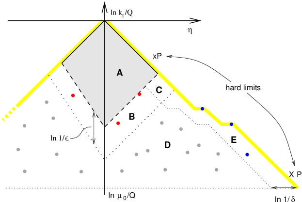
Figure 5: Analogue of fig. 2 for the case of an incoming leg (corresponding to positive rapidities). All emissions have already been clustered (as described in section 2.2.2). Emissions in region D contribute neither to the observable nor to the evolution of the PDF and can be neglected; emissions in E contribute to the PDF evolution but not to the observable; emissions in C contribute to both, but only at the NNLL level $\alpha_{{\textsc{s}}}^{n}L^{n-1}\ln\epsilon\ln\delta$; region B leads to the ${\cal{F}}(R^{\prime})$ function as in the case with only outgoing legs; and emissions are essentially forbidden in region A (except, potentially, close to the boundary with B), giving the usual double logarithmic $e^{-R(v)}$ suppression.

We subdivide the figure into a number of regions. As in fig. 2, we identify the region $V(k,\{\tilde{p}\})>v$, vetoed in the case of a single emission, now calling it region A. We also define a second boundary $V(k,\{\tilde{p}\})=\epsilon v$, again choosing $\epsilon\ll 1$, $\alpha_{{\textsc{s}}}\ln 1/\epsilon\ll 1$, below which it is safe to neglect emissions when evaluating the $\Theta$-function for the observable in eq. (179) (due to rIRC safety).

Additionally, we introduce a boundary parallel to the collinear limit, $1-y=\delta$, and choose $\delta\ll 1$, $\alpha_{{\textsc{s}}}\ln^{2}1/\delta\ll 1$ and also $\alpha_{{\textsc{s}}}\ln\epsilon\ln\delta\ll 1$. Emissions to the left of this boundary will not significantly modify the argument of the $\delta$-function on longitudinal momentum in eq. (179), because they have $y_{i}$ sufficiently close to $1$ that it can be ignored in the product of the $y_{i}$.

These two boundaries delineate a region D in fig. 5 in which emissions neither contribute to the observable, nor change the incoming parton momentum fraction. Therefore one can sum over them to directly cancel the corresponding part of the virtual corrections.

In the region $E$, the emissions do not contribute to the observable, however they do contribute to the argument of the $\delta$-function in eq. (179). So we make use of the fact that

$$q_{\delta}(x,\mu^{2})=\int dXq_{\delta}(X,\mu_{0}^{2})\sum_{n=0}^{\infty}\left(\prod_{i=1}^{n}\int[dk_{i}]\,|M^{2}_{I,rc}(k_{i})|\Theta(k_{ti}-k_{t,i+1})\Theta(1-y_{i}-\delta)\right)\times\\ \times\Theta(\mu-k_{t1})e^{-\int[dk]|M^{2}_{I,rc}(k)|\Theta(1-y-\delta)\Theta(\mu-k_{t})\Theta(k_{t}-\mu_{0})}\delta\Big{(}x-X\prod_{i}y_{i}\Big{)}\,,$$ (183)

(as can be verified by noting that for $\mu=\mu_{0}$ one obtains $q_{\delta}(x,\mu_{0}^{2})$ and that taking a derivative with respect to $\mu^{2}$, eq. (183) yields the single-logarithmic non-singlet DGLAP equation) and sum over all emissions in region E so as to rewrite eq. (179) as

$${\hat{f}}_{{\cal B},\delta}(v)=\int dX\>q_{\delta}(X,(\epsilon v)^{2/(a+b_{1})}Q^{2})\>\sum_{n=0}^{\infty}\left(\prod_{i=1}^{n}\int_{\epsilon v}[dk_{i}]\,|M^{2}_{I,rc}(k_{i})|\Theta(k_{ti}-k_{t,i+1})\right)\times\\ \times\Delta_{\epsilon v}(Q,k_{1},\ldots,k_{n},\mu_{0})\Theta(v-V(\{\tilde{p}\},k_{1},\ldots,k_{n}))\>\delta\Big{(}x-X\prod_{i}y_{i}\Big{)},$$ (184)

where the suffix $\epsilon v$, on both real and virtual corrections, indicates, as elsewhere that we consider only contributions satisfying $V(k,\{\tilde{p}\})>\epsilon v$. Note that in arriving at eq. (184) we have additionally made use of the fact that to within accuracy $\alpha_{{\textsc{s}}}^{n}L^{n-1}$ the slight mismatch between region E and the region defined by $y>1-\delta$, $(\epsilon v)^{1/(a+b_{1})}Q>k_{t}>\mu_{0}$ does not affect the single-logarithmic reconstruction of $q_{\delta}(X,(\epsilon v)^{2/(a+b_{1})}Q^{2})$ (it being a region of phase space of order $\alpha_{{\textsc{s}}}\ln^{2}\delta$). Note also that here our integration variable $X$ is no longer the momentum fraction of the parton extracted directly from the proton at scale $\mu_{0}^{2}$, but rather the momentum fraction after it has radiated all the emissions in E.

Next, we consider region C, where emissions can both modify the incoming momentum fraction and modify the value of the observable, the latter by an absolute amount of order $v$, or equivalently by a relative factor of order $1$ (but no more, since the observable is continuously global and rIRC safe). The effect of modifying the momentum fraction essentially amounts to further DGLAP evolution up to a scale of order $v^{1/(a+b_{1})}Q$ (equivalent to a NNLL contribution of order $\alpha_{{\textsc{s}}}\ln\epsilon(\alpha_{{\textsc{s}}}\ln v)^{n}$, which we include, and which through eq. (183) also causes the longitudinal momentum fraction for the PDF to become $x$), together potentially with an effective ${\cal{O}}\left(\alpha_{{\textsc{s}}}^{n}\ln^{n-1}v\right)$ coefficient function, again NNLL (which we shall neglect). Because of coherence, the dynamics of multiple soft-collinear emission is independent of both of these effects and so they will factorise from our result, which to NLL accuracy therefore becomes,

$${\hat{f}}_{{\cal B},\delta}(v)=q_{\delta}(x,v^{2/(a+b_{1})}Q^{2})\>\sum_{n=0}^{\infty}\left(\prod_{i=1}^{n}\int_{\epsilon v}[dk_{i}]\,|M^{2}_{I,rc}(k_{i})|\right)\\ \Delta_{\epsilon v}(Q,k_{1},\ldots,k_{n},\mu_{0})\Theta(v-V(\{\tilde{p}\},k_{1},\ldots,k_{n}))\,.$$ (185)

In this formula, for the specific observable depicted in fig. 5, one might worry that there are emissions in region B, with transverse momenta of the same order of magnitude as emissions in region E that have been removed. This could conceivably cause problems because of the identification of $z^{(1)}_{i}$ which depends on all emissions at higher scales. However, the relevant part of B corresponds to soft emissions, and our integration limits are directly on $z^{(1)}_{i}$, not on $y_{i}$ (since they come from the boundary of the incoming hemisphere and from the condition $V(k\{\tilde{p}\})=\epsilon v$). Using eq. (181), and the fact that $1-y_{i}\ll 1$, we have $dy_{i}/(1-y_{i})=dz^{(1)}_{i}/z^{(1)}_{i}$ and so $[dk_{i}]\,|M^{2}_{I,rc}(k_{i})|=[dk_{i}]\,|M^{2}_{rc}(k_{i})|$ (with $|M^{2}_{rc}(k_{i})|$ as defined in eq. (13)), we can integrate over these emissions independently of the pattern of emissions in region E.

A similar argument can be applied to the part of region A that is below transverse momentum scale $Qv^{\frac{1}{a+b_{1}}}$. However, above that scale the virtual corrections need to be integrated up to the hard collinear limit and some care is needed in evaluating $\Delta$, eq. (182). Since we discuss transverse momentum scales above $Qv^{\frac{1}{a+b_{1}}}$, we have that $m(k_{t})=0$. Observing that

$$\int_{0}^{1}dy\,p_{qq}(y)\,\Theta\Big{(}1-y-\frac{k_{t}}{2xE_{P}}\Big{)}=\int^{1}_{0}dz^{(1)}\,p_{gq}(z^{(1)})\,\Theta\Big{(}z^{(1)}-\frac{k_{t}}{2xE_{P}}\Big{)}\,,$$ (186)

one finds that the replacement $[dk_{i}]\,|M^{2}_{I,rc}(k_{i})|\to[dk_{i}]\,|M^{2}_{rc}(k_{i})|$ can be used right up to the hard collinear limit. Thus we may systematically rewrite eq. (185) in terms of $|M^{2}_{rc}(k)|$, removing also the ordering in $k_{t}$, to obtain

$${\hat{f}}_{{\cal B},\delta}(v)=q_{\delta}(x,v^{2/(a+b_{1})}Q^{2})\>\exp\left(-\int_{\epsilon v}[dk]\,|M^{2}_{rc}(k)|\,\right)\times\\ \times\sum_{n=0}^{\infty}\frac{1}{n!}\left(\prod_{i=1}^{n}\int_{\epsilon v}[dk_{i}]\,|M^{2}_{rc}(k_{i})|\right)\Theta(v-V(\{\tilde{p}\},k_{1},\ldots,k_{n}))\,.$$ (187)

While the precise sequence of our arguments relied on the fact that $b_{1}\geq 0$ (specifically, this led to region B and part of A being at similar transverse momenta to region E), eq. (187) applies independently of the value of $b_{1}$, as can be verified by repeating the analysis in the case of $b_{1}<0$.

Apart from the overall PDF factor (and the removal of emissions below $\epsilon v$), eq. (187) is identical to eq. (34), and so all the manipulations of section 2.2.3 may be repeated, to give

$${\hat{f}}_{{\cal B},\delta}(v)=q_{\delta}(x,v^{2/(a+b_{1})}Q^{2})\,e^{-R(v)}\,{\cal{F}}\,,$$ (188)

with $R(v)$ and ${\cal{F}}$ as evaluated in that section. Therefore the probability $f(v)$ includes the correction factor quoted in eq. (57).

E.2 Flavour singlet case

We finally discuss the extension of the above result to the flavour singlet-case. We shall use the index $\delta$ to denote the incoming parton flavour (as opposed to the hard process as a whole, as used elsewhere in the paper).

It would be tempting to simply extend eq. (179) so as to have the appropriate flavour matrix structure. However eq. (179) assumes an ordering in transverse momenta, while, as discussed in section 2.2 (see also chapter 5 of [52]), coherence actually implies that the colour factor for soft radiation is determined by the combination of emissions at smaller angles, not smaller transverse momenta. It is therefore useful to rewrite eq. (179) in terms of angular ordered emissions as follows (restricting our attention just to the incoming hemisphere),

$${\hat{f}}_{{\cal B},\delta}(v)=\int dX\>q_{\delta}(X,\mu_{0}^{2})\>\sum_{n=0}^{\infty}\left(\prod_{i=1}^{n}\int[dk_{i}]\,|M^{2}_{rc}(k_{i})|\Theta(\eta_{i+1}-\eta_{i})\overline{\Delta}(\eta_{i},\eta_{i+1})\right)\times\\ \times\overline{\Delta}(0,\eta_{1})\Theta(v-V(\{\tilde{p}\},k_{1},\ldots,k_{n}))\>\delta\Big{(}x-X\prod_{i}y_{i}\Big{)},$$ (189)

where in terms of angles virtual corrections become

$$\ln{\overline{\Delta}}(\eta_{i},\eta_{i+1})=-\int[dk]M^{2}_{I,rc}(k)\Theta(\eta-\eta_{i})\,\Theta(\eta_{i+1}-\eta)\,,$$ (190)

where in the evaluation of ${\overline{\Delta}}(\eta_{i},\eta_{i+1})$, the rapidity of emission $k$ can be expressed in terms of $y$ as $\eta=-\ln\frac{k_{t}}{2(1-y)xE_{P}}-\sum_{j=1}^{i}\ln y_{j}$. We have now a relation between $\mu_{0}^{2}$ and the smallest angular scale, $\eta_{n+1}=\ln 2xE_{P}/\mu_{0}-\sum_{j=1}^{n}\ln y_{j}$ and we continue to use eq. (181) to reconstruct the $z^{(1)}_{i}$ (and so the $\eta_{i}$) from the $y_{i}$.

The extension of eq. (189) to the flavour singlet case requires that one replace the unit flavour matrix element in eq. (189) with the appropriate, full flavour-singlet matrix structure

$${\hat{f}}_{{\cal B},\delta}(v)=\int dX\>\sum_{n=0}^{\infty}\left(\prod_{i=1}^{n}\int[dk_{i}]\,|M^{2}_{rc,\delta_{i}\delta_{i+1}}(k_{i})|\Theta(\eta_{i+1}-\eta_{i}){\overline{\Delta}}(\eta_{i},\eta_{i+1})\right)\times\\ \times\Theta(v-V(\{\tilde{p}\},k_{1},\ldots,k_{n}))\,{\overline{\Delta}}(0,\eta_{1})\,\delta_{\delta\delta_{1}}\>q_{\delta_{n+1}}(X,\mu_{0}^{2})\>\delta\Big{(}x-X\prod_{i}y_{i}\Big{)},$$ (191)

where we now have an index $\delta_{i}$ to denote the flavour of the exchanged parton at angular scales above that of emission $i$, and $\delta_{n+1}$ is the flavour of the incoming parton, and we sum over all flavours. The matrix element now has the structure

$$[dk_{i}]\,|M^{2}_{rc}(k_{i})|=\frac{\alpha_{{\textsc{s}}}(k_{t}^{2})}{2\pi}\frac{d\phi_{i}}{2\pi}\frac{dk_{ti}^{2}}{k_{ti}^{2}}dy_{i}\left(\begin{array}[]{cc}C_{F}\,p_{qq}(y_{i})&2n_{\!f}T_{R}\,p_{qg}(y_{i})\\ C_{F}\,p_{gq}(y_{i})&C_{A}[p_{gg}(y_{i})+p_{gg}(1-y_{i})]\end{array}\right),$$ (192)

where the elementary splitting functions, $p_{\delta\delta^{\prime}}$, are as defined elsewhere (after eqs. (11) and (180), and eqs. (59)) and the left and right-hand columns act respectively on the quark singlet ($d+\bar{d}+u+\bar{u}+\ldots$) and gluon distributions.

In term of angles, virtual corrections, which are diagonal in flavour space, give

$$\ln{\overline{\Delta}}(\eta_{i},\eta_{i+1})=-\int\frac{dk_{t}^{2}}{k_{t}^{2}}\frac{\alpha_{{\textsc{s}}}(k_{t}^{2})}{2\pi}\,dy\,\Theta(\eta-\eta_{i})\,\Theta(\eta_{i+1}-\eta)\times\\ \times\left(\begin{array}[]{cc}C_{F}\,p_{qq}(y)&0\\ 0&C_{A}\,p_{gg}(1-y)+n_{\!f}T_{R}\,p_{qg}(y)\end{array}\right),$$ (193)

where, as above, $\eta=-\ln\frac{k_{t}}{2(1-y)xE_{P}}-\sum_{j=1}^{i}\ln y_{j}$.

There are some subtleties to be aware of in the relation between eq. (192) and for example (59) — in the outgoing case of eq. (59) there is a symmetry between the two partons coming out of a $g\to gg$ or $g\to q\bar{q}$ splitting (if one neglects the difference between quark and antiquark, as is the case for an event shape). In the incoming case, the symmetry is broken by the fact that one of the descendants from the splitting will enter the hard process while the other will go into the final state, and we need to include separate contributions for the cases where it is the first or the second of the splitting products that continues into the hard process. It is for this reason that in the real matrix element eq. (192) (but not the virtual part) we need to write $p_{gg}(y_{i})+p_{gg}(1-y_{i})$, and include a factor of $2n_{\!f}$ in front of $p_{qg}$, rather than just $n_{\!f}$ (making use of the explicit $y\leftrightarrow 1-y$ symmetry of $p_{qg}$), and similarly that we need to include both the $p_{qq}$ and the $p_{gq}$ splittings (whereas previously we had just one of them).

One can now repeat the flavour non-singlet analysis given above. There are certain other small differences, for example in region E the final DGLAP evolution that we obtain corresponds to angular-ordered DGLAP evolution rather than transverse-momentum ordered (this is known to give only subleading, $\alpha_{{\textsc{s}}}^{n}L^{n-1}$ differences, potentially enhanced by $\ln^{2}X/x$, such terms being in any case neglected in eq. (192)). However the main thrust of the analysis persists, one can still separate the different regions, and one obtains a factorised $q_{\delta}(x,v^{2/(a+b_{1})}Q^{2})$ contribution from E, ${\cal{F}}$ from real (virtual) emissions in A and B (just B), $e^{-R(v)}$ from the integral over virtual terms in A, NNLL contributions from C and terms suppressed by powers of $\epsilon$ or $\delta$ from D. Furthermore the colour factor associated with $e^{-R(v)}$ and ${\cal{F}}$ is that of the parton flavour $\delta$ entering the hard process, since all logarithmically enhanced flavour-changing branchings are in E which is at smaller angles than regions A and B.

Our result for ${\hat{f}}_{{\cal B},\delta}(v)$ is therefore given by eq. (188) even in the singlet case. The final step is to relate this to $f_{{\cal B},\delta}(v)$ discussed elsewhere in the text. Comparing eqs. (3), (177) and (178) one sees that

$$f_{{\cal B},\delta}(v)=\frac{{\hat{f}}_{{\cal B},\delta}(v)}{q_{\delta}(x,Q^{2})}=\frac{q_{\delta}(x,v^{2/(a+b_{1})}Q^{2})}{q_{\delta}(x,Q^{2})}e^{-{\cal{R}}(v)}{\cal{F}}\,,$$ (194)

which is the result quoted in eq. (57).

Appendix F Further examples of rIRC unsafety

Here, with the help of some resolution thresholds in jet-clustering algorithms, we illustrate three cases of IRC safe observables that are rIRC unsafe. One example is devoted to each of the rIRC conditions of section 3.1.

F.1 Jade jet algorithm: $\boldsymbol{E}$-scheme

Jet clustering algorithms are widely studied observables. They typically involve a distance measure $y_{ij}$ between two (pseudo)particles and a clustering sequence in which one searches for the particle pair with the smallest $y_{ij}$, clusters it into a single pseudoparticle and then repeats the clustering procedure until all remaining pairs have $y_{ij}>y_{cut}$, where $y_{cut}$ is the jet resolution parameter. From the point of view of this article, the observable that is typically of interest is the distribution of the value of $y_{cut}$ that demarcates the threshold between an $n$ and an $n+1$-jet event.

Of particular interest is the family of JADE algorithms [33] because it represents the only example of an observable for which the double logarithms have been found, analytically, not to exponentiate [34, 35]. Taking the definition used in [34], the distance measure is

$$y_{ij}=\frac{(q_{i}+q_{j})^{2}}{Q^{2}}\,,$$ (195)

and the recombination scheme is the $E$-scheme, $q_{ij}=q_{i}+q_{j}$. It is straightforward to show that, in the two-jet limit, at the level of a single soft and collinear emission, the $2$-to-$3$ jet threshold resolution, $y_{3}$ is identical to $\tau=1-T$,

$$a=1=b_{\ell}=d_{\ell}=g_{\ell}(\phi)=1\,,\qquad\quad\ell=1,2\,.$$ (196)

As above, we use ${\bar{v}}$ and $\xi_{i}$ to parametrise an emission $\kappa_{i}({\bar{v}})$, giving

$$\ln\frac{\kappa_{ti}({\bar{v}})}{Q}=\left(1-\frac{\xi_{i}}{2}\right)\ln{\bar{v}}\,,\qquad\eta_{i}({\bar{v}})=-\frac{\xi_{i}}{2}\ln{\bar{v}}\,.$$ (197)

Let us now consider two emissions $\kappa_{1}({\bar{v}})$ and $\kappa_{2}({\bar{v}})$ collinear to the two different legs ($1$ and $2$ respectively). One has (ignoring $y_{p_{1}p_{2}}\simeq 1$)

$$y_{\kappa_{1}p_{1}}=y_{\kappa_{2}p_{2}}={\bar{v}}\,,\quad y_{\kappa_{1}p_{2}}={\bar{v}}^{1-\xi_{1}}\,,\quad y_{\kappa_{2}p_{1}}={\bar{v}}^{1-\xi_{2}}\,,\quad y_{\kappa_{1}\kappa_{2}}={\bar{v}}^{2-\xi_{1}-\xi_{2}}\,,\quad$$ (198)

and recombination will occur between $\kappa_{1}$ and $\kappa_{2}$ if $\xi_{1}+\xi_{2}<1$. If this is the case, then two recombinations are now possible, with distance measures

$$y_{\kappa_{12}p_{1}}=y_{\kappa_{1}p_{1}}+y_{\kappa_{2}p_{1}}+y_{\kappa_{1}\kappa_{2}}\simeq y_{\kappa_{2}p_{1}}\,,\quad y_{\kappa_{12}p_{2}}=y_{\kappa_{1}p_{2}}+y_{\kappa_{2}p_{2}}+y_{\kappa_{1}\kappa_{2}}\simeq y_{\kappa_{1}p_{2}}\,,$$ (199)

and as a result the three-jet resolution parameter will be

$$y_{3}\left(\{\tilde{p}\},\kappa_{1}({\bar{v}}),\kappa_{2}({\bar{v}})\right)\simeq{\bar{v}}^{1-\min(\xi_{1},\xi_{2})}\,,\qquad\quad\xi_{1}+\xi_{2}<1\,,\;\ell_{1}\neq\ell_{2}\,.$$ (200)

This does not scale as ${\bar{v}}$, so the limit eq. (71) is not finite, therefore the observable fails the first rIRC test. One can verify that this breakdown of scaling as ${\bar{v}}$ occurs in a double logarithmic region, in accord with the known result [34] that the E-scheme JADE jet-resolution distribution fails to exponentiate at the double-logarithmic level. An interesting demonstration of this point is in the evaluation of ${\cal{F}}$, or more specifically of its expansion in powers of $R^{\prime}$, which starts at $R^{\prime 2}$, as discussed in appendix A.2. The $\bar{v}\to 0$ limits of ${\cal{F}}$ and ${\cal{F}}_{2}$ diverge. This divergence can be thought of as somewhat analogous to the divergence of NLO corrections for an IRC unsafe observable.

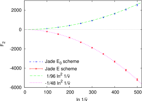
Figure 6: Calculation of ${\cal{F}}_{2}$ for the Jade $y_{3}$ resolution parameter in the $E$ and $E_{0}$ recombination schemes. The points have been calculated by Monte Carlo evaluation of eq. (119).

Additionally the nature of the divergence provides information about the violation of exponentiation. Figure 6 shows ${\cal{F}}_{2}$ evaluated as a function of $\bar{v}$, using eq. (119) (in whose derivation care has been taken to retain all leading logarithmic dependence on $\bar{v}$). One sees that ${\cal{F}}_{2}$ diverges as $\ln^{2}1/{\bar{v}}$, which is indicative of the fact that the lack of rIRC safety is associated with ‘multiple-emission’ effects being relevant not at order $\alpha_{{\textsc{s}}}^{2}L^{2}$, but rather at order $\alpha_{{\textsc{s}}}^{2}L^{4}$.

Using the following leading order, double logarithmic approximations

$$R(\bar{v})=\frac{\alpha_{{\textsc{s}}}C_{F}}{\pi}\ln^{2}\frac{1}{\bar{v}}\,,\qquad\quad R^{\prime}(\bar{v})=2\frac{\alpha_{{\textsc{s}}}C_{F}}{\pi}\ln\frac{1}{\bar{v}}\,,$$ (201)

and comparing to the double logarithmic result in [34], one obtains that the deviation from exponentiation is expected to be of the form

$$f(v)=1-R(v)+\frac{5}{6}\frac{R^{2}(v)}{2}+\ldots\,.$$ (202)

If one tries to account for this for by a function ${\cal{F}}(R^{\prime},v)=1+{\cal{F}}_{2}(v)R^{\prime}(v)^{2}+\ldots$ multiplying $e^{-R(v)}$, then ${\cal{F}}_{2}(v)R^{\prime}(v)^{2}$ should be equal to $-R(v)^{2}/12$, i.e.

$${\cal{F}}_{2}(v)=-\frac{1}{48}\ln^{2}\frac{1}{v}\,.$$ (203)

This result is also plotted in fig. 6 and coincides well with the numerical evaluation based on eq. (119).

F.2 Jade jet algorithms: $\boldsymbol{E}_{0}$-scheme

As it happens, the $E$-scheme as defined above is rarely used experimentally. More common is the $E_{0}$ scheme (see for example [75]) where particles are recombined according to

$$E_{ij}=E_{i}+E_{j}\,,\qquad{\vec{q}}_{ij}=\frac{E_{ij}}{|\vec{q}_{i}+\vec{q}_{j}|}\left(\vec{q}_{i}+\vec{q}_{j}\right)\,.$$ (204)

This has been studied analytically in [35, 36]. One can repeat the analysis of section F.1, and one finds that the problem with the first rIRC condition disappears because $\min_{\ell=1,2}y_{\kappa_{12}p_{\ell}}\simeq\max\left(y_{\kappa_{1}p_{1}},y_{\kappa_{2}p_{2}}\right)\simeq{\bar{v}}$ and so the limit eq. (71) is well-defined and finite.

One still needs however to verify the other conditions, eqs. (72). A configuration that is of interest here is that with two soft and collinear gluons, $\kappa_{1}({\bar{v}})$ and $\kappa_{2}(\zeta_{2}{\bar{v}})$ in the same hemisphere (say that containing leg $1$). Note that we have reintroduced $\zeta_{2}$ ($\leq 1$). Let us assume $\kappa_{2}(\zeta_{2}{\bar{v}})$ is much more collinear to the hard parton than $\kappa_{1}({\bar{v}})$, $(\zeta_{2}{\bar{v}})^{\xi_{2}/2}\ll{\bar{v}}^{\xi_{1}/2}$. For the first recombination, the various possible clusterings include,

$$y_{{\kappa_{1}}p_{1}}={\bar{v}}\,,\quad y_{{\kappa_{2}}p_{1}}=\zeta_{2}{\bar{v}}\,,\quad y_{{\kappa_{1}}{\kappa_{2}}}={\bar{v}}(\zeta_{2}{\bar{v}})^{1-\xi_{2}}\,,$$ (205)

and when $\zeta_{2}>{\bar{v}}^{\frac{1-\xi_{2}}{\xi_{2}}}$, the first recombination occurs between $\kappa_{1}$ and $\kappa_{2}$. Let us suppose that this is the case. Then, as long as $\kappa_{t1}\ll\kappa_{t2}$, i.e. ${\bar{v}}^{1-\xi_{1}/2}\ll(\zeta_{2}{\bar{v}})^{1-\xi_{2}/2}$, the energy and transverse momentum of the $\kappa_{12}$ pseudo-particle will be dominated by $\kappa_{2}$ and we will have

$$y_{\kappa_{12}p_{1}}\simeq y_{\kappa_{2}p_{1}}=\zeta_{2}{\bar{v}}\,.$$ (206)

Let us now examine this result in the context of eq. (72a). To obtain the left-hand side we should first take ${\bar{v}}\to 0$. Our requirement on $\kappa_{2}(\zeta_{2}{\bar{v}})$ being more collinear than $\kappa_{1}$ simply implies $\xi_{2}>\xi_{1}$, as does the condition $\kappa_{t1}\ll\kappa_{t2}$; then the first recombination is automatically $\kappa_{1}\kappa_{2}$ and we obtain the result that

$$\lim_{\zeta_{2}\to 0}\lim_{{\bar{v}}\to 0}\frac{1}{{\bar{v}}}y_{3}(\{\tilde{p}\},\kappa_{1}({\bar{v}}),\kappa_{2}(\zeta_{2}{\bar{v}}))=\Theta(\xi_{1}-\xi_{2})\,.$$ (207)

In contrast the right-hand side of (72a) is

$$\lim_{{\bar{v}}\to 0}\frac{1}{{\bar{v}}}y_{3}(\{\tilde{p}\},\kappa_{1}({\bar{v}}))=1\,.$$ (208)

Thus eq. (72a) does not hold and the $E_{0}$ Jade algorithm fails on the second of the recursive IRC safety conditions. Despite the failure being on a different condition compared to the observables discussed above, here too the nature of the violation is such that exponentiation is broken at the level of $\alpha_{{\textsc{s}}}^{2}L^{4}$ corrections. As in the discussion for the $E$ scheme, one can evaluate the second order contribution to ${\cal{F}}$ as a function of $\ln\bar{v}$, and compare it with the known analytical result of [35],

$$f(v)=1-R(v)+\frac{13}{12}\frac{R^{2}(v)}{2}+\ldots\,,$$ (209)

corresponding to ${\cal{F}}_{2}(v)=\frac{1}{96}\ln^{2}\frac{1}{v}$. The comparison is shown in figure 6 and, as for the $E$ scheme, one finds good agreement.

A final subtle, but non-trivial point to note here concerns the requirement that $\kappa_{t2}\gg\kappa_{t1}$ for eq. (206) to hold — though we have called our condition recursive infrared collinear safety, in some cases the limits that we take, notably here $\zeta_{2}\to 0$, still leave the ‘infrared and collinear’ particle, $\kappa_{2}$, harder (larger transverse momentum, larger energy, albeit smaller angle) than the supposedly dominant contribution $\kappa_{1}$. This apparent paradox is closely related to the fact that we use a single quantity, the value of $V(\{\tilde{p}\},\kappa)$, to define the degree to which an emission $\kappa$ is infrared and collinear. This controls only some combination of the infrared and collinear limits, but not the two independently (the remaining degree of freedom is set by $\xi$). Thus two emissions which may be ordered according to one given soft-collinear criterion, $V(\{\tilde{p}\},\kappa_{2})<V(\{\tilde{p}\},\kappa_{1})$ are not necessarily ordered according to some other criterion.

F.3 Geneva jet algorithm

Let us close this discussion of rIRC safety for jet algorithms by examining the Geneva jet clustering algorithm [76]. It is similar in spirit to the preceding algorithms, except that the distance measure is given by

$$y_{ij}=\frac{8}{9}\frac{E_{i}E_{j}(1-\cos\theta_{ij})}{(E_{i}+E_{j})^{2}}\,,$$ (210)

the essential change being the replacement of $Q^{2}$ in the denominator with $(E_{i}+E_{j})^{2}$. For events with two hard partons and one soft collinear emission, this only changes the normalisation of the $y_{ij}$ compared to the Jade family of algorithms, and one has

$$a_{\ell}=b_{\ell}=g_{\ell}(\phi)=1\,,\qquad d_{\ell}=\frac{16}{9}\,,\qquad\ell=1,2\,.$$ (211)

The Geneva algorithm is interesting when a soft collinear emission, $\kappa_{1}({\bar{v}})$, is split collinearly, $\kappa_{1}({\bar{v}})\to\{\kappa_{1_{a}},\kappa_{1_{b}}\}({\bar{v}},\mu)$, with a small normalised pair invariant mass, $\mu^{2}=(\kappa_{1_{a}}+\kappa_{1_{b}})^{2}/\kappa_{t1}^{2}\ll 1$, and fractions $z_{a}$ and $z_{b}=1-z_{a}$ of the parent momentum. The various possible recombinations include (assuming $\kappa_{1}$ is collinear to leg $1$)

$$y_{\kappa_{1_{a}}p_{1}}=z_{a}y_{\kappa_{1}p_{1}}=z_{a}{\bar{v}}\,,\qquad y_{\kappa_{1_{b}}p_{1}}=z_{b}y_{\kappa_{1}p_{1}}=z_{b}{\bar{v}}\,,\qquad y_{\kappa_{1_{a}}\kappa_{1_{b}}}=\frac{16}{9}e^{-2\,\eta_{1}}\mu^{2}\,.$$ (212)

Whereas one would expect a ‘good’ jet algorithm to first recombine $\kappa_{1_{a}}$ and $\kappa_{1_{b}}$, what actually happens (as was first observed in [35]), for ${\bar{v}}\ll\mu^{2}$, is that for $z_{a}>z_{b}$ first $\kappa_{1_{b}}$ is recombined with $p_{1}$, and then $\kappa_{1_{a}}$ is recombined with $p_{1}$ (inversely for $z_{a}<z_{b}$), giving

$$V(\{\tilde{p}\},\{\kappa_{1_{a}},\kappa_{1_{b}}\}({{\bar{v}}},\mu))=\left\{\begin{array}[]{rc}{\bar{v}}\,,&\qquad\frac{16}{9}e^{-2\,\eta_{1}}\mu^{2}\lesssim\min(z_{a},z_{b}){\bar{v}}\,,\\ \max(z_{a},z_{b}){\bar{v}}\,,&\qquad\frac{16}{9}e^{-2\,\eta_{1}}\mu^{2}\gtrsim\min(z_{a},z_{b}){\bar{v}}\,.\end{array}\right.$$ (213)

As a result the two limits in eq. (72b) differ,

$$\lim_{\mu\to 0}\lim_{{\bar{v}}\to 0}\frac{1}{\bar{v}}V(\{\tilde{p}\},\{\kappa_{1_{a}},\kappa_{1_{b}}\}({{\bar{v}}},\mu))=\max(z_{a},z_{b})\,,\qquad\lim_{{\bar{v}}\to 0}\frac{1}{\bar{v}}V(\{\tilde{p}\},\kappa_{1}({\bar{v}}))=1\,,$$ (214)

and the observable fails on the second part of the second rIRC safety criterion. The failure only occurs for hard collinear (non soft) secondary splittings. Furthermore the two limits in eq. (214) differ by at most a factor of order $1$ (specifically by at most $1/2$). As a result it is possible to show that the full resummed distribution for the Geneva $y_{3}$ resolution parameter differs from the master formula (for which all elements are well defined) by terms $\alpha_{{\textsc{s}}}^{n}L^{n}$. We note that in contrast to the situation with the Jade algorithm, the rIRC unsafety of the Geneva algorithm does not manifest itself through a divergent infrared dependence in the integrals for ${\cal{F}}$, because the integrations for secondary collinear splitting have already been carried out analytically, assuming rIRC safety. Accordingly the ${\cal{F}}$ function is well defined (${\cal{F}}(R^{\prime})=1$).

Appendix G Infrared and collinear safety

In the automated approach discussed in this paper, we do not actually explicitly test for the full infrared and collinear (IRC) safety of the observable — we rather assume that the user of the program is able to correctly design and code IRC safe observables.

We believe though that it is instructive to discuss some aspects of IRC safety, for two main reasons. Firstly, IRC safety turns out to be somewhat more subtle than is usually reflected in ‘textbook’ discussions. Secondly many of the issues that arise concerning IRC safety are relevant also for rIRC safety, since the two conditions have numerous similarities.

G.1 Standard discussions of IRC safety

The general definition of IRC safety is that it is the necessary and sufficient condition that an observable has to satisfy in order for its distribution to be calculable and finite, order-by-order within perturbation theory.

For practical purposes however it is more convenient to attempt to cast IRC safety in terms of certain properties of the observable’s functional dependence on the emission momenta, because IRC safety can then be tested without explicitly calculating order by order perturbative predictions for the observable. An example of a definition (taken from p. 72 of [52]) is

For the [variable’s distribution] to be calculable in perturbation theory, the variable should be infra-red safe, i.e. insensitive to the emission of soft or collinear gluons. In particular if ${\vec{p}}_{i}$ is any momentum occurring in its definition, it must be invariant under the branching

$${\vec{p}}_{i}\to{\vec{p}}_{j}+{\vec{p}}_{k}$$ (215)

whenever ${\vec{p}}_{j}$ and ${\vec{p}}_{k}$ are parallel or one of them is small.

One notes that there are two parts to this definition, the first being somewhat hand-waiving, the second appearing more precise. In certain other texts, only the second part is given, for example (from section IV.A.2 of [77])

[…] That is to say, the measurement should not distinguish between a final state in which two particles are collinear and the final state in which these two particles are replaced by one particle carrying the sum of the momenta of these collinear particles. Similarly, the measurement should not distinguish between a final state in which one particle has zero momentum and the final state in which this particle is omitted entirely.

The argument that a cross section specified by functions $\cal S$ with this property does not have infrared divergences may be understood as an extension of the KLN theorem […]

G.2 Difficulties with standard definitions

It is instructive to examine these (and other) definitions of IRC safety for some ‘designer’ observables in $e^{+}e^{-}$ processes. These will be constructed in terms of the $n$-jet threshold resolution parameters, $y_{n}$, in the Durham jet algorithm [18]. Specifically, $y_{n}$ is the value of $y_{\mathrm{cut}}$ below which one has an $n$ jet event, and above which an $(n-1)$-jet event. Individually, all the $y_{n}$ are IRC safe observables.

Let us start by considering the following observable,

$$V=(1+\Theta(y_{5}-y_{4}^{2}))\,y_{3}\,,\qquad(\mbox{if $y_{4}=0$: $V=y_{3}$})\,.$$ (216)

It is non-zero starting from events with $3$ partons. If a fourth parton is added then the observable is identical to $y_{3}$ and so appears to be IRC safe. Adding a fifth parton and making it soft or collinear to one of the other emissions, then $\Theta(y_{5}-y_{4}^{2})$ will be zero and again we will have the appearance of IRC safety.

Now let us examine what happens if we integrate over the momenta of partons $4$ and $5$, taking them to be ordered. Assuming that they are emitted off different (hard) partons, we can approximate the phase space for each of them as $dy_{i}/y_{i}\ln 1/y_{i}$. We also schematically write the phase space and matrix element for the emission of the hard gluon $y_{3}$ $dy_{3}|M^{2}(y_{3})|$. The mean value of $V$ then gets an NNLO contribution which schematically has the form

$$\langle V\rangle_{\mathrm{NNLO}} \sim\alpha_{{\textsc{s}}}^{3}\int dy_{3}|M^{2}(y_{3})|\int^{y_{3}}\frac{dy_{4}}{y_{4}}\ln\frac{1}{y_{4}}\int^{y_{4}}\frac{dy_{5}}{y_{5}}\ln\frac{1}{y_{5}}\left[(1+\Theta(y_{5}-y_{4}^{2}))y_{3}-y_{3}\right]$$ (217a)

$$\sim\alpha_{{\textsc{s}}}^{3}\int dy_{3}M^{2}(y_{3})y_{3}\int^{y_{3}}\frac{dy_{4}}{y_{4}}\ln\frac{1}{y_{4}}\int^{y_{4}}_{y_{4}^{2}}\frac{dy_{5}}{y_{5}}\ln\frac{1}{y_{5}}\,,$$ (217b)

where in the first line the rightmost term in square brackets accounts for the combined one and two-loop virtual corrections. There is an infinite region of phase space for $y_{4}$ and $y_{5}$ where the real and virtual contributions do not fully cancel. So even though the observable is insensitive to any extra single arbitrarily soft or collinear emission (the condition often used to characterise IRC safety, as in [77]), it has a sensitivity to specific combinations of multiple extra arbitrarily infrared and collinear emissions, and this is sufficient to make it IRC unsafe.

It would be interesting to find a definition that would correctly identify eq. (216) as IRC unsafe, but that is more precise than, say, the generic requirement of ‘insensitivity to the emission of soft or collinear gluons’ of [52] and which therefore can serve as a basis for automated testing of IRC safety. As we shall see however, this is not a simple task.

G.3 Search for a rigorous formulation of IRC safety

As a first attempt, let us consider the following definition, inspired somewhat by the mathematical definition of a limit. First we introduce some distance measure, which parametrises the degree of collinearity of a pair of partons, or the softness of a parton (the distance measure could be the relative $k_{t}$ of the pair, or their invariant mass).

Version 1

Given almost any fixed set of partons (which we refer to as the ‘hard’ partons) and any value $n$, then for any $x$, however small, there should exist an $\epsilon$ such that branching the partons so as create up to $n$ extra soft or collinear emissions, each emission being at a distance of no more than $\epsilon$ from the nearest ‘hard’ parton, then the value of the observable does not change by more than $x$.

It is straightforward to see that the observable eq. (216) violates this condition.

The issue of sensitivity to multiple soft or collinear emissions is however not the only problem that arises when attempting to define a general IRC safety condition. Also relevant for example is the question of how quickly the effect of an emission disappears as it is made soft or collinear.

If one defines

$$V=y_{3}\left(1+\Theta(y_{4})\ln^{-q}\frac{1}{y_{4}}\right)\,,\qquad q>0\,,$$ (218)

then $V$ tends to $y_{3}$ in the limit $y_{4}\to 0$ (as in eq. (216), this and all subsequent observables are defined to be $V=y_{3}$ if $y_{4}=0$.). Specifically, if we take as our distance measure the squared relative transverse momentum (normalised to the hard scale $Q$), then in our IRC definition given above, however small an $x$ we choose, it suffices to take $\epsilon\equiv y_{4}<e^{-1/x^{1/q}}$ to ensure that any recombination will not change $V$ by more than $xy_{3}$.

As we have already discussed, the phase space associated with a fourth parton, expressed in terms of $y_{4}$ itself, goes roughly as $dy_{4}/y_{4}\ln 1/y_{4}$ for each of the three harder partons to which parton 4 can be collinear. If one attempts to calculate the contribution to the mean value from the integral over this phase space, including the subtraction of the virtual terms, one finds an order $\alpha_{{\textsc{s}}}^{2}$ contribution of the form

$$\langle V\rangle_{\mathrm{NLO}}\sim\alpha_{{\textsc{s}}}^{2}\int dy_{3}M^{2}(y_{3})\int^{y_{3}}\frac{dy_{4}}{y_{4}}\ln\frac{1}{y_{4}}\left[y_{3}\left(1+\ln^{-q}\frac{1}{y_{4}}\right)-y_{3}\right]\,.$$ (219)

This is divergent for $q<2$. At higher orders, since one effectively includes extra logarithms in the numerator (for example from the integrations that lead to the running of the coupling), one finds that however large a value we take for $q$, there will be some fixed order beyond which it is not possible to calculate the perturbative corrections to the mean value of $V$.

This suggests therefore that any corrections to an observable from extra emissions should vanish at least as fast as a power of the collinearity or softness of those emissions. This can be incorporated into Version 1 of our IRC definition, as follows:

Version 2

Given almost any fixed set of partons (which we refer to as the ‘hard’ partons) and any value $n$, then for any $x$, however small, there should exist an $\epsilon$ such that branching the partons so as create up to $n$ extra soft or collinear emissions, each emission being at a distance of no more than $\epsilon$ from the nearest ‘hard’ parton, then the value of the observable does not change by more than $x$.

Furthermore there should exist a positive power $p$ such that for small $x$, $\epsilon$ can always be taken greater than $x^{p}$.

One can straightforwardly verify that the observable of eq. (218) is correctly classified as unsafe with such a formulation of the IRC condition.

One of the patterns that the reader may see emerging from our discussion so far is that for each definition or IRC safety, one is able to design an observable that is incorrectly classified, requiring that one further refine the definition. Unfortunately this is a major difficulty, with even Version 2 of our definitions suffering from this problems.

The difficulty can be illustrated with the following set of observables,

$$V =y_{3}(1+\Theta(y_{4}-|\cos\theta_{24}|))\,,$$ (220)

$$V =y_{3}(1+\Theta(y_{4}-|\cos\theta_{23}|))\,,$$ (221)

$$V =y_{3}\left(1+\frac{\Theta(y_{4}-|\cos\theta_{23}|)}{y_{4}}\right)\,,$$ (222)

where $\theta_{ij}$ is the angle between jets $i$ and $j$ after clustering to $\max\{i,j\}$ jets and with jets numbered such such that $E_{i}>E_{i+1}$.

The first observable is IRC safe, because the extra $\Theta$-function term only contributes significantly in the logarithmic integration over $y_{4}$ when $\cos\theta_{24}$ is close to zero (a rare occurrence). It is however classified as IRC unsafe according to Version 2 of our condition, because if one adds an emission ($4$) such that it is exactly perpendicular to jet $2$ then however soft it is, it changes the value of the observable by a factor of $2$.

The second observable, eq. (221), is quite similar, and in particular is also IRC safe. Unlike eq. (220), it is correctly classified by Version 2 of our IRC condition. This is because $\epsilon$ is to be found for a given fixed configuration of hard momenta (in particular a given fixed value of $\theta_{23}$). It is not necessary that the same $\epsilon$ be valid for all hard momenta. Accordingly, however close $\theta_{23}$ is to zero, one can always find an appropriate value of $\epsilon$ for a given $x$. An exception occurs for $\theta_{23}=0$, however this corresponds to a region of zero measure in phase space, and is an allowed exception insofar as we required that the condition be true for almost any set of hard partons.

The third observable, eq. (221), also passes the test — the presence of $y_{4}$ in the denominator does not change one’s ability to find a point at which the effect of the fourth emission disappears. However it does change the integrability properties, since the presence of the $1/y_{4}$ factor compensates the reduced $\theta_{23}$ phase-space, leading to a divergent NLO contribution,

$$\langle V\rangle_{\mathrm{NLO}} \sim\alpha_{{\textsc{s}}}^{2}\int\!\!dy_{3}\,d\theta_{23}\,|M^{2}(y_{3},\theta_{23})|\int^{y_{3}}\!\frac{dy_{4}}{y_{4}}\ln\frac{1}{y_{4}}\left[y_{3}\left(1+\frac{\Theta(y_{4}-|\cos\theta_{23}|)}{y_{4}}\right)\!-\!y_{3}\right]$$ (223a)

$$\sim\alpha_{{\textsc{s}}}^{2}\int dy_{3}\,d\theta_{23}\,|M^{2}(y_{3},\theta_{23})|\,\frac{y_{3}\ln(1/\cos\theta_{23})}{\cos\theta_{23}}\,.$$ (223b)

For each of the mis-classifications identified above one could envisage some workaround that would solve the problem: for example allowing a subset of soft and collinear emissions to violate the IRC condition, as long as the subset’s measure is sufficiently limited; or requiring the observable’s value to be bounded.

But in the absence of a formal derivation of the resulting IRC condition, a doubt will always persist as to its general validity. Such a formal derivation might well be inspired by mathematical statements concerning the properties required of multivariate functions in order for them to be integrable. However that is beyond the scope of this article.

Let us finally comment on recursive IRC safety in the light of this discussion. Eqs. (72) for recursive IRC safety are similar to formulations of normal IRC safety in terms of a single emission that is made soft or collinear. The preamble to the discussion of rIRC safety attempts instead to give a general statement, somewhat analogous to that for IRC safety in [52]. The former is more understandable insofar as it appears more precise. One should however be aware of its limitations. For example in eq. (37), we have explicitly seen the need for the observable to be insensitive with respect to the removal of multiple relatively much softer emissions.

Appendix H Divergences of ${\cal{F}}$

H.1 General considerations

To obtain a more general understanding, than was given in section 3.4, of the contexts in which divergences can appear, it is useful to consider the case of the broadening with respect to the photon axis in the Breit-frame current hemisphere of DIS, $B_{zE}$. From the analytical studies in [24], one can write $B_{zE}$ in terms of the soft and collinear emissions, $k_{i}$, as

$$B_{zE}=\frac{1}{Q}\left(|{\vec{k}}_{t,\cal{H_{C}}}+{\vec{k}}_{t,\cal{H_{R}}}|+\sum_{i\in\cal{H_{C}}}|{\vec{k}}_{ti}|\right)\,,\qquad{\vec{k}}_{t,\cal{H_{R}}/\cal{H_{C}}}=\sum_{i\in\cal{H_{R}}/\cal{H_{C}}}{\vec{k}}_{ti}\,,$$ (224)

where $\cal{H_{R}}$ and $\cal{H_{C}}$ are the remnant and current hemispheres (associated respectively with legs $1$ and $2$) and the notation $\cal{H_{R}}/\cal{H_{C}}$ means either $\cal{H_{R}}$ or $\cal{H_{C}}$. For $B_{zE}$ to be small it is necessary to suppress emissions on leg $2$ (since there are no cancellations in $\sum_{i\in\cal{H_{C}}}|{\vec{k}}_{ti}|$), while through a cancellation in the 2-dimensional vector sum, emissions on leg $1$ can contribute little overall to $B_{zE}$ even if individually they have large transverse momenta. Accordingly, for configurations in which the hardest emission is on leg $1$, there is a small-$y$ contribution to ${\cal{P}}(y)$ of the form

$${\cal{P}}(y)\sim y^{2}\cdot y^{C_{2}r^{\prime}_{2}}\,,\qquad y\to 0\,,$$ (225)

where the first factor is that associated with the cancellation in the vector sum, while the second is associated with the Sudakov suppression for emissions from leg $2$.

More generally there are observables for which cancellations can occur for emissions off a subset $s$ of the legs, while the complementary subset of legs ($\bar{s}$) shows no cancellations. In such a case, assuming in analogy with before that there is a power $p$ associated with the structure of the cancellations on set $s$, then

$${\cal{P}}(y)\sim y^{p}\cdot y^{R^{\prime}_{\bar{s}}}\,,\qquad y\to 0\,,\qquad R^{\prime}_{s/\bar{s}}=\sum_{\ell\in{s/\bar{s}}}C_{\ell}r^{\prime}_{\ell}\,.$$ (226)

This gives a divergence at $R^{\prime}=p+R^{\prime}_{\bar{s}}$ or equivalently $R^{\prime}_{s}=p$. For the case of $B_{zE}$ this corresponds to $R^{\prime}_{s}=2$ or equivalently, $R^{\prime}=4$.

Such arguments can also be extended to cases where there are several subsets of legs subject separately to cancellations, $s_{1}$, $s_{2}$, …, each being associated with a power $p_{i}$. In such a situation, if the hardest emission is from a leg belonging to set $s_{i}$, then there is a contribution to ${\cal{P}}(y)$ for small $y$ of the form

$$y^{p_{i}}\cdot y^{R^{\prime}-R^{\prime}_{s_{i}}}\,,$$ (227)

in which a cancellation occurs on set $i$ and Sudakov suppression is responsible for limiting the contributions on all other legs. This would lead to a divergence in ${\cal{F}}$ when $R^{\prime}_{s_{i}}=p_{i}$. There are also situations in which a cancellation occurs additionally on a second set, $s_{j}$, giving a contribution to ${\cal{P}}(y)$ that goes as

$$y^{p_{i}+p_{j}}\cdot y^{R^{\prime}-R^{\prime}_{s_{i}}-R^{\prime}_{s_{j}}}\,.$$ (228)

This leads to a divergence in ${\cal{F}}$ when $R^{\prime}_{s_{i}}+R^{\prime}_{s_{j}}=p_{i}+p_{j}$. The argument can be extended to situations in which cancellations occur on any number of subsets of legs with cancellations.

The divergence that limits the calculation of ${\cal{F}}$ is that which occurs at smallest value of the overall $R^{\prime}$. One can show that it is determined by contributions of the form eq. (227) in which the cancellations occur within a single set. Thus the position of the divergence of ${\cal{F}}$ is given by the solution of $R^{\prime}_{s_{i}}=p_{i}$ that corresponds to the smallest $R^{\prime}$ (we recall that for a fixed colour configuration, the $\{R^{\prime}_{s_{i}},R^{\prime}_{\bar{s}}\}$ are not independent quantities, but rather all depend on $\lambda=\beta_{0}\alpha_{{\textsc{s}}}L$).

H.2 Speed of Monte Carlo convergence

As was mentioned in section 3.4, in many cases the divergence occurs at a value of the overall $R^{\prime}$ that is sufficiently large that one can ignore it for phenomenological purposes. However it turns out that problems arise in the Monte Carlo determination of ${\cal{F}}$ at smaller, relevant, values of $R^{\prime}$. To better appreciate the issue we consider the variance for the calculation of ${\cal{F}}$,

$$\sigma_{\cal{F}}=\int_{0}^{\infty}dy\,\frac{d{\cal{P}}(y)}{dy}\,e^{-2R^{\prime}\ln y}-{\cal{F}}^{2}\,,$$ (229)

The statistical error on the Monte Carlo integration with $N$ events is given by $\sqrt{\sigma_{\cal{F}}/N}$. Considering the general case, introduced in section H.1, of an observable with subsets $s_{i}$ of legs each having a zero associated with a ‘power behaviour’ $p_{i}$, one can show that $\sigma_{\cal{F}}$ diverges for the smallest value of $R^{\prime}$ for which there is a solution to any of the equations $p_{i}=R^{\prime}_{s_{i}}+R^{\prime}$. For an observable where all legs are simultaneously involved in the cancellation ($R^{\prime}\equiv R^{\prime}_{s}$) this just corresponds to $R^{\prime}=p/2\equiv R^{\prime}_{c}/2$. In contrast when there are different subsets of legs with and without cancellations the variance usually diverges earlier, at $R^{\prime}<R^{\prime}_{c}/2$ — for example for $B_{zE}$, eq. (224), one can show that it diverges for $R^{\prime}=4/3$ (whereas $R^{\prime}_{c}=4$).

The divergence of the variance is a standard characteristic of Monte Carlo integration when dealing with integrands with singularities of the form $1/\sqrt{y}$ and stronger. It does not imply that Monte Carlo methods cannot be used — the result of the integration still converges, but since $\sigma_{\cal{F}}$ grows with $N$, the error on ${\cal{F}}$, $\sqrt{\sigma_{\cal{F}}/N}$, converges more slowly than $1/\sqrt{N}$. Specifically the error on an integral of the form $\int_{0}^{1}dy/y^{a}$ converges as $N^{a-1}$ for $a>1/2$, when $y$ is generated uniformly between $0$ and $1$.

For values of $R^{\prime}$ close to the point where the variance diverges, this is not too serious a problem, however if one wishes to investigate the structure of ${\cal{F}}$ closer to the divergence of ${\cal{F}}$ itself then the slow Monte Carlo convergence becomes a significant issue. A standard solution is to perform a Jacobian transformation on the integration so as to increase the number of points in the vicinity of the divergence. Because of the complexity of the probability distribution eq. (99), it is highly non-trivial to do this for an arbitrary observable.

However for many observables of practical relevance, the cancellations that are observed tend to fall into a limited number of classes (such as the 2-dimensional vector sum discussed in section 3.4). Given knowledge of which sets of legs have cancellations, as well as the class of cancellation, improvements can be obtained.

To analyse possible cancellations the program proceeds through various steps. It first considers configurations with two emissions, off legs $\ell_{1}$ and $\ell_{2}$ respectively. For each combination of $\ell_{1}$ and $\ell_{2}$ (which can be equal) it establishes whether there can be cancellations that lead to a zero of the observable — we call this a ‘common zero’ of legs $\ell_{1}$ and $\ell_{2}$. The legs are then classified into subsets of legs such that, the legs from two different subsets never have a ‘common zero’, and such that if a subset contains more than one leg, then each leg in that subset has a common zero with at least one of the other legs in the subset. In this manner one determines the subsets $s_{(i)}$ and $\bar{s}$ of section H.1.

For each subset ($s$) the program then examines various hypotheses concerning the origin of the zeroes. The hypotheses can be formulated as the requirement that the value of the observable be unchanged under the replacement of all emissions $k_{i}\in s$ by a suitably chosen single emission $K$ (while emissions $k_{i}\notin s$ are not modified). An example replacement is that corresponding to the two-dimensional vector sum,

$${\vec{K}}_{t}=\sum_{i\in s}{\vec{k}}_{ti}\,,$$ (230)

(where the choice of $\eta_{K}$ is free). This tends to be relevant only for observables where for $\ell\in s$, $b_{\ell}=0$ and $g_{\ell}(\phi)=1$.

Certain observables (for example the transverse momentum of a Drell-Yan pair) are fully described by this condition. But the resulting divergence (at $R^{\prime}_{c}=2$) significantly limits the region of validity of the calculation and one is better off using the transform methods of [3] for performing the resummation. In many other cases (such as $B_{zE}$) the vectorial cancellation applies only to a subset of legs. The resulting $R^{\prime}_{c}$ is therefore larger, and there is a significant region in which the observable’s distribution is formally well-predicted, but the Monte Carlo calculation is poorly convergent.

Having established that some simple form for the replacement is valid, such as eq. (230), one can then obtain significant improvements in the convergence of the Monte Carlo calculation of ${\cal{F}}$, essentially by generating not the $k_{i}\in s$, but rather directly the replacement emission $K$, with the appropriate analytically calculated distribution. As discussed in detail in H.3, this gives one the freedom to introduce a Jacobian in the calculation of ${\cal{F}}$ (which otherwise is quite difficult to do), which vastly improves the Monte Carlo convergence.

Such methods hold not only for the cancellation eq. (230), but also for other classes of zeroes, for example in observables that are sensitive to cancellations in a single component of the transverse momentum and to cancellations from legs that individually are additive but combine together with different signs. Full details are given in appendix H.3.

It is to be kept mind that there exists a small number of observables with multiple-emission zeroes for which the detailed analytical origin of the zeroes has not been understood (for example the $e^{+}e^{-}$ oblateness) or does not fall into any of the above classes. For such observables a Jacobian improvement is not available, so that while ${\cal{F}}$ remains calculable there is a region of $R^{\prime}$ in which the Monte Carlo convergence is rather poor.

H.3 Details of MC analysis

The details of the Jacobian-improvement method are as follows. With the naive Monte Carlo approach to calculating ${\cal{F}}$, the number of events in a given interval $\delta y$ of $y$ (in the notation of section 3.4) is $\delta yd{\cal{P}}/dy$, the corresponding weight being $y^{-R^{\prime}}$. Let us first consider how to improve the convergence when all legs have a simple common zero ($R^{\prime}_{s}=R^{\prime}$, $R^{\prime}_{\bar{s}}=0$) and for which we can calculate $d{\cal{P}}/dy$ analytically. We are then free to generate $y$ with some alternative distribution $d{\tilde{\cal{P}}}/dy$ and then for each event include an extra weight $w(y)$ such that $wd{\tilde{\cal{P}}}/dy=d{\cal{P}}/dy$. The results for ${\cal{F}}$ and its variance are then

$${\cal{F}}=\int_{0}^{\infty}dy\frac{d{\tilde{\cal{P}}(y)}}{dy}\,w(y)y^{-R^{\prime}}\,,\qquad\sigma_{\cal{F}}=\int_{0}^{\infty}dy\frac{d{\tilde{\cal{P}}(y)}}{dy}\,w^{2}(y)y^{-2R^{\prime}}-{\cal{F}}^{2}\,.$$ (231)

Since one can use any form for $d\tilde{\cal{P}}/dy$, by making it sufficiently peaked at small $y$ one can ensure that the variance converges for $R^{\prime}<p$. Specifically, for a distribution ${\cal{P}}(y)\sim y^{p}$ at small $y$, one can take $\tilde{\cal{P}}(y)=y^{p-R^{\prime}}$, implying a weight function $w(y)\sim y^{R^{\prime}}$. One immediately sees that the combination $w(y)y^{-R^{\prime}}$ is independent of $y$ for small $y$, ensuring that the variance remains under control even for values of $R^{\prime}$ approaching $p$.

Of course if we are able to calculate $d{\cal{P}}/dy$ analytically, then we are probably also in a position to obtain ${\cal{F}}$ with only marginally more work and there is no need for any Monte Carlo integration! However there are observables for which we are able to calculate to $d{\cal{P}}/dy$ analytically for emissions off only the subset $s$ of legs with a common zero, but not necessarily for the full situation including emissions off the remaining legs (subset $\bar{s}$).

To explain the situation that then arises, let us denote by $y_{s}$ ($y_{\bar{s}}$) the value of the observable with just the emissions off the subset $s$ ($\bar{s}$), with integrated probability distributions ${\cal{P}}_{s}(y_{s})$ and ${\cal{P}}_{\bar{s}}(y_{\bar{s}})$ separately for $y_{s}$ and $y_{\bar{s}}$. The function ${\cal{F}}$ is then given by,

$${\cal{F}}=\int dy_{s}dy_{\bar{s}}\frac{d{\cal{P}}_{s}(y_{s})}{dy_{s}}\frac{d{\cal{P}}_{\bar{s}}(y_{\bar{s}})}{dy_{\bar{s}}}[y(y_{s},y_{\bar{s}},\ldots)]^{-R^{\prime}}\,,$$ (232)

where the rescaled value $y$ of the observable has been written as a function $y(y_{s},y_{\bar{s}},\!\ldots)$ of $y_{s}$, $y_{\bar{s}}$ and other (unspecified) degrees of freedom such as correlations between emissions in $s$ and ${\bar{s}}$ over which we integrate implicitly. The function $y(y_{s},y_{\bar{s}},\ldots)$ typically has the property that for $y_{s}\ll y_{\bar{s}}$, $y\simeq y_{\bar{s}}$, while for $y_{s}\gg y_{\bar{s}}$, $y\simeq y_{s}$, so we can understand the behaviour of ${\cal{F}}$ by modelling it with $y=\max\{y_{s},y_{\bar{s}}\}$.

The configurations that are responsible for the divergence in ${\cal{F}}$ are those whose hardest emission is in $s$, since if the hardest emission is in ${\bar{s}}$, then $y_{\bar{s}}$ is bound to be of order $1$ (as is $y$). Accordingly, for small $y_{s}$ and $y_{\bar{s}}$,

$${\cal{P}}_{s}(y_{s})\sim y_{s}^{p}\,,\qquad\quad{\cal{P}}_{\bar{s}}(y_{\bar{s}})\sim y_{\bar{s}}^{R^{\prime}_{\bar{s}}}.$$ (233)

This, together with the model $y=\max\{y_{s},y_{\bar{s}}\}$ is the origin of eq. (226).

To improve the Monte-Carlo convergence of the integral, we can as before generate $y_{s}$ with a modified probability distribution, as above, ${\tilde{\cal{P}}}_{s}(y_{s})=y_{s}^{p-R^{\prime}_{s}}$ and a weight function $w_{s}(y_{s})\sim y_{s}^{R_{s}^{\prime}}$. This improves the Monte Carlo convergence a little, the variance diverging for $R^{\prime}>p$ rather than $R^{\prime}+R^{\prime}_{s}>p$, but the situation is still problematic.

To further solve the problem one should also modify the generation of $y_{\bar{s}}$. We have no analytical information about the form of ${\cal{P}}_{\bar{s}}(y_{\bar{s}})$ other than that in eq. (233) — however the origin of the behaviour in eq. (233) is simply Sudakov suppression, essentially associated with the probability distribution of the generation of the hardest emission in ${\bar{s}}$. This generation of the hardest emission is actually straightforward to modify, so that, given a value for $y_{s}$ we can generate $y_{\bar{s}}$ with an integrated distribution ${\tilde{\cal{P}}}_{\bar{s}}(y_{\bar{s}})\sim y_{\bar{s}}^{-1}$ down to $y_{\bar{s}}\sim y_{s}$ and a corresponding weight function $w_{\bar{s}}(y_{\bar{s}})\sim y_{\bar{s}}^{R^{\prime}_{\bar{s}}+1}$. It is straightforward to show, within our model for the observable, that the variance then remains integrable for all values of $R^{\prime}$ up to the divergence of ${\cal{F}}$ itself.

In situations in which no method is available for modifying the generated distribution of $y_{s}$, we can actually still modify the distribution of $y_{\bar{s}}$, and we find that the variance remains integrable up to $R^{\prime}_{s}=(p+1)/2$. This does not in general take us all the way to the position of the divergence of ${\cal{F}}$ but still represents a significant improvement.

We close this section by providing the exact forms of ${\cal{P}}_{s}(y_{s})$ for certain common classes of cancellations. These are used in the program.

H.3.1 Two-dimensional vector sum

Let us first consider an observable having a set $s$ of legs with a common zero, such that the replacement emission is one whose transverse momentum is the vector sum of all the actual emissions in $s$, cf. eq. (230). For simplicity we will assume that all the legs in the set have $b_{\ell}=0$, $g_{\ell}(\phi)=1$, and a common value of $d_{\ell}$, however the result can be applied more generally.

If we use $k_{t0}$ to denote the largest of the transverse momenta of the actual emissions (if emission $1$ is in $s$ then $k_{t0}=({\bar{v}}/d_{\ell})^{1/a}Q$), for a given value of $R^{\prime}_{s}=\sum_{\ell\in s}C_{\ell}r^{\prime}_{\ell}$, the distribution of the value of the replacement transverse momentum $K_{t}$ will be

$$\frac{d{\cal{P}}(K_{t})}{dK_{t}} =K_{t}\int\frac{d^{2}\vec{b}\,d\phi_{k_{t0}}}{4\pi^{2}}e^{i\vec{b}.{\vec{K}}_{t}}e^{-i\vec{b}.{\vec{k}}_{t0}}\sum_{m=0}^{\infty}\frac{(R^{\prime}_{s})^{m}}{m!}\prod_{i=1}^{m}\int\frac{d^{2}k_{ti}}{2\pi k_{ti}^{2}}\left(e^{-i\vec{b}.{\vec{k}}_{ti}}-1\right)$$ (234a)

$$=K_{t}\int_{0}^{\infty}bdb\,J_{0}(bK_{t})\,J_{0}(bk_{t0})\,\exp\left(R^{\prime}_{s}\int_{0}^{k_{t0}}\frac{dk_{t}}{k_{t}}(J_{0}(bk_{t})-1)\right),$$ (234b)

as can be derived using standard analytical resummation techniques, such as those of section 3.2.

H.3.2 One-dimensional signed sum

Various observables involve direct differences between the effect of emissions in different regions. For example the absolute difference between the two squared jet masses $\rho_{D}=|\rho_{1}-\rho_{2}|$ in $e^{+}e^{-}$, where we recall that the squared jet masses have the property that individually they are additive (like the thrust). Let us extend this temporarily to be any signed difference, $V_{D}=V_{1}-V_{2}$, where the $V_{\ell}$ are additive observables separately for the two legs. Therefore we can write

$$V_{D}(\{\tilde{p}\},\kappa_{1}(\zeta_{1}\bar{v}),\ldots,\kappa_{m}(\zeta_{m}\bar{v}))=\bar{v}\left(\sum_{\forall\,i,\,\ell_{i}=1}\zeta_{i}-\sum_{\forall\,i,\,\ell_{i}=2}\zeta_{i}\right).$$ (235)

Given $R_{\ell}^{\prime}=C_{\ell}r^{\prime}_{\ell}$ and allowing for the possibility that $R^{\prime}_{1}\neq R^{\prime}_{2}$ (of relevance to subsequent applications) we can write the following expression for the distribution of $y=\lim_{\bar{v}\to 0}V_{D}/{\bar{v}}$,

$$\frac{d{\cal{P}}(y)}{dy}=\int\frac{d\nu}{2\pi i}e^{\nu y}\left[\frac{R^{\prime}_{1}e^{-\nu}+R^{\prime}_{2}\,e^{\nu}}{R^{\prime}_{1}+R^{\prime}_{2}}\right]\prod_{\ell=1}^{2}\left(\sum_{m=0}^{\infty}\frac{(R^{\prime}_{\ell})^{m}}{m!}\prod_{i=1}^{m}\int_{0}^{1}\frac{dy^{\prime}}{y^{\prime}}\left(e^{(-1)^{\ell}\nu y^{\prime}}-1\right)\right)\,,$$ (236)

where the factor in square brackets accounts for the fact that there is an emission with $\zeta=1$ on either leg $1$ or leg $2$; the factor $(-1)^{\ell}$ is simply a compact notation for the fact that the contributions from leg $1$ ($2$) enter with a positive (negative) sign in eq. (235). This gives

$$\frac{d{\cal{P}}(y)}{dy}=\int\frac{d\nu}{2\pi i}e^{\nu y}\frac{R^{\prime}_{1}e^{-\nu}+R^{\prime}_{2}\,e^{\nu}}{R^{\prime}_{1}+R^{\prime}_{2}}e^{-R^{\prime}_{1}E(\nu)-R^{\prime}_{2}E(-\nu)}\,,\qquad E(z)=\int_{0}^{z}\frac{dt}{t}(1-e^{-t})\,.$$ (237)

The probability distribution for the absolute value of $y$ is then simply

$$\frac{d{\cal{P}}(|y|)}{d|y|}=\int\frac{d\nu}{2\pi i}e^{\nu y}\left(\frac{R^{\prime}_{1}e^{-\nu}+R^{\prime}_{2}\,e^{\nu}}{R^{\prime}_{1}+R^{\prime}_{2}}e^{-R^{\prime}_{1}E(\nu)-R^{\prime}_{2}E(-\nu)}+\frac{R^{\prime}_{1}e^{\nu}+R^{\prime}_{2}\,e^{-\nu}}{R^{\prime}_{1}+R^{\prime}_{2}}e^{-R^{\prime}_{1}E(-\nu)-R^{\prime}_{2}E(\nu)}\right)\,.$$ (238)

Quantities that are amenable to this kind of analysis can arise not only from differences between contributions from two different legs, but also within a single leg $\ell$, for example in sums of a single component of transverse momentum. In hadronic-dijet production this occurs for instance for a thrust minor distribution based on particles only in restricted phase-space region ${\cal{R}}$

$$T_{m}\equiv\frac{\sum_{i\in{\cal{R}}}|q_{xi}|}{Q_{\perp,{\cal{R}}}}\,,\qquad\qquad Q_{\perp,{\cal{R}}}=\sum_{i\in{\cal{R}}}q_{\perp i}\,,$$ (239)

where the $x$ direction is defined as that perpendicular to the beam and to the global transverse thrust axis, which together define the event plane and $q_{\perp i}$ denote momenta transverse to the beam direction. In such cases $R^{\prime}_{1}$ and $R^{\prime}_{2}$ are each replaced by $R^{\prime}_{\ell}/2$.

Appendix I Specific $\boldsymbol{e^{+}e^{-}}$ observables

In this section we present some theoretically and phenomenologically interesting issues which arise from the study of (new) observables in the simple environment of $e^{+}e^{-}$ collisions.

I.1 BKS observables: limiting cases

Following [22] we consider the three-jet observables

$$\tau_{x}\equiv\frac{\sum_{i}E_{i}|\sin\theta_{i}|^{x}\left(1-|\cos\theta_{i}|\right)^{1-x}}{\sum_{i}|\vec{q}_{i}|}\>,$$ (240)

where the $\theta_{i}$ are the angles with respect to the thrust axis. The adjustable parameter $x$ allows one to control the importance of the soft-large angle and hard collinear region. For the observable to be IRC safe $x$ should be in the range $-\infty<x<2$, the value of $x=0$ giving the thrust, while $\tau_{1}$ corresponds to the total broadening [78] (to within a factor of two).

It is well known that the perturbative resummation of the thrust and broadening distributions are different in that in the thrust case hard parton recoil can be neglected at NLL (giving an additive observable, ${\cal{F}}=e^{-{\gamma_{\textsc{e}}}R^{\prime}}/\Gamma(1+R^{\prime})$), while this is not the case for the broadening distribution (which has a more complicated form for ${\cal{F}}$). As was shown in [22, 45], the additivity property actually holds for all values of $x<1$. Since we know that a transition occurs at $x=1$ it is interesting to examine what happens beyond that point, for $1<x<2$, especially since this region of $x$ was not studied in [22, 45]. We therefore show here two observables, $\tau_{1/2}$ and $\tau_{3/2}$ (though we have also studied other values of $x$).

We establish numerically that both observables satisfy all applicability conditions of Sec. 3.1. The properties with respect to a single emission are parametrised by the coefficients in Table 1.

$\tau_{1/2}$                                                           $\tau_{3/2}$
leg $\ell$ $a_{\ell}$ $b_{\ell}$ $g_{\ell}(\phi)$ $d_{\ell}$ 1 1.000 $0.500$ $1.000$ 1.000 2 1.000 $0.500$ $1.000$ 1.000       leg $\ell$ $a_{\ell}$ $b_{\ell}$ $g_{\ell}(\phi)$ $d_{\ell}$ 1 0.500 $0.000$ $1.000$ 1.000 2 0.500 $0.000$ $1.000$ 1.000

Table 1: Leg parametrisation coefficients for $\tau_{1/2}$ (left) and $\tau_{3/2}$ (right).

For $\tau_{1/2}$ the results are consistent with $a=1$, $b=1-x$, as derived in [22, 45] for $x\leq 1$. The multi-emission properties of $\tau_{1/2}$ are also found to be consistent with additivity, again as expected, a consequence of the fact that the sum in the numerator of eq. (240) is dominated by the soft and collinear emissions rather than by the recoiling hard partons.

Instead for $\tau_{3/2}$ we see that the analytical dependence of $a$ and $b$ on $x$ must change. Examining a range of values of $x$ reveals that for $1<x<2$ one has $a=2-x$, $b=0$. The multi-emission structure is also interesting in that the program reveals that for each leg $\ell$ separately, the observable remains unchanged under the replacement of all emissions with a single emission having transverse momentum $\sum_{i\in\ell}\vec{k}_{ti}$. Both of these features are a consequence of the fact that with $x>1$, it is the recoiling hard partons that dominate the sum in the numerator of eq. (240).

In [45] it was argued that the class of observables in eq. (240) is particularly interesting from a non-perturbative point of view. Non-perturbative corrections to these observables were shown (under certain assumptions) to follow a scaling rule which allows one to relate $1/Q$ power-suppressed non-perturbative corrections of an observable with a given value of $x$, to one with a different value of $x$, for instance the thrust, whose non-perturbative corrections have been extensively studied. What is remarkable about this scaling is that it holds for all moments of the shape function, not just for the first moment as is usually the case [79] when relating perturbative corrections of different event shapes.

This scaling rule breaks down for $x\geq 1$, the $x=1$ (broadening) case being known to have a more complicated power correction structure [80]. Actually, even for $x$ approaching $1$ from below it is likely to be difficult to test the scaling rule in detail: the first moment of the power correction scales as $1/(1-x)$ [45], but the broadening is known to have a first moment enhanced by $1/\sqrt{\alpha_{{\textsc{s}}}}$. This suggests that the scaling must actually start to break down for $1-x\sim\sqrt{\alpha_{{\textsc{s}}}}$.

Furthermore, perturbatively, at NLL there is a discontinuous change in the structure of ${\cal{F}}$ when going from $x<1$ to $x=1$. Given that abrupt transitions at one order are usually associated with divergent corrections at higher orders, for $x\to 1$ we expect the NNLL terms to be enhanced by factors related to $\ln(1-x)$, meaning that predictions at any fixed resummed order may be unreliable for $x$ close to $1$.

This has prompted us to search for a class of observables having identical perturbative and non-perturbative properties to the BKS class for $x<1$, but with a smoother transition through $x=1$.

I.2 Fractional moments of energy-correlations

Given the above arguments, and inspired by [50], we modify the definition of the observables in eq. (240) to be

$$FC_{x}\equiv\sum_{i\neq j}\frac{E_{i}E_{j}|\sin\theta_{ij}|^{x}(1-|\cos\theta_{ij}|)^{1-x}}{(\sum_{i}E_{i})^{2}}\Theta\left[({\vec{q}}_{i}\cdot\vec{n}_{T})({\vec{q}}_{j}\cdot\vec{n}_{T})\right]\>,$$ (241)

where the sum runs over all particles in the event, $\theta_{ij}$ denotes the angle between particle $i$ and $j$ and $\vec{n}_{T}$ is the thrust axis.

As for the BKS class, these observables are IRC-safe for all values of $x<2$, and they vanish in the two-jet limit. The $\Theta$-function in the definition serves to eliminate recoil corrections that would otherwise have entered in the term of the sum that involves both hard partons. Its particular argument is designed so as to ensure the observable is non-zero for all large-angle 3-jet configurations.

For $x<1$ one can verify that both the NLL and non-perturbative properties are identical to those of the BKS class. It is therefore most interesting to show results of numerical studies at the BKS transition point, $x=1$ and beyond, for $x>1$. We consider here then as examples $FC_{1}$ and $FC_{3/2}$.

The numerical analysis of these observables allows us (as usual!) to establish immediately that they satisfy all applicability conditions needed to achieve NLL accuracy in the resummation. The dependence on a single emission is associated with the coefficients in Table 2.

$FC_{1}$                                                           $FC_{3/2}$
leg $\ell$ $a_{\ell}$ $b_{\ell}$ $g_{\ell}(\phi)$ $d_{\ell}$ 1 1.000 $0.000$ $1.000$ 1.000 2 1.000 $0.000$ $1.000$ 1.000       leg $\ell$ $a_{\ell}$ $b_{\ell}$ $g_{\ell}(\phi)$ $d_{\ell}$ 1 1.000 $-0.500$ $1.000$ 1.000 2 1.000 $-0.500$ $1.000$ 1.000

Table 2: Leg parametrisation coefficients for $FC_{1}$ (left) and $FC_{3/2}$ (right).

Of particular interest here, is that $FC_{3/2}$ constitutes an example of an observable whose $b_{\ell}$ coefficients are negative. This means that, for fixed transverse momenta, collinear emissions are more important than large angle ones. We are not aware of any other observables (other than trivial modifications of eq. (241)) that have this property. It turns out that for all $x<2$, $a=1$ and $b=1-x$, i.e. there is a continuous transition through $x=1$.

The other interesting property of these observables is that they are all additive, independently of the value of $x$. This suggests that the perturbative prediction will remain well-behaved across the whole range of $x$, allowing one in particular to examine the region around $x=1$.

The additivity also has interesting consequences for the non-perturbative properties of these observables. Specifically for all event shapes for which leading $1/Q$ power corrections have been computed, it turns out that non-perturbative corrections can be parametrised in terms of one single parameter, which in the dispersive approach [81] can be expressed in terms of the average value of the coupling constant below an infrared matching scale $\mu_{I}$

$$\alpha_{0}=\frac{1}{\mu_{I}}\int_{0}^{\mu_{I}}dk\,\alpha_{s}(k)\>.$$ (242)

(After merging perturbative and non-perturbative results, the answer does of course not depend on the value of $\mu_{I}$.) Testing the universality pattern of non-perturbative emissions reduces then to verifying that $\alpha_{0}$ extracted from fits to distributions of different observables has the same value.

As with the BKS observables, for $x<1$, the coefficient of the power correction will go as $1/(1-x)$. However because of their additive nature, it is to be expected that $FC_{x}$ observables will maintain this behaviour up to a somewhat larger value of $x$, possibly giving a $\ln Q/Q$ rather than a $1/Q$ corrections in the limit $x=1$. Following the arguments of [82] (originally applied to the jet-broadening, for which a more sophisticated analysis subsequently turned out to be necessary) this would suggest that non-perturbative corrections to $FC_{1}$ will depend both on $\alpha_{0}$ and on a higher moment of the coupling

$$\alpha^{\prime}_{0}=\frac{1}{\mu_{I}}\int_{0}^{\mu_{I}}dk\,\alpha_{s}(k)\ln\frac{k}{\mu_{I}}\>.$$ (243)

The observables with $x>1$ would also be interesting to study from the non-perturbative point of view: $b=1-x<0$ implies that the non-perturbative correction will come dominantly from the collinear region (as opposed to the large-angle region, as is usually the case for event shapes), potentially involving a fractional moment of the coupling. This is a region which has not so far received much attention in analytical studies of non-perturbative effects in final-state observables and deserves to be further investigated.

References

- [1] J. C. Collins, D. E. Soper and G. Sterman, Nucl. Phys. B 250 (1985) 199.
- [2] S. Catani, L. Trentadue, G. Turnock and B. R. Webber, Nucl. Phys. B 407 (1993) 3.
- [3] R. Bonciani, S. Catani, M. L. Mangano and P. Nason, Phys. Lett. B 575 (2003) 268 [hep-ph/0307035].
- [4] G. Abbiendi, I. G. Knowles, G. Marchesini, M. H. Seymour, L. Stanco and B. R. Webber, Comput. Phys. Commun. 67 (1992) 465; G. Corcella et al., J. High Energy Phys. 01 (2001) 010 [hep-ph/0011363].
- [5] T. Sjöstrand, Comput. Phys. Commun. 82 (1994) 74; T. Sjöstrand, P. Eden, C. Friberg, L. Lönnblad, G. Miu, S. Mrenna and E. Norrbin, Comput. Phys. Commun. 135 (2001) 238 [hep-ph/0010017].
- [6] S. Frixione and B. R. Webber, J. High Energy Phys. 06 (2002) 029 [hep-ph/0204244].
- [7] S. Catani and M. H. Seymour, Nucl. Phys. B 485 (1997) 291 [Erratum ibid. B 510 (1997) 503] [hep-ph/9605323]; Phys. Lett. B 378 (1996) 287 [hep-ph/9602277].
- [8] D. Graudenz, hep-ph/9710244.
- [9] Z. Nagy, Phys. Rev. Lett. 88 (2002) 122003 [hep-ph/0110315].
- [10] J. Campbell and R. K. Ellis, Phys. Rev. D 65 (2002) 113007 [hep-ph/0202176].
- [11] S. Catani, B. R. Webber and G. Marchesini, Nucl. Phys. B 349 (1991) 635; Yu. L. Dokshitzer, V. A. Khoze and S. I. Troyan, Phys. Rev. D 53 (1996) 89 [hep-ph/9506425].
- [12] M. Dasgupta and G. P. Salam, Phys. Lett. B 512 (2001) 323 [hep-ph/0104277]; J. High Energy Phys. 03 (2002) 017 [hep-ph/0203009].
- [13] S. Catani, G. Turnock, B. R. Webber and L. Trentadue, Phys. Lett. B 263 (1991) 491.
- [14] S. Catani, G. Turnock and B. R. Webber, Phys. Lett. B 272 (1991) 368.
- [15] S. Catani and B. R. Webber, Phys. Lett. B 427 (1998) 377 [hep-ph/9801350].
- [16] S. Catani, G. Turnock and B. R. Webber, Phys. Lett. B 295 (1992) 269.
- [17] Y. L. Dokshitzer, A. Lucenti, G. Marchesini and G. P. Salam, J. High Energy Phys. 01 (1998) 011 [hep-ph/9801324].
- [18] S. Catani, Yu. L. Dokshitzer, M. Olsson, G. Turnock and B. R. Webber, Phys. Lett. B 269 (1991) 432.
- [19] S. Catani, Y. L. Dokshitzer and B. R. Webber, Phys. Lett. B 322 (1994) 263.
- [20] G. Dissertori and M. Schmelling, Phys. Lett. B 361 (1995) 167.
- [21] A. Banfi, G. P. Salam and G. Zanderighi, J. High Energy Phys. 01 (2002) 018 [hep-ph/0112156].
- [22] C. F. Berger, T. Kucs and G. Sterman, Int. J. Mod. Phys. A 18 (2003) 4159 [hep-ph/0212343]; Phys. Rev. D 68 (2003) 014012 [hep-ph/0303051].
- [23] V. Antonelli, M. Dasgupta and G. P. Salam, J. High Energy Phys. 02 (2000) 001 [hep-ph/9912488].
- [24] M. Dasgupta and G. P. Salam, Eur. Phys. J. C 24 (2002) 213 [hep-ph/0110213].
- [25] A. Banfi, G. Marchesini, Yu. L. Dokshitzer and G. Zanderighi, J. High Energy Phys. 07 (2000) 002 [hep-ph/0004027]; J. High Energy Phys. 05 (2001) 040 [hep-ph/0104162].
- [26] A. Banfi, G. Marchesini, G. Smye and G. Zanderighi, J. High Energy Phys. 08 (2001) 047 [hep-ph/0106278].
- [27] A. Banfi, G. Marchesini, G. Smye and G. Zanderighi, J. High Energy Phys. 11 (2001) 066 [hep-ph/0111157].
- [28] A. Banfi, G. Marchesini and G. Smye, J. High Energy Phys. 04 (2002) 024 [hep-ph/0203150].
- [29] E. Gardi and J. Rathsman, Nucl. Phys. B 609 (2001) 123 [hep-ph/0103217].
- [30] E. Gardi and J. Rathsman, Nucl. Phys. B 638 (2002) 243 [hep-ph/0201019].
- [31] E. Gardi and L. Magnea, J. High Energy Phys. 08 (2003) 030 [hep-ph/0306094].
- [32] C. F. Berger and L. Magnea, hep-ph/0407024.
- [33] W. Bartel et al. [JADE Collaboration], Z. Physik C 33 (1986) 23.
- [34] N. Brown and W. J. Stirling, Phys. Lett. B 252 (1990) 657.
- [35] S. Catani, B. R. Webber, Y. L. Dokshitzer and F. Fiorani, Nucl. Phys. B 383 (1992) 419; S. Catani, CERN-TH-6281-91, in Erice 1991, Proceedings, QCD at 200-TeV, p. 21.
- [36] G. Leder, Nucl. Phys. B 497 (1997) 334 [hep-ph/9610552].
- [37] M. Dasgupta and G. P. Salam, J. High Energy Phys. 08 (2002) 032 [hep-ph/0208073].
- [38] D. H. Bailey, “A Portable High Performance Multiprecision Package”, NASA Ames RNR Technical Report RNR-90-022; “A Fortran-90 Based Multiprecision System”, RNR Technical Report RNR-94-013.
- [39] J. Botts and G. Sterman, Nucl. Phys. B 325 (1989) 62;
- [40] N. Kidonakis and G. Sterman, Phys. Lett. B 387 (1996) 867 Nucl. Phys. B 505 (1997) 321 [hep-ph/9705234].
- [41] N. Kidonakis, G. Oderda and G. Sterman, Nucl. Phys. B 531 (1998) 365 [hep-ph/9803241].
- [42] G. Oderda, Phys. Rev. D 61 (2000) 014004 [hep-ph/9903240].
- [43] N. Kidonakis and J. F. Owens, Phys. Rev. D 63 (2001) 054019 [hep-ph/0007268].
- [44] A. Banfi, G. P. Salam and G. Zanderighi, hep-ph/0407287.
- [45] C. F. Berger and G. Sterman, J. High Energy Phys. 09 (2003) 058 [hep-ph/0307394].
- [46] Analyses and resummed results for a large number of observables are available from http://qcd-caesar.org/ .
- [47] A. Banfi, G. P. Salam and G. Zanderighi, Phys. Lett. B 584 (2004) 298 [hep-ph/0304148].
- [48] E. Farhi, Phys. Rev. Lett. 39 (1977) 1587.
- [49] S. J. Burby and E. W. Glover, J. High Energy Phys. 04 (2001) 029 [hep-ph/0101226].
- [50] A. V. Manohar and M. B. Wise, Phys. Lett. B 344 (1995) 407 [hep-ph/9406392].
- [51] S. Catani, Y. L. Dokshitzer, M. H. Seymour and B. R. Webber, Nucl. Phys. B 406 (1993) 187; S. D. Ellis and D. E. Soper, Phys. Rev. D 48 (1993) 3160 [hep-ph/9305266].
- [52] R. K. Ellis, W. J. Stirling and B. R. Webber, “QCD And Collider Physics,” Cambridge University Press, 1996.
-
[53]
V. S. Fadin,
Yad. Fiz. 37 (1983) 408 [Sov. J. Nucl. Phys. 37 (1983) 245];
B. I. Ermolaev and V. S. Fadin, Sov. Phys. JETP Lett. 33 (1981) 269 [Pisma Zh. Eksp. Teor. Fiz. 33 (1981) 285];
A. H. Mueller, Phys. Lett. B 104 (1981) 161;
Y. L. Dokshitzer, V. S. Fadin and V. A. Khoze, Z. Physik C 15 (1982) 325;
A. Bassetto, M. Ciafaloni and G. Marchesini, Phys. Rept. 100 (1983) 201. - [54] J. Kodaira and L. Trentadue, Phys. Lett. B 112 (1982) 66; J. Kodaira and L. Trentadue, Phys. Lett. B 123 (1983) 335.
- [55] S. Catani and L. Trentadue, Nucl. Phys. B 327 (1989) 323.
- [56] Y. L. Dokshitzer, A. Lucenti, G. Marchesini and G. P. Salam, Nucl. Phys. B 511 (1998) 396 [Erratum ibid. B 593 (2001) 729] [hep-ph/9707532].
- [57] S. Moch, J. A. M. Vermaseren and A. Vogt, Nucl. Phys. B 646 (2002) 181 [hep-ph/0209100]; Nucl. Phys. B 688 (2004) 101 [hep-ph/0403192]; hep-ph/0404111.
- [58] C. F. Berger, Phys. Rev. D 66 (2002) 116002 [hep-ph/0209107].
- [59] J. C. Collins and D. E. Soper, Nucl. Phys. B 193 (1981) 381 [Erratum ibid. B 213 (1983) 545]; J. C. Collins and D. E. Soper, Nucl. Phys. B 197 (1982) 446.
- [60] V.N. Gribov and L.N. Lipatov, Sov. J. Nucl. Phys. 15 (1972) 438; G. Altarelli and G. Parisi, Nucl. Phys. B 126 (1977) 298; Yu.L. Dokshitzer, Sov. Phys. JETP 46 (1977) 641.
- [61] P. E. L. Rakow and B. R. Webber, Nucl. Phys. B 187 (1981) 254.
- [62] G. Parisi and R. Petronzio, Nucl. Phys. B 154 (1979) 427.
- [63] See for example J. Borwein and D. Bailey, Mathematics by Experiment: Plausible Reasoning in the 21st Century, A. K. Peters, Natick, Massachussetts, 2003. Also: http://www.expmath.info .
- [64] P. Jackson. “Introduction to Expert Systems”, Harlow, England, Addison Wesley Longman, 1999.
- [65] R. K. Ellis, D. A. Ross and A. E. Terrano, Nucl. Phys. B 178 (1981) 421.
- [66] Z. Nagy, Phys. Rev. D 68 (2003) 094002 [hep-ph/0307268].
- [67] W. B. Kilgore and W. T. Giele, High energy physics, Osaka 2000, Vol. 1, 502 [hep-ph/0009193]; Phys. Rev. D 55 (1997) 7183 [hep-ph/9610433].
- [68] I. A. Bertram [D0 Collaboration], Acta Phys. Polon. B 33 (2002) 3141.
- [69] A. Banfi, G. P. Salam and G. Zanderighi, work in progress.
- [70] A. Banfi, G. Marchesini and G. Smye, J. High Energy Phys. 08 (2002) 006 [hep-ph/0206076].
- [71] R. B. Appleby and M. H. Seymour, J. High Energy Phys. 12 (2002) 063 [hep-ph/0211426]; J. High Energy Phys. 09 (2003) 056 [hep-ph/0308086].
- [72] A. Banfi and M. Dasgupta, J. High Energy Phys. 01 (2004) 027 [hep-ph/0312108].
- [73] H. Weigert, Nucl. Phys. B 685 (2004) 321 [hep-ph/0312050].
- [74] F. Krauss and G. Rodrigo, Phys. Lett. B 576 (2003) 135 [hep-ph/0303038].
- [75] P. Abreu et al. [DELPHI Collaboration], Eur. Phys. J. C 14 (2000) 557 [hep-ex/0002026].
- [76] S. Bethke, Z. Kunszt, D. E. Soper and W. J. Stirling, Nucl. Phys. B 370 (1992) 310 [Erratum ibid. B 523 (1998) 681 [hep-ph/9803267]].
- [77] R. Brock et al. [CTEQ Collaboration], “Handbook of perturbative QCD: Version 1.0,” Rev. Mod. Phys. 67 (1995) 157.
- [78] P. E. L. Rakow and B. R. Webber, Nucl. Phys. B 191 (1981) 63.
- [79] Y. L. Dokshitzer and B. R. Webber, Phys. Lett. B 404 (1997) 321 [hep-ph/9704298].
- [80] Y. L. Dokshitzer, G. Marchesini and G. P. Salam, Eur. Phys. J. Direct. C 1 (1999) 3 [hep-ph/9812487].
- [81] Yu. L. Dokshitzer, G. Marchesini and B. R. Webber, Nucl. Phys. B 469 (1996) 93 [hep-ph/9512336]; see also M. Beneke, Phys. Rept. 317 (1999) 1 [hep-ph/9807443].
- [82] Y. L. Dokshitzer, A. Lucenti, G. Marchesini and G. P. Salam, J. High Energy Phys. 05 (1998) 003 [hep-ph/9802381].