Topics on Hydrodynamic Model of Nucleus-Nucleus Collisions

Abstract

A survey is given on the applications of hydrodynamic model of nucleus-nucleus collisons, focusing especially on i) the resolution of hydrodynamic equations for arbitrary configurations, by using the smoothed-particle hydrodynamic approach; ii) effects of the event-by-event fluctuation of the initial conditions on the observables; iii) decoupling criteria; iv) analytical solutions; and others.

I Introduction

Hydrodynamic Model has been proposed by Landau Landau in 1953 as an improvement over the Fermi statistical model Fermi for the multiple particle production phenomena in high-energy nuclear collisions. At that time, these phenomena were observed in cosmic rays. Although the Fermi model offered an ingenious insight into the mechanism of the high-energy nuclear collision processes and gave a prediction for the energy dependence of the multiplicity, which was verified by the data, it was known that it had troubles in reproducing particle spectra and relative abundance of $K$ over $\pi$. This was because, in this model, particles were assumed to be emitted directly from the hot and dense, thermally equilibrated matter formed in high-energy nuclear collisions, which was supposed to be at rest, so that the model predicted isotropic momentum distribution which did not agree with the observed spectra. Furthermore, because of high temperature ($T>>m_{K}$) reached in the process, multiplicity ratio depended only on the isotopic-spin statistical weight, namely $K/\pi=4/3$. This conclusion of the model was also not in agreement with data.

These problems were solved naturally by letting the hot and dense matter expand before particle emission takes place, reducing thus heavy-particle multiplicities, because of the Boltzmann factor, and giving at the same time alongated momentum spectra, due to a violent longitudinal expansion caused by a large pressure gradient in the beam direction. A nice feature of this model is that, since the entropy is conserved in the ideal case Landau studied, the energy dependence of the total particle multiplicity predicted by the Fermi model, and verified experimentally, is preserved.

When accelerator data on multiparticle production began to appear, first in $pp$ collisions at CERN ISR, and later in $\bar{p}p$ collisions at $S\bar{p}pS$ collider, Carruthers Carrut revived this Heretical Model in 1974, showing that several aspects of those phenomena may be well understood within Hydrodynamic Model. When laboratory study of high-energy heavy-nucleus collisions started, Hydrodynamic Model became one of the essential tools for these investigations.

According to Hydrodynamic Model, the description of high-energy nuclear collisions goes as follows. At the beginning, two Lorentz contracted (in the c.m. frame) nuclei collide and it is assumed that, after a complex process involving microscopic collisions of nuclear constituents, a hot and dense matter is formed, which would be in local thermal equilibrium. The description of this initial thermalization process is out of the scope of hydrodynamics. In hydrodynamics, we simply assume that the local thermal equilibrium is attained and these states of matter are specified by some appropriate initial conditions (IC) in terms of distributions of fluid velocity and thermodynamical quantities for a given time-like parameter. Then, it follows a hydrodynamical expansion, described by the conservation equations of energy-momentum, baryon number and other conserved numbers, such as strangeness, isotopic spin, etc.

$$\partial_{\nu}T^{\mu\nu}= 0 \,,$$ (1)

$$\partial_{\mu}(n_{B}u^{\mu})= 0 \,,$$ (2)

$$\partial_{\mu}(n_{S}u^{\mu})= 0 \,,$$ (3)

$$\cdots \,,$$

where

$$T^{\mu\nu}=(\varepsilon+p)u^{\mu}u^{\nu}-pg^{\mu\nu}$$ (4)

is the energy-momentum tensor, $n_{B}$, $n_{S}$, $\varepsilon$, $p$ are, respectively, the baryon number density, the strangeness density, the energy density and the pressure, all of them given in the proper frame of reference of the fluid element, and $u^{\mu}$ is the four-velocity of the fluid. Moreover, we have to specify some equations of state (EoS), which depend on the nature of the hot matter produced.

As the expansion proceedes, the fluid becomes cooler and cooler and more rarefied, occurring finally the decoupling of the constituent particles, that is, they don’t interact any more until their detection. However, long-lived resonances and other unstable particles may decay after this instant of time. The observable quantities such as ${dN}/{dy}$, ${d\sigma}/{dm_{T}}$, $<v_{2}>$, $\cdots$ are then computed by using these decoupled or free particles.

The main object of studies by using Hydrodynamic Model is to investigate, through comparison of its predictions with data, properties of the matter formed during high-energy nuclear collisions, specified by the initial conditions, equations of state and freeze-out or decoupling conditions. We emphasize that these properties are not known a priori. It should also be stressed that even the basic assumption of “local equilibrium” is not granted for a priori. We expect that experimental and theoretical studies of some appropriate observables may respond these questions. Therefore, it is fundamental to find what are these “most appropriate observables”.

In this survey, we shall discuss some aspects of this model, by focusing mostly on those ones, like development of hydrodynamic code capable to treat problems with highly asymmetrical configurations, effects of the initial-condition fluctuaions and improvement of the description of decoupling process. These are features which have been investigated and developped within the São Paulo - Rio de Janeiro Collaboration in the last $\sim 15$ years. For a review of other aspects of recent developments, see for instance Ref. hirano ; huovinen ; kolb .

In the following, in the next Section, we discuss the initial conditions, by emphasizing the importance of the event-by-event fluctuations as shown by some event generators. In Section III, we describe several equations of state, usually employed in these studies. Section IV is devoted to the resolution of hydrodynamic equations. There, we begin describing some analytic solutions, turn to the variational formulation and, finally, an application of this approach to develop a numerical code, using algorithm of smoothed-particle hydrodynamics. Then, we consider the decoupling mechanisms in Section V, by stressing that, although the commonly used Cooper-Frye presciption C-F is convenient and can give many good results, more realistic treatment of decoupling is needed in order to correctly extract information on the hot matter formed in the collision process. In Section VI, we give some results obtained with the methodology described here. Finally, conclusions are drawn in Section VII.

II Initial conditions

In usual hydrodynamic approach of high-energy nuclear collisions, one customarily assumes some highly symmetric and smooth IC, parametrized in a convenient way, which would correspond to the mean distributions of hydrodynamic variables averaged over several events huovinen ; kolb ; morita . However, our systems are not large, so large fluctuations varying from event to event are expected, even under the same initial conditions of colliding objects, such as the incident energy and the impact parameter of the nuclei. What are the effects of the event-by-event fluctuation of IC ? Are they sizable? Do they depend on EoS? These are some questions which arise regarding this subject.

As mentioned in the Introduction, IC are determined by a complex process involving microscopic collisions of nuclear constituents not accounted for by hydrodynamic model, so when we want to introduce fluctuations in the IC of a hydrodynamic system, we must go beyond the hydrodynamic degrees of freedom. Just to see whether such event-by-event fluctuations of IC give sizeable effects, so merit a more detailed study, in samya , Paiva et al. used the Interacting Gluon Model igm (IGM) to generating fluctuating IC and, using Khalatnikov 1-dimensional solution Khalatnikov , showed that the rapidity distribution obtained by averaging over results starting from fluctuating IC is quite different from that obtained starting from the averaged IC.

There are some other simulations, which try to incorporate, in hydrodynamic computations, fluctuating IC given by more elaborate microscopic models: with a use of some event generator, e.g. HIJING gyulassy , VNI schlei , URASiMA nonaka , NeXuS nexus , or some effective theory such as string model laszlo , perturbative QCD + saturation of produced partons eskola or color glass condensate nara . In principle, one could test each of these different microscopic models, by connecting them to some hydrodynamic code and computing several observables to see which are the differences among them and which are more suitable for describing experimental data, provided the other ingredients of the hydrodynamic model are well known, that is not the case. Here, we shall instead discuss not the details of such models, but more or less model-independent consequences of such fluctuations. Anyhow, we have to adopt some microscopic model. In the following, we shall mainly discuss the recent works of São Paulo-Rio de Janeiro Collaboration, using NeXuS event generator, coupled to hydrodynamic code SPheRIO.

NeXuS is a microscopic model based on the Regge-Gribov theory and can give, in the event-by-event basis, detailed space distributions of energy-momentum tensor, baryon-number, strangeness and charge densities, at a given initial time $\tau=\sqrt{t^{2}-z^{2}}\sim 1\,$fm, for any given pair of incident nuclei or hadrons. One important point when we use a microscopic model to create a set of IC for hydrodynamics is that the energy-momentum tensor produced by the microscopic model does not necessarily correspond to that of local equilibrium. For example, NeXuS generates, as its output, the energy-momentum tensor $T^{\mu\nu}(x)$ and the current densities of conserved quantum numbers, $j^{\mu}_{B}(x)$, $j^{\mu}_{S}(x)$ and $j^{\mu}_{Q}(x)$, where $B$, $S$ and $Q$ refer to baryon number, strangeness and electric charge, respectively. However, the four-velocities corresponding to these currents usually do not coincide, and more importantly, do not coincide with that of the frame where $T^{\mu\nu}$ becomes diagonal. Furthermore, the space components of the diagonalized $T^{\mu\nu}$ are not necessarily identical (anisotropic stress). These facts mean that the matter is not in local equilibrium. In order to transform the energy-momentum tensor to that of the equilibrated one, we adopt the following procedure. First, following Landau landau2 , we identify the normalized time-like eigenvector of $T^{\mu\nu}$ as the four-velocity of the fluid and the eigenvalue as the energy density,

$$T^{\mu}_{\;\;\nu}u^{\nu}=\varepsilon u^{\mu}.$$ (5)

Using this four-velocity, we calculate the proper baryon number density as

$$n_{B}=j^{\mu}_{B}u_{\mu}$$ (6)

and analogously for the other densities. Once $\varepsilon$ and $n$’s are obtained, all the other thermodynamical quantities are calculated using the equations of state. By this procedure we force the system into a local thermal equilibrium, conserving the proper energy density of the system.

The IC thus generated are used as inputs for SPheRIO code. We show in Figs. 1 and 2 an example of such a fluctuating event, produced by NeXuS event generator, for central Au + Au collision at 130A GeV, compared with an average over 30 events. As can be seen, the energy-density distribution for a single event (left), at the mid-rapidity plane, presents several blobs of high-density matter, whereas in the averaged IC (right) the distribution is smoothed out, even

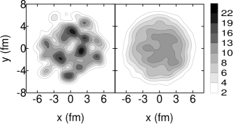
Figure 1: Examples of initial conditions for central Au+Au collisions given by NeXus at mid-rapidity plane. The energy density is plotted in units of GeV/fm³. Left: one random event. Right: average over 30 random events (corresponding to the smooth initial conditions in the usual hydro approach).

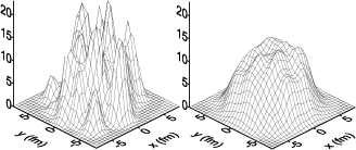
Figure 2: A different representation of the same IC shown in FIG. 1, at mid-rapidity plane. The vertical axis represents the energy density in units of GeV/fm³.

though the number of events is only 30. Similar bumpy event structure was also shown in calculations with HIJING gyulassy . So, the main question here is whether the averages over the observables computed starting from such fluctuating IC, like the one at the left panel of Figs. 1 and 2 are similar or sizeably different from the correspondent ones computed from averaged smooth IC like that at the right panel there, or symbolically,

$$<f>\equiv\frac{1}{N}\sum_{j=1}^{N}(\mbox{IC}\rightarrow f)_{j}\ \simeq \ \frac{1}{N}\sum_{j=1}^{N}(\mbox{IC})_{j}\rightarrow f$$  ? (7)

$$\equiv \ (<IC>\rightarrow f)\,,$$

where $<f>$ is the value of some relevant quantity $f$, obtained by averaging over $N$ total number of events and (IC$\rightarrow f)_{j}$ is the value of the same quantity in the $j$-th event, with some event-dependent IC, whereas $(<IC>\rightarrow f)$ represents the same quantity $f$ given by the average IC. This is a crucial point in data analyses, because the left-hand side is closer to the data point experimentalists obtain, whereas the right-hand side is the quantity usually computed by theorists for that data point, in order to extract properties of the matter formed in nuclear collisions. If the bumpy structure shown by event generators effectively exists in experimental situations, then how do these hot spots manifest themselves in the observables?

A general conclusion one can draw about this question is that the total entropy of the system becomes always smaller when one takes such fluctuations into account, in comparison to the case without fluctuations, which means with average over the event-by-event fluctuating IC taken before the expansion. This can be seen by observing that, in ideal hydrodynamics, both energy and entropy are conserved. Then, considering for simplicity an ideal gas so that $S_{i}=\alpha(E_{i})^{3/4}$, with $\alpha=$const.$>0$, for each random event,

$$<E> = \frac{1}{N}\sum_{i}E_{i}$$ (8)

$$<S> = \frac{1}{N}\sum_{i}S_{i}$$ (9)

$$= \frac{\alpha}{N}\sum_{i}(E_{i})^{3/4}$$

$$= \frac{\alpha}{N}\sum_{i}<E>^{3/4}\left[1+\frac{\Delta E_{i}}{<E>}\right]^{3/4}$$

$$\sim \,\alpha<E>^{3/4}-\frac{3\alpha}{32N}\sum_{i}<E>^{3/4}\left[\frac{\Delta E_{i}}{<E>}\right]^{2}$$

$$< \,\alpha<E>^{3/4}.$$

Here, $<E>$ and $<S>$ in the left-hand sides mean the averaged energy and entropy over the fluctuating events, whereas the right-hand side of $<S>$ is the entropy corresponding to the averaged initial conditions, with the averaged energy $<E>$. The linear terms of the expansion in $\Delta E_{i}/<E>$ are cancelled out when the summation is performed. If one recalls that particle multiplicity is proportional to the entropy for each particle species, one would expect that also the multiplicity becomes, in general, smaller when one takes such fluctuations into account.

Other possible manifestations of this inhomogeneity of IC that we can expect intuitively are: enhancement of high-$p_{T}$ components due to more violent expansion in the surface region, smaller HBT radii, due to concentrations of matter in small spots, azimuthal asymmetry even in central collisions. However, computations are needed to obtain quantitative conclusions, whether such discrepancies are meaningful or not. We shall discuss this question in Sec. VI.

III Equations of state

As mentioned already, the basic assumption in hydrodynamical models is the local thermal equilibrium. Once this condition is satisfied, all the thermodynamical relations should be valid in each space-time point . Thus, the energy, pressure and temperature are given as functions of baryon number and entropy densities, specifying the properties of the matter. In this Section, we discuss how to obtain simple phenomelogical equations of state (EoS) for the hydrodynamical description of relativistic nuclear collisions kodama .

III.1 Hadronic gas

The strong interactions among hadrons are very complicated and difficult to be incorporated into the EoS for practical use. However, for very high energy, we may consider that the hadronic gas may be approximated as an ideal gas, although the degree of approximation can not be evaluated theoretially. The recent thermal model for the description of chemical abundances thermal show that such an approach can reproduce quite well the observed multiplicity ratios of produced hadrons. Here we assume that all the particles can be treated as quantum ideal gas, except for a correction due to the excluded volume. We also include a main part of observed resonances in Particle Data Tables. The inclusion of resonances can be considered as an effective way to consider the interactions among hadrons as explained later.

First, we recall that, in a grand canonical ensemble for an ideal gas of quantum particles, the thermodynamical potential per volume (the pressure) is given by

$$p(T,\mu)=\frac{\theta\,g}{(2\pi)^{3}}\int d^{3}k\ ln(1+\theta\,e^{\beta\left(\mu-\epsilon(k)\right)})$$ (10)

were $\theta$ $=\pm 1$ ($+$ for fermions, $-$ for bosons), $\beta=1/T$ is the inverse of the temperature $T$, $\mu$ the chemical potential, $g$ the degeneracy factor and $\epsilon(k)=\sqrt{k^{2}+m^{2}}$ with $m$ the mass of the particle. The number density $n$ and the energy density $\varepsilon$ can be obtained by the usual thermodynamical relations, $n=(\partial p/\partial\mu)_{V,T}\,$, $\varepsilon=(\partial p/\partial\beta)_{\lambda}\,$, where $\lambda=e^{\beta\mu}$ is the fugacity. The entropy density of the gas can be calculated as $s=\beta(p+\varepsilon-\mu n)$.

For example, in Landau’s model Landau , the equation of state was taken as that of the massless pion gas. For bosons with $m=\mu=0,$ Eq. (10) can be integrated analytically to give

$$p(T)=\frac{g\,\pi^{2}}{90}T^{4},$$ (11)

and accordingly

$$s=\frac{g\,\pi^{2}}{15}T^{3},\ \ \varepsilon=3p=\frac{g\,\pi^{2}}{30}T^{4}.$$ (12)

For the pion gas, due to the isospin factor, we can take $g=3$.

For more realistic equations of state, we should include all the resonance particles in the gas. Furthermore, we should also take into account more than one type of conserved quantum numbers, such as electric charge (equivalently the 3^rd component of isospin), baryon number and strangeness. In this case, the chemical potential must be written as $\mu=B\mu_{B}+S\mu_{S}+T^{\left(3\right)}\mu_{3}$ where $B,S,T^{\left(3\right)}$ are baryon, strangeness and the thrid component of isospin quantum numbers, respectively, and $\mu_{B},\mu_{S}$ and $\mu_{3}$ are the corresponding chemical potentials. Thus, for a mixture of particles with these conserved quantum numbers, Eq. (10) should be generalized to

$$p_{HG}(T,\mu_{B},\mu_{S},\mu_{3})=\sum_{i}p_{i}(T,\mu_{i}),$$ (13)

where the sum refers to the particle species (including resonances) and $\mu_{i}=B_{i}\mu_{B}+S_{i}\mu_{S}+T_{i}^{\left(3\right)}\mu_{3}$ with $B_{i},S_{i},T_{i}^{\left(3\right)}$ are the quantum numbers of the $i$-th particle species. We verify that the baryon number density of the mixture is

$$n_{B} = \left(\frac{\partial p}{\partial\mu_{B}}\right)_{V,T}$$ (14)

$$= \sum_{i}\left(\frac{\partial p_{i}\left(T,\mu_{i}\right)}{\partial\mu_{B}}\right)$$

$$= \sum_{i}B_{i}\ n^{\left(i\right)},$$

where $n^{(i)}=(\partial p_{i}(T,\mu_{i})/\partial\mu_{i})$ is the number density of the $i$-th particle species.

Except for pions, most of hadrons and resonances can be well approximated by the Boltzmann limit. In this case, we have

$$p_{i}(T,\mu_{i})\simeq g_{i}\frac{T^{2}m^{2}}{2\pi^{2}}K_{2}\left(\frac{m_{i}}{T}\right)e^{\mu_{i}/T},$$ (15)

and

$$n_{i}=g_{i}\frac{Tm^{2}}{2\pi^{2}}K_{2}\left(\frac{m_{i}}{T}\right)e^{\mu_{i}/T},$$ (16)

where $K_{2}$ is a modified Bessel function. From these relations, we can see immediately the usual ideal gas relation,

$$p_{i}=n_{i}T\,.$$ (17)

When the widths of the resonances are taken into account, Eq.(13) must be modified. For an interacting gas, the power series expansion of the pressure in terms of fugacity,

$$p(T,\mu)=p^{id}(T,\mu)+T\sum_{n=2}^{\infty}b_{n}(T)e^{\beta\mu n},$$ (18)

is known as the cluster expansion (which is intimately related with the virial expansion) and $b_{n}$ are called “virial” coefficients. Here, $p^{id}$ is the pressure of the corresponding ideal gas and, roughly speaking, the index $n$ in the sum represents the order of multiple particle interactions. For $n=2,$ the contribution to the pressure comes from the 2-body interactions. Beth and Uhlenbeck Beth-Uhlen showed that the second virial coefficient can be expressed in terms of the scattering phase-shift of constituting particles. This approach was generalized to the relativistic Boltzmann gas by Dashen, Ma and Bernstein dashen and the result for $b_{2}$ is

$$b_{2}(T) = \frac{T}{2\pi^{2}}\int_{W_{0}}^{\infty}dW~{}W^{2}K_{2}(\beta W)$$ (19)

$$\times\frac{1}{\pi}\sum_{\ell}(2\ell+1)\frac{\partial}{\partial W}\delta_{\ell}(W)\,,$$

where $\delta_{\ell}(W)$ is the phase shift for the $\ell$-th partial wave.

Consider the case of a gas with mass $M$ and suppose there exists a resonance in the two particle collision,

$$M+M\rightarrow M_{R}\,.$$ (20)

When the resonance has a width $\Gamma$ and spin $J$, only $\ell=J$ dominates the sum and

$$\delta_{\ell}(W)=\frac{\Gamma}{2}\frac{1}{M_{R}-W}\,,$$ (21)

so that we have the Breit-Wigner formula,

$$\frac{\partial}{\partial W}\delta_{\ell}(W)=\frac{\Gamma}{2}\frac{1}{(M_{R}-W)^{2}+\Gamma^{2}/4}\,.$$ (22)

Therefore, the pressure of the system can be written as

$$p=p^{id}+p_{R}\,,$$

where

$$p_{R}=g_{R}\,\frac{T^{2}\Gamma}{4\pi^{3}}e^{\beta\mu_{R}}\int_{W_{0}}^{\infty}dW\frac{W^{2}K_{2}(\beta W)}{(M_{R}-W)^{2}+\Gamma^{2}/4}\ ,$$ (23)

with

$$g_{R} = 2S+1\,,$$

$$\mu_{R} = 2\mu\,.$$

For extremely narrow resonances, $\Gamma\rightarrow 0\,,$

$$p_{R}\rightarrow g_{R}\frac{T^{2}M_{R}^{2}}{2\pi^{2}}K_{2}(\beta M_{R})e^{\beta\mu_{R}},$$ (24)

which is exactly the pressure of the ideal relativistic Boltzmann gas made of resonances with mass $M_{R}\,$. Eq. (23) suggests that, for more general case, the effect of resonance width can be obtained by a convolution of the normalized mass spectrum $f(M)$ of the resonance, with the pressure $p^{id}(M)$ of the ideal gas of mass $M$, as

$$p_{R}=\int dM_{R}f(M_{R})p^{id}(M).$$

III.2 Effect of resonance width as a function of temperature

Equation (23) shows that the effect of the resonance width on the pressure of the gas is temperature dependent. To see this effect, let us introduce the quantity,

$$F(T,M_{R})= \frac{\Gamma}{M_{R}^{2}K_{2}(M_{R}/T)}\hfill$$

$$\times\int_{W_{0}}^{\infty}dW\frac{W^{2}K_{2}(W/T)}{(M_{R}-W)^{2}+\Gamma^{2}/4}\,,$$ (25)

so that

$$p_{R}=p_{R}^{\Gamma=0}\times F(T,M_{R},\Gamma).$$ (26)

Another way to see the effect of the width, we may introduce the effective mass of the resonance $M_{eff}$ defined

Figure 3: Correction factor $F$ as function of temperature $T$ for the resonance $\rho$.

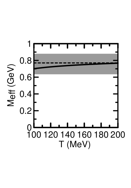
Figure 4: Effective mass of the resonance $\rho$ as function of temperature $T$. The dark area corresponds to the resonance width.

Figure 5: Correction factor $F$ as function of temperature $T$ for the resonance $f$.

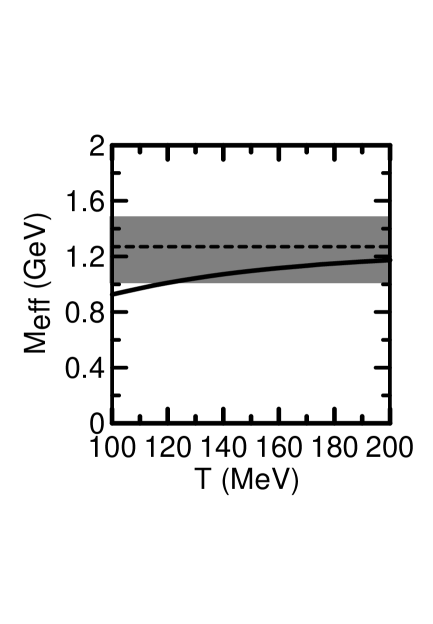
Figure 6: Effective mass of the resonance $f$ as function of temperature $T$. The dark area corresponds to the resonance width.

by

$$M_{eff}^{2}K_{2}(\beta M_{eff})\equiv M_{R}^{2}K_{2}(\beta M_{R})F(T,M_{R}).$$

Using this effective mass, we can write the resonance pressure as

$$p_{R}=g_{R}\frac{T^{2}M_{eff}^{2}}{2\pi^{2}}K_{2}(\beta M_{eff})e^{\beta\mu_{R}},$$ (27)

that is, as if the pressure of ideal particle with mass $M_{eff}$. In Figs. 3,4,5 and 6, we show the temperature dependence of $F$ and $M_{eff}$ for two tipical cases, one for the resonance $\rho$ (light and narrow width) and the resonance $f$ (heavy and large width) resonances. As we see, the ideal gas approximation deviates substancially for low temperature, especially for large width particles. The ideal gas approximation is only valid for $T\gg\Gamma$.

III.3 Excluded-volume correction

From the analysis of thermal modeslthermal , it became clear that the ideal gas description requires a modification to adjust the size of the system. The volume to fit the particle abundances is found to be too small. To avoid this problem, the correction due to the excluded volume effect, like a Van der Waals hard core correction is introduced eos_ev . According to this prescription, Eq. (13) is modified by the following coupled equations

$$p_{HG}(T,\mu_{B},\mu_{S},\mu_{3}) = \sum_{i=1}p_{i}^{id}(T,\tilde{\mu_{i}})\,,$$ (28)

$$\tilde{\mu_{i}} \equiv \mu_{i}-v_{i}\,p_{HG}\,,$$ (29)

where as before $\mu_{i}=B_{i}\mu_{B}+S_{i}\mu_{S}+T_{i}^{3}\mu_{3}$ is the chemical potential and $v_{i}$ is the excluded volume of the $i$-th hadron species. The superscript $id$ refers to the ideal gas case. The above equations constitute an implicit equation for $p_{HG}$ so that these two equations are solved iteratively to obtain $p_{HG}$ for a given set of parameters, $T,\mu_{B},\mu_{S}$ and $\mu_{3}$. The number density of the $i$-th hadron is given by

$$n_{i}^{excl}(T,\mu_{i})=\frac{n_{i}^{id}(T,\tilde{\mu_{i}})}{1+\sum_{j}v_{j}\,n_{j}^{id}(T,\tilde{\mu_{j}})}\,,$$ (30)

where $n_{i}^{id}$ is the ideal gas expression of the particle density for the $i$-th particle species.

III.4 Gas of Quarks and Gluons

The simplest way to introduce the phase of quarks and gluons in the equations of state is the use of the MIT Bag model. The effect of gluon and quark condensate in the physical vacuum is expressed as the enerdy density of the vacuum (or vacuum pressure). Thus the energy density and pressure of an ideal quark-gluon gas calculated in the QCD vacuum should be modified according to the rule,

$$\varepsilon \rightarrow \varepsilon+B,$$

$$p \rightarrow p-B,$$

where $B$ is the vacuum pressure. Note that this vacuum pressure has an analogous property of the cosmological constant $\Lambda$ of Einstein. Now, when we consider just the $u$ and $d$ quarks and neglect their masses, we have

$$p_{qgp} = \frac{g_{q}}{6\pi^{2}}\left[\frac{1}{4}\mu_{q}^{4}+\frac{\pi^{2}}{2}\mu_{q}^{2}T^{2}+\frac{7\pi^{4}T^{4}}{60}\right]$$ (31)

$$+ \frac{g_{G}\pi^{2}}{90}T^{4}-B\,,$$

with

$$g_{q} = 2\times 2\times 3\,,$$

$$g_{G} = 2\times 8\,,$$

the statisfical factors of quarks and gluons. For quarks, we have $\mu_{q}=\mu_{B}/3\,.$ For $\mu_{B}=0\,,$ we have

$$p_{qgp}^{(ud)}=37\times\frac{\pi^{2}}{90}T^{4}-B$$ (32)

or effectively $g_{qgp}=37\,.$ To include the strangeness and also charge conservation, we proceed in the same way as the hadronic gas and we have

$$p_{qgp}(T,\mu_{B},\mu_{S},\mu_{3}) \!=\frac{g_{l}}{6\pi^{2}}\!\left[\frac{1}{4}\mu_{u}^{4}+\frac{\pi^{2}}{2}\mu_{u}^{2}T^{2}\!+\!\frac{7\pi^{4}T^{4}}{60}\right]$$

$$+\frac{g_{l}}{6\pi^{2}}\!\left[\frac{1}{4}\mu_{d}^{4}+\frac{\pi^{2}}{2}\mu_{d}^{2}T^{2}\!+\!\frac{7\pi^{4}T^{4}}{60}\right]$$

$$+p_{s}^{id}(T,\mu_{s})+p_{s}^{id}(T,-\mu_{s})$$

$$+\frac{g_{G}\pi^{2}}{90}T^{4}-B\,,$$ (33)

where $g_{\ell}=2\times 3$ and

$$\mu_{u} =\frac{1}{3}\mu_{B}+\frac{1}{2}\mu_{3}\,,$$

$$\mu_{d} =\frac{1}{3}\mu_{B}-\frac{1}{2}\mu_{3}\,,$$

$$\mu_{s} =\frac{1}{3}\mu_{B}-\mu_{S}\,.$$

III.5 Construction of equations of state for the practical use

The expressions Eqs. (28,29) or Eq. (33) are, however, not convenient for the use in hydrodynamical calculations. This is because the variables in such calculations are the conserved quantum numbers and the entropy density and not the chemical potentials and the temperature. So, we need to invert the relations,

$$n_{B} = n_{B}(T,\mu_{B},\mu_{S},\mu_{3})\,,$$ (34)

$$n_{S} = n_{S}(T,\mu_{B},\mu_{S},\mu_{3})\,,$$ (35)

$$n_{3} = n_{3}(T,\mu_{B},\mu_{S},\mu_{3})\,,$$ (36)

$$s\ \, = s\ \,(T,\mu_{B},\mu_{S},\mu_{3})\,,$$ (37)

to get

$$\mu_{B} = \mu_{B}(n_{B},n_{S},n_{3},s)\,,$$ (38)

$$\mu_{S} = \mu_{S}(n_{B},n_{S},n_{3},s)\,,$$ (39)

$$\mu_{3} = \mu_{3}(n_{B},n_{S},n_{3},s)\,,$$ (40)

$$T\ = T\ (n_{B},n_{S},n_{3},s)\,.$$ (41)

However, this is a formidable task even numerically. We are thus forced to reduce the degrees of freedom for the practical application to hydrodynamics. For this purpose, we set the isospin and strangeness densities to null everywhere. That is, we impose the conditions,

$$n_{S} = 0\,,$$ (42)

$$n_{3} = 0\,.$$ (43)

These conditions together with Eqs. (35) and (36) determine $\mu_{S}$ and $\mu_{3}$ as functions of $T$ and $\mu_{B}\,$. Therefore, $n_{B}$ and $s$ in Eqs. (34) and (37) become now functions of two variables $T$ and $\mu_{B}\,$,

$$n_{B} = n_{B}(T,\mu_{B})\,,$$ (44)

$$s = s(T,\mu_{B})\,,$$ (45)

which can be inverted numerically and give

$$T = T(n_{B},s)\,,$$ (46)

$$\mu_{B} = \mu_{B}(n_{B},s)\,.$$ (47)

The above inversion process allows us to write any of thermodynamcial quantities as functions of $n_{B}$ and $s$, both in hadronic gas and quark-gluon plasma. Then, for a given pair of density parameters $n_{B}$ and $s$, we should determine which phase the physical system assumes. When two phases are in equlibrium, we must have sollf

$$p_{HG}(T,\mu_{B})=p_{QGP}(T,\mu_{B})$$ (48)

so that it determines the phase boundary line in $(\mu_{B},T)$ plane and separates this plane into two domains. The domain where $p_{HG}>p_{QGP}$ is the hadron gas phase and the other $p_{HG}<p_{QGP}$ is the QGP phase. These two domains are in contact on the phase boundary line Eq. (48).

However, the above two domains in $(\mu_{B},T)$ plane are mapped into two separated domains in the $(n_{B},s)$ plane and there appeas a new third domain between them. That is, the phase boundary line $(\mu_{B},T)$ plane spreads into a domain in the $(n_{B},s)$ plane. This domain is the mixed phase. In oder to determine thermodynamical quantities in this mixed phase as functions of $(n_{B},s)$, we should introduce another criterion in addition to the phase boundary condition of Gibbs. As mentioned above, any point $(T,\mu_{b})$ on the phase boundary line corresponds to two points in the $(n_{B},s)$ plane, one for the hadron phase, $(n_{B}^{H},s^{H})$ and other, $(n_{B}^{Q},s^{Q})$ for the QGP phase. In the mixed phase, any density of extensive quantity, should be a linear function of the qgp/hadron concentration ratio. Thus for a given value of the baryon number density $n_{B}$ in the mixed phase, $(n_{B}^{H},s^{H})$ and $(n_{B}^{Q},s^{Q})$ should satisfy

$$s=\frac{s^{Q}-s^{H}}{n_{B}^{Q}-n_{B}^{H}}(n_{B}-n_{B}^{H})+s^{H}.$$ (49)

From this equation, we determine the two points on the phase boundaries, $(n_{B}^{H},s^{H})$ and $(n_{B}^{Q},s^{Q})$. All the other extensive quantities, say $\varepsilon$, can then be obtained as

$$\varepsilon=\frac{\varepsilon^{Q}-\varepsilon^{H}}{n_{B}^{Q}-n_{B}^{H}}(n_{B}-n_{B}^{H})+\varepsilon^{H}.$$ (50)

Finally we can construct the equations of state in the whole region of $(n_{B},s)$. The parameters of the final equations of state are then,

• Number of resonances included in the hadronic gas: Here, we take all the mesons with mass smaller than 1.5 GeV, and baryons smaller than 2 GeV. Resonance widths are not included.

• Quark masses: We may safely take $m_{u}=m_{d}=0$, but for the strange quark, we take $m_{s}=120$ MeV.

• Size of excluded volume: In the example shown in the figures below, $\nu_{0}=(4\pi r_{0}^{3}/3)$ with $r_{0}=0.7$ fm for baryons and $r_{0}=0$ for mesons.

• Bag constant: We take $B=380$ MeV/fm³.

Fig. 7 shows the line of constant temperature in $(n_{B}\,,s)$ plane. Fig. 8 shows the lines of constant entropy per baryon in $(\mu_{B}\,,T)$ plane.

Note that the present equations of state have, by construction, the first order phase transition between hadronic gas and quark gluon plasma. Recent lattice calculations latt indicate that there exists a critical point so

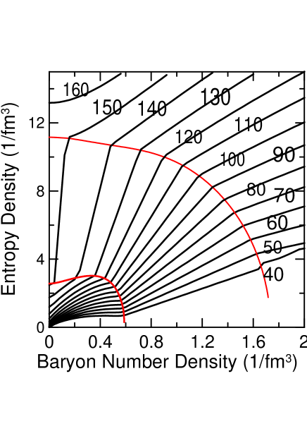
Figure 7: Isotherms in $(n_{B},s)$ plane. Values of the temperatures are indicated in the figure. Hadron gas, mixed phase and quark gluon plasma are clearly seen.

Figure 8: Constant entropy per nucleon curves in the $(\mu,T)$ plane. The numbers indicate $(s/n_{B})$ values.

that the phase transition in the region starting from that point to zero $\mu_{B}$ axis is not the first order but may be either a higher order transition, or a smooth cross over Raj . Effect of such possibilities should be investigated within the hydrodynamical models.

IV Resolution of hydrodynamic equations

In general, exact analytic resolution of relativistic hydrodynamics is a difficult task due to the highly non-linear nature of these equations. So, usually one resorts to numerical computations. However, since the analytical studies are more transparent, it would be useful to find analytical soluions, even though they correspond to highly ideal cases. Khalatnikov’s one-dimensional analytical solution Khalatnikov to Landau’s initial conditions Landau , namely, ideal fluid at rest in a Lorentz contracted thin spatial region, gave rise to a new approach in high-energy physics. The boost-invariant solution scale-invariant found 20 years later, is frequently utilized as the basis for estimations of initial energy densities in ultra-relativistic nucleus-nucleus collisions Bjorken . Below, we shall first describe families of analytical solutions we obtained in collaboration with T. Csörgő tamas1 ; tamas2 .

Considering that it is not trivial to analytically solve the equations of hydrodynamics, it would be nice if we could develop a method to obtain an approximate but analytical solution of hydrodynamics. This has been done with variational formulation variational , although we had not develop it further by applying it to practical problems of high-energy nuclear collisions. However, we did apply the variational method to develop a numerical code SPheRIO, based on the so-called smoothed-particle hydrodynamics (SPH) Lucy ; Monaghan tecnique, to high-energy nuclear collisions sph , which is flexible enough, capable to treat systems with configurations without any symmetry and also exploding in time.

In the following, after presenting some analytical solutions, we shall describe in the subsection IV.2 the variational formulation of hydrodynamics, showing how it could used to get approximate solutions. Then, in the subsection IV.3, we shall apply this method to adapt the SPH hydrodynamics for relativistic heavy-ion collisions.

IV.1 Analytic solutions

After Landau’s initial proposal Landau , the first analytic solution obtained is due to Khalatnikov Khalatnikov , considering 1-dimensional expansion of ideal gas. A more simpler boost-invariant solution has been obtained later scale-invariant and applied to estimate the initial energy densities in ultra-relativistic nucleus-nucleus collisions Bjorken . Both of these have been frequently used in the study of nuclear collisions, showing the usefulness of such simple analytical solutions.

However, the boost-invariant solution has some shortcomings: i) it is scale invariant, having a flat rapidity distribution, corresponding to the extreme relativistic collisions, which has never been seen; ii) it contains no transverse flow. In tamas1 , we tried to overcome these shortcomings. We started by assuming a simple equations of state, corresponding to a gas containing massive conserved quanta, namely,

$$\varepsilon = mn+\kappa p\,,$$ (51)

$$p = nT\,,$$ (52)

having two free parameters, $m$ and $\kappa$. Non-relativistic hydrodynamics of ideal gases corresponds to the limiting case of $m>>T$, ${\mathbf{v}}^{2}<<1$ and $\kappa=3/2\,$.

Then, we looked for similarity flows, i.e.,

$$\mathbf{v} = \left(\frac{\dot{X}(t)}{X(t)}x,\frac{\dot{Y}(t)}{Y(t)}y,\frac{\dot{Z}(t)}{Z(t)}z\right),$$ (53)

$$f(x^{\mu}) = f_{0}\left(\frac{V_{0}}{V}\right)^{a}F(s)\,,$$ (54)

where $X(t),Y(t),Z(t)$ are the scales of length, in three orthogonal directions, and $f(x^{\mu})$ is any of the thermodynamical quantities, such as $n(x^{\mu}),T(x^{\mu}),p(x^{\mu}),\ldots,$ and

$$s=\frac{x^{2}}{X^{2}}+\frac{y^{2}}{Y^{2}}+\frac{z^{2}}{Z^{2}}$$ (55)

is a scaling variable.

Using this parametrization for the one-dimensional expansion, it can be easily verified, by direct substitution into eqs.(1,2) with eqs.(4,51,52,53 and 55), that a family of solutions can be written as

$$v = z/t\equiv\tanh\eta,$$

$$n = n_{0}(t_{0}/\tau){\mathcal{V}}(s),$$

$$p = p_{0}(t_{0}/\tau)^{1+1/\kappa},$$

$$T = T_{0}(t_{0}/\tau)^{1/\kappa}\frac{1}{{\mathcal{V}}(s)},$$ (56)

with $p_{0}=n_{0}T_{0}$ and where ${\mathcal{V}}(s)$ is an arbitrary non-negative function of $s=z^{2}/(\dot{Z}_{0}^{2}t^{2})$. The index $0$ stands for the initial values. Thus, this is a family of one-dimensional similarity flows, but it is not scale invariant and $n$ and $T$ are not constant for a constant $\tau$.

Next, considering cylindrically symmetric flows, with boost invariance along $z$ direction (collision axis), we could find the following family of solutions, for transverse flows:

$${\mathbf{v}} = {\mathbf{r}}/t\,,\quad\mbox{\rm for}\quad|{\bf r}|\leq t,$$

$$n = n_{0}(\tau_{z0}/\tau))^{3}{\mathcal{V}}(s),$$

$$p = p_{0}(\tau_{z0}/\tau)^{3+3/\kappa},$$

$$T = T_{0}(\tau_{z0}/\tau))^{3/\kappa}\frac{1}{{\mathcal{V}}(s)}\,.$$ (57)

Here, $p_{0}=n_{0}T_{0}$ and ${\mathcal{V}}(s)$ is an arbitrary non-negative function of $s$ ($=r_{t}^{2}/(\dot{R}^{2}_{0}\tau_{z}^{2})\,$ in this case), with $r_{t}=\sqrt{x^{2}+y^{2}}\,$ and $\dot{R}_{0}=\sqrt{\dot{X}_{0}^{2}+\dot{Y}_{0}^{2}}\,$ and $\tau_{z}=\sqrt{t^{2}-z^{2}}\,$. So, this is a generalization of the one-dimensional scale-invariant solution, including a class of transverse flows.

More recently tamas2 , we extended these solutions still further, considering less symmetrical flows, but still keeping the same EoS (1,2) and similarity flow, with constant velocity, as it appears in eqs.(56,57).

IV.2 Variational formulation

As shown above, even for very simple equations of state, analytic solutions are limited to special cases. For realistic situations, even the equations of state themselves are available only in the form of numerical tables. Therefore, the numerical resources are essential for realistic studies of hydrodynamical behavior of ultra-relativistic collisional processes. However, it is well-known that any numerical method for partial differencial equations requires highly sophisticated techniques to avoid numerical instabilities, and usually it needs a very large scale computation, especially when we want to describe correctly explosive processes such as relativistic heavy-ion collisions. However, as emphasized in the Introduction, in the hydrodynamic approach of high-energy nuclear collisions, its main ingredients, i.e., the equations of state, the initial conditions and the freezeout conditions are not quite well known. In such a situation, we actually don’t need a very precise solution of the hydrodynamic equations, but a general flow pattern which characterizes the final configuration of the system as a response to given equations of state, initial conditions and the decoupling procedure. So, we prefer a rather simple scheme of solving the hydrodynamic equations, not unnecessarily too precise but robust enough to deal with any kind of geometry. From this point of view, we stressed in Ref. variational the advantage of a variational approach to relativistic hydrodynamics.

Although not commonly found in general textbooks, the variational formulation of hydrodynamics has been studied by several authors Taub+ ; Yourgrau . In Ref. variational , starting from the action

$$I=\int d^{4}x\left\{-\varepsilon\right\},$$ (58)

where $\varepsilon$ is the proper energy density, the relativistic hydrodynamics was derived from the variational principle.

Here, we show its derivation, generalizing to include the rotational flow. To do this, we introduce the two variables, the proper baryon density, $n$, and entropy density, $s$, which satisfy the conservation laws,

$$\partial_{\mu}(nu^{\mu})=0\;,$$

$$\partial_{\mu}(su^{\mu})=0\;.$$ (59)

where $u^{\mu}$ is the four velocity of the field, satisfying the normalization,

$$u^{\mu}u_{\mu}=1\,.$$ (60)

The functional form of the energy density,

$$\varepsilon=\varepsilon\left(n,s\right)$$

specifies the thermodynamical properties of the fluid. The pressure, temperature and chemical potential are obtained by the usual thermodynamic relations,

$$p = n\frac{\partial[\varepsilon(n,s)/n]}{\partial n}\,,$$

$$T = \frac{\partial\varepsilon(n,s)}{\partial s}\quad\quad\quad\mbox{and}$$

$$\mu = \frac{\partial\varepsilon(n,s)}{\partial n}\,.$$

The hydrodynamical equations of motion for the fluid is given by the variational principle with respect to $n$, $s$ and $u^{\mu}$ under constraints, Eq. (59) and the normalization of the four-velocity, Eq.(60). These constraints can be incorporated in the variational principle in terms of Lagrangian multipliers to write

$$\delta\int d^{4}[ - \varepsilon(n,s)+\lambda\partial_{\mu}(nu^{\mu})+\zeta\partial_{\mu}(su^{\mu})$$ (61)

$$- \frac{1}{2}w\left(u^{\mu}u_{\mu}-1\right)]=0\,,$$

where $\lambda,\zeta$ and $w$ are Lagrangian multipliers and arbitrary functions of $x$. Equivalently, the fluid dynamics is given by the effective Lagrangian,

$${\cal L}_{eff}^{(fluid)}(n,s,u^{\mu},\lambda,\zeta,w)=\! - \!\varepsilon(n,s)-nu^{\mu}\partial_{\mu}\lambda$$

$$- \!su^{\mu}\partial_{\mu}\zeta-\frac{w}{2}(u^{\mu}u_{\mu}-1)\,,$$

where now all of $n,s,u^{\mu},\lambda,\zeta,w$ are independent variational variables.

The variations with respect to $n,s$ and $u^{\mu}$ lead immediately to

$$-\mu-u^{\mu}\partial_{\mu}\lambda = 0\,,$$ (63)

$$-T-u^{\mu}\partial_{\mu}\zeta = 0\,,$$ (64)

$$-n\partial_{\mu}\lambda-s\partial_{\mu}\zeta-wu_{\mu} = 0\,.$$ (65)

Variations with respect to $\lambda,\zeta$ and $w$ give simply the constraints, eqs.(59) and (60). Multiplying the both sides of Eq.(65) by $u^{\mu}$, and using eqs.(60,63,64), we get

$$w = n\mu+Ts$$ (66)

$$= \varepsilon+p\,,$$

where $p$ is the pressure. Eq.(66) shows that $w$ is the enthalpy density. Sustiuting back this $w$ into Eq.(65) and multiplying $u_{\nu}$, we have

$$wu_{\mu}u_{\nu}=-(nu_{\nu})(\partial_{\mu}\lambda)-(su_{\nu})(\partial_{\mu}\zeta)\,.$$

Taking the divergence and using the continuity equations $\partial^{\nu}\left(nu_{\nu}\right)=0$ and $\partial^{\nu}(su_{\nu})=0$, we get

$$\partial^{\nu}(wu_{\mu}u_{\nu})=-(nu_{\nu})(\partial^{\nu}\partial_{\mu}\lambda)-(su_{\nu})(\partial^{\nu}\partial_{\mu}\zeta)\,.$$ (67)

But

$$(nu_{\nu})(\partial^{\nu}\partial_{\mu}\lambda) = n\partial_{\mu}(u_{\nu}\partial^{\nu}\lambda)-n(\partial^{\nu}\lambda)(\partial_{\mu}u_{\nu})$$

$$= -n\partial_{\mu}\mu-n(\partial^{\nu}\lambda)(\partial_{\mu}u_{\nu})$$

and analogously

$$(su_{\nu})(\partial^{\nu}\partial_{\mu}\zeta)=-s\partial_{\mu}T-s(\partial^{\nu}\zeta)(\partial_{\mu}u_{\nu})\,,$$

so that Eq.(67) becomes

$$\partial^{\nu}(wu_{\mu}u_{\nu}) = n\partial_{\mu}\mu+s\partial_{\mu}T+(\partial_{\mu}u_{\nu})wu^{\nu}$$ (68)

$$= \partial_{\mu}p+u^{\nu}(\partial_{\mu}u_{\nu})w$$

$$= \partial_{\mu}p\,.$$

Here, we have used Eq.(65) and the Gibbs-Duhem relation,

$$dp=sdT+nd\mu\,,$$ (69)

and the property,

$$u^{\nu}(\partial_{\mu}u_{\nu})=0\,.$$

Finally we arrive at the standard form of the relativistic hydrodynamic equation (1),

$$\partial^{\nu}T_{\mu\nu}=0\,,$$ (70)

where

$$T_{\mu\nu} = wu_{\mu}u_{\nu}-g_{\mu\nu}p$$ (71)

$$= (p+\varepsilon)u_{\mu}u_{\nu}-g_{\mu\nu}p$$

is the usual energy-momentum tensor of the fluid.

It is important to observe that, the effective Lagrangian Eq.(LABEL:L_eff) evaluated in the proper comoving frame of the fluid motion is

$$\left.{\cal L}_{eff}^{(fluid)}\right|_{comoving}=-\varepsilon(n,s)+\mu n+Ts=p\,,$$ (72)

which is nothing but the negative of thermodynamical potential of the system.

Now, interesting application of this approach appears, if we can parametrize possible solutions of continuity equations (59) in terms of a certain number of time-dependent parameters $\vec{a}(t)=\{a_{i}(t),i=1,\ldots,N\}$, such that

$$n = n\left({\bf r},\vec{a}(t),\frac{d\vec{a}(t)}{dt}\right),$$

$$s = s\left({\bf r},\vec{a}(t),\frac{d\vec{a}(t)}{dt}\right),$$

together with the velocity field,

$$u^{\mu}=u^{\mu}\left({\bf r},\vec{a}(t),\frac{d\vec{a}(t)}{dt}\right),$$

then the action, Eq. (58), may be written as a time integral of an effective Lagrangian

$$L_{eff}\left(\vec{a}(t),\frac{d\vec{a}(t)}{dt}\right)=-\int d{\bf r}\;\varepsilon(n,s)\,.$$ (73)

The constraint terms vanish for these ansatz. In this case, the equations of motion for the variables $a_{i}(t)$ are obtained as the Euler-Lagrange equations. This method could be applied to relativistic heavy-ion collisions, trying to describe them in a simple analytic and effective way in terms of few parameters. However, the general parametrization which solve exactly the continuity equations is not easy. An approximate way to solve the continuity equation is proposed in a numerical method called Smoothed Particle Hydrodynamics.

IV.3 Smoothed particle hydrodynamics

The SPH algorithm was first introduced for astrophysical applications Lucy ; Monaghan . In sph , we extended this numerical method to heavy-ion collisions by the use of the variational approach discussed in the preceding subsection.

IV.3.1 SPH representation of densities

The basic idea of the SPH method is to parametrize the continous density distribution of any extensive physical quantity in terms of sum of base functions with finite support. This procedure introduces two types of approximations of different nature. To see this, let us suppose that $A$ is the physical extensive quantity and $a({\bf r},t)$ the corresponding density distribution. We start with the identity,

$$a({\bf r},t)=\int a({\bf r}^{\prime},t)\delta({\bf r-r}^{\prime})d^{3}{\bf r}^{\prime}.$$

Now, let us introduce the first approximation. Substitute the Dirac $\delta$-function by a smooth, normalized function $W$ with finite support, say, $h$, and transform the density $a$ to $\widetilde{a}$ as

$$a({\bf r},t)\rightarrow\widetilde{a}({\bf r},t)=\int a({\bf r}^{\prime},t)W({\bf r-r}^{\prime};h)d^{3}{\bf r}^{\prime},$$ (74)

where as mentioned, $W$ is normalized,

$$\int W({\bf r-r}^{\prime};h)d^{3}{\bf r}^{\prime}=1\,.$$

and having the property of finite support,

$$W({\bf r-r}^{\prime};h)\rightarrow 0,\ {\rm for}\ |{\bf r-r}^{\prime}|>h\,.$$

At this stage, the new density $\widetilde{a}({\bf r},t)$ describes the smoothed part of the original density $a({\bf r},t)$. From the Fourier transform, we can see that for this smoothed density, the Fourier components with large wave numbers, corresponding to

$$k>\frac{1}{h}\ ,$$

vanish rapidly. In other words, the kernel function $W$ serves as the short wavelength cut-off filter. Physically, it is useful to introduce such a filter, since we very often want to eliminate very short scale part in order to extract the global feature of the dynamics of the system. In 60’s, similar idea has been used to smooth out the spectrum density of the nuclear shell model to extract the collective liquid drop potential by Strutinski Strutinski .

Now, we introduce the second approximation. This is rather to do with the practical aspect, that is, to reduce the degee of freedoms envolved in the calculation. We replace the integral Eq.(74) by a finite sum over finite discrete set of points,$\{{\bf r}_{i},\ i=1,..,N\}$.

$$\widetilde{a}({\bf r},t)\rightarrow a_{SPH}({\bf r},t)=\sum_{i}^{N}A_{i}W({\bf r-r}_{i};h),$$ (75)

where the weight $A_{i}$ should be chosen appropriately to minimize the difference between $\widetilde{a}({\bf r},t)$ and $a_{SPH}({\bf r},t)$ everywhere. The above expression means that we are representing the continous density as sum of finite number of unit distributions (kernel) carrying the quantity $A_{i}$. These unit density distributions are centered at the position ${\bf r}_{i}\,$.

Finally, the correspondence,

$$a({\bf r},t)\rightarrow a_{SPH}({\bf r},t)=\sum_{i}^{N}A_{i}W({\bf r-r}_{i};h)$$ (76)

can be considered as an approximation ansatz for the density $a({\bf r},t)$ with finite number of parameters, $\{A_{i},{\bf r}_{i},i=1..,N\}\,$. Due to the normalization of the kernel $W$, we have

$$\int a_{SPH}({\bf r},t)d^{3}{\bf r}=\sum_{i}^{N}A_{i}\,,$$

so that we should choose

$$\sum_{i}^{N}A_{i}$$

as the total value of the quantity $A$ of the system.

IV.3.2 Solution of continuity equations

For the application in Hydrodynamics, we can use these parameters as the variational variables so that they are depending on time. When we deal with one or more extensive quantities, we usually choose one conserved quantity as the reference density, say $\rho$, and represents it by the SPH form, choosing appropriately the weights $\{\nu_{i}\}$ to get

$$\rho_{SHP}({\bf r},t)=\sum_{i}^{N}\nu_{i}W({\bf r-r}_{i}(t);h)\,,$$ (77)

and take ${\bf\nu}_{i}$ constant in time. Other extensive quantity, say $A$, is calculated as in Eq.(76) with weights,

$$A_{i}=\left(\frac{a}{\rho}\right)_{i}\nu_{i}\ .$$ (78)

The quantity $(a/\rho)_{i}$ then represents the quantity $A$ for the unit reference quantity $\rho$ at the position ${\bf r=r}_{i}(t)\,$. Note that the time dependence of the density in Eq.(77) comes from those of $\{{\bf r}_{i}(t)\}\,$. In this sense, Eq.(77) can be understood as if $\{{\bf r}_{i}(t)\}$ are Lagrangian coordinates attached to small volumes of the order of $h^{3},$ with some conserved quantity, such as baryon number or entropy in the adiabatic expansion. From now on, we refer to these unit density distributions characterized by their coordinates $\{{\bf r}_{i}\}$ as “SPH particles”. From Eq.(78), the quantity $A_{i}$ can be interpreted as the part of $A$ carried by the SPH particle $i$.

The most powerful point of the above scheme of SPH representation is that we can solve the continuity equation in a very simple manner. Suppose $M$ is a conserved quantity. Then the corresponding density $\rho$ should satisfy the continuity equation,

$$\frac{\partial\rho({\bf r},t)}{\partial t}+\nabla\cdot(\rho{\bf v})=0\,,$$ (79)

where v is the velocity field. The SPH expression for the current ${\bf j}=\rho{\bf v}$ is

$${\bf j}_{SPH}({\bf r},t)=\sum_{i}{\bf v}_{i}\,\nu_{i}W({\bf r-r}_{i}(t))\,,$$

so that

$$\nabla\cdot{\bf j}_{SPH}({\bf r},t)=\sum_{i}{\bf v}_{i}\,\nu_{i}\nabla W({\bf r-r}_{i})\,.$$

On the other hand, from Eq.(77),

$$\frac{\partial\rho_{SPH}({\bf r},t)}{\partial t} = \sum_{i}\nu_{i}\frac{d}{dt}W({\bf r-r}_{i}(t))$$

$$= \sum_{i}\nu_{i}\frac{d{\bf r}_{i}(t)}{dt}\cdot\nabla W({\bf r-r}_{i}(t))\,,$$

By inspection, if we identify

$${\bf v}_{i}=\frac{d{\bf r}_{i}(t)}{dt}\,,$$

then we can see that Eq.(79) is automatically satisfied.

For the application to the relativistic heavy ion collisions, we can take the entropy and baryon number as the basic conserved quantities. Then, their densities (in the space-fixed frame) are parametrized as

$$s^{\ast}({\bf r},t) = \sum_{i}^{N}\nu_{i}~{}W({\bf r}-{\bf r}_{\,i}(t))~{},$$ (80)

$$n^{\ast}({\bf r},t) = \sum_{i}^{N}b_{i}~{}W({\bf r}-{\bf r}_{\,i}(t))~{},$$ (81)

where $\nu_{i}$ and $b_{9}$ are the entropy and baryon number attached to the $i$-th “particle”. The total entropy and baryon number are then given by

$$S = \int\!d^{3}{\bf r}~{}s^{\ast}({\bf r},t)=\sum_{i}^{N}\nu_{i}~{}.$$ (82)

$$B = \int\!d^{3}{\bf r}~{}n^{\ast}({\bf r},t)=\sum_{i}^{N}b_{i}~{}.$$ (83)

The proper densities of entropy and baryon number are related with these space-fixed frame quantities as

$$s = \gamma^{-1}s^{\ast},$$

$$n = \gamma^{-1}n^{\ast},$$

where $\gamma=u^{0}$ is the Lorentz factor asscociated with the fluid velocity. For the hydrodynamical description of nuclear and hadronic collisions at ultra-relativistic energies, we prefer to use the entropy than the baryon number as the reference conserved number to write the SPH representation of any other extensive quantities. This is because, the baryon number may become zero but the entropy density never vanishes in the physically interesting region within a hydrodynamical description.

IV.3.3 SPH action and SPH equations

In the variational derivation of this method, the set of time-dependent variables $\{{\bf r}_{i},i=1,...,n\}$ are taken as the variational degrees of freedom and their equations of motion are determined by minimizing the action for the hydrodynamic system. Thus, SPH may be considered as an effective description, in which the coordinates $\{{\bf r}_{i}(t)\}$ associated with “particles” are the optimal dynamical parameters which minimize the model action. We observe that $\{\nu_{i}\}$ or $\{b_{i}\}$ are not dynamical variables and are determined by the initital conditions together with the constraints for the variational procedure.

The effective Lagrangian, Eq. (73), is rewritten in SPH representation as

$$L_{SPH}(\{{\bf r}_{i},{\bf{\dot{r}}}_{i}\})=-\sum_{i}\nu_{i}(\varepsilon/s^{\ast})_{i}=-\sum_{i}\left(\frac{E}{\gamma}\right)_{i},$$ (84)

where $E_{i}$ is the “rest energy” of the $i$-th “particle”. Then, the equations of motion are obtained from the usual variational procedure. This leads to the following coupled equations

$$\frac{d}{dt}\left(\nu_{i}\frac{p_{i}+\varepsilon_{i}}{s_{i}}\,\gamma_{i}\,{\bf v}_{i}\right)\hskip 128.0374pt$$

$$\hskip 14.22636pt+\sum_{j}\nu_{i}\nu_{j}\bigg{[}\frac{p_{i}}{{s_{i}^{\ast}}^{2}}+\frac{p_{j}}{{s_{j}^{\ast}}^{2}}\bigg{]}\,{\bf\nabla}_{i}W({\bf r}_{\,i}-{\bf r}_{\,j};h)=0\,.$$ (85)

IV.3.4 General coordinate system

The variational procedure can readily be extended to coordinate systems with a non-Cartesian metric. The use of generalized coordinate systems is particularly important when we consider realistic initial conditions for simulations of RHIC processes. As we know, in a relativistic heavy-ion collisional process, the initial state is a cold, quantum nuclear matter. Just after the collision, the hadronic matter stays at a highly off-shell state and the materialization occurs only after $\sim 1\,$fm/c in the proper time. Therefore, the local thermodynamical state would emerge for some local proper time and not for the global space-fixed time $t$. Thus, it is important to choose a convenient coordinate system for the description of the relativistic heavy-ion collisions. For example, one often uses the hyperbolic time and longitudinal coordinates to be described later.

Let us consider a general coordinate system,

$$ds^{2}=g_{\mu\nu}dx^{\mu}dx^{\nu}.$$ (86)

However, in order to unambiguously define the conserved quantity, we consider only the case that the time-like coordinate is orthogonal to the space-like coordinates,

$$g_{\mu 0}=0\,.$$ (87)

The action principle for the relativistic fluid motion can be written as variational

$$\delta I=-\delta\int d^{4}x\sqrt{-g}\,\varepsilon=0\,,$$ (88)

together with the constraint for the conserved entropy current,

$$(su^{\mu})_{;\mu}=\frac{1}{\sqrt{-g}}\partial_{\mu}(\sqrt{-g}\,su^{\mu})=0\,,$$ (89)

or

$$\frac{1}{\sqrt{-g}}\partial_{\tau}\left(\sqrt{-g}s\gamma\right)+\frac{1}{\sqrt{-g}}\sum_{i}\partial_{i}\left(\sqrt{-g}s\gamma v^{i}\right)=0\,,$$ (90)

where

$$v^{i}=\frac{u^{i}}{u^{0}}$$ (91)

and we use the notation,

$$\tau=x^{0},\,\;\gamma=u^{0}.$$

The generalized gamma factor $\gamma$ is related to the velocity $\vec{v}_{a}$ through $u_{\mu}u^{\mu}=1$, so that

$$\gamma=\frac{1}{\sqrt{g_{00}-\vec{v}^{\,T}\mathbf{g}\,\vec{v}}}\,,$$ (92)

where $-\mathbf{g}$ is the $3\times 3$ space part of the metric tensor. That is

$$\left(g_{\mu\nu}\right)=\left(\begin{array}[]{cc}g_{00}&0\\ 0&-\mathbf{g}\end{array}\right).$$ (93)

Let us now introduce the SPH representation. We may, for example, express the entropy density by the ansatz

$$\sqrt{-g}s\gamma=s^{\ast}\ \rightarrow\ s_{SPH}^{\ast}=\sum_{i}\nu_{i}W(\vec{r}-\vec{r}_{i}(\tau))\,,$$ (94)

or by

$$s\gamma=s^{\ast}\ \rightarrow s_{SPH}^{\ast}=\sum_{i}\nu_{i}W(\vec{r}-\vec{r}_{i}(\tau))$$ (95)

as well. These two possibilities, besides others, are simply different ways to parametrize the variational ansatz in terms of a linear combination of given functions $W(\vec{r}-\vec{r}_{a}(\tau))$. The most important property of an ansatz should be that $W$ satisfies the normalization condition imposed by the basic conserved quantity. Since the total entropy is expressed as

$$S=\int d^{3}\vec{r}\sqrt{-g}\,s\gamma=\sum_{i}\nu_{i}\,,$$ (96)

the normalization of $W$ should be taken to be

$$\int d^{3}\vec{r}\,W(\vec{r}-\vec{r}\,^{\prime})=1\,,$$ (97)

for the parametrization Eq.(94) and

$$\int d^{3}\vec{r}\sqrt{-g}W(\vec{r}-\vec{r}\,^{\prime})=1\,,$$ (98)

for the parametrization Eq.(95). In the usual SPH calculations, it is not desirable to introduce in $W$ the space-time dependence through its normalization condition. In this respect, the most natural way to introduce the SPH representation is Eq.(94). With this choice, the SPH action is given by

$$I_{SPH} = -\int d\tau\int d^{3}\vec{x}\sum_{i}\nu_{i}\left(\frac{\sqrt{-g}\,\varepsilon}{\sqrt{-g}\,s\gamma}\right)_{i}W(\vec{r}-\vec{r}_{i}(\tau))$$ (99)

$$= -\int d\tau\sum_{i}\nu_{i}\left(\frac{\varepsilon}{s\gamma}\right)_{i}.$$

The variational principle leads to the following equation of motion,

$$\frac{d}{d\tau}\vec{\pi}_{i}= - \sum_{j}\nu_{i}\nu_{j}\left[\frac{1}{\sqrt{-g_{i}}\gamma_{i}^{2}}\frac{p_{i}}{s_{i}^{2}}+\frac{1}{\sqrt{-g_{j}}\gamma_{j}^{2}}\frac{p_{j}}{s_{j}^{2}}\right]\nabla_{i}W_{ij}$$ (100)

$$+ \frac{\nu_{i}}{\gamma_{i}}\frac{p_{i}}{s_{i}}\left(\frac{1}{\sqrt{-g}}\nabla\sqrt{-g}\right)_{i}$$

$$+ \frac{\nu_{i}}{2}\gamma_{i}\left(\frac{p+\varepsilon}{s}\right)_{i}(\nabla g_{00}-\vec{v}_{i}^{\,T}\nabla\mathbf{g}\vec{v}_{i})_{i}\,,$$

where

$$\vec{\pi}_{i}=\gamma_{i}\,\nu_{i}\left(\frac{p+\varepsilon}{s}\right)_{i}\mathbf{g}\,\vec{v}_{i}$$ (101)

and the operator $\nabla$ is just the simple derivative operator with respect to the coordinate variable in use.

For ultrarelativistic heavy-ion collisions, a useful set of variables is

$$\tau = \sqrt{t^{2}-z^{2}},$$ (102)

$$\eta = \frac{1}{2}\ln\frac{t+z}{t-z}\,,$$ (103)

$$\vec{r}_{T} = \left(\begin{array}[]{c}x\\ y\end{array}\right).$$ (106)

As mentioned above, the initial conditions for RHIC processes are specified in terms of the proper time rather than of the coordinate time $t$. The variable $\tau$ is not exactly the physical proper time of the matter, but for the initial times it may approximate the proper time.

The metric tensor for this coordinate system is given by

$$g_{00} = 1,$$

$$\mathbf{g} = \left(\begin{array}[]{ccc}1&0&0\\ 0&1&0\\ 0&0&\tau^{2}\end{array}\right),$$

$$\sqrt{-g} = \tau\,.$$

Since the metric is space independent, we can use the parametrization

$$\tau\gamma_{i}s_{i}=s_{i}^{\ast}=\sum_{j=1}^{n}\nu_{j}W(q_{ij}),$$

where

$$q_{ij}=\sqrt{(x_{i}-x_{j})^{2}+(y_{i}-y_{j})^{2}+\tau^{2}(\eta_{i}-\eta_{j})^{2}}$$

and $W$ is normalized as

$$4\pi\int_{0}^{\infty}q^{2}dq\;W(q)=1\,.$$

The SPH equation becomes

$$\frac{d}{d\tau}\vec{\pi}_{i}=-\frac{1}{\tau}\sum_{j}\nu_{i}\nu_{j}\left[\frac{1}{\gamma_{i}^{2}}\frac{p_{i}}{s_{i}^{2}}+\frac{1}{\gamma_{j}^{2}}\frac{p_{j}}{s_{j}^{2}}\right]\nabla_{i}W_{ij}\,,$$

where the $\eta$ component of the momentum is related to the velocity $d\eta/d\tau$ as

$$\pi_{\eta}=\tau^{2}\nu\gamma\left(\frac{p+\varepsilon}{s}\right)\frac{d\eta}{d\tau},$$

whereas in the transverse direction, we have

$$\vec{\pi}_{T}=\nu\gamma\left(\frac{p+\varepsilon}{s}\right)\frac{d\vec{r}_{T}}{d\tau}.$$

The Lorentz factor is given by

$$\gamma=\frac{1}{\sqrt{1-\vec{v}_{T}^{2}-\tau^{2}v_{\eta}^{2}}}.$$

IV.3.5 Landau Model

In order to show the efficiency of the method and also to show the corrrect choice of the coordinate system, let us investigate the Landau model in the SPH scheme, using the ordinaly Cartesian coodinates and $\eta-\tau$ coodinates. Since the analytical solution is known, we can compare the numerical solutions to it.

Figure 9: $a)$ (above) Entropy profiles of the Landau model in Cartesian coordinate for different times. The exact results are given by the broken curves. The SPH solution is shown by the full curves. $b)$ (below) Temperature profiles of the Landau model in the hyperbolic coordinate system (see text), for different time $\tau$. The SPH calculation is represented by the circles, and the exact result by the broken curves.

We thus solve the hydrodynamical evolution of a system of one-dimensional relativistic massless baryon-free gas initially at rest. The equation of state of a relativistic massless boson gas is

$$p=\frac{1}{3}\varepsilon=Cs^{4/3},$$

where

$$C=\left(\frac{15}{128\pi^{2}}\right)^{1/3}.$$

To apply the SPH method, we introduce the discrete one-dimensional space variable ${x_{i}(t),i=1,..,n}$ (and similarly for $\eta-\tau$ coodinates). The relation between the momentum and velocity is then

$$\pi=4C\nu s^{\ast 1/3}\gamma^{2/3}v,$$ (108)

where, in this case, $v$ can be solved analytically with respect to $\pi$.

In Figs. 9$\,a$ and $b$, we show the results of our SPH calculation together with the exact solution Landau . In these examples, we took only $100$ particles with equally spaced $x_{i}$ (or ${\eta_{i}}$). As we see from this example, in spite of rather small number of particles, the SPH solution is quite satisfactory. In particular, when we use the $\eta-\tau$ coordinates with an appropriate distribution of $\nu_{i}^{\prime}s$ (Fig. 9$\,b$), an excellent agreement with the analytical solution can be obtained. The computation time needed to get these solutions is even less than that needed to numerically evaluate the analytical solution.

IV.3.6 Transverse expansion on longitudinal scaling expansion

As a further test, closer to a realistic situation than that of Figs. 9, we calculated the transverse expansion of a cylindrically symmetric homogeneous massless pion gas, undergoing a longitudinal scaling expansion, and ini-

Figure 10: Temperature profile of a cilyndrically symmetric flow with longitudinally scaling expansion, shown as a function of $r=\sqrt{x^{2}+y^{2}}$. The SPH results at $\eta=0$ (circles) are compared with the numerical solution obtained by a space-fixed grid method. The SPH calculation has been perfomed in full 3D.

tially at rest in transverse directions. Such a problem has been discussed by several authors as a useful base to understand the transverse expansion. In Fig. 10, we compare our results (a full $3D$ calculation without assuming cylindrical symmetry) with (2+1) numerical results, obtained by the use of the method of characteristics Pottag . In this example, we used also $50\times 50\times 50$ particles. The result is quite satisfactory. If we decrease the accuracy by $10\%$, we can reduce the particle number almost by one order of magnitude.

IV.3.7 Shock formation and Neumann-Richtmeyer pseudo viscosity

As seen in the previous examples, our entropy-based relativistic SPH method works quite well for the adiabatic dynamics of the massless pion gas. However, for the application to realistic problems, it is fundamental to see how this scheme works for non-adiabatic cases, too. This is because, whenever a piece of fluid matter flows into another region of the fluid with a speed exceeding the sound velocity of the fluid, there appears a shock wave, and this is essencially a nonadiabatic process. Thus, except for a really quasi-static dynamics, there should be an entropy production mechanism. This becomes especially important in a domain close to the phase transition region, because there the velocity of sound tends to zero. In the following, we study some examples of one dimensional shock problems in the scheme of the SPH methods.

The shock front manifests as a discontinuity in thermodynamical quantities in a hydrodynamic solution. Mathematically speaking, the shock front should be treated as a boundary connecting two distinct hydrodynamic solutions. The smoothed particle ansatz excludes such a possibility from the beginning. Since short-wavelength excitation modes do not exist in the SPH ansatz, the energy and momentum conservation required by the hydrodynamics results in very rapidly oscillating motion of each SPH particle. Such a situation occurs, for example, when a very high-energy density gas is released into a low density region. This kind of shock, for the case of a baryon gas, is discussed in Maruhn and also, in the SPH context, in Siegler . Here, we appliy our entropy-based SPH approach to the massless pion gas.

Fig. 11 gives the typical behavior of SPH solution for such a situation, if entropy production is not taken into account. As discussed above, there appear in fact rapid oscillations in thermodynamical quantities just behind the shock front. Actually, such oscillations always appear in any numerical approach if entropy production is not included.

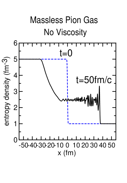
Figure 11: Shock wave formation in one-dimensional pion gas, calculated with SPH. No viscosity is used.

In order to avoid these unphysical oscillations, von Neuman and Richtmeyer Neuman introduced the concept of pseudoviscosity. The idea is to set the dissipative pressure where the shock wave discontinuity is present. To do this, Neuman and Richtmeyer proposed to replace the pressure by

$$p\rightarrow p+Q,$$

where $Q$ is the pseudoviscosity and they took the following ansatz,

$$Q=\left\{\begin{array}[]{ccc}(\alpha\Delta x)^{2}\rho\;(\dot{\rho}/\rho)^{2},&&\dot{\rho}>0\\ 0\,,&&\;\dot{\rho}<0\end{array}\right..$$

The above formula is for nonrelativistic one-dimensional hydrodynamics. Here, $\rho$ is the mass density, $\Delta x$ is the space grid size and $\alpha$ is a constant of the order of unity. In order to generalize the above pseudoviscosity for relativistic SPH case, we replace the quantity $\dot{\rho}/\rho\,$ by $-\theta=-\partial_{\mu}u^{\mu}$ and $\Delta x$ by $h$, where $h$ is as before the width of the smoothing kernel $W$. More precisely, we take the following form which is a slightly modified expression suggested by Ref. Siegler ,

$$Q=\left\{\begin{array}[]{ccc}p\left[-\alpha h\theta+\beta(h\theta)^{2}\right]\,,&&\theta<0\,,\\ 0\,,&&\theta\geq 0\,.\end{array}\right.$$ (109)

where

$$\theta =\frac{1}{V}\frac{dV}{dt}$$

$$=\partial_{\mu}u^{\mu}.$$ (110)

Actually, $Q$ is equivalent to the bulk viscosity and therefore there is no heat flow associated with it. What this artificial viscosity does is to convert the collective flow energy into the microscopic thermal energy. As a consequence, the total energy, that is, the sum of the collective flow energy and the internal thermal energy is still conserved. In order to incorporate the internal energy conservation in the SPH scheme, we substitute all the pressure $p_{i}$ by $p_{i}+Q_{i},$ and we add the following equation for the entropy production,

$$\frac{1}{\nu_{i}}\frac{d\nu_{i}}{dt}=-\frac{Q_{i}\gamma_{i}}{Ts_{i}^{\ast}}\theta_{i}.$$ (111)

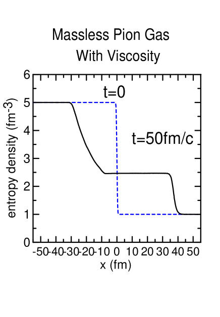
Figure 12: After the introduction of the $Q$ term in the SPH calculation.

Fig. 12 is the solution of the same problem as in Fig. 11, but with the entropy production taken into account. In this calculation, the parameters have been chosen as

$$\alpha=2,\;\beta=4$$

and $h=0.5fm$ for 1000 SPH particles. As we see, the rapid oscillations have been smoothed out (and in turn, the numerical calculation became much more efficient).

It is known that the energy- and momentum-flux conservations through a sock front relate the ratio $s_{2}/s_{1}$ of entropy densities after and before the shock to the velocity $v_{s}$ of the shock front as (Hugoniot-Rankine relation)

$$\frac{s_{2}}{s_{1}}=\frac{2}{3^{3/4}}v_{s}\frac{(9v_{s}^{2}-1)^{1/4}}{(1-v_{s}^{2})^{5/4}}\,.$$ (112)

In Fig. 13, we show the velocity of the shock front obtained in our SPH calculations as function of the entropy ratio(dots). Each point corresponds to the different initial condition. They are compared with the Hugoniot-Rankine relation Eq. (112) (curve). The accordance shows that our SPH calculation reproduces faithfully the conservation of kinetic energy and momentum of the flow through the shock front.

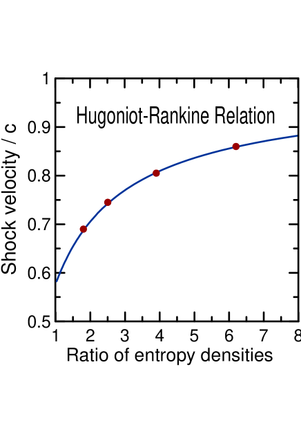
Figure 13: Test of Hugoniot-Rankine relation. The circles are results of SPH calculations with different initial conditions, and the full curve is Eq. (112).

In the usual hydrodynamic computations using space grids, the symmetry of the problem is often a crucial factor to perform a calculation of reasonable size. The SPH method cures this aspect and furnishes a robust algorithm particularly appropriate to the description of processes where rapid expansions of the fluid should be treated. The equations of motion are derived by a variational procedure from the SPH model action with respect to the Lagrangian comoving coordinates. This guarantees that the method furnishes the maximal efficiency for a given number of degrees of freedom, keeping strictly the energy and momentum conservation. For this reason, solutions can be obtained with a very reasonable precision, with a relatively small number of SPH particles. This is the basic advantage of the present method, when we analyze the event-by-event dynamics of the relativistic heavy-ion collisions.

On the other hand, the precision of this method increases rather slowly with the number of SPH particles. Therefore, a relatively large number of particles is required if one wants a very precise numerical solution. However, for the application to the RHIC physics, we may need rather crude precision especially if we consider the dubious validity of the rigorous hydrodynamics. For a calculation with typically $10\%$ errors, the SPH algorithm presented here furnishes a very efficient tool to study the flow phenomena in the RHIC physics.

A fundamental difficulty of the relativistic hydrodynamics for viscous fluid Israel ; Hiscock is that the dissipation term causes an intrinsic instability to the system. This instability basically comes from the fact that the dissipation term contains $\theta=\partial^{\mu}u_{\mu}$ (see Eqs. (109,111)), so that it necessarily introduces the third time-derivative into the equation. This means that we have to specify, at least, a part of the acceleration as the initial condition. Even we specify the initial acceleration, the requirement of the internal self-consistency among the equations above leads to intrinsically unstable solutions. Israel proposed Israel ; Hiscock to cure these difficulties by introducing higher-order thermodynamics with respect to deviations from the equilibrium. Recently this “second order thermodynamics” formalism was discussed in the context of Bjorken type solution Muronga . In the examples presented in the present paper, we did not address this question and simply estimated the quantity $\theta$ from the quantities one time step before. In practice, this will cause no numerical instability and the behavior of the solution is quite satisfactory.

In spite of the above conceptual difficulties when nonadiabatic process is involved, the SPH approach has a nice feature as its flexibility, allowing the treatment of problems with initial conditions without any symmetry, as happens in small systems as those resulting in relativistic nuclear collisions. It should be stressed that, due to the use of Lagrangian coordinates, the method is most suitable for explosive processes like the relativistic heavy ion collisions. (Lagrangian coordinates have been used for treatment of relativistic nuclear collisions also by Nonaka, Honda and Muroya nonaka ). Furthermore, the variatioal approach guarantees that the SPH equations (85) give the optimal description of motions for a given total number of “particles” $\{{\bf r}_{i}(t)\}$, which are our parameters. In this approach, no numerical instabilities will occur, since the whole system is a Lagrangian system. A numerical code, called SPheRIO has been developped by us on the basis of this algorithm. We shall discuss, in Sec.VI, some results obtained using this code.

V Decoupling criteria

V.1 Cooper-Frye prescription

As mentioned in the Introduction, the decoupling process is customarily described using the Cooper-Frye prescription C-F , which gives the invariant momentum distribution as

$$E\frac{d^{3}N}{dp^{3}}=\int_{\sigma}d\sigma_{\mu}p^{\mu}f(x,p)\,.$$ (113)

This description of decoupling introduces a sharp freezeout hypersurface $\sigma\,$, usually characterized by a constant temperature $T_{f.o.}\,$. Before crossing it, particles have a hydrodynamical behavior and, when they cross it suddenly decouple, free-streaming toward the detectors, keeping memory of the conditions (flow, temperature) of where and when they crossed the three dimensional surface.

In SPH representation, we write

$$E\frac{d^{3}N}{dp^{3}}=\sum_{j}\frac{\nu_{j}n_{j\mu}p^{\mu}}{s_{j}|n_{j\mu}u_{j}^{\mu}|}\;f(u_{j\mu}p^{\mu})\,,$$ (114)

where the summation is over all the SPH particles, which should be taken where they cross the hyper-surface $T=T_{f.o.}\,$ and $n_{j\mu}$ is the normal to this hyper-surface.

Another often used procedure is to take such a freezeout temperature not only constant for a given energy but also energy-independent.

Though operationally simple, and actually useful for obtaining a nice comprehension of several aspects of the phenomena, such a concept of sharp freezeout hypersurface and also of a constant freezeout temperature are clearly highly idealized when applied to finite-volume and finite-lifetime systems as those formed in high-energy heavy-ion collisions.

V.2 Finite-size effect

Before going further, let us for a moment assume that such a freezeout temperature is meaningful. At least, as an average temperature, it should exist. Then, how can we estimate it based on the properties of the system? A simple and natural criterion has already been given by Landau Landau , by which a particle decouples when its mean free-path $\ell$ in the medium becomes larger than the system size $L$,

$$\ell>L\,.$$ (115)

This means that $T_{f.o.}\,$ is not an intrinsic thermodynamic property of the fluid, but it depends also on the size of the system. In fernando , we applied this idea to estimate $T_{f.o.}\,$ as function of the incident energy both for $pp$ ($\bar{p}p$) and nucleus-nucleus collisions, obtaining approximately

$$T_{f.o.}\sim(\sqrt{s})^{-1/12}.$$ (116)

Here, the energy dependence appears as a consequence of the increase in the initial energy density, which implies longer expansion time, so larger size $L$ of the system (both longitudinally and tranversally) at the moment of decoupling, requiring lower density, so lower decoupling temperature, too. Figure 14 shows the comparison made in fernando of an estimate of the incident-energy dependence of $T_{f.o.}\,$, using Landau’s criterion mentioned above, with $T_{f.o.}$ obtained in a data analysis of $\pi$ and $K$ transverse-momentum spectra in $pp$ (and $\bar{p}p$) collisions, in terms of a hydrodynamic parametrization of transverse velocity distribution and temperature. The data were taken from ISR ; collider ; Fermilab .

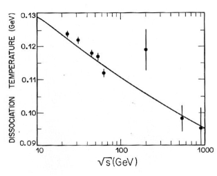
Figure 14: Energy dependence of $T_{f.o.}$ in $pp$ (and $\bar{p}p$) collisions. The solid line is the estimate as explained in the text. The points were obtained from a data analysis fernando .

An independent estimate of $T_{f.o.}(s)$ for $pp$ was made by Navarra et al. udo , based on somewhat different but related freeze-out criterion

$$\tau_{hydro}\sim\tau_{col}\,,$$

where $\tau_{hydro}$ and $\tau_{col}$ are, respectively, characteristic time for hydrodynamic expansion and particle collision, obtaining a similar result.

When Au + Au collisions data began to appear, Xu and Kaneta Nu reported that $T_{f.o.}$ seems to decrease with $\sqrt{s}$ also in nuclear collisions at high energies, and we could verify that the reported results are consistent with $T_{f.o.}\sim(\sqrt{s})^{-1/12}$. It is interesting that, more recently eff-t , in trying to understand the experimentally

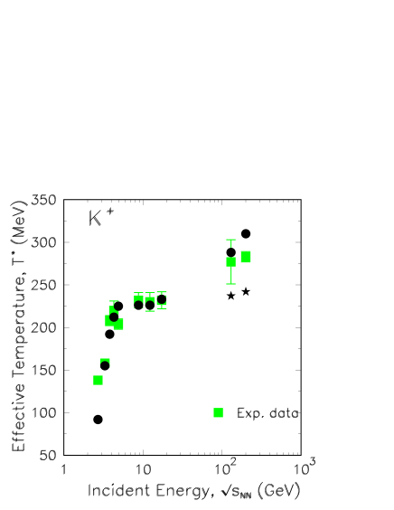
Figure 15: Energy dependence of the inverse slope parameter for $K^{+}$ in central Pb + Pb (Au + Au) collisions. Here, averaged IC were used. Stars correspond to $T_{fo}$=155 MeV (see Table 1). Data are from k_slope

.

Table 1: Freezeout temperature $T_{fo}\,$, averaged transverse velocity $\bar{v}_{T}$ in $-0.5\leq y\leq 0.5$ and the inverse slope parameter $T^{*}$ for $K^{+}$ production in central Pb + Pb (Au + Au) collisions, obtained using SPheRIO with averaged NeXuS IC. $T_{0}$ and $\varepsilon_{0}$ are the initial values at the midpoint of the fluid.

$\sqrt{s}$	$T_{0}$	$\varepsilon_{0}$	$T_{fo}$	$\bar{v}_{T}$	$T^{*}$
(A$\cdot$GeV)	(MeV)	(GeV/fm3)	(MeV)		(MeV)
2.7	98	0.75	85	0.067	92
3.3	128	0.66	94	0.28	155
3.8	131	1.01	97	0.41	192
4.3	135	1.38	115	0.37	212
4.9	140	1.55	120	0.39	225
8.8	198	4.06	144	0.31	226
12.3	248	9.04	147	0.32	226
17.3	265	11.37	148	0.33	233
130	281	13.22	128	0.54	288
			155	0.35	237
200	288	14.54	125	0.57	310
			155	0.37	242

observed anomalous behavior of the inverse slope parameter $T^{*}$ of kaon transverse-momentum spectra in central Pb + Pb (Au + Au) collisions mg2 , we could succeed to obtain the increase in $T^{*}$ when going from SPS to RHIC domain only with decreasing freezeout temperature $T_{f.o.}(s)$ with increasing $\sqrt{s}$ as shown in Fig. 15 and Table 1. Here, SPheRIO code has been used with averaged IC. This is because, as will be shown in Sec. VI, Figs. 19, 20, 21, 22, the slope parameter is not sensitive to IC fluctuations.

V.3 Continuous emission

The decoupling temperature discussed in the preceding paragraphs should actually be interpreted as an average value of such a temperature. When applied to finite-volume and finite-lifetime systems as those formed in high-energy heavy-ion collisions, a sharply defined freeze-out hypersurface is clearly too idealized and for a more precise analysis of data, one needs a more elaborate description of the decoupling process. In ce , we introduced a method that we call Continuous Emission (CE) and, as compared to the usual Cooper-Frye one, we believe closer to what happens in the actual collisions. The essential point is the introduction of momentum-dependent escape probability

$${\cal P}(x,p)=\exp\left[-\int_{\tau}^{\infty}\rho\sigma vd\tau^{\prime}\right]$$ (117)

of a particle from a space-time point $x$ without collision in the medium, so that the emission may occur from any point of the fluid and at any time, according to this probability. This means that we are interpreting probabilistically the Landau condition, (115), as should be and also giving the system size $L$ a more precise meaning, namely, the quantity of matter the escaping particle encounters in his trajectory. The integral above is evaluated in the proper frame of the particle. Then, the distribution function $f(x,k)$ of the expanding system has two components, one representing the portion of the fluid already free and another corresponding to the part still interacting, i.e.,

$$f(x,p)=f_{free}(x,p)+f_{int}(x,p)\,.$$ (118)

We may write the free portion as

$$f_{free}(x,p)={\cal P}f(x,p)\;.$$ (119)

The inclusive one-particle distribution, for instance, is then written as

$$E\frac{d^{3}N}{dp^{3}} = \int_{\sigma_{0}}d\sigma_{\mu}p^{\mu}f_{free}(x_{0},p)$$ (120)

$$+ \int d^{4}x\,\partial_{\mu}[p^{\mu}f_{free}(x,p)],$$

where the surface term corresponds to particles already free at the initial time.

As particles can be emitted in different stages of the fluid expansion, it is natural that the appearance of the observables in CE becomes different from that of the usual Cooper-Frye prescription at a constant temperature C-F . In general, in CE, the large-$p_{T}$ particles are mainly emitted at early times when the fluid is hot and mostly from its surface, whereas the small-$p_{T}$ components are emitted later when the fluid is cooler and from a larger spatial domain. We shall discuss, in Sec. VI, the manifestation of this effect in two-pion interferometry.

More detailed description of this method and several of its predictions are accounted for by Grassi in a separate paper of this issue grassi .

VI Applications

In the following, we shall present some applications of NeXuS+SPheRIO code ebe1 ; ebe2 ; fic-hbt , which has been constructed by coupling the NeXuS event generator to SPheRIO code, described in Subsection IV.3.

As mentioned in the Introduction, the main ingredients of hydrodynamic calculations are IC, EoS and the decoupling procedure. None of these are well known at the present moment.

Since we are mainly concerned with the effects of IC fluctuations and consequences of different decoupling descriptions, here we just take the IC created by NeXuS event generator and use the equations of state described in Section III.5. The strangeness conservation has not been taken into account. As for the decoupling procedure, we adopted both the conventional sharp freeze-out prescription and the continuous emission description, because one of our purpose is to see the differences resulting from these two descriptions.

We do not expect that these options will reproduce all the experimental data. In fact, we found that the use of the same version of NeXuS code for high- and low-energy nuclear collisions caused some discrepancies in reproducing the rapidity distribution of charged particle. Therefore, we have introduced additional parameters to ajust at least the overall rapidity distributions.

VI.1 Effects of fluctuating initial conditions

In Sec. II, we stressed that, due to the finite size of

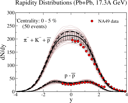
Figure 16: Rapidity distributions as indicated, with $T_{fo}=140\,$MeV. The solid lines represent the averages over the fluctuating distributions (with dispersions), whereas the dashed lines are results with the averaged initial conditions. The data are from NA49 na49 .

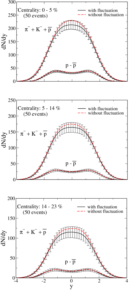
Figure 17: Centrality dependence of rapidity distributions, for Pb + Pb collisions at $\sqrt{s}=17.3\,A\,$GeV (SPS). Here, “with fluctuation” (the solid lines) means results with NeXuS fluctuating IC and “without fluctuation” (dashed lines) those with the averaged IC.

the systems, large fluctuations are expected in the initial stage of actual nuclear collisions, even for a fixed impact parameter, and that IC generated by realistic event generators do show such effects gyulassy ; nexus . Let us see in this Section what are the effects of fluctuating IC on some of the observables.

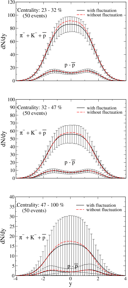
Figure 18: The same as the previous Figure, for less central events.

In gyulassy , by solving the hydrodynamic equations with longitudinal boost-invariance, it has been shown that the bumpy IC i) develop azimuthally asymmetric flows, even for central collisions, because there is no symmetry in each fluctuating event; and also ii) enhance high-$p_{T}$ direct photon yields due to the high temperature in the blobs.

Since our interest here is just to show the effects of fluctuating IC, we chose the simplest decoupling criterion, namely the usual Cooper-Frye sudden decoupling with freezeout temperature $T_{fo}$ in this Subsection.

VI.1.1 Rapidity and $m_{T}$ distributions

Let us first consider Pb + Pb collisions at SPS. In Fig. 16, we show the rapidity distributions for negative particles and $p-\bar{p}\,$, respectively, for the most central Pb + Pb collisions at $\sqrt{s}=17.3\,A\,$GeV. Each event, computed from randomly generated IC like the one shown in Figs. 1 and 2 (left), is represented by a thin curve (for each type of particle, either negatives or $p-\bar{p}$). The thick solid lines represent the averages over 50 events, with the corresponding dispersions. We compare the average distributions with the distributions computed starting from the averaged IC like the one shown in Figs. 1 and 2 (right), represented by dashed lines here. Here, we took $T_{fo}=140\,$MeV. The data points are shown for comparison na49 .

As is seen in this Figure, the rapidity distributions show large fluctuations from event to event and, although similar, there is a non-negligible difference between the average distributions and the ones obtained from the average IC, especially in the case of negative particles, constituted mostly of pions. For the same average initial energy, the multiplicity decreases about $6\sim 7\%$ if fluctuations exist, confirming what we showed in Sec. II. Finally, the data points in Fig. 16 are closer to the averaged distribution over fluctuating IC.

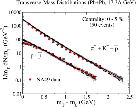
Figure 19: Transverse mass distributions as indicated, computed at $T_{fo}=140\,$MeV. The solid lines represent the averages over the fluctuating distributions (with dispersions), whereas the dashed lines are results with the averaged initial conditions. The data are from NA49 na49 .

What happens with other centralities is similar as seen in Figs. 17 and 18. Some differences are: i) as the collisions become more peripheral, naturally the dispersions increase; ii) the differences between the average distributions and the ones produced by average IC seems to decrease.

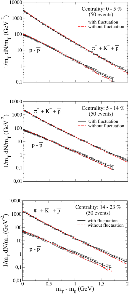
Figure 20: Centrality dependence of transverse mass distributions, for Pb + Pb collisions at $\sqrt{s}=17.3\,A\,$GeV (SPS). Here, “with fluctuation” (the solid lines) means results with NeXuS fluctuating IC and “without fluctuation” (dashed lines) those with the averaged IC.

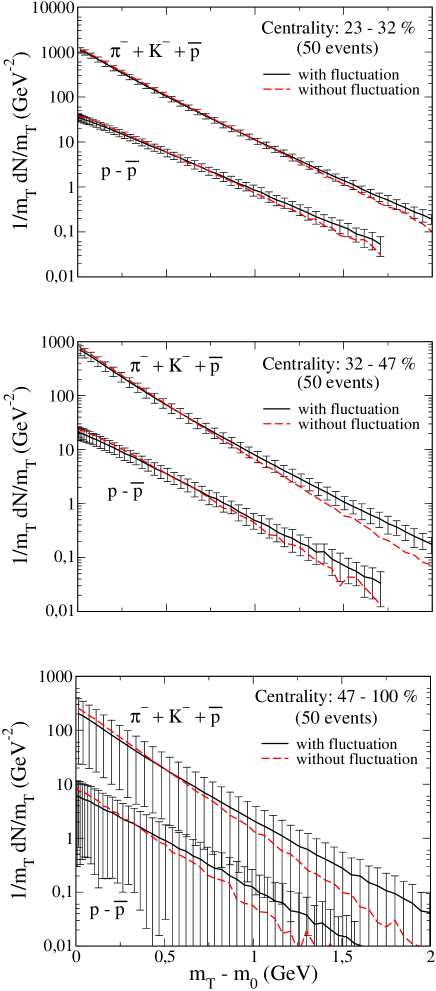
Figure 21: The same as the previous Figure, for less central events.

In Fig. 19, we show the corresponding $m_{T}$ distributions, for the most central Pb + Pb collisions at $\sqrt{s}=17.3\,A\,$GeV. One can see that apparently the fluctuation effects on the transverse-momentum spectra are very small and the averaged spectra are in good agreement with those computed with averaged IC, and also with data. This smallness of the fluctuation effects on the transverse-momentum spectra is not in contradiction with the large fluctuations we saw above of rapidity distributions. In part this is due to the logarithmic scale used here. One can conclude, however, that the IC fluctuations affect very little the slope of the $m_{T}$ spectra. This conclusion is valid for other centralities, as seen in Figs. 20 and 21, except for the most peripheral case, where the dispersions are very large. If we look more carefully, we can perceive a small difference between the averaged spectra and those computed with the averaged IC, which appears in all the centralities, that is the tail of the averaged spectra is more concave and the distributions become higher, probably because the expansion is more violent in this case, due to the high density spots in the IC.

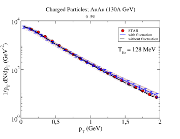
Figure 22: $p_{T}$ distributions for the most central Au+Au at 130A GeV. The data are from STAR star1 .

At RHIC energies the results are similar. In Fig. 22, we show the $p_{T}$ distributions of charged particles in the most central Au + Au collisions at 130A GeV, calculated both with NeXuS fluctuating IC and with averaged IC. Like in the case of Pb + Pb collisions at SPS, we used sudden freezeout, but with lower freezeout temperature, $T_{fo}=128\,$MeV, the same value used in eff-t to fit the inverse slope parameter of kaons, in the same collisions, as shown in Fig. 15 and Table 1 of Section V. As is seen, the fluctuation effects are small in $p_{T}$ distribution, both curves agree each other and with data, and the average over fluctuating events gives a slightly more concave shape, just like in Pb + Pb collisions at SPS.

We show in Fig. 23, the pseudorapidity distribution of charged particles in the most central Au + Au collisions at 130A GeV, calculated with NeXuS fluctuating IC and the corresponding averaged IC, and compared with data phobos . Qualitatively, the behavior is similar to the case of Pb + Pb collisions at SPS, namely the average $\eta$ distribution is close to the distribution with the averaged IC, being the latter slightly higher than the former. The difference here is smaller than at the lower energy case. Probably this is due to the decrease of $\Delta E_{i}/\!<E>$ in Eq. (9) as the incident energy increases.

Figure 23: Charged-particle pseudo-rapidity distributions for the most central Au+Au at 130A GeV. The data are from PHOBOS phobos .

VI.1.2 Elliptic-flow parameter $v_{2}$

Let us turn to the elliptic-flow parameter $v_{2}\,$, defined as the second Fourier coefficient of the azimuthal distribution voloshin

$$\frac{dN}{d\phi}\propto\left(1+2\sum_{n}v_{n}\cos\,[n(\phi-\psi)]\right)\,.$$ (121)

Thus,

$$v_{2}=<\cos\,[2(\phi-\psi)]>\,,$$ (122)

where the bracket denotes the average value and $\psi$ gives the event-dependent collision plane.

Usually, $v_{2}$ parameter is interpreted as indicating a flow asymmetry caused by the initial-condition asymmetry associated with the non-zero impact parameter. In this case, as the produced matter in the collision is likely to be flattened in the impact-parameter direction, the pressure gradient would be larger in this direction and so would be the flow. However, as mentioned at the top of this section, it was shown in Ref. gyulassy that, even for central collisions, fluctuating IC develop azimuthally asymmetric flows, because in this case there is no symmetry in each event and, experimentally, the impact parameter cannot be determined unambiguously. So, one expects larger $v_{2}$ for fluctuating IC as compared to averaged IC case. Remark that the fluctuation we are talking about is not the often discussed voloshin ; ollitrault finite-multiplicity fluctuation at the end of the process. In Fig. 24, results of NeXuS+SPheRIO for $v_{2}$ of pions produced in Pb+Pb collisions at 17.3A GeV are shown, both with fluctuating IC and averaged IC and compared with data na49 . Large discrepancy is seen between the two ways of calculating this parameter, and the data are closer to $<v_{2}>$, calculated with fluctuating IC.

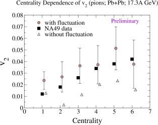
Figure 24: Centrality dependence ov $v_{2}$ for pions for Pb+Pb collisions at SPS. The data are from NA49 na49 .

VI.1.3 Two-pion interferometry

As is well known, the identical-particle correlation, also known as Hanbury-Brown-Twiss effect (HBT effect) hbt1 is a powerful tool for probing geometrical sizes of the space-time region from which they were emitted. If the source is static like a star, it is directly related to the spatial dimensions of the particle emission source. When applied to a dynamical source, however, several non-trivial effects appear hama ; pratt , reflecting its time evolution as happens in high-energy heavy-ion collisions. Being so, the inclusion of IC fluctuations may affect considerably the so-called HBT radii, because, as discussed in Sec. II, the IC in the event-by-event base often show small high-density spots in the energy distribution, and our expectation is that such spots manifest themselves at the end when particles are emitted, giving smaller HBT radii.

We shall discuss here only the recent application of NeXuS+SPheRIO code for HBT effect with IC fluctuations, for Au+Au collisions at 130A GeV fic-hbt . A more detailed account of two-particle correlations is given by Padula sandra in a separate paper in this issue.

For studying the fluctuation effects of IC on HBT correlation, first we assume Cooper-Frye sudden freezeout (FO) at $T_{f.o.}=128\,$MeV. This freezeout temperature is the same one previously found by studying the energy dependence of kaon slope parameter $T^{*}$ eff-t , discussed in Subsection V.2 and appears in Table 1. We showed in Subsection VI.1.1 that indeed this choice of $T_{f.o.}$ reproduces the $p_{T}$-distribution data at 130A GeV, both with averaged and fluctuating IC. We also neglect the resonance decays. It is argued csorgo that, since resonance decays contribute to the correlations with very small $q$ values ($q\lower 2.84544pt\hbox{$\,\buildrel<\over{\sim}\,$}q_{min}\,$, where $q_{min}$ is the minimum measureable $q$), the experimentally determined HBT radii are essentially due to the direct pions. Then the two-particle correlation function is expressed in terms of the distribution function $f(x,p)$ as

$$C_{2}(q,P)=1+\frac{|I(q,P)|^{2}}{I(0,p_{1})I(0,p_{2})}$$ (123)

where $P=(p_{1}+p_{2})/2$ and $q=(p_{1}-p_{2})$ and $p_{i}$ is the momentum of the $i$th pion. Usually

$$I(q,P)\equiv\langle a_{p_{1}}^{+}a_{p_{2}}\rangle=\int_{T_{f.o.}}d\sigma_{\mu}P^{\mu}f(x,P)e^{iqx}.$$ (124)

In SPH representation, we write $I(q,P)$ as

$$I(q,P)=\sum_{j}\frac{\nu_{j}n_{j\mu}P^{\mu}}{s_{j}|n_{j\mu}u_{j}^{\mu}|}\;{\mathrm{e}}^{iq_{\mu}x_{j}^{\mu}}f(u_{j\mu}P^{\mu})\,,$$ (125)

where the sumation is over all the SPH particles. In the Cooper-Frye freezeout, these particles should be taken where they cross the hyper-surface $T=T_{f.o.}$ and $n_{j\mu}$ is the normal to this hyper-surface. Notice that, if we put $p_{1}=p_{2}=P$, so that $q=0$, Eqs. 124 and 125 are reduced, respectively, to Eqs. 113 and 114, that is, to the inclusive one-particle distribution.

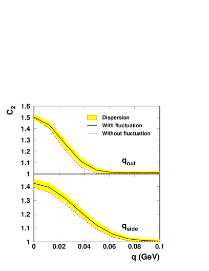
Figure 25: Correlation functions from fluctuating IC and averaged IC. Sudden freeze-out is used here. The rapidity range is $-0.5\leq Y\leq 0.5$ and $q_{o,s,l}$ which do not appear in the horizontal axis are integrated over $0\leq q_{o,s,l}\leq 35$MeV.

In Fig. 25, we compare the correlation function $C_{2}$ averaged over 15 fluctuating events with those computed starting from the averaged IC (so, without fluctuations). One can see that the IC fluctuations are reflected in large fluctuations also in the HBT correlations. When averaged, the resulting correlation $<C_{2}>$ are broader than those computed with averaged IC, so giving smaller radii as expected. Also the shape of the correlation functions changes.

We plot the $m_{T}$ dependence of HBT radii, with Gaussian fit of $C_{2}\,$, in Fig. 26, together with RHIC data star2 ; phenix and results with CE, which will be discussed in Sec. VI.2.2. It is seen that the smooth IC with sudden FO makes the $m_{T}$ dependence of $R_{o}\,$ flat or even increasing, which is in agreement with other hydro calculations morita but in conflict with the data. The fluctuating IC make the radii smaller, especially in the case of $R_{o}\,$, however without changing the $m_{T}$-dependence.

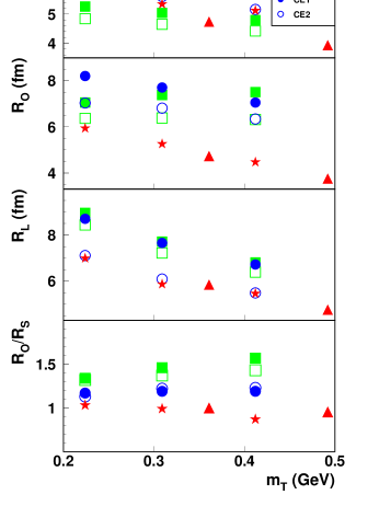
Figure 26: HBT radii and the ratio $R_{o}/R_{s}$ for sudden freeze-out (FO) and CE. 1 stands for averaged IC and 2 fluctuating IC. Data are from star2 ; phenix .

VI.2 Effects of continuous emission

As discussed in Sec. V, it is more likely that the decoupling occurs not suddenly, but continuously from any point of the fluid and at any instant of time, according to some escaping probability ${\cal P}(x,p)$ given by Eq. (117). There are several nice predictions of the Continuous Emission Model (CEM) as discussed in grassi . However, although more realistic, this description is not handy because, ${\cal P}$ depends on the momentum of the escaping particle and, moreover, on the future of the fluid as seen in Eq. (117). In order to make the computation practicable, in fic-hbt we first took ${\cal P}$ on the average, i.e.,

$${\cal P}(x,p)\Rightarrow<{\cal P}(x,p)>\equiv{\cal P}(x)\,.$$

Then, approximated linearly the density

$$\rho(x^{\prime})=\alpha s(x^{\prime})$$

(where, for example in the ideal massless pion gas case, $\alpha=(45\,\zeta(3))/2\pi^{4}=.278$) in the integral of Eq. (117). Thus,

$${\cal P}(x,p)\Rightarrow{\cal P}(x)=\exp\left(-\kappa\frac{s^{2}}{|ds/d\tau|}\right)\,,$$ (126)

where $<\sigma v>$ has been included in $\kappa=0.5\,\alpha<\sigma v>$. Although approximately, now we can compute ${\cal P}$ in each space-time point.

In Fig.27, we show the time evolution of the escaping probability ${\cal P}(x)$ given by Eq.(126) in the mid-rapidity plane for the most central Au+Au collisions at 130 A GeV. The IC have been computed at $\tau=1\,$fm and averaged over 30 NeXuS events. Here and in the computations of observables below, the parameter $\kappa$ has been estimated to be .3, corresponding to $<\sigma v>=2\,$fm² in the zero temperature limit and some 20% larger at $T=m_{\pi}\,$. As seen, the probability remains $0.1<{\cal P}(x)<0.8$ in a quite large domain, especially for $\tau>10\,$fm, indicating that both the emission zone and duration are expected to be large, in opposition to the standard sudden freezeout case. For comparison, we show also the temperature distribution in Fig.27, with some isotherms.

To calculating the spectra, now Eq. (120) is translated into SPH language, which is given by Eq. (114), but where the sum is computed in the present case not over $T=T_{f.o.}$ hypersurface but picking out SPH particles according to the probability ${\cal P}$, given by Eq. (126) with the normal $n_{j\mu}$ pointing to the 4-gradient of ${\cal P}$. Since our procedure favors emission from fast outgoing SPH “particles”, because $\rho$ decreases faster there and so does $s$ in this case making ${\cal P}$ larger, we believe that the main feature of CEM is preserved in our approximation.

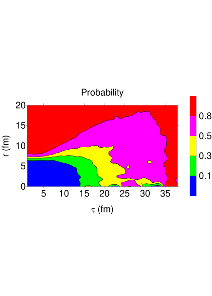
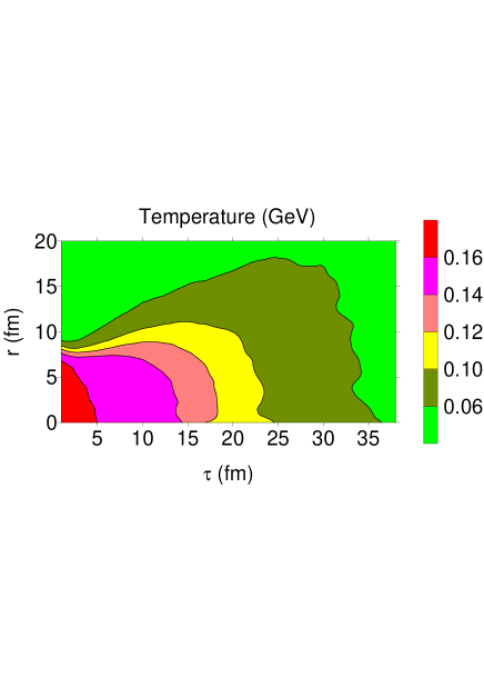
Figure 27: Upper panel: Probability distribution as given by eq.(126) for the most central Au+Au collisions at 130 A GeV, in the mid-rapidity plane for averaged IC. Lower panel: Corresponding temperature distribution.

VI.2.1 $m_{T}$ distributions

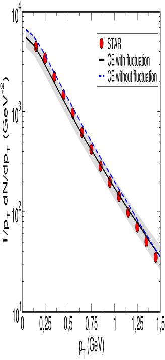
Figure 28: Charged-particle $p_{T}$ distributions in CEM for the most central Au + Au at 130A GeV. The data are from STAR star1 .

In Fig. 28, we show the charged $m_{T}$ distribution at mid-rapidity in the most central Au + Au collisions at 130A GeV, computed by using CEM, with and without fluctuations. Compare this figure with Fig. 22, where the same data are compared with calculations using sudden freezeout. One sees that, although the emission mechanisms are quite different, the results are similar, for the choice of the parameters, $T_{fo}$ in one case and $\kappa$ in the other. However, the origins of the spectrum shape are different. Whereas, in the freezeout case, all the particles are emitted at the same temperature $T_{fo}$ and the concave shape of the spectra is due to different transverse velocities of the fluid at different instants of time, in the continuous emission case, the large-$p_{T}$ particles are in general emitted earlier and at higher temperature, the small-$p_{T}$ particles are emitted later, when the fluid is cooler.

VI.2.2 Two-pion interferometry

Let us now consider the effect of continuous emission on HBT effect. Since HBT is sensitive to the space-time geometry of the fluid, and CEM produces important modification of the emission zone, we expect considerable changes in the so-called HBT radii. As mentioned above, according to this picture, the large-$p_{T}$ particles are mainly emitted at early times when the fluid is hot and mostly from its surface, whereas the small-$p_{T}$ components are emitted later when the fluid is cooler and from larger spatial domain.

In ce-hbt , we considered this effect, using the boost-invariant solution scale-invariant , and showed that whereas the so-called side radius is independent of the average $p_{T}\,$, the out radius decreases with $<p_{T}>$, because of the reason mentioned above. This behavior is expected to essentially remain in the general 3-dimensional expansion, described by SPheRIO code.

To compute the correlation function $C_{2}(q,P)$ in CEM, we first rewrite the integral (124) as

$$I(q,P) = \int_{\sigma_{0}}d\sigma_{\mu}P^{\mu}f_{free}(x_{0},P)e^{{iqx}}$$ (127)

$$+ \int d^{4}x\,\partial_{\mu}[P^{\mu}f_{free}(x,P)]e^{{iqx}},$$

which is similar to Eq. (120). Then, translate it into SPH language by using Eq. (125), but with the sum evaluated by picking out SPH particles according to the probability ${\cal P}$, given by Eq. (126) with the normal $n_{j\mu}$ pointing to the 4-gradient of ${\cal P}$, exactly in the same way as done in calculating the inclusive spectrum.

We plot in Fig. 26, some results for the $m_{T}$ dependence of HBT radii computed in this way, both with fluctuating IC and averaged IC, for Au + Au collisions at 130A GeV. For comparison, we show also the results with sudden freezeout and data star2 ; phenix . Comparing the averaged IC case (with CEM (CE1)), with the corresponding freezeout (FO1), one sees that, while $R_{L}$ remains essentially the same, $R_{s}$ decreases faster and as for $R_{o}\,$, it decreases now inverting its $m_{T}$ behavior.

In Fig. 26, one can also see the combined effect of fluctuating initial conditions together with continuous emission (curve CE2). All the radii are smaller than CE1, with averaged IC (but using CEM), as happend in the sudden freezeout case. The agreement with data is excelent both for $R_{L}$ and $R_{s}\,$, and improved considerably the results for $R_{o}$ with respect to the usual hydrodynamic description.

VII Conclusions and Outlook

In this survey, we discussed on several aspects of applications of hydrodynamic model to nucleus-nucleus collisons, giving especial emphases on i) method of solving the hydrodynamic equations for arbitrary configurations; ii) accounting for the probable event-by-event fluctuations of the initial conditions; and iii) the decoupling criteria for obtaining the observables.

The Smoothed-Particle Hydrodynamic approach, using a special hyperbolic coordinate system, is particularly interesting tool for describing rapidly expandig matter as that in high-energy nucleus-nucleus collisons, because of its efficiency and flexibility, as demonstrated through examples considered in Sec. IV.3.5, IV.3.6 and through applications, shown in Sec. VI, where the systems, in general, do not present any symmetry.

The initial conditions for hydrodynamic expansion of matter formed in relativistic heavy-ion collisions are likely neither smooth nor symmetrical, because of small size of these systems. This property has also been shown by some event generators, which take the microscopic dynamics into account. The fluctuations in the initial conditions may produce large discrepancies in the computed results for some observables, in comparison with those obtained with the usual averaged, smooth and symmetrical initial conditions. So, it is our opinion that, to extracting correct information from certain experimental data, the inclusion of the fluctuations mentioned above is mandatory.

We find that, although Cooper-Frye formula can give good results in many cases, a more realistic decoupling description is needed for obtaining many other observables. A description we proposed is the Continuous Emission Model. One typical example we showed here, in which this model improve considerably the description of data is the $m_{T}$ dependence of HBT radii, observed at RHIC.

In addition to the points summarized above, there are several basic questions to be addressed in the hydrodynamical scenary. First of all, although for the bulk properties of observables so far studied the ideal hydrodynamical description works fairly well, we still do not know how the non-equilibrium processes affect the results of these studies. This question refers both to the initial conditions and to the final particle decoupling process. For example, the present study of continuous emission showed that the real particle emission mechanism seems to be very far from the conventional Cooper-Frye scenary of sharp freeze-out surface. In Fig. 27, we showed that the escape probability ${\cal P}$ varies rather slowly both in space and time, and there is no indication of a sharp freezeout hypersurface. Another way of showing the same is given in Fig. 29, where we plotted the entropy vs. temperature of the SPH particles at the emission point. The temperature values corresponding to the particle emission spread widely. This shows that, even for a large system (Au+Au) there exists a substantial part of the system which remains out of equilibrium for a long time. Up to now, no dynamical reaction of these non-equilibrium components on the hydrodynamical evolution is studied. In this sense, it is very important to develop transport theoretical investigations yuri ; lazslo related to hydro description.

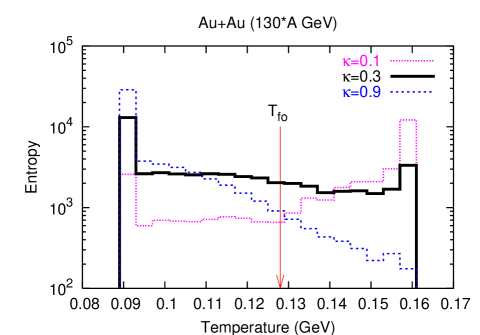
Figure 29: The entropy liberated vs. temperature of SPH particles at the decoupling point. The freeze-out temperature $T_{fo}$ used in the studies above is also shown.

Another interesting type of phenomena related to the hydrodynamical model is the ocurrence of instabilities associated to the phase transition and surface tension (finite-size effects), such as spinodal instabilities fraga04 . Some studies in this direction is in progress.

Acknowledgments

The authors are grateful to all the SPheRIO team, namely, F. Grassi. C.E. Aguiar, T. Osada, B.M. Tavares, L.L.S. Portugal, G. Grunfeld, R. Andrade, for their collaboration and stimulating discussions. Especially, the most of the hard task in the development of the code is due to T. Osada. The main part of the consideration on hadronic resonance is due to C.E. Aguiar. B.M. Tavares, L.L.S. Portugal, A.G. Grunfeld helped the construction of equations of state. We are indebted to K. Werner for valuable discussions on NeXuS event generator and for providing us with the correspondent code. Analytical solutions have been obtained in a fruitful collaboration with T. Csörgő. We are thankful to Y.M. Sinyukov and L.P. Csernai for profitable discussions on transport theoretical description of continuous emission. We also appreciated the discussions and the encouragements received from F. Pottag, S.S. Padula, F.S. Navarra, S.B. Paiva, M. Makler, M. Gorenstein, M. Gaździcki, J. Rafelski, H.T. Elze and E. Fraga.

We acknowledge financial support by FAPESP (1990/4074-5, 1993/2463-2, 1995/4635-0, 1998/2249-4, 2000/04422-7 and 2001/09861-1), CAPES/PROBRAL, CNPq, FAPERJ and PRONEX.

References

- (1) L.D. Landau, Izv. Akad. Nauk SSSR 17 (1953) 51; S.Z. Belenkij and L.D. Landau, Usp. Fiz. Nauk 56 (1955) 309; in “Collected papers of L.D. Landau” (ed. D. Ter-Haar, Pergamon, Oxford, 1965) 569 and 665.
- (2) E. Fermi, Prog. Theor. Phys. 5 (1050) 570.
- (3) P. Carruthers, Annals N.Y. Acad. Sci. 229 (1974) 91.
- (4) F. Cooper and G. Frye, Phys. Rev. D 10 (1974) 186.
- (5) T. Hirano, nucl-th/0403042.
- (6) P. Huovinen, nucl-th/0305064.
- (7) P.F. Kolb and U. Heinz, nucl-th/0305084.
- (8) K. Morita, S. Muroya, C. Nonaka and T. Hirano, Phys. Rev. C66 (2002) 054904.
- (9) S. Paiva, Y. Hama and T. Kodama, Phys. Rev. C55 (1997) 1455.
- (10) G.N. Fowler, F. Navarra, M. Plümer, A. Vourdas, R.M. Weiner and G. Wilk Phys. Rev. C40 (1989) 1219; See also F.S. Navarra, Braz. J. Phys. in this issue.
- (11) I.M. Khalatnikov, Zh. Eksp. Teor. Fiz. 27 (1954) 529; see also Landau .
- (12) M. Gyulassy, D.H. Rischke and B. Zhang, Nucl. Phys. A613 (1997) 397.
- (13) B.R. Schlei and D. Strotman, Phys. Rev. C59 (1999) 9.
- (14) C. Nonaka, E. Honda and S. Muroya, Eur. J. Phys. C17 (2000) 663.
- (15) H.J. Drescher, F.M. Liu, S. Ostrapchenko, T. Pierog and K. Werner, Phys. Rev. C65 (2002) 054902.
- (16) V.K. Magas, L.P. Csernai and D. Strottman, Phys. Rev. C64 (2001) 014901.
- (17) K.J. Eskola, P.V. Ruuskanen, S.S. Räsänen and K. Tuominen, Nucl. Phys. A696 (2001) 715.
- (18) T. Hirano and Y. Nara, nucl-th/0403029.
- (19) L.D. Landau and E.M. Lifshitz, Fluid Mechanics, second ed. Butterworth-Heinemann Ltd. Oxford (U.K.).
- (20) J. Berges, S. Borsanyi and C. Wetterich, hep-ph/0403234.
- (21) T. Kodama, H.T. Elze, C.E. Aguiar and T. Koide, cond-mat/0406732.
- (22) T. Kodama, Introduction to Relativistic Gases, in AIP Conf. Proc. 631 (2003) 3.
- (23) See for example, P. Braun-Munzinger, K. Redlich and J. Stachel, nucl-th/0304013.
- (24) E. Beth and G.E. Uhlenbeck, Physica 3 (1936) 729.
- (25) R. Dashen, S. Ma and H. Bernstein, Phys. Rev. 187 (1969) 345.
- (26) D.H. Rischke, M.I. Gorenstein, H. Stöcker and W. Greiner, Zeit. Phys. 51 (1991) 485; G.D. Yen, M.I. Gorenstein, W. Greiner and S.N. Yang, Phys.Rev. C56 (1997) 2210.
- (27) J. Sollfrank and U. Heinz, arXiv:nucl-th/9505004.
- (28) Z. Fodor and S.D. Katz, arXiv:hep-lat/0106002.
- (29) K. Rajagopal, arXiv:hep-ph/0009058.
- (30) R.C. Hwa, Phys. Rev. D10 (1974) 2260; C.B. Chiu and K.-H. Wang, Phys. Rev. D12 (1975) 272; C.B. Chiu, E.C.G. Sudarshan and K.-H. Wang, Phys. Rev. D12 (1975) 902.
- (31) J.D. Bjorken, Phys. Rev. D27 (1983) 140.
- (32) T. Csörgő, F. Grassi, Y. Hama and T. Kodama, Phys. Lett. B565 (2003) 107.
- (33) T. Csörgő, L.P. Csernai, Y. Hama and T. Kodama, Heavy Ion Phys. 21 (2004) 73; nucl-th/0306004.
- (34) H.-T. Elze, Y. Hama, T. Kodama, M. Makler and J. Rafelski, J. Phys. G25 (1999) 1935; Heavy Ion Phys. 10 (1999) 275; Proceedings of the IVth. Workshop on Quantum Chromodynamics, Paris 1998, eds. H.M. Fried and B. Müller (World Scientific, Singapura, 1999).
- (35) L.B. Lucy Astrophys. J. 82 (1977) 1013.
- (36) R.A. Gingold and J.J. Monaghan, Mon. Not. R. Astro. Soc. 181 (1977) 375.
- (37) C.E. Aguiar, T. Kodama, T. Osada and Y. Hama, J. Phys. G 27 (2001) 75; T. Kodama, C.E. Aguiar, T. Osada and Y. Hama, J. Phys. G 27 (2001) 557.
- (38) A.H. Taub, Phys. Rev. 94 (1954) 1468; J.W. Herivel, Proc. Camb. Phil. Soc. 51 (1955) 344; B.F. Schutz Jr., Phys. Rev. D2 (1970) 2762; J.R. Ray, J. Math. Phys. 13 (1972) 1451; G.Yu. Bogoslovskii, Sov. Phys. Dokl. 31 (1986) 879; T. Chiueh, Phys. Rev. E 49 (1994) 1269.
- (39) L. Mittag, M.J. Sephen and W. Yourgrau, in Variational Principles in Dynamics and Quantum Theory, ed. W.W. Yourgrau and S. Mandelstam (Dover, New York, 1968).
- (40) V.M. Strutinski, Nucl. Phys. A95 (1967) 420.
- (41) Y. Hama and F.W. Pottag, Resolution of Hydrodynamical Equations for Transverse Expansions - II, University of São Paulo print IFUSP/P-481, Aug./84.
- (42) J. Von Neumann and R.D. Richtmyer, J. Appl. Phys. 21 (1950) 232.
- (43) V. Schneider, U. Katscher, D.H. Rischke, B. Waldhauser, J.A. Maruhn and C.D. Munz, J. Comput. Phys. 105 (1993) 92.
- (44) S. Siegler and H. Riffert, astro-ph/9904070.
- (45) W. Israel, Ann. Phys. 100 (1976) 310; W. Israel and J.M. Stewart, Ann. Phys. 118 (1979) 341.
- (46) W.A. Hiscock and L. Lindbolm, Phys. Rev. D31 (1985) 725; Phys. Rev. D35 (1987) 3723.
- (47) A. Muronga, Phys. Rev. Lett. 88 (2002) 062302; A. Muronga, Phys. Rev. C69 (2004) 034903.
- (48) Y. Hama and F.S. Navarra, Z. Phys. C53 (1992) 501.
- (49) British-Scandinavian Collab., B. Alper et al., Nucl. Phys. B100 (1975) 237; F.W. Büsser et al., Phys. Lett. 46B (1973) 471 and Nucl. Phys. B106 (1976) 1; K. Eggert et al., Nucl. Phys. B98 (1975) 49; British-Scandinavian-MIT Collab., K. Guettler et al., Phys. Lett. 64B (1976) 111; Nucl. Phys. B116 (1976) 77.
- (50) UA1 Collab., C. Albajar et al., Nucl. Phys. B335 (1990) 261; UA2 Collab., M. Banner et al. Phys. Lett. 115B (1982) 59; Phys. Lett. 122B (1983) 322; Z. Phys. C27 (1985) 329; UA5 Collab., G.J. Alner et al., Nucl. Phys. B258 (1985) 505; UA5 Collab., R.E. Ansorge et al., Phys. Lett. 199B (1987) 311.
- (51) T. Alexopoulos et al., Phys. Rev. Lett. 64 (1990) 991.
- (52) F.S. Navarra, M.C. Nemes, U. Ornik and S.M. Paiva, Phys. Rev. C45 (1992) R2552.
- (53) Nu Xu and M. Kaneta, Nucl. Phys. A698 (2002) 306.
- (54) M. Gaździcki, M.I. Gorenstein, F. Grassi, Y. Hama, T. Kodama and O. Socolowski Jr., Braz. J. Phys. 34 (2004) 322-325; Y. Hama, F. Grassi, O. Socolowski Jr., T. Kodama, M. Gaździcki and M.I. Gorenstein, Acta Phys. Polon. B35 (2004) 179-182.
- (55) M.I. Gorenstein, M. Gaździcki and K.A. Bugaev, Phys. Lett. B567 (2003) 175.
- (56) E866 Collab., L. Ahle et al., Phys. Lett. B490 (2000) 53; NA49 Collab., S.V. Afanasiev et al., Phys. Rev. C66 (2002) 054902; BRAHMS Collab., D. Ouerdane et al., Nucl. Phys. A715 (2003) 478; STAR Collab., C. Adler et al., nucl-ex/0206008.
- (57) F. Grassi, Y. Hama and T. Kodama, Phys. Lett. B355 (1996) 9; F. Grassi, Y. Hama and T. Kodama, Z. Phys. C73 (1996) 153.
- (58) F. Grassi, Braz. J. Phys. in this issue.
- (59) T. Osada, C.E. Aguiar, Y. Hama and T. Kodama, nucl-th/0102011; C.E. Aguiar, Y. Hama, T. Kodama and T. Osada, Nucl. Phys. A698 (2002) 639;
- (60) C.E. Aguiar, Y. Hama, T. Kodama and T. Osada, in AIP Conf. Proc. 631 (2003) 686-694; “Event-by-event fluctuation of the initial conditions in hydrodynamic model”, Y. Hama, F. Grassi, O. Socolowski Jr., C.E. Aguiar, T. Kodama, L.L.S. Portugal, B.M. Tavares and T. Osada, in Proc. of 32 ISMD, eds. A. Sissakian, G. Kozlov and E. Kolganova, (World Scientific - Singapore, 2003), 65-68.
- (61) O. Socolowski Jr., F. Grassi, Y. Hama and T. Kodama, hep-ph/0405181.
- (62) H. Appelshäuser et al., NA49 Collab., Phys. Rev. Lett. 82 (1999) 2471; A.M. Poskanzer, nucl-ex/0110013.
- (63) PHOBOS Collaboration, B.B. Back et al., Phys. Rev. Lett. 87 (2001) 102303.
- (64) STAR Collab. C. Adler et al., Phys. Rev. Lett. 87 (2001) 112303.
- (65) S. Voloshin and Y. Zhang, Z. Phys. C70 (1996) 665.
- (66) J.-Y. Ollitrault, nucl-ex/9711003.
- (67) R. Hanbury-Brown and R.Q. Twiss, Phil. Mag. Ser. 7, Vol. 45 (1954) 663.
- (68) Y. Hama and Sandra S. Padula, Phys. Rev. D37 (1988) 3237.
- (69) S. Pratt, Phys. Rev. D33 (1986) 1314; K. Kolehmainen and M. Gyulassy, Phys. Lett. B180 (1986) 203; A.N. Makhlin and Yu.M. Sinyukov, Z. Phys. C39 (1988) 69.
- (70) Sandra S. Padula, Braz. J. Phys. in this issue.
- (71) S. Nickerson, T Csörgő and D. Kiang, Phys. Rev. C57, 3251 (1998).
- (72) STAR Collab., C. Adler et al., Phys. Rev. Lett. 87 (2001) 082301.
- (73) PHENIX Collab., K. Adcox et al., Phys. Rev. Lett. 88, 192302 (2002).
- (74) F. Grassi, Y. Hama, S.S. Padula and O. Socolowski Jr., Phys. Rev. C62 (2000) 044904.
- (75) Yu. M. Sinyukov, S. V. Akkelin and Y. Hama, Phys. Rev. Lett. 89, 052301 (2002).
- (76) C. Anderlik et al. Phys. Rev. C59, 3309 (1999); V. K. Magas et al., Acta Phys. Hung. New Ser.Heavy Ion Phys. 9, 193 (1999); V. K. Magas et al., Phys. Lett. B459, 33 (1999).
- (77) C.E. Aguiar, E.S. Fraga and T. Kodama, Braz. J. Phys. 34, 307 (2004).